Abstract

We present a phenomenological study of $\tau$-sleptons $\tilde{\tau}_{1,2}$ and $\tau$-sneutrinos $\tilde{\nu}_{\tau}$ in the Minimal Supersymmetric Standard Model with complex parameters $A_{\tau}$, $\mu$ and $M_{1}$. We analyse production and decays of the $\tilde{\tau}_{1,2}$ and $\tilde{\nu}_{\tau}$ at a future $e^{+}e^{-}$ collider. We present numerical predictions for the important decay rates, paying particular attention to their dependence on the complex parameters. The branching ratios of the fermionic decays of $\tilde{\tau}_{1}$ and $\tilde{\nu}_{\tau}$ show a significant phase dependence for $\tan\beta\raise 1.29167pt\hbox{$<$\kern-7.5pt\lower 4.30554pt\hbox{$\sim$}}10$. For $\tan\beta\raise 1.29167pt\hbox{$>$\kern-7.5pt\lower 4.30554pt\hbox{$\sim$}}10$ the branching ratios for the $\tilde{\tau}_{2}$ decays into Higgs bosons depend very sensitively on the phases. We show how information on the phase $\varphi_{A_{\tau}}$ and the other fundamental $\tilde{\tau}_{i}$ parameters can be obtained from measurements of the $\tilde{\tau}_{i}$ masses, polarized cross sections and bosonic and fermionic decay branching ratios, for small and large $\tan\beta$ values. We estimate the expected errors of these parameters. Given favorable conditions, the error of $A_{\tau}$ is about 10% to 20%, while the errors of the remaining stau parameters are in the range of approximately 1% to 3%. We also show that the induced electric dipole moment of the $\tau$–lepton is well below the current experimental limit.

1 Introduction

So far most phenomenological studies on supersymmetric (SUSY) particle searches have been performed within the Minimal Supersymmetric Standard Model (MSSM) with real SUSY parameters. In this paper we study the production and decays of $\tau$-sleptons and $\tau$-sneutrinos at an $e^{+}e^{-}$ linear collider in the MSSM with complex SUSY parameters.

In the SUSY extension of the Standard Model (SM) one introduces scalar leptons $\tilde{\ell}_{L}$, $\tilde{\ell}_{R}$, scalar neutrinos $\tilde{\nu}_{\ell}$ and scalar quarks $\tilde{q}_{L}$, $\tilde{q}_{R}$ as the SUSY partners of the leptons $\ell_{L,R}$, neutrinos $\nu_{\ell}$ and quarks $q_{L,R}$, respectively [1]. For each definite fermion flavor the states $\tilde{f}_{L}$ and $\tilde{f}_{R}$ are mixed by Yukawa terms. The mass eigenstates are $\tilde{f}_{1}$ and $\tilde{f}_{2}$, with $m_{\tilde{f}_{1}}<m_{\tilde{f}_{2}}$ [2]. For the sfermions of the first and second generation $\tilde{f}_{L}-\tilde{f}_{R}$ mixing can be neglected. For the third generation sfermions, however, $\tilde{f}_{L}-\tilde{f}_{R}$ mixing has to be taken into account due to the larger Yukawa coupling [3, 4].

In the case of the $\tau$-sleptons $\tilde{\tau}_{L}-\tilde{\tau}_{R}$ mixing is important if the SUSY parameter $\tan\beta$ is large, $\tan\beta\;\raisebox{-3.87495pt}{$\textstyle\stackrel{{\scriptstyle\textstyle>}}{{\sim}}$}\;20$. The lower mass eigenvalue $m_{\tilde{\tau}_{1}}$ can be rather small and the $\tilde{\tau}_{1}$ could be the lightest charged SUSY particle. The experimental search for the $\tau$-sleptons and the $\tau$-sneutrino and the determination of their parameters is, therefore, an important issue at all present and future colliders. Pair production of $\tau$-sleptons and $\tau$-sneutrinos will be particularly interesting at an $e^{+}e^{-}$ linear collider with centre of mass energy $\sqrt{s}=0.5-1.2$ TeV. At such a collider and with an integrated luminosity of about $500$ fb^-1 it will be possible to measure masses, cross sections and decay branching ratios with high precision [5, 6]. This will allow us to obtain information on the fundamental soft SUSY breaking parameters of the third generation slepton system.

In the recent phenomenological study of 3rd generation sfermions in the real MSSM it has been shown how the masses and the mixing angle of the stop system can be determined by measurements of the production cross sections with polarized beams [7]. The results of a simulation of $e^{+}e^{-}\to\tilde{t}_{1}\bar{\tilde{t}_{1}}$ with the decay modes $\tilde{t}_{1}\to\tilde{\chi}^{0}_{1}c$ and $\tilde{t}_{1}\to\tilde{\chi}^{+}_{1}b$ and including full SM background in [8] imply that with an integrated luminosity of $500$ fb^-1 an accuracy of the order of $1\%$ or better may be obtained. The numerical precision to be expected for the determination of the underlying SUSY parameters $M_{\tilde{Q}}$, $M_{\tilde{U}}$ and (real) $A_{t}$ has also been given. For low $\tan\beta$ one can expect similar results for the sbottom and stau systems [5, 6, 7].

The assumption of real SUSY parameters has partly been justified by the very small experimental upper limits on the electric dipole moments (EDM) of electron and neutron. A possibility to avoid the EDM constraints is to assume that the masses of the first and second generation sfermions are large (above the TeV scale), while the masses of the third generation sfermions are small (below $1$ TeV) [9]. Another possibility is suggested by recent analyses of the EDMs, which have shown that strong cancellations between the different SUSY contributions to the EDMs can occur [10]. As a consequence of these cancellations it has turned out that the complex phase of the Higgs–higgsino mass parameter $\mu$ is much less restricted than previously assumed, whereas the complex phases of the soft–breaking trilinear scalar coupling parameters $A_{f}$ are practically unconstrained [11, 12]. For example, in a mSUGRA–type model with universal parameters $M_{1/2}$, $M_{0}$, $\tan\beta$ and complex $A_{0}$, with $|\mu|^{2}$ being determined by radiative electroweak symmetry breaking, the phase of $\mu$ is constrained to $|\varphi_{\mu}|\raise 1.29167pt\hbox{$<$\kern-7.5pt\lower 4.30554pt\hbox{$\sim$}}0.1-0.2$ for low values of the scalar mass parameter, $M_{0}\raise 1.29167pt\hbox{$<$\kern-7.5pt\lower 4.30554pt\hbox{$\sim$}}400$ GeV, and becomes less constrained for higher values of $M_{0}$. The phase of $A_{0}$, $\varphi_{A_{0}}$, turns out to be correlated with $\varphi_{\mu}$, but otherwise not restricted [12, 13]. In models with more general parameter specifications also $\varphi_{\mu}$ turns out to be less constrained [14]. In any case, this means that in a complete phenomenological analysis of production and decays of third generation sfermions one has to take into account that the SUSY parameters $\mu$ and $A_{f}$ may be complex and one has to study the implications that follow for the important observables.

In our present phenomenological study of 3rd generation sleptons we use the MSSM as general framework and we assume that the parameters $\mu$, $A_{\tau}$ and $M_{1}$ are complex ($A_{\tau}$ is the trilinear scalar coupling parameter of the $\tilde{\tau}_{i}$-system and $M_{1}$ is the $U(1)$ gaugino mass parameter). We neglect flavor changing $CP$ violating phases and assume that the scalar mass matrices and trilinear scalar coupling parameters are flavor diagonal. We perform an analysis of production and decay rates of $\tilde{\tau}_{1}$, $\tilde{\tau}_{2}$ and $\tilde{\nu}_{\tau}$ at an $e^{+}e^{-}$ linear collider with a CMS energy $\sqrt{s}=0.5-1.2$ TeV. We include also explicit $CP$ violation in the Higgs sector induced by stop and sbottom loops with complex parameters as in [15, 16] and [17], using the loop–corrected formulae of [15]. Our present study is an extension of the corresponding one in the MSSM with real parameters in [7]. Compared to the real MSSM, the inclusion of the complex phases $\varphi_{A_{\tau}}$, $\varphi_{\mu}$ and $\varphi_{U(1)}$ of $A_{\tau}$, $\mu$ and $M_{1}$ means that the number of independent fundamental SUSY parameters is increased. In order to determine all these parameters one has to measure more independent observables than in the real case.

In principle, the imaginary parts of the complex parameters involved could most directly and unambiguously be determined by measuring suitable $CP$ violating observables. However, in the $\tilde{\tau}_{i}$-system this is not straightforward, because the $\tilde{\tau}_{i}$ are spinless and their main decay modes are two–body decays. A possible method has been proposed in [18], which is applicable if the mass splitting between the mass eigenstates $\tilde{\tau}_{1}$ and $\tilde{\tau}_{2}$ is very small. If $m_{\tilde{\tau}_{1}}-m_{\tilde{\tau}_{2}}$ is of the order of the decay widths, $\tilde{\tau}_{1}-\tilde{\tau}_{2}$ oscillations will occur which can lead to large $CP$ violating asymmetries in $e^{+}e^{-}$ annihilation. In Ref. [19] an analysis of $\mu^{+}\mu^{-}\rightarrow\tilde{\tau}_{i}\bar{\tilde{\tau}_{j}}$ with longitudinally and transversely polarized beams has been given and the observables sensitive to $CP$ violation in the $\tilde{\tau}_{i}$ sector and Higgs sector have been classified.

On the other hand, also the $CP$ conserving observables depend on the phases of the underlying complex parameters, because the mass eigenvalues and the couplings involved are functions of these parameters. In particular, the various decay branching ratios depend in a characteristic way on the complex phases. The main purpose of the present paper is a detailed study of the fermionic decay branching ratios of $\tilde{\tau}_{1}$, $\tilde{\tau}_{2}$ and $\tilde{\nu}_{\tau}$, and the bosonic decay branching ratios of $\tilde{\tau}_{2}$ and $\tilde{\nu}_{\tau}$ and their dependences on the phases $\varphi_{A_{\tau}}$, $\varphi_{\mu}$ and $\varphi_{U(1)}$. In [20] we have published first results of our study. In the present paper we give the analytic expressions for the various decay widths with complex couplings. We present a more detailed numerical study of the phase dependences of the various branching ratios. We also discuss how these phase dependences can be qualitatively understood on the basis of the analytic expressions for the decay widths. Furthermore, we give a theoretical estimate of the precision to be expected for the determination of the complex phases together with the other fundamental parameters of the $\tilde{\tau}_{i}$-system by measurements of suitable decay branching ratios as well as masses and polarized production cross sections in $e^{+}e^{-}$ annihilation. Finally, we calculate the EDM of the $\tau$-lepton induced by the $\tau$-slepton–neutralino and $\tau$-sneutrino–chargino loops with complex $A_{\tau}$, $\mu$ and $M_{1}$.

In Section 2 we shortly review the mixing of 3rd generation sleptons in the presence of complex parameters. In Section 3 we give the formulae for the fermionic and bosonic decay widths of $\tilde{\tau}_{i}$ and $\tilde{\nu}_{\tau}$. In Section 4 we present numerical results for the phase dependences of their branching ratios. In Section 5 we give an estimate of the errors to be expected for the fundamental parameters and the phases of $A_{\tau}$, $\mu$ and $M_{1}$. In Section 6 we present our results for the EDM of the $\tau$. Section 7 contains a short summary.

2 $\tilde{\tau}_{L}-\tilde{\tau}_{R}$ Mixing

We first give a short account of $\tilde{\tau}_{L}-\tilde{\tau}_{R}$ mixing in the case the parameters $\mu$ and $A_{\tau}$ are complex. The masses and couplings of the $\tau$-sleptons follow from the hermitian $2\times 2$ mass matrix which in the basis $(\tilde{\tau}_{L},\tilde{\tau}_{R})$ reads [2, 21]

$${\mathcal{L}}_{M}^{\tilde{\tau}}=-(\tilde{\tau}_{L}^{\ast},\,\tilde{\tau}_{R}^{\ast})\left(\begin{array}[]{ccc}M_{\tilde{\tau}_{LL}}^{2}&e^{-i\varphi_{\tilde{\tau}}}|M_{\tilde{\tau}_{LR}}^{2}|\\[14.22636pt] e^{i\varphi_{\tilde{\tau}}}|M_{\tilde{\tau}_{LR}}^{2}|&M_{\tilde{\tau}_{RR}}^{2}\end{array}\right)\left(\begin{array}[]{ccc}\tilde{\tau}_{L}\\[14.22636pt] \tilde{\tau}_{R}\end{array}\right),$$ (1)

with

$$M_{\tilde{\tau}_{LL}}^{2} = M_{\tilde{L}}^{2}+(-\frac{1}{2}+\sin^{2}\Theta_{W})\cos 2\beta\ m_{Z}^{2}+m_{\tau}^{2},$$ (2)

$$M_{\tilde{\tau}_{RR}}^{2} = M_{\tilde{E}}^{2}-\sin^{2}\Theta_{W}\cos 2\beta\ m_{Z}^{2}+m_{\tau}^{2},$$ (3)

$$M_{\tilde{\tau}_{RL}}^{2} = (M_{\tilde{\tau}_{LR}}^{2})^{\ast}=m_{\tau}(A_{\tau}-\mu^{\ast}\tan\beta),$$ (4)

$$\varphi_{\tilde{\tau}}=\arg[A_{\tau}-\mu^{\ast}\tan\beta],$$ (5)

where $m_{\tau}$ is the mass of the $\tau$-lepton, $\Theta_{W}$ is the weak mixing angle, $\tan\beta=v_{2}/v_{1}$ with $v_{1}(v_{2})$ being the vacuum expectation value of the Higgs field $H_{1}^{0}(H_{2}^{0})$, and $M_{\tilde{L}}$, $M_{\tilde{E}},A_{\tau}$ are the soft SUSY–breaking parameters of the $\tilde{\tau}_{i}$ system. The $\tilde{\tau}$ mass eigenstates are $(\tilde{\tau}_{1},\tilde{\tau}_{2})=(\tilde{\tau}_{L},\tilde{\tau}_{R}){\mathcal{R}^{\tilde{\tau}}}^{T}$ with

$$\mathcal{R}^{\tilde{\tau}}=\left(\begin{array}[]{ccc}e^{i\varphi_{\tilde{\tau}}}\cos\theta_{\tilde{\tau}}&\sin\theta_{\tilde{\tau}}\\[14.22636pt] -\sin\theta_{\tilde{\tau}}&e^{-i\varphi_{\tilde{\tau}}}\cos\theta_{\tilde{\tau}}\end{array}\right),$$ (6)

and

$$\cos\theta_{\tilde{\tau}}=\frac{-|M_{\tilde{\tau}_{LR}}^{2}|}{\sqrt{|M_{\tilde{\tau}_{LR}}^{2}|^{2}+(m_{\tilde{\tau}_{1}}^{2}-M_{\tilde{\tau}_{LL}}^{2})^{2}}},\quad\sin\theta_{\tilde{\tau}}=\frac{M_{\tilde{\tau}_{LL}}^{2}-m_{\tilde{\tau}_{1}}^{2}}{\sqrt{|M_{\tilde{\tau}_{LR}}^{2}|^{2}+(m_{\tilde{\tau}_{1}}^{2}-M_{\tilde{\tau}_{LL}}^{2})^{2}}}.$$ (7)

The mass eigenvalues are

$$m_{\tilde{\tau}_{1,2}}^{2}=\frac{1}{2}\left((M_{\tilde{\tau}_{LL}}^{2}+M_{\tilde{\tau}_{RR}}^{2})\mp\sqrt{(M_{\tilde{\tau}_{LL}}^{2}-M_{\tilde{\tau}_{RR}}^{2})^{2}+4|M_{\tilde{\tau}_{LR}}^{2}|^{2}}\right).$$ (8)

The ${\tilde{\nu}}_{\tau}$ appears only in the left–state. Its mass is given by

$$m^{2}_{\tilde{\nu}_{\tau}}=M^{2}_{\tilde{L}}+\frac{1}{2}m^{2}_{Z}\cos 2\beta\,.$$ (9)

Eqs. (7) and (8) show that the phase dependence of the mixing angle $\theta_{\tilde{\tau}}$ and the eigenvalues $m_{\tilde{\tau}_{1,2}}$ stems from the term $m^{2}_{\tau}|A_{\tau}||\mu|\tan\beta\cos(\varphi_{\mu}+\varphi_{A_{\tau}})$. The phase dependence of $\theta_{\tilde{\tau}}$ is strongest if $|A_{\tau}|\approx|\mu|\tan\beta$ and at the same time $|M_{\tilde{\tau}_{LL}}^{2}-M_{\tilde{\tau}_{RR}}^{2}|\;\raisebox{-3.87495pt}{$\textstyle\stackrel{{\scriptstyle\textstyle<}}{{\sim}}$}\;|M_{\tilde{\tau}_{LR}}^{2}|$. The masses $m_{\tilde{\tau}_{1,2}}$ are in many cases insensitive to the phases $\varphi_{\mu}$ and $\varphi_{A_{\tau}}$ because $m_{\tau}$ is small.

3 Production and Decay Formulae of $\tilde{\tau}_{i}$ and $\tilde{\nu}_{\tau}$

The reaction $e^{+}e^{-}\rightarrow\tilde{\tau}_{i}\bar{\tilde{\tau}_{j}}$ proceeds via $\gamma$ and $Z$ exchange in the $s$-channel. The $Z\tilde{\tau}_{i}\tilde{\tau}_{j}$ couplings are

$$C(\tilde{\tau}_{1}^{\ast}Z\tilde{\tau}_{1}) = \frac{1}{2\cos\Theta_{W}}(\cos^{2}\theta_{\tilde{\tau}}-2\sin^{2}\Theta_{W}),$$

$$C(\tilde{\tau}_{2}^{\ast}Z\tilde{\tau}_{2}) = \frac{1}{2\cos\Theta_{W}}(\sin^{2}\theta_{\tilde{\tau}}-2\sin^{2}\Theta_{W}),$$

$$C(\tilde{\tau}_{2}^{\ast}Z\tilde{\tau}_{1}) = -\frac{1}{2\cos\Theta_{W}}e^{-i\varphi_{\tilde{\tau}}}\cos\theta_{\tilde{\tau}}\sin\theta_{\tilde{\tau}}$$

$$C(\tilde{\tau}_{1}^{\ast}Z\tilde{\tau}_{2}) = [C(\tilde{\tau}_{2}^{*}Z\tilde{\tau}_{1})]^{\ast}.$$ (10)

The reaction $e^{+}e^{-}\to\tilde{\nu}_{\tau}\bar{\tilde{\nu}_{\tau}}$ proceeds via $s$-channel $Z$ exchange with the coupling

$$C(\tilde{\nu}_{\tau}^{\ast}Z\tilde{\nu}_{\tau})=-\frac{1}{2\cos\Theta_{W}}\,.$$ (11)

The cross section of $e^{+}e^{-}\to\tilde{\nu}_{\tau}\bar{\tilde{\nu}_{\tau}}$ at tree level does not depend on the phases $\varphi_{\mu}$ and $\varphi_{A_{\tau}}$. The tree–level cross sections of the reactions $e^{+}e^{-}\rightarrow\tilde{\tau}_{i}\bar{\tilde{\tau}_{j}}$ do not explicitly depend on the phases $\varphi_{\mu}$ and $\varphi_{A_{\tau}}$, because the couplings $C(\tilde{\tau}_{i}^{\ast}Z\tilde{\tau}_{i}),i=1,2$, are real and in $e^{+}e^{-}\rightarrow\tilde{\tau}_{1}\bar{\tilde{\tau}_{2}}$ only $Z$ exchange contributes. The cross sections depend only on the mass eigenvalues $m_{\tilde{\tau}_{1,2}}$ and on the mixing angle $\theta_{\tilde{\tau}}$. Therefore, they depend only implicitly on the phases via the $\cos(\varphi_{\mu}+\varphi_{A_{\tau}})$ dependence of $m_{\tilde{\tau}_{1,2}}$ and $\theta_{\tilde{\tau}}$, Eqs. (7) and (8). This holds even if one or both beams are polarized (the formulae of the cross sections including beam polarizations are given, e. g., in [22]). Of course, properly polarized $e^{-}$ and $e^{+}$ beams are a very useful tool to enhance some signals and reduce the background and, therefore, measure some of the observables with better precision [7, 23]. Information about the phases $\varphi_{\mu}$ and $\varphi_{A_{\tau}}$ separately can be obtained by studying the branching ratios of the $\tilde{\tau}_{i}$ and $\tilde{\nu}_{\tau}$ decays into neutralinos, charginos and Higgs bosons, because some of them depend explicitly on the phases. It is expected that Yukawa–type corrections at one–loop order to the $\tilde{\tau}_{i}$ and $\tilde{\nu}_{\tau}$ pair production cross sections and decay widths will not change the overall picture obtained in tree approximation, because they have been shown to be of the order of a few percent only [24].

3.1 Fermionic Decay Widths of $\tilde{\tau}_{i}$ and $\tilde{\nu}_{\tau}$

The widths for the decays $\tilde{\tau}_{i}\rightarrow\tilde{\chi}_{j}^{0}\tau(\lambda_{\tau}),i=1,2,j=1,\dots,4$, where $\tilde{\chi}_{j}^{0}$ is the neutralino and $\lambda_{\tau}=\pm\frac{1}{2}$ is the helicity of the outgoing $\tau$, read

$$\Gamma(\tilde{\tau}_{i}\rightarrow\tilde{\chi}_{j}^{0}\tau(\lambda_{\tau}))=\frac{g^{2}\kappa(m_{\tilde{\tau}_{i}}^{2},m_{\tilde{\chi}_{j}^{0}}^{2},m_{\tau}^{2})}{16\pi m_{\tilde{\tau}_{i}}^{3}}\ |\mathcal{M}_{\lambda_{\tau}}|^{2}\quad$$ (12)

with

$$|\mathcal{M}_{\lambda_{\tau}}|^{2} = \frac{1}{4}\biggl{(}H_{s}^{2}\Bigl{(}|b_{ij}^{\tilde{\tau}}|^{2}+|a_{ij}^{\tilde{\tau}}|^{2}+2\Re e({b_{ij}^{\tilde{\tau}}}^{\ast}a_{ij}^{\tilde{\tau}})\Bigr{)}+{}$$ (13)

$${}+H_{p}^{2}\Bigl{(}|b_{ij}^{\tilde{\tau}}|^{2}+|a_{ij}^{\tilde{\tau}}|^{2}-2\Re e({b_{ij}^{\tilde{\tau}}}^{\ast}a_{ij}^{\tilde{\tau}})\Bigr{)}+{}$$

$${}+2\,(-1)^{\lambda_{\tau}+\frac{1}{2}}\,H_{p}H_{s}\Bigl{(}|a_{ij}^{\tilde{\tau}}|^{2}-|b_{ij}^{\tilde{\tau}}|^{2}\Bigr{)}\Biggr{)}\quad$$

where $g$ is the weak $SU(2)$ gauge coupling constant, $\kappa(x,y,z)=(x^{2}+y^{2}+z^{2}-2xy-2xz-2yz)^{1/2}$ and $H_{s}=(m_{\tilde{\tau}_{i}}^{2}-(m_{\tilde{\chi}_{j}^{0}}+m_{\tau})^{2})^{\frac{1}{2}},H_{p}=(m_{\tilde{\tau}_{i}}^{2}-(m_{\tilde{\chi}_{j}^{0}}-m_{\tau})^{2})^{\frac{1}{2}}$. The couplings are

$$a_{ij}^{\tilde{\tau}}=(\mathcal{R}^{\tilde{\tau}}_{in})^{\ast}\mathcal{A}^{\tau}_{jn},\qquad b_{ij}^{\tilde{\tau}}=(\mathcal{R}^{\tilde{\tau}}_{in})^{\ast}\mathcal{B}^{\tau}_{jn},\qquad\ell_{ij}^{\tilde{\tau}}=(\mathcal{R}^{\tilde{\tau}}_{in})^{\ast}\mathcal{O}^{\tau}_{jn}\qquad(n=L,R)$$ (14)

where

$$\mathcal{A}^{\tau}_{j}=\left(\begin{array}[]{ccc}f^{\tau}_{Lj}\\[5.69054pt] h^{\tau}_{Rj}\end{array}\right),\qquad\mathcal{B}^{\tau}_{j}=\left(\begin{array}[]{ccc}h^{\tau}_{Lj}\\[5.69054pt] f^{\tau}_{Rj}\end{array}\right),\qquad\mathcal{O}^{\tau}_{j}=\left(\begin{array}[]{ccc}-U_{j1}\\[5.69054pt] Y_{\tau}U_{j2}\end{array}\right)$$ (15)

with

$$h^{\tau}_{Lj} = (h^{\tau}_{Rj})^{\ast}=Y_{\tau}N_{j3}^{\ast}$$

$$f^{\tau}_{Lj} = -\frac{1}{\sqrt{2}}(\tan\Theta_{W}N_{j1}+N_{j2})$$

$$f^{\tau}_{Rj} = \sqrt{2}\tan\Theta_{W}N_{j1}^{\ast}.$$ (16)

$Y_{\tau}=m_{\tau}/(\sqrt{2}m_{W}\cos\beta)$ is the $\tau$ Yukawa coupling. The mixing matrices $U$ and $N$ are defined by Eqs. (40) and (50) in Appendices A and B. Since $m_{\tau}\ll m_{\tilde{\tau}_{1}}$, we have $H_{s}\approx H_{p}$ and, hence, to a good approximation, $\Gamma(\tilde{\tau}_{i}\to\tilde{\chi}_{j}^{0}\tau(\lambda_{\tau}))\propto|b_{ij}^{\tilde{\tau}}|^{2}(|a_{ij}^{\tilde{\tau}}|^{2})$ for $\lambda_{\tau}=+\frac{1}{2}(-\frac{1}{2})$ [25].

The width for the decay into the chargino, $\tilde{\tau}_{i}\rightarrow\tilde{\chi}_{j}^{-}\nu_{\tau}(i,j=1,2)$, is obtained by the replacements $a_{ij}^{\tilde{\tau}}\to\ell_{ij}^{\tilde{\tau}},b_{ij}^{\tilde{\tau}}\to 0,m_{{\tilde{\chi}}_{j}^{0}}\to m_{{\tilde{\chi}}_{j}^{-}},m_{\tau}\to 0$ and $\lambda_{\tau}\to-\frac{1}{2}$ in Eqs. (12) and (13), with the couplings $\ell_{ij}^{\tilde{\tau}}$ also given in Eqs. (14) and (15). The width for the $\tau$-sneutrino decay $\tilde{\nu}_{\tau}\rightarrow\tilde{\chi}_{j}^{0}\nu_{\tau}$ is obtained by the replacements $a_{ij}^{\tilde{\tau}}\to a_{j}^{\tilde{\nu}}$, $b_{ij}^{\tilde{\tau}}\to 0$, $m_{{\tilde{\tau}}_{i}}\to m_{{\tilde{\nu}}_{\tau}}$, $m_{\tau}\to 0$ and $\lambda_{\tau}\to-\frac{1}{2}$ in Eqs. (12) and (13), and that for the decay $\tilde{\nu}_{\tau}\rightarrow\tilde{\chi}_{j}^{+}\tau(\lambda_{\tau})$ by the replacements $a_{ij}^{\tilde{\tau}}\to\ell_{j}^{\tilde{\nu}},b_{ij}^{\tilde{\tau}}\to k_{j}^{\tilde{\nu}}$, $m_{{\tilde{\tau}}_{i}}\to m_{{\tilde{\nu}}_{\tau}}$ and $m_{{\tilde{\chi}}^{0}_{j}}\to m_{{\tilde{\chi}}^{+}_{j}}$. The couplings are now

$$a^{\tilde{\nu}}_{j}=\frac{1}{\sqrt{2}}(N_{j1}\tan\Theta_{W}-N_{j2}),\qquad k^{\tilde{\nu}}_{j}=Y_{\tau}U_{j2}^{\ast},\qquad\ell^{\tilde{\nu}}_{j}=-V_{j1}\,,$$ (17)

with the mixing matrix $V$ given by Eq. (41) in Appendix A.

As can be seen, the widths for the decays of $\tilde{\tau}_{1}$ and $\tilde{\tau}_{2}$ into charginos and neutralinos depend on $\cos(\varphi_{\mu}+\varphi_{A_{\tau}})$ through $m_{\tilde{\tau}_{i}}$ and $\theta_{\tilde{\tau}}$, and also on $\varphi_{\tilde{\tau}}$, Eq. (5). They depend also on $\varphi_{\mu}$ ($\varphi_{\mu}$ and $\varphi_{U(1)}$) via the chargino (neutralino) masses $m_{\tilde{\chi}_{j}^{-}}(m_{\tilde{\chi}_{j}^{0}})$ and mixing matrix $U(N)$, see Eqs. (39-48) (Eqs. (49,50)). The widths for the $\tilde{\nu}_{\tau}$ decays into fermions depend on the phases of $\varphi_{\mu}$ and $\varphi_{U(1)}$.

3.2 Bosonic Decay Widths of $\tilde{\tau}_{2}$ and $\tilde{\nu}_{\tau}$

The widths for the decays of $\tilde{\tau}_{2}$ and $\tilde{\nu}_{\tau}$ into gauge bosons and Higgs bosons are given by:

$$\Gamma(\tilde{\tau}_{2}\rightarrow W^{-}\tilde{\nu}_{\tau})=\frac{g^{2}\kappa^{3}(m_{\tilde{\tau}_{2}}^{2},m_{\tilde{\nu}_{\tau}}^{2},m_{W^{\pm}}^{2})}{16\pi m_{\tilde{\tau}_{2}}^{3}m_{W^{\pm}}^{2}}\ |C(\tilde{\nu}_{\tau}^{\ast}W^{+}\tilde{\tau}_{2})|^{2}$$ (18)

$$\Gamma(\tilde{\tau}_{2}\rightarrow Z\tilde{\tau}_{1})=\frac{g^{2}\kappa^{3}(m_{\tilde{\tau}_{2}}^{2},m_{\tilde{\tau}_{1}}^{2},m_{Z}^{2})}{16\pi m_{\tilde{\tau}_{2}}^{3}m_{Z}^{2}}\ |C(\tilde{\tau}^{\ast}_{1}Z\tilde{\tau}_{2})|^{2}$$ (19)

$$\Gamma(\tilde{\tau}_{2}\rightarrow H^{-}\tilde{\nu}_{\tau})=\frac{g^{2}\kappa(m_{\tilde{\tau}_{2}}^{2},m_{\tilde{\nu}_{\tau}}^{2},m_{H^{\pm}}^{2})}{16\pi m_{\tilde{\tau}_{2}}^{3}}\ |C(\tilde{\nu}_{\tau}^{\ast}H^{+}\tilde{\tau}_{2})|^{2}$$ (20)

$$\Gamma(\tilde{\tau}_{2}\rightarrow H_{i}\tilde{\tau}_{1})=\frac{g^{2}\kappa(m_{\tilde{\tau}_{2}}^{2},m_{\tilde{\tau}_{1}}^{2},m_{H_{i}}^{2})}{16\pi m_{\tilde{\tau}_{2}}^{3}}\ |C(\tilde{\tau}^{\ast}_{1}H_{i}\tilde{\tau}_{2})|^{2}$$ (21)

$$\Gamma(\tilde{\nu}_{\tau}\rightarrow W^{+}\tilde{\tau}_{1})=\frac{g^{2}\kappa^{3}(m_{\tilde{\nu}_{\tau}}^{2},m_{\tilde{\tau}_{1}}^{2},m_{W^{\pm}}^{2})}{16\pi m_{\tilde{\nu}_{\tau}}^{3}m_{W^{\pm}}^{2}}\ |C(\tilde{\tau}_{1}^{\ast}W^{-}\tilde{\nu}_{\tau})|^{2}$$ (22)

$$\Gamma(\tilde{\nu}_{\tau}\rightarrow H^{+}\tilde{\tau}_{1})=\frac{g^{2}\kappa(m_{\tilde{\nu}_{\tau}}^{2},m_{\tilde{\tau}_{1}}^{2},m_{H^{\pm}}^{2})}{16\pi m_{\tilde{\nu}_{\tau}}^{3}}\ |C(\tilde{\tau}_{1}^{\ast}H^{-}\tilde{\nu}_{\tau})|^{2}$$ (23)

The couplings relevant for $\tilde{\tau}_{2}$ decays into the $Z$ boson are given in Eq. (10) and the couplings to the $W^{+}$ boson are

$$C(\tilde{\nu}_{\tau}^{\ast}W^{+}\tilde{\tau}_{1,2})=\frac{1}{\sqrt{2}}(-e^{-i\varphi_{\tilde{\tau}}}\cos\theta_{\tilde{\tau}},\sin\theta_{\tilde{\tau}}).$$ (24)

The couplings to the Higgs bosons are more conveniently written in the weak basis $(\tilde{\tau}_{L},\tilde{\tau}_{R})$. The couplings to the charged Higgs boson $H^{+}$ are given by

$$C(\tilde{\nu}_{\tau}^{\ast}H^{+}\tilde{\tau}_{L,R})=\frac{1}{\sqrt{2}m_{W}}\left(m_{\tau}^{2}\tan\beta-m_{W}^{2}\sin 2\beta,m_{\tau}(\tan\beta|A_{\tau}|e^{-i\varphi_{A_{\tau}}}+|\mu|e^{i\varphi_{\mu}})\right)$$ (25)

The couplings $C(\tilde{\nu}_{\tau}^{\ast}H^{+}\tilde{\tau}_{1,2})$ of the mass eigenstates $\tilde{\tau}_{i}$ are then obtained by multiplying the couplings above with ${\mathcal{R}^{\tilde{\tau}}}^{\dagger}$ from the right.

The couplings to the neutral Higgs bosons $H_{i},i=1,2,3,$ are

$$C(\tilde{\tau}_{L}^{\ast}H_{i}\tilde{\tau}_{L})=-\frac{m_{\tau}^{2}}{m_{W}\cos\beta}\mathcal{O}_{1i}-\frac{m_{Z}}{\cos\Theta_{W}}\left(-\frac{1}{2}+\sin^{2}\Theta_{W}\right)\left(\cos\beta\mathcal{O}_{1i}-\sin\beta\mathcal{O}_{2i}\right)$$ (26)

$$C(\tilde{\tau}_{R}^{\ast}H_{i}\tilde{\tau}_{R})=-\frac{m_{\tau}^{2}}{m_{W}\cos\beta}\mathcal{O}_{1i}+\frac{m_{Z}}{\cos\Theta_{W}}\sin^{2}\Theta_{W}(\cos\beta\mathcal{O}_{1i}-\sin\beta\mathcal{O}_{2i}),$$ (27)

$$C(\tilde{\tau}_{L}^{\ast}H_{i}\tilde{\tau}_{R}) = \frac{m_{\tau}}{2m_{W}\cos\beta}\{i\left(\sin\beta|A_{\tau}|e^{-i\varphi_{A_{\tau}}}+\cos\beta|\mu|e^{i\varphi_{\mu}}\right)\mathcal{O}_{3i}$$ (28)

$${}+\left(|\mu|e^{i\varphi_{\mu}}\mathcal{O}_{2i}-|A_{\tau}|e^{-i\varphi_{A_{\tau}}}\mathcal{O}_{1i}\right)\},$$

$$C(\tilde{\tau}_{R}^{\ast}H_{i}\tilde{\tau}_{L})=[C(\tilde{\tau}_{L}^{\ast}H_{i}\tilde{\tau}_{R})]^{\ast}.$$ (29)

The couplings of the mass eigenstates $\tilde{\tau}_{i}$ are obtained by

$$C(\tilde{\tau}_{k}^{\ast}H_{i}\tilde{\tau}_{j})=\mathcal{R}^{\tilde{\tau}}\cdot\left(\begin{array}[]{ccc}C(\tilde{\tau}_{L}^{\ast}H_{i}\tilde{\tau}_{L})&C(\tilde{\tau}_{L}^{\ast}H_{i}\tilde{\tau}_{R})\\[14.22636pt] C(\tilde{\tau}_{R}^{\ast}H_{i}\tilde{\tau}_{L})&C(\tilde{\tau}_{R}^{\ast}H_{i}\tilde{\tau}_{R})\end{array}\right)\cdot{\mathcal{R}^{\tilde{\tau}}}^{{\dagger}}.$$ (30)

$\mathcal{O}_{ij}$ is the real orthogonal mixing matrix in the neutral Higgs sector in the basis $(\phi_{1},\phi_{2},a)=(\sqrt{2}(\mathcal{R}eH^{0}_{1}-v_{1})$ , $\sqrt{2}(\mathcal{R}eH^{0}_{2}-v_{2})$, $\sqrt{2}(\sin\beta\mathcal{I}mH^{0}_{1}+\cos\beta\mathcal{I}mH^{0}_{2}))$, where $H_{1}^{0}$ and $H_{2}^{0}$ are the neutral members of the two Higgs doublets with hypercharge $-1$ and $+1$, respectively. $\mathcal{O}_{ij}$ diagonalises the $3\times 3$ Higgs mass matrix: $\phi_{i}=\mathcal{O}_{ij}H_{j},i=1,2$, $a=\mathcal{O}_{3j}H_{j}$, $\mathcal{O}^{T}\mathcal{M}_{H}^{2}\mathcal{O}=diag(m_{H_{1}}^{2},m_{H_{2}}^{2},m_{H_{3}}^{2})$, with $m_{H_{1}}\leq m_{H_{2}}\leq m_{H_{3}}$ [15]. The neutral Higgs mass eigenstates $H_{i},i=1,2,3$, are mixtures of the $CP$-even and $CP$-odd states, because of the explicit $CP$ violation in the Higgs sector. The phase parameter $\xi$ also introduced in [15, 16, 17] does not play a role in our analysis. Therefore we put $\xi=0$.

The widths for $\tilde{\tau}_{2}$ decays into the neutral Higgs bosons depend on $\varphi_{\mu}$, $\varphi_{A_{\tau}}$ and $\varphi_{\tilde{\tau}}$ and in addition on the mixing matrix $\mathcal{O}_{ij}$. At one–loop level $\mathcal{O}_{ij}$ depends on the phases $\varphi_{\mu}$, $\varphi_{A_{t}}$ and $\varphi_{A_{b}}$, with the latter two being the phases of the stop and the sbottom trilinear couplings $A_{t}$ and $A_{b}$, respectively.

4 Numerical Results

In the following we present our numerical results showing how the $\tilde{\tau}_{1}$, $\tilde{\tau}_{2}$ and $\tilde{\nu}_{\tau}$ decay branching ratios depend on the complex phases. In order to study the full phase dependences of the observables, we do not take into account the restrictions on $\varphi_{\mu}$ and $\varphi_{U(1)}$ from the electron and neutron EDMs. We fix the $\tilde{\tau}_{1}$, $\tilde{\tau}_{2}$ and $\tilde{\nu}_{\tau}$ masses such that these particles can be pair produced at an $e^{+}e^{-}$ linear collider with a CMS energy in the range $\sqrt{s}=0.5-1.2$ TeV. Furthermore, we impose the following conditions:

• $m_{\tilde{\chi}_{1}^{\pm}}>103$ GeV, $m_{H_{1}}>110$ GeV, $m_{\tilde{\tau}_{1}}>m_{\tilde{\chi}_{1}^{0}}>50$ GeV, $m_{\tilde{\tau}_{1}}>80$ GeV, and

• $|A_{\tau}|^{2}<3(M_{\tilde{L}}^{2}+M_{\tilde{E}}^{2}+(m_{H^{+}}^{2}+m_{Z}^{2}\sin^{2}\Theta_{W})\sin^{2}\beta-\frac{1}{2}m_{Z}^{2})$ (the approximate necessary condition for tree–level vacuum stability [26]).

In principle, the experimental data for the rare decay $b\to s\gamma$ lead to strong constraints on the SUSY and Higgs parameters in the MSSM and, in particular, in the minimal Supergravity Model (mSUGRA). We do not impose this constraint, because it strongly depends on the detailed properties of the squarks, in particular on the mixing between the squark families, which we do not take into account.

The following parameters are necessary to specify the masses and couplings of the SUSY particles $\tilde{\tau}_{i}$, $\tilde{\nu}_{\tau}$, $\tilde{\chi}_{i}^{\pm}$ and $\tilde{\chi}_{j}^{0}$: $M_{\tilde{L}}$, $M_{\tilde{E}}$, $|A_{\tau}|$, $\varphi_{A_{\tau}}$, $|\mu|$, $\varphi_{\mu}$, $\tan\beta$, $M_{2}$, $|M_{1}|$, $\varphi_{U(1)}$. Equivalently we use the mass eigenvalues $m_{\tilde{\tau}_{1}}$, $m_{\tilde{\tau}_{2}}$ or the masses $m_{\tilde{\tau}_{1}}$, $m_{\tilde{\nu}_{\tau}}$ as input parameters instead of $M_{\tilde{L}}$, $M_{\tilde{E}}$. For the complete determination of the renormalization group (RG) improved MSSM Higgs sector at one–loop level in addition the charged Higgs boson mass $m_{H^{\pm}}$, the mass parameters and the trilinear couplings of the scalar top and scalar bottom systems $M_{\tilde{Q}}$, $M_{\tilde{U}}$, $M_{\tilde{D}}$, $|A_{t}|$, $\varphi_{A_{t}}$, $|A_{b}|$, $\varphi_{A_{b}}$ and the gluino mass $|m_{\tilde{g}}|$ as well as its phase $\varphi_{\tilde{g}}=\arg(m_{\tilde{g}})$ have to be specified [15]. Mixing of the $CP$-even and $CP$-odd neutral Higgs bosons at one–loop level is induced if $A_{b,t}$ and/or $\mu$ are complex. We take $m_{\tau}=1.78$ GeV, $m_{t}=175$ GeV, $m_{b}=5$ GeV, $m_{Z}=91.2$ GeV, $\sin^{2}\Theta_{W}=0.23$, $m_{W}=m_{Z}\cos\Theta_{W}$, $\alpha(m_{Z})=1/129$, and $\alpha_{s}(m_{Z})=0.12$, where $m_{t,b}$ are pole masses of t and b quarks.

4.1 $\tilde{\tau}_{1}$ Decays

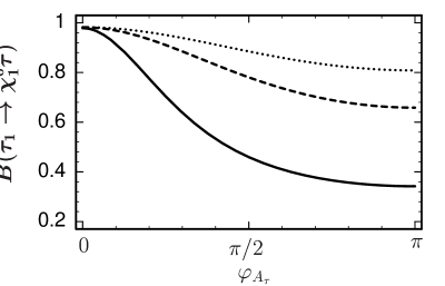
Figure 1: Branching ratio of $\tilde{\tau}_{1}\to\tilde{\chi}_{1}^{0}\tau$ as a function of $\varphi_{A_{\tau}}$ for $m_{\tilde{\tau}_{1}}=240$ GeV, $m_{\tilde{\nu}_{\tau}}=233$ GeV $(\rm solid~{}line)$, $238$ GeV $(\rm dashed~{}line)$, $243$ GeV $(\rm dotted~{}line)$, and $\varphi_{\mu}=\varphi_{U(1)}=0$, $|\mu|=300$ GeV, $|A_{\tau}|=1000$ GeV, $\tan\beta=3$, and $M_{2}=200$ GeV.

In this subsection we study the dependence of the branching ratios of $\tilde{\tau}_{1}$ decays into charginos and neutralinos on the phases $\varphi_{A_{\tau}}$, $\varphi_{\mu}$ and $\varphi_{U(1)}$. We take $m_{\tilde{\tau}_{1}}=240$ GeV. In order not to vary too many parameters we fix $|A_{\tau}|=1000$ GeV in Figs. 1 to 7. We assume the GUT relation $|M_{1}|=(5/3)\tan^{2}\Theta_{W}M_{2}$, although we take $M_{1}$ complex. We focus on the decays $\tilde{\tau}_{1}\rightarrow\tilde{\chi}^{0}_{1,2}\tau$ and $\tilde{\tau}_{1}\rightarrow\tilde{\chi}^{-}_{1}\nu_{\tau}$.

We first study the $\varphi_{A_{\tau}}$ dependence of the $\tilde{\tau}_{1}$ decay branching ratios, because $\varphi_{A_{\tau}}$ appears only in the $\tilde{\tau}_{i}$ sector and it is the phase dependence that we are particularly interested in. In Fig. 1 we plot the branching ratio $B(\tilde{\tau}_{1}\rightarrow\tilde{\chi}^{0}_{1}\tau)$ as a function of $\varphi_{A_{\tau}}$ for the three values $m_{\tilde{\nu}_{\tau}}=233$ GeV, $238$ GeV and $243$ GeV (corresponding to $M_{\tilde{L}}=240$ GeV, $245$ GeV and $250$ GeV), taking $\varphi_{\mu}=\varphi_{U(1)}=0$, $|\mu|=300$ GeV, $\tan\beta=3$, and $M_{2}=200$ GeV. Note that $B(\tilde{\tau}_{1}\rightarrow\tilde{\chi}^{0}_{1}\tau)$ is invariant under $\varphi_{A_{\tau}}\to-\varphi_{A_{\tau}}$ for $\varphi_{\mu}=\{0,\pm\pi\}$ and $\varphi_{U(1)}=\{0,\pm\pi\}$. As can be seen, the $\varphi_{A_{\tau}}$ dependence of $B(\tilde{\tau}_{1}\rightarrow\tilde{\chi}^{0}_{1}\tau)$ is quite pronounced. To a large extend it is caused by a relatively strong variation of the mixing angle $\theta_{\tilde{\tau}}$ with varying $\varphi_{A_{\tau}}$. More specifically, when varying $\varphi_{A_{\tau}}$ from $0$ to $\pi$, then $\cos\theta_{\tilde{\tau}}$ varies from $-0.1$ to $-0.9$ for $m_{\tilde{\nu}_{\tau}}=233$ GeV, from $-0.06$ to $-0.6$ for $m_{\tilde{\nu}_{\tau}}=238$ GeV and from $-0.05$ to $-0.45$ for $m_{\tilde{\nu}_{\tau}}=243$ GeV. This means that for $m_{\tilde{\nu}_{\tau}}=238$ GeV and $243$ GeV $\tilde{\tau}_{1}$ is mainly $\tilde{\tau}_{R}$-like, whereas for $m_{\tilde{\nu}_{\tau}}=233$ GeV $\tilde{\tau}_{1}$ is $\tilde{\tau}_{L}$-like ($\tilde{\tau}_{R}$-like) for $\varphi_{A_{\tau}}\;\raisebox{-3.87495pt}{$\textstyle\stackrel{{\scriptstyle\textstyle>}}{{\sim}}$}\;\pi/3(\;\raisebox{-3.87495pt}{$\textstyle\stackrel{{\scriptstyle\textstyle<}}{{\sim}}$}\;\pi/3)$. Such a strong variation of the mixing angle $\theta_{\tilde{\tau}}$ with $\varphi_{A_{\tau}}$ can only occur if $M_{\tilde{L}}\approx M_{\tilde{E}}$ and $|A_{\tau}|\approx|\mu|\tan\beta$, otherwise this variation is weaker.

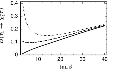
Figure 2: Branching ratio of $\tilde{\tau}_{1}\to\tilde{\chi}_{1}^{0}\tau$ as a function of $\tan\beta$ for $m_{\tilde{\tau}_{1}}=240$ GeV, $m_{\tilde{\tau}_{2}}=500$ GeV, $\varphi_{\mu}=0(\rm solid~{}line)$, $\pi/2(\rm dashed~{}line)$, $\pi(\rm dotted~{}line)$, with the other parameters $\varphi_{A_{\tau}}=\varphi_{U(1)}=0$, $M_{2}=200$ GeV, $|\mu|=150$ GeV, and $|A_{\tau}|=1000$ GeV, assuming $M_{\tilde{L}}<M_{\tilde{E}}$.

In the following Figs. 2 to 5 we fix $m_{\tilde{\tau}_{2}}=500$ GeV instead of $m_{\tilde{\nu}_{\tau}}$. We consider separately the two cases $M_{\tilde{L}}<M_{\tilde{E}}$ and $M_{\tilde{L}}\geq M_{\tilde{E}}$ and determine the values of $M_{\tilde{L}}$ and $M_{\tilde{E}}$ correspondingly. In Fig. 2 we show the $\tan\beta$ dependence of $B(\tilde{\tau}_{1}\rightarrow\tilde{\chi}^{0}_{1}\tau)$ for $\varphi_{\mu}=0$ (solid line), $\varphi_{\mu}=\pi/2$ (dashed line), $\varphi_{\mu}=\pi$ (dotted line), with $\varphi_{A_{\tau}}=\varphi_{U(1)}=0$, $M_{2}=200$ GeV, $|\mu|=150$ GeV, assuming $M_{\tilde{L}}<M_{\tilde{E}}$. For $\varphi_{A_{\tau}}=\{0,\pm\pi\}$ the branching ratios are invariant under the simultaneous sign flip $(\varphi_{\mu},\varphi_{U(1)})\to(-\varphi_{\mu},-\varphi_{U(1)})$. As can be seen, $B(\tilde{\tau}_{1}\rightarrow\tilde{\chi}^{0}_{1}\tau)$ becomes almost independent of $\varphi_{\mu}$ for $\tan\beta\raise 1.29167pt\hbox{$>$\kern-7.5pt\lower 4.30554pt\hbox{$\sim$}}15$. A similar behaviour is obtained for $B(\tilde{\tau}_{1}\rightarrow\tilde{\chi}^{0}_{2}\tau)$ and $B(\tilde{\tau}_{1}\rightarrow\tilde{\chi}^{-}_{1}\nu_{\tau})$. In the case of the decay $\tilde{\tau}_{1}\rightarrow\tilde{\chi}^{-}_{1}\nu_{\tau}$ this behaviour can be understood by observing that the $\varphi_{\mu}$ dependence of the mass eigenvalues $m_{\tilde{\chi}^{\pm}_{i}}$ and the mixing matrices $U_{ij}$ and $V_{ij}$ changes if the value of $\tan\beta$ is changed. For the width $\Gamma(\tilde{\tau}_{1}\rightarrow\tilde{\chi}^{-}_{1}\nu_{\tau})\propto|\ell^{\tilde{\tau}}_{11}|^{2}$ we obtain from Eqs. (6), (14), (15) and (40)

$$\ell^{\tilde{\tau}}_{11}=-e^{i\gamma_{1}}(e^{-i\varphi_{\tilde{\tau}}}\cos\theta_{\tilde{\tau}}\cos\theta_{1}-e^{i\phi_{1}}Y_{\tau}\sin\theta_{\tilde{\tau}}\sin\theta_{1}).$$

By inspecting Eqs. (5) and (44) one can verify that in the limit $\tan\beta\to\infty$ we obtain $e^{-i\varphi_{\tilde{\tau}}}\to-e^{i\varphi_{\mu}}$ and $e^{i\phi_{1}}\to e^{i\varphi_{\mu}}$, which means that in this limit $|\ell^{\tilde{\tau}}_{11}|$ becomes independent of $\varphi_{\mu}$. Here note that in this limit $\theta_{\tilde{\tau}}$ and $\theta_{1}$ become independent of $\varphi_{\mu}$ as can be seen from Eqs. (4), (7), (8) and (42). In the case of the decay into a neutralino we can see the influence of the phases $\varphi_{\mu}$ and $\varphi_{U(1)}$ from the approximate formulae

$$m_{\tilde{\chi}_{1}^{0}}\simeq|M_{1}|\left(1-\frac{m_{Z}^{2}\sin^{2}\Theta_{W}\sin 2\beta\cos(\varphi_{\mu}+\varphi_{U(1)})}{|\mu||M_{1}|}\right)$$ (31)

and

$$m_{\tilde{\chi}_{1}^{0}}\simeq|\mu|\left(1-\frac{m_{Z}^{2}}{2|\mu|}\Bigg{\{}\left[\frac{\sin^{2}\Theta_{W}}{|M_{1}|}+\frac{\cos^{2}\Theta_{W}}{M_{2}}\right]+\sin 2\beta\left[\frac{\sin^{2}\Theta_{W}\cos(\varphi_{\mu}+\varphi_{U(1)})}{|M_{1}|}+\frac{\cos^{2}\Theta_{W}\cos\varphi_{\mu}}{M_{2}}\right]\Bigg{\}}\right),$$ (32)

which hold for $|M_{2}\pm|\mu||\gg m_{Z}$ for the mass of a gaugino–like or a higgsino–like $\chi^{0}_{1}$, respectively. Similar approximation formulae hold for $m_{\tilde{\chi}^{0}_{2}}$ and the mixing matrix $N_{ij}$. From these formulae one can see that $\varphi_{\mu}$ and $\varphi_{U(1)}$ appear only in terms multiplied by $\sin 2\beta$. Therefore, in the approximation where Eqs. (31) and (32) hold, $m_{\tilde{\chi}^{0}_{1,2}}$ and $N_{ij}$ become independent of $\varphi_{\mu}$ and $\varphi_{U(1)}$ for large $\tan\beta$. Concerning the $\varphi_{\mu}$ dependence in general, it can be shown that $m_{\tilde{\chi}^{0}_{i}}$ and $N_{ij}$ become independent of $\varphi_{\mu}$ for $\tan\beta\to\infty$, because the characteristic equation of the neutralino mass eigenvalues becomes independent of $\varphi_{\mu}$ in this limit.

In Figs. 3 a, b we plot the branching ratio $B(\tilde{\tau}_{1}\rightarrow\tilde{\chi}^{0}_{1}\tau)$ against $M_{2}$ in the range $200$ GeV $\leq M_{2}\leq 500$ GeV for $\varphi_{\mu}=\pi$ (solid line), $\varphi_{\mu}=\pi/2$ (dashed line), $\varphi_{\mu}=0$ (dotted line) and $\varphi_{\mu}=-\pi/2$ (dash-dotted line), taking $\varphi_{A_{\tau}}=0$, $\varphi_{U(1)}=\pi/2$, $|\mu|=150$ GeV and $\tan\beta=3$. In Fig. 3 a we assume $M_{\tilde{L}}<M_{\tilde{E}}$, so that $\tilde{\tau}_{1}\simeq\tilde{\tau}_{L}(\cos\theta_{\tilde{\tau}}\approx-1)$. This means that the couplings are approximately $|a_{1j}^{\tilde{\tau}}|\simeq|f^{\tau}_{Lj}|$, $|b_{1j}^{\tilde{\tau}}|\simeq|h^{\tau}_{Lj}|$ and the decay width is essentially determined by $\Gamma(\tilde{\tau}_{1}\rightarrow\tilde{\chi}^{0}_{j}\tau)\propto|f^{\tau}_{Lj}|^{2}+|h^{\tau}_{Lj}|^{2}$. In Fig. 3 b we consider the case $M_{\tilde{L}}\geq M_{\tilde{E}}$. In this case we have $|a_{1j}^{\tilde{\tau}}|\simeq|h^{\tau}_{Rj}|$, $|b_{1j}^{\tilde{\tau}}|\simeq|f^{\tau}_{Rj}|$ and $|\ell_{1j}^{\tilde{\tau}}|\simeq Y_{\tau}|U_{j2}|$. This means that the decay $\tilde{\tau}_{1}\rightarrow\tilde{\chi}_{1}^{-}\nu_{\tau}$ is suppressed, because now $\tilde{\tau}_{1}\simeq\tilde{\tau}_{R}$ ($\cos\theta_{\tilde{\tau}}\approx 0$) and the $\tilde{\tau}_{1}\tilde{\chi}_{1}^{-}\nu_{\tau}$ coupling is nearly proportional to the small Yukawa coupling $Y_{\tau}$. Therefore, $B(\tilde{\tau}_{1}\rightarrow\tilde{\chi}^{0}_{1}\tau)$ in Fig. 3 b is larger than in Fig. 3 a. In both cases there is a significant variation with $\varphi_{\mu}$. The $\varphi_{\mu}$ dependence of $B(\tilde{\tau}_{1}\rightarrow\tilde{\chi}^{0}_{1}\tau)$ in Figs. 3 a, b is caused by an interplay between the $\varphi_{\mu}$ dependence of the mass and mixing character of the $\tilde{\tau}_{1}$ and that of the $\tilde{\chi}^{0}_{1}$. The $M_{2}$ dependence can be understood by noting that for $M_{2}\approx 200$ GeV the lightest neutralino has a sizable gaugino content, which decreases for increasing $M_{2}$. For our parameter choice $\tilde{\chi}^{0}_{1}$ becomes mainly higgsino–like for $M_{2}\raise 1.29167pt\hbox{$>$\kern-7.5pt\lower 4.30554pt\hbox{$\sim$}}300$ GeV. Near $M_{2}\approx 440$ GeV the decays into gaugino–like neutralinos become kinematically forbidden, which causes the increase of $B(\tilde{\tau}_{1}\rightarrow\tilde{\chi}^{0}_{1}\tau)$ for $M_{2}\raise 1.29167pt\hbox{$>$\kern-7.5pt\lower 4.30554pt\hbox{$\sim$}}400$ GeV.

We have studied the $\varphi_{\mu}$ dependence of $B(\tilde{\tau}_{1}\rightarrow\tilde{\chi}^{0}_{1}\tau)$ also for other values of $|\mu|$ and have found that it is less pronounced if $|\mu|\raise 1.29167pt\hbox{$>$\kern-7.5pt\lower 4.30554pt\hbox{$\sim$}}M_{2}$ and that it is stronger if $|\mu|\approx M_{2}$ or $|\mu|\raise 1.29167pt\hbox{$<$\kern-7.5pt\lower 4.30554pt\hbox{$\sim$}}|M_{1}|$. As shown in Fig. 2 it is stronger for low $\tan\beta$.

In Figs. 4 a, b we show the $\varphi_{U(1)}$ dependence of $B(\tilde{\tau}_{1}\rightarrow\tilde{\chi}^{0}_{1}\tau)$ for $|\mu|=150$ GeV, $\tan\beta=3$ and $\varphi_{A_{\tau}}=0$, for $\varphi_{\mu}=\pi$ (solid line), $\varphi_{\mu}=\pi/2$ (dashed line), $\varphi_{\mu}=0$ (dotted line) and $\varphi_{\mu}=-\pi/2$ (dash-dotted line). In Fig. 4 a we take $M_{\tilde{L}}<M_{\tilde{E}}$ and $M_{2}=280$ GeV. Fig. 4 b is for $M_{\tilde{L}}\geq M_{\tilde{E}}$ and $M_{2}=380$ GeV. Although the $\varphi_{U(1)}$ dependence of $B(\tilde{\tau}_{1}\rightarrow\tilde{\chi}^{0}_{1}\tau)$ stems only from the $\varphi_{U(1)}$ dependence of the $\tilde{\chi}^{0}_{1,2}$ parameters, it is quite pronounced. It is essentially explained by the $\varphi_{U(1)}$ dependences of $N_{11}$ and $N_{12}$, which enter in the couplings $f^{\tau}_{L1}$ and $f^{\tau}_{R1}$ (see Eqs. (14) – (16)). For example, the minimum of $B(\tilde{\tau}_{1}\rightarrow\tilde{\chi}^{0}_{1}\tau)$ in Fig. 4 b at $\varphi_{U(1)}\approx 3\pi/4~{}(-3\pi/4)$ for $\varphi_{\mu}=\pi/2~{}(-\pi/2)$ is caused by a corresponding minimum of $|N_{11}|$.

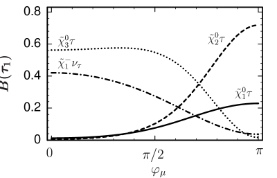
Figure 5: Branching ratios of $\tilde{\tau}_{1}\to\tilde{\chi}^{0}_{1,2,3}\tau$ and $\tilde{\tau}_{1}\to\tilde{\chi}^{-}_{1}\nu_{\tau}$ as a function of $\varphi_{\mu}$ for $\varphi_{U(1)}=\varphi_{A_{\tau}}=0$, $m_{\tilde{\tau}_{1}}=240$ GeV, $m_{\tilde{\tau}_{2}}=500$ GeV, $M_{2}=280$ GeV, $|\mu|=150$ GeV, $\tan\beta=3$, and $|A_{\tau}|=1000$ GeV, assuming $M_{\tilde{L}}<M_{\tilde{E}}$.

We have also studied how the branching ratios $B(\tilde{\tau}_{1}\rightarrow\tilde{\chi}^{0}_{2,3}\tau)$ and $B(\tilde{\tau}_{1}\rightarrow\tilde{\chi}^{-}_{1}\nu_{\tau})$ vary as functions of the phases. As an example we show in Fig. 5 these branching ratios as functions of $\varphi_{\mu}$ for $\varphi_{U(1)}=\varphi_{A_{\tau}}=0$, $M_{2}=280$ GeV, $|\mu|=150$ GeV and $\tan\beta=3$, assuming $M_{\tilde{L}}<M_{\tilde{E}}$. For this set of parameters all branching ratios shown have a significant $\varphi_{\mu}$ dependence. Their behaviour can be understood in the following way: If we first consider $B(\tilde{\tau}_{1}\rightarrow\tilde{\chi}^{-}_{1}\nu_{\tau})\propto|U_{11}|^{2}$, the $\varphi_{\mu}$ dependence of $|U_{11}|$ follows from

$$|U_{11}|^{2}=\cos^{2}\theta_{1}=\frac{1}{2}\left(1+\frac{|\mu|^{2}-M_{2}^{2}+2m_{W}^{2}\cos 2\beta}{m_{\tilde{\chi}^{+}_{2}}^{2}-m_{\tilde{\chi}^{+}_{1}}^{2}}\right),$$ (33)

where $\theta_{1}$ is the mixing angle of the chargino mixing matrix $U_{ij}$ defined in Eq. (42). The mass squared difference $m_{\tilde{\chi}^{+}_{2}}^{2}-m_{\tilde{\chi}^{+}_{1}}^{2}$ decreases for $\varphi_{\mu}\to\pi$, which can be seen from Eq. (48), therefore, also $|U_{11}|$ decreases. The behaviour of $B(\tilde{\tau}_{1}\rightarrow\tilde{\chi}^{0}_{1,2,3}\tau)$ can be understood by noting that $\tilde{\chi}^{0}_{1,2,3}$ have large higgsino–components. Varying $\varphi_{\mu}$ from $0$ to $\pi$ essentially interchanges the $\tilde{H}^{0}_{1}$ and $\tilde{H}^{0}_{2}$ components of $\tilde{\chi}^{0}_{1,2,3}$. This causes the variation in the branching ratios, because $\tilde{\tau}_{1}$ couples to the $\tilde{H}_{1}^{0}$ component of $\tilde{\chi}^{0}_{i}$ but not to the $\tilde{H}^{0}_{2}$ component.

It is expected that $\varphi_{\mu}$ and $\varphi_{U(1)}$ will be determined by measuring suitable observables of the chargino and neutralino sectors [27]. The $\varphi_{\mu}$ and $\varphi_{U(1)}$ dependences of the various $\tilde{\tau}_{1}$ decay branching ratios, however, will give useful additional information for the precise determination of $\varphi_{\mu}$ and $\varphi_{U(1)}$ and thereby provide further tests of the MSSM with complex parameters. This may also be helpful for resolving the ambiguities encountered in the studies about the parameter determination of the chargino and neutralino sectors [27].

An additional observable which is very sensitive to the SUSY parameters of the $\tilde{\tau}_{i}$ and ${\tilde{\chi}}^{0}_{k}$ systems is the longitudinal polarization of the outgoing $\tau$–lepton in the decays $\tilde{\tau}_{i}\rightarrow\tilde{\chi}^{0}_{j}\tau$ [25]. For the $\tilde{\tau}_{1}$ decays into neutralinos it is defined as

$$\mathcal{P}_{\tau}=\frac{B(\tilde{\chi}_{j}^{0}\tau_{R})-B(\tilde{\chi}_{j}^{0}\tau_{L})}{B(\tilde{\chi}_{j}^{0}\tau_{R})+B(\tilde{\chi}_{j}^{0}\tau_{L})}=\frac{|b_{1j}^{\tilde{\tau}}|^{2}-|a_{1j}^{\tilde{\tau}}|^{2}}{|b_{1j}^{\tilde{\tau}}|^{2}+|a_{1j}^{\tilde{\tau}}|^{2}}$$ (34)

where the last equation holds in the limit $m_{\tau}\rightarrow 0$. $R,L$ denote $\lambda_{\tau}=+\frac{1}{2},-\frac{1}{2}$, respectively.

We show in Figs. 6 a, b the longitudinal polarization of the $\tau$ in the decays $\tilde{\tau}_{1}\rightarrow\tilde{\chi}^{0}_{1}\tau$ and $\tilde{\tau}_{1}\rightarrow\tilde{\chi}^{0}_{2}\tau$, respectively, as a function of $\varphi_{A_{\tau}}$ for $m_{\tilde{\nu}_{\tau}}=233$ GeV (solid line), $238$ GeV (dashed line) and $243$ GeV (dotted line), which correspond to $M_{\tilde{L}}=240$ GeV, $245$ GeV and $250$ GeV, respectively. The other parameters are $M_{2}=200$ GeV, $|\mu|=300$ GeV, $\tan\beta=3$, $\varphi_{\mu}=\varphi_{U(1)}=0$. The behaviour of $\mathcal{P}_{\tau}(\tilde{\chi}^{0}_{1}\tau)$ in Fig. 6 a follows from the change of the mixing angle $\theta_{\tilde{\tau}}$ with varying $\varphi_{A_{\tau}}$, as described in the discussion of Fig. 1. The behaviour of $\mathcal{P}_{\tau}(\tilde{\chi}^{0}_{2}\tau)$ in Fig. 6 b can be understood by noting that in this case $\tilde{\chi}^{0}_{2}$ is mainly a $\tilde{W}^{3}$ which couples only to the $\tilde{\tau}_{L}$ component of $\tilde{\tau}_{1}$ and that this component strongly increases for $\varphi_{A_{\tau}}\to\pi$ as can be seen from Eqs. (6) and (7).

In Fig. 7 we show the longitudinal $\tau$ polarization in the decays $\tilde{\tau}_{1}\to\tilde{\chi}^{0}_{1}\tau$ and $\tilde{\tau}_{1}\to\tilde{\chi}^{0}_{2}\tau$ as a function of $\varphi_{\mu}$. Here we have taken $m_{\tilde{\tau}_{2}}=500$ GeV and the other parameters $M_{2}=350$ GeV, $|\mu|=150$ GeV, $\tan\beta=3$, $\varphi_{U(1)}=\varphi_{A_{\tau}}=0$. As we have chosen $M_{\tilde{L}}<M_{\tilde{E}}$, $\tilde{\tau}_{1}$ is mainly a $\tilde{\tau}_{L}$ and $\mathcal{P}_{\tau}$ is negative for $\varphi_{\mu}\;\raisebox{-3.87495pt}{$\textstyle\stackrel{{\scriptstyle\textstyle>}}{{\sim}}$}\;3\pi/10$ due to the very small $\tau$ Yukawa coupling. For $\varphi_{\mu}\rightarrow 0$, the $\tilde{\tau}_{L}\tau_{L}\tilde{\chi}^{0}_{1,2}$ couplings $|f^{\tau}_{L1}|$ and $|f^{\tau}_{L2}|$ decrease monotonically, because $\tilde{\chi}^{0}_{1,2}$ are mainly higgsino-like and changing the phase $\varphi_{\mu}$ from $\pi$ to $0$ implies essentially a decrease of their gaugino components as well as exchanging the ${\tilde{H}}^{0}_{1}$ component with the ${\tilde{H}}^{0}_{2}$ component. This leads to a change of the sign of $\mathcal{P}_{\tau}$. $|f^{\tau}_{L2}|$ has a maximum at $\varphi_{\mu}\approx 3\pi/4$, which is clearly seen in the minimum of $\mathcal{P}_{\tau}(\tilde{\chi}_{2}^{0}\tau)\approx-0.6$ for this value of $\varphi_{\mu}$.

4.2 $\tilde{\tau}_{2}$ Decays

As we have seen in the previous subsection, the branching ratios for the fermionic $\tilde{\tau}_{1}$ decays depend on the phase $\varphi_{A_{\tau}}$ only via the $\cos(\varphi_{A_{\tau}}+\varphi_{\mu})$ dependence of the mass $m_{\tilde{\tau}_{1}}$ and the mixing angle $\theta_{\tilde{\tau}}$. We consider now the bosonic $\tilde{\tau}_{2}$ decays where the couplings to the Higgs bosons explicitely depend on the phases $\varphi_{A_{\tau}}$ and $\varphi_{\mu}$ (see Eqs. (25) to (30)). The decay widths into $W^{\pm}$, $Z$ and Higgs bosons are enhanced by choosing $|\mu|$ and/or $|A_{\tau}|$ large [28].

As already mentioned, the RG improved Higgs sector is determined by the parameters $m_{H^{\pm}}$, $\tan\beta$, $|\mu|$, $|A_{t}|$, $|A_{b}|$, $\varphi_{\mu}$, $\varphi_{A_{t}}$, $\varphi_{A_{b}}$, $M_{\tilde{Q}}$, $M_{\tilde{U}}$, $M_{\tilde{D}}$, $|m_{\tilde{g}}|$, $\varphi_{\tilde{g}}$, $|M_{1}|$, $\varphi_{U(1)}$ and $M_{2}$ [15]. We fix $M_{\tilde{Q}}=M_{\tilde{U}}=M_{\tilde{D}}=M_{SUSY}$. The amount of the $CP$ violating scalar–pseudoscalar transition in the neutral Higgs mass matrix is proportional to the parameter

$$\eta_{CP}=\frac{g^{2}m^{4}_{f}|A_{f}||\mu|}{128\pi^{2}m_{W}^{2}M^{2}_{SUSY}}\sin(\varphi_{\mu}+\varphi_{A_{f}}),$$ (35)

where $f=t,b$ [15, 16]. This means that significant $CP$ violating effects in the Higgs sector can be expected if $|\mu|,|A_{f}|>M_{SUSY}$ and $|\sin(\varphi_{\mu}+\varphi_{A_{f}})|\approx 1$. As we focus on the $\varphi_{A_{\tau}}$ and the $\varphi_{\mu}$ dependence of the observables, we fix the phases $\varphi_{A_{t}}=\varphi_{\tilde{g}}=0$, $\varphi_{A_{b}}=\pi$ and we take $|A_{t}|=|A_{b}|=800$ GeV, $M_{SUSY}=600$ GeV, $|m_{\tilde{g}}|=(\alpha_{s}(|m_{\tilde{g}}|)/\alpha_{2})M_{2}$ (with $\alpha_{s}(Q)=12\pi/((33-2n_{f})\ln(Q^{2}/\Lambda^{2}_{n_{f}}))$, $n_{f}$ being the number of quark flavors). For this choice of parameters mixing between the CP–even and CP–odd Higgs bosons at one loop level occurs only if $\varphi_{\mu}\neq\{0,\pm\pi\}$. Therefore, we can control the influence of explicit CP violation in the Higgs sector with the parameter $\varphi_{\mu}$. With this choice of parameters the constraint from the $\rho$-parameter on the $\tilde{t}$ and $\tilde{b}$ masses and mixings, $\delta\rho(\tilde{t}-\tilde{b})<0.0012$, is always fulfilled [29].

For large $\tan\beta$ the allowed range of $|\mu|$ is restricted by the two-loop contributions to the EDMs of electron and neutron [30]. For example, for $\tan\beta=40$, $\varphi_{\mu}=\pi/2$, $m_{H^{\pm}}\raise 1.29167pt\hbox{$<$\kern-7.5pt\lower 4.30554pt\hbox{$\sim$}}200$ GeV and the other parameters as fixed above the EDMs give the restriction $|\mu|\raise 1.29167pt\hbox{$<$\kern-7.5pt\lower 4.30554pt\hbox{$\sim$}}600$ GeV. Therefore, we also fix $|\mu|=600$ GeV.

In the following we give some numerical examples which show the dependence of the branching ratios for $\tilde{\tau}_{2}\to\tilde{\tau}_{1}H_{i},i=1,2,3,$ on $\varphi_{A_{\tau}}$, $\tan\beta$ and $m_{H^{\pm}}$. We take $|A_{\tau}|=900$ GeV, $M_{2}=450$ GeV and $\varphi_{U(1)}=0$. We consider the case $M_{\tilde{L}}>M_{\tilde{E}}$, where $\tilde{\tau}_{2}$ is mainly $\tilde{\tau}_{L}$-like and $\tilde{\tau}_{1}$ is mainly $\tilde{\tau}_{R}$-like. In this case the decays $\tilde{\tau}_{2}\to W^{-}\tilde{\nu}_{\tau}$ and $\tilde{\tau}_{2}\to H^{-}\tilde{\nu}_{\tau}$ are kinematically forbidden.

In Figs. 8 a, b we show the branching ratios for various fermionic and bosonic $\tilde{\tau}_{2}$ decays as a function of $\varphi_{A_{\tau}}$ for $\varphi_{\mu}=0$ and $\pi/2$, taking $\tan\beta=30$, $m_{H^{\pm}}=160$ GeV, $m_{\tilde{\tau}_{1}}=240$ GeV, $m_{\tilde{\tau}_{2}}=500$ GeV and the other parameters as specified above. As can be seen, the branching ratios of the decays $\tilde{\tau}_{2}\to H_{1,2,3}\tilde{\tau}_{1}$ show a pronounced ($\varphi_{A_{\tau}}$,$\varphi_{\mu})$ dependence. The behaviour of these branching ratios can be understood by examining the approximate formula for the coupling squared for $\tilde{\tau}_{2}\to\tilde{\tau}_{1}H_{i},$

$$|C(\tilde{\tau}_{2}^{\ast}H_{i}\tilde{\tau}_{1})|^{2}\simeq|C(\tilde{\tau}_{L}^{\ast}H_{i}\tilde{\tau}_{R})|^{2}\left(1-2\sin^{2}\theta_{\tilde{\tau}}\cos^{2}\theta_{\tilde{\tau}}(1+\cos 2(\arg[C(\tilde{\tau}_{L}^{\ast}H_{i}\tilde{\tau}_{R})]+\varphi_{\tilde{\tau}}))\right)$$ (36)

with

$$|C(\tilde{\tau}_{L}^{\ast}H_{i}\tilde{\tau}_{R})|^{2} \simeq \frac{1}{2}Y_{\tau}^{2}\biggl{(}\Bigl{(}|\mu|^{2}-|A_{\tau}|^{2}\Bigr{)}\mathcal{O}_{2i}^{2}+|A_{\tau}|^{2}-2|\mu||A_{\tau}|\mathcal{O}_{2i}$$ (37)

$${}\times\Bigl{(}\mathcal{O}_{1i}\cos(\varphi_{A_{\tau}}+\varphi_{\mu})-\mathcal{O}_{3i}\sin(\varphi_{A_{\tau}}+\varphi_{\mu})\Bigr{)}\biggr{)},$$

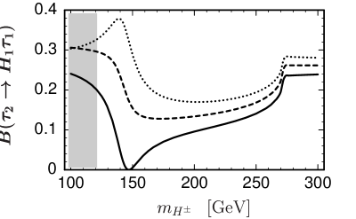
Figure 9: Branching ratio of $\tilde{\tau}_{2}\to H_{1}\tilde{\tau}_{1}$, as a function of $m_{H^{\pm}}$ for $\varphi_{A_{\tau}}=0(\rm solid~{}line)$, $\pi/2(\rm dashed~{}line)$, $\pi(\rm dotted~{}line)$, $\varphi_{\mu}=\varphi_{U(1)}=0$, $m_{\tilde{\tau}_{1}}=240$ GeV, $m_{\tilde{\tau}_{2}}=500$ GeV, $|\mu|=600$ GeV, $|A_{\tau}|=900$ GeV, $\tan\beta=30$, and $M_{2}=450$ GeV, assuming $M_{\tilde{L}}>M_{\tilde{E}}$. In the grey area the condition $m_{H_{1}}>110$ GeV is not fulfilled.

which follows from Eq. (28) and (30). Here we have omitted terms proportional to $(C(\tilde{\tau}_{L}^{\ast}H_{i}\tilde{\tau}_{L})-C(\tilde{\tau}_{R}^{\ast}H_{i}\tilde{\tau}_{R}))$ and $\cos\beta$. Eqs. (36) and (37) show that a significant phase dependence of the $\tilde{\tau}_{2}\to\tilde{\tau}_{1}H_{i}$ branching ratios can be expected for large $\tan\beta$. Moreover, also the $\varphi_{\mu}$ dependence of the Higgs mixing matrix elements $\mathcal{O}_{ij}$ influences in a significant way the behaviour of $B(\tilde{\tau}_{2}\to\tilde{\tau}_{1}H_{i})$. For $\varphi_{\mu}=0$, for example, we obtain $\mathcal{O}_{11}\approx-0.262$, $\mathcal{O}_{21}\approx-0.965$, $\mathcal{O}_{31}=\mathcal{O}_{12}=\mathcal{O}_{22}=0$, $\mathcal{O}_{32}=1$, $\mathcal{O}_{13}\approx 0.965$, $\mathcal{O}_{23}\approx-0.262$, $\mathcal{O}_{33}=0$, $m_{H_{1}}=115.74$ GeV, $m_{H_{2}}=138.48$ GeV, $m_{H_{3}}=139.14$ GeV. The $\varphi_{A_{\tau}}$ dependence of $B(\tilde{\tau}_{2}\to H_{1}\tilde{\tau}_{1})$ follows essentially from the $\cos(\varphi_{A_{\tau}}+\varphi_{\mu})$ term and the first two terms of Eq. (37). The minimum of $B(\tilde{\tau}_{2}\to H_{1}\tilde{\tau}_{1})$ at $\varphi_{A_{\tau}}=0$ (Fig. 8 a) follows from a partial cancellation of the terms in Eq. (37) (or, equivalently, from a partial cancellation of the last two terms of Eq. (28), see also Fig. 9 below). The $\cos(\varphi_{A_{\tau}}+\varphi_{\mu})$ term and the first two terms of Eq. (37) determine also the $\varphi_{A_{\tau}}$ behaviour of $B(\tilde{\tau}_{2}\to H_{3}\tilde{\tau}_{1})$. The $\varphi_{A_{\tau}}$ dependence of $B(\tilde{\tau}_{2}\to H_{2}\tilde{\tau}_{1})$ follows from the last factor of Eq. (36) and the first term of Eq. (28). As for Fig. 8 b, for $\varphi_{\mu}=\pi/2$ we obtain $\mathcal{O}_{11}\approx-0.106$, $\mathcal{O}_{21}\approx-0.992$, $\mathcal{O}_{31}\approx 0.066$, $\mathcal{O}_{12}\approx-0.230$, $\mathcal{O}_{22}\approx-0.040$, $\mathcal{O}_{32}\approx-0.972$, $\mathcal{O}_{13}\approx 0.967$, $\mathcal{O}_{23}\approx-0.118$, $\mathcal{O}_{33}\approx-0.224$, $m_{H_{1}}=117.09$ GeV, $m_{H_{2}}=138.48$ GeV, $m_{H_{3}}=139.14$ GeV. The $\varphi_{A_{\tau}}$ dependence of $B(\tilde{\tau}_{2}\to H_{i}\tilde{\tau}_{1})$ is now different from that in Fig. 8 a. In the case of $B(\tilde{\tau}_{2}\to H_{1}\tilde{\tau}_{1})$ the $\cos(\varphi_{A_{\tau}}+\varphi_{\mu})$ term becomes $-\sin\varphi_{A_{\tau}}$ and it is multiplied by a much smaller factor, which explains the relatively flat $\varphi_{A_{\tau}}$ dependence. The behaviour of $B(\tilde{\tau}_{2}\to H_{2}\tilde{\tau}_{1})$ and $B(\tilde{\tau}_{2}\to H_{3}\tilde{\tau}_{1})$ can be explained in an analogous way. For comparison we also plotted the branching ratios of $\tilde{\tau}_{2}\to Z\tilde{\tau}_{1}$ and of some of the decays into charginos and neutralinos. The $\varphi_{A_{\tau}}$ dependence of $\tilde{\tau}_{2}\to Z\tilde{\tau}_{1}$ essentially drops out (see Eq. (10)) and that of the fermionic decays disappears due to the large value of $\tan\beta$ for which $\theta_{\tilde{\tau}}$ is insensitive to $\varphi_{A_{\tau}}$.

We also studied the $\tan\beta$ dependence and the $m_{H^{\pm}}$ dependence of the $\tilde{\tau}_{2}$ decay branching ratios into neutral Higgs particles. For $\tan\beta\to 0$ these branching ratios vanish ($\propto\tan\beta$), whereas for $\tan\beta>10$ they depend only weakly on $\tan\beta$. The $m_{H^{\pm}}$ dependence of the branching ratio $B(\tilde{\tau}_{2}\to H_{1}\tilde{\tau}_{1})$ is shown in Fig. 9 for $\varphi_{A_{\tau}}=0,\pi/2,\pi$. At $m_{H^{\pm}}=150$ GeV and $\varphi_{A_{\tau}}=0$ this branching ratio practically vanishes. The reason is that the coupling $C(\tilde{\tau}_{L}^{\ast}H_{1}\tilde{\tau}_{R})$ practically vanishes for this set of parameters due to a cancellation of the last two terms in Eq. (28). At this point also a level crossing of $H_{1}$ and $H_{2}$ occurs. We see that this branching ratio is sensitive to $\varphi_{A_{\tau}}$ for $m_{H^{\pm}}\;\raisebox{-3.87495pt}{$\textstyle\stackrel{{\scriptstyle\textstyle<}}{{\sim}}$}\;250$ GeV.

4.3 $\tilde{\nu}_{\tau}$ Decays

The decay widths for $\tilde{\nu}_{\tau}$ decays into charginos and neutralinos are independent of $\varphi_{A_{\tau}}$. The decay widths for $\tilde{\nu}_{\tau}\to\tilde{\chi}^{+}_{k}\tau$ depend on $\varphi_{\mu}$, those for $\tilde{\nu}_{\tau}\to\tilde{\chi}^{0}_{k}\nu_{\tau}$ depend also on $\varphi_{U(1)}$. We first assume $M_{\tilde{L}}<M_{\tilde{E}}$, which leads to a sneutrino mass $m_{\tilde{\nu}_{\tau}}\simeq 229$ GeV for $m_{\tilde{\tau}_{1}}=240$ GeV, $m_{\tilde{\tau}_{2}}=500$ GeV and $\tan\beta=3$. In this case the decays $\tilde{\nu}_{\tau}\to W^{+}\tilde{\tau}_{1}$ and $\tilde{\nu}_{\tau}\to H^{+}\tilde{\tau}_{1}$ are kinematically forbidden.

We show in Figs. 10 a and b the branching ratios for the decays into $\tilde{\chi}^{0}_{1}\nu_{\tau}$, $\tilde{\chi}^{0}_{2}\nu_{\tau}$ and $\tilde{\chi}^{+}_{1}\tau$ as functions of $\varphi_{\mu}$ and $\varphi_{U(1)}$, respectively, for $M_{2}=500$ GeV, $|\mu|=150$ GeV, $\tan\beta=3$, and $|A_{\tau}|=1000$ GeV. In Fig. 10 a we take $\varphi_{U(1)}=0$ and in Fig. 10 b we take $\varphi_{\mu}=0$. As can be seen, the branching ratio for $\tilde{\nu}_{\tau}\to\tilde{\chi}^{0}_{1}\nu_{\tau}$ decreases for $\varphi_{\mu}\to\pi$, whereas those for $\tilde{\nu}_{\tau}\to\tilde{\chi}^{0}_{2}\nu_{\tau}$ and $\tilde{\nu}_{\tau}\to\tilde{\chi}^{+}_{1}\tau$ increase. The decay widths $\Gamma(\tilde{\nu}_{\tau}\to\tilde{\chi}_{1}^{0}\nu_{\tau})$ and $\Gamma(\tilde{\nu}_{\tau}\to\tilde{\chi}_{2}^{0}\nu_{\tau})$ decrease for $\varphi_{\mu}\to\pi$, because the matrix elements $|N_{12}|$ and $|N_{22}|$ decrease for $\varphi_{\mu}\to\pi$. The matrix element $|V_{11}|$ entering the decay width $\Gamma(\tilde{\nu}_{\tau}\to\tilde{\chi}_{1}^{+}\tau)$ also decreases, see Eqs. (41) and (43). However, as $\Gamma(\tilde{\nu}_{\tau}\to\tilde{\chi}_{1}^{+}\tau)$ and $\Gamma(\tilde{\nu}_{\tau}\to\tilde{\chi}_{2}^{0}\nu_{\tau})$ decrease more slowly than the total decay width, the corresponding branching ratios increase for $\varphi_{\mu}\to\pi$. In Fig. 10 b the branching ratio $B(\tilde{\nu}_{\tau}\to\tilde{\chi}_{1}^{0}\nu_{\tau})$ decreases for $\varphi_{U(1)}\to\pi$ and $B(\tilde{\nu}_{\tau}\to\tilde{\chi}_{1}^{+}\tau)$ increases. The reason is that $|N_{11}\tan\Theta_{W}-N_{12}|$ and hence the width $\Gamma(\tilde{\nu}_{\tau}\to\tilde{\chi}_{1}^{0}\nu_{\tau})$ rapidly decreases for $\varphi_{U(1)}\to\pi$. $B(\tilde{\nu}_{\tau}\to\tilde{\chi}_{1}^{+}\tau)$ increases due to the decrease of the total decay width.

In the case $M_{\tilde{L}}-M_{\tilde{E}}\raise 1.29167pt\hbox{$>$\kern-7.5pt\lower 4.30554pt\hbox{$\sim$}}m_{W},m_{H^{+}}$ also the bosonic decays $\tilde{\nu}_{\tau}\rightarrow W^{+}\tilde{\tau}_{1},H^{+}\tilde{\tau}_{1}$ are kinematically allowed. Consequently, the branching ratios of the fermionic decays are reduced. It turns out that in most cases the bosonic decay widths are almost independent of the phases; only in the region $|\mu|\ll m_{\tilde{\nu}_{\tau}}<|M_{1,2}|$ a significant dependence on the phases is possible. For small $\tan\beta$ the phase dependence of the width $\Gamma(\tilde{\nu}_{\tau}\rightarrow H^{+}\tilde{\tau}_{1})$ tends to be suppressed, because of the small Yukawa coupling, see Eq. (25). For large $\tan\beta$ the term $m_{\tau}A_{\tau}^{*}\tan\beta$ in Eq. (25) dominates and $\Gamma(\tilde{\nu}_{\tau}\rightarrow H^{+}\tilde{\tau}_{1})\propto$ $|\sin\theta_{\tilde{\tau}}C(\tilde{\nu}_{\tau}^{\ast}H^{+}\tilde{\tau}_{R})|^{2}\propto|\sin\theta_{\tilde{\tau}}m_{\tau}A^{*}_{\tau}\tan\beta|^{2}$ becomes essentially independent of the phases. Note here that $\theta_{\tilde{\tau}}$ is hardly sensitive to the phases because $M^{2}_{\tilde{L}}-M^{2}_{\tilde{E}}\gg m_{\tau}|A_{\tau}-\mu^{*}\tan\beta|$ in these scenarios. The phase dependence of the width $\Gamma(\tilde{\nu}_{\tau}\rightarrow W^{+}\tilde{\tau}_{1})$ is caused only by the phase dependence of $\cos\theta_{\tilde{\tau}}$ (see Eq. (24)) and is again weak by the same reasoning as above.

5 Parameter Determination

We now study the extent to which one can extract the underlying parameters from measured masses, branching ratios and cross sections. In the following we assume that an integrated luminosity of 2 ab^-1 is available. At a high luminosity collider like TESLA one can expect that this amount of integrated luminosity will be accumulated in four years of running [6]. Our strategy is as follows:

1. Take a specific set of values of the MSSM parameters.

2. Calculate the masses of $\tilde{\tau}_{i}$, $\tilde{\chi}^{0}_{j}$, $\tilde{\chi}^{\pm}_{k}$, the production cross sections for $e^{+}e^{-}\to\tilde{\tau}_{i}\overline{\tilde{\tau}}_{j}$ and branching ratios of the $\tilde{\tau}_{i}$ decays.

3. Regard these calculated values as real experimental data with definite errors.

4. Determine the underlying MSSM parameters and their errors from the “experimental data” by a fit.

We have checked that inclusion of the data on the mass, production and decays of $\tilde{\nu}_{\tau}$ does not further improve the accuracy of the underlying parameters to be determined. The reason is that the expected relative errors of the data in the sneutrino sector are larger than those in the stau sector [31, 32].

We have taken the following input parameters for the calculation of these observables: $M_{\tilde{E}}=$ 150 GeV, $M_{\tilde{L}}=$ 350 GeV, $A_{\tau}=$ -800 i GeV, $M_{2}=$ 280 GeV, $\mu=$ 250 GeV and $\varphi_{U(1)}=0$. We have considered the cases $\tan\beta=3$ and $30$. The Higgs sector has been fixed with $m_{H^{+}}=170$ GeV (160), $m_{A^{0}}=151.4$ GeV (138.5), $m_{h^{0}}=113.3$ GeV (115.7), $m_{H^{0}}=155.6$ GeV (139.1) and $\sin\alpha=0.432$ (-0.26) in case of $\tan\beta=3$ (30). Here $h^{0}$, $H^{0}$, $A^{0}$, $\alpha$ are the lighter CP-even Higgs boson, the heavier CP-even Higgs boson, the CP-odd Higgs boson and the mixing angle of the CP-even Higgs bosons, respectively. Here we focus on the determination of the phase $\varphi_{A_{\tau}}$ of $A_{\tau}$, therefore, we neglect mixing of the $CP$-even and $CP$-odd Higgs states. We have taken the relative errors of stau masses, chargino and neutralino masses from [6, 33], which we rescale according to our scenario; in case of $\tan\beta=30$ we have taken into account an additional factor of 3 for the errors (relatively to $\tan\beta=3$) due to the reduced efficiency in case of multi $\tau$ final states as indicated by the studies in [34]. We take the errors of the Higgs mass parameters as $\Delta m_{h^{0}}=50$ MeV, $\Delta m_{H^{0}}=\Delta m_{A^{0}}=\Delta m_{H^{+}}=1.5$ GeV [6] for $\tan\beta=3$ and 30. For the branching ratios and the production cross sections we have taken the statistical errors only. We give the values of the calculated masses and assumed errors in Table 1 and those of the calculated branching ratios of $\tilde{\tau}_{2}$ decays in Table 2. $\tilde{\tau}_{1}$ decays only into $\tau\tilde{\chi}^{0}_{1}$ for both values of $\tan\beta$, because this is the only channel open.

Table 1: Calculated masses and their assumed errors (in GeV).

$\tan\beta=3$		$\tan\beta=30$
$m_{\tilde{\tau}_{1}}=155.0\pm 0.7$	$m_{\tilde{\tau}_{2}}=352.6\pm 1.2$	$m_{\tilde{\tau}_{1}}=150.6\pm 2.1$	$m_{\tilde{\tau}_{2}}=355.7\pm 3.6$
$m_{\tilde{\chi}^{0}_{1}}=125.6\pm 0.17$	$m_{\tilde{\chi}^{0}_{2}}=205.6\pm 0.11$	$m_{\tilde{\chi}^{0}_{1}}=133.2\pm 0.56$	$m_{\tilde{\chi}^{0}_{2}}=214.3\pm 0.35$
$m_{\tilde{\chi}^{0}_{3}}=253.5\pm 0.24$	$m_{\tilde{\chi}^{0}_{4}}=343.1\pm 0.51$	$m_{\tilde{\chi}^{0}_{3}}=258.0\pm 0.73$	$m_{\tilde{\chi}^{0}_{4}}=331.4\pm 1.4$
$m_{\tilde{\chi}^{+}_{1}}=194.0\pm 0.06$	$m_{\tilde{\chi}^{+}_{2}}=340.9\pm 0.25$	$m_{\tilde{\chi}^{+}_{1}}=210.0\pm 0.19$	$m_{\tilde{\chi}^{+}_{2}}=331.6\pm 0.72$

Table 2: Branching ratios of $\tilde{\tau}_{2}$ decays calculated for $M_{\tilde{E}}=$ 150 GeV, $M_{\tilde{L}}=$ 350 GeV, $A_{\tau}=$ -800 i GeV, $M_{2}=$ 280 GeV, $\mu=$ 250 GeV and $\varphi_{U(1)}=0$. We show only branching ratios larger than $10^{-3}$.

$\tan\beta$	$\tau\tilde{\chi}^{0}_{1}$	$\tau\tilde{\chi}^{0}_{2}$	$\tau\tilde{\chi}^{0}_{3}$	$\tau\tilde{\chi}^{0}_{4}$	$\nu_{\tau}\tilde{\chi}^{-}_{1}$	$\nu_{\tau}\tilde{\chi}^{-}_{2}$	$Z\tilde{\tau}_{1}$	$A^{0}\tilde{\tau}_{1}$	$h^{0}\tilde{\tau}_{1}$	$H^{0}\tilde{\tau}_{1}$
3	0.116	0.423	0.001	0.002	0.438	0.008	0.002	0.008	0.003	0
30	0.107	0.195	0.036	0.008	0.135	0.019	0.044	0.393	0.062	0.001

For the determination of the stau parameters we have used the information obtained from the measurement of the stau masses at threshold and the production cross sections of $\tilde{\tau}_{i}\bar{\tilde{\tau}_{j}}$ pairs at $\sqrt{s}=800$ GeV for two different $(e^{-},e^{+})$ beam polarizations $(P_{-},P_{+})=(0.8,-0.6)$ and $(P_{-},P_{+})=(-0.8,0.6)$. Here we have assumed that a total effective luminosity of 250 fb^-1 is avaible for each choice of polarization. The cross section measurements are important for the determination of $|\cos\theta_{\tilde{\tau}}|^{2}$ as can be seen from Eq. (10) and the formulae for the cross sections in [7]. In addition we have used the information from all branching ratios in Table 2 (with corresponding statistical errors). These branching ratios together with the masses and cross sections form an over–constraining system of observables for the parameters $M_{\tilde{L}}$, $M_{\tilde{E}}$, $\Re eA_{\tau}$, $\Im mA_{\tau}$, $\Re e\mu$, $\Im m\mu$, $\tan\beta$, $\Re eM_{1}$, $\Im mM_{1}$, $M_{2}$. We have determined these parameters and their errors from the “experimental data” on these observables by a least–square fit. The results obtained are shown in Table 3. As one can see, all parameters can be determined rather precisely. $\tan\beta$ can be determined with an accuracy of about 2% in the case of $\tan\beta=30$ and about 1% in the case of $\tan\beta=3$. The relative error of the remaining parameters except $A_{\tau}$ is about 1%. For $A_{\tau}$ we obtain the errors $\Delta\Im mA_{\tau}/|A_{\tau}|\approx 9\%$, $\Delta\Re eA_{\tau}/|A_{\tau}|\approx 22\%$ in the case $\tan\beta=3$, and $\Delta\Im mA_{\tau}/|A_{\tau}|\approx 3\%$, $\Delta\Re eA_{\tau}/|A_{\tau}|\approx 7\%$ in the case $\tan\beta=30$. At first glance it might be surprising that the errors of the stau parameters are relatively small in case of large $\tan\beta$, despite the fact that the assumed errors of the masses are larger for large $\tan\beta$. The error of $A_{\tau}$ even decreases. The reason for this is the large branching ratio for $\tilde{\tau}_{2}\to A^{0}\tilde{\tau}_{1}$ in the case $\tan\beta=30$ and the input parameters chosen (see Table 2), which gives a strong constraint on $|A_{\tau}|$. For the determination of $A_{\tau}$ it is important that the $\tilde{\tau}_{2}$ decays into neutral Higgs bosons are kinematically allowed, because their couplings to the staus are practically proportional to $A_{\tau}\tan\beta$. Otherwise one would have to include the decays of the heavier Higgs bosons to get additional information on $A_{\tau}$ from their decays into staus. This will be discussed in a forthcoming paper [35]. Additional information could also be obtained at a $\mu^{-}\mu^{+}$ collider. In case of sizable CP violating phases ${\tilde{\tau}}_{1}\overline{{\tilde{\tau}}}_{1}$ pairs can be produced at the resonances of both heavier neutral Higgs states $H_{2,3}$ [19] whereas in case of CP conservation $\tilde{\tau}_{1}\overline{{\tilde{\tau}}}_{1}$ pairs can only be produced at the $H^{0}$ resonance but not at the $A^{0}$ resonance [36].

In the procedure described above we have determined the errors of the fundamental parameters assuming an integrated luminosity of 2 ab^-1, taking the expected experimental errors of the masses from the Monte Carlo studies in [6, 33] and rescaling them to our scenario. It is clear that further detailed Monte Carlo studies including experimental cuts and detector simulation are necessary to determine more accurately the expected experimental errors of the observables for our scenario, in particular the errors of the stau decay branching ratios. Such a study is, however, beyond the scope of this paper. Instead we have studied how our results for the errors of the fundamental parameters are changed when the experimental errors of the various observables are changed: we have redone the procedure doubling the errors of the masses and/or branching ratios and/or cross sections. Clearly we have found that the errors of all parameters are approximately doubled if all experimental errors are doubled. Moreover, in this way we can see to which observables an individual parameter is most sensitive. Concentrating on the stau sector we find that the precision of $M^{2}_{\tilde{E}}$ and $M^{2}_{\tilde{L}}$ is sensitive to the stau mass determination at the threshold as well as to the measurement of the total cross sections in the continuum. The accuracy of $A_{\tau}$ is most sensitive to precise measurements of the branching ratios, especially to those for the decays into Higgs bosons. The precision of $\mu$ is more sensitive to the errors of chargino and neutralino masses than to the errors of the stau observables. In the case of large $\tan\beta$, the precision of $\tan\beta$ depends significantly on the precision of the stau cross sections and to a lesser extent also on that of the stau decay branching ratios.

In our procedure we have also determined the expected errors of $\Re e\mu$, $\Im m\mu$, $\tan\beta$, $\Re eM_{1}$, $\Im mM_{1}$, $M_{2}$ using also the information obtainable from mass measurements of charginos and neutralinos. As one can see in Table 3, the results are quite satisfactory. Once these parameters together with the Higgs mass and mixing parameters are precisely determined in the chargino, neutralino and Higgs sectors, one can then include them as input values in the determination of the parameters of the stau sector. This will in turn improve the accuracy in the determination of $\Re e(A_{\tau})$ and $\Im m(A_{\tau})$. Note that this accuracy of the paramters at the weak scale allows also a rather precise determination of parameters at a high scale, e.g. the GUT scale, and hence the reconstruction of the parameters of an underlying theory at this high scale [37].

Table 3: Extracted parameters from the “experimental data” of the masses, production cross sections and decay branching ratios of $\tilde{\tau}_{i}$. The original parameter point is specified by: $M_{\tilde{E}}=$ 150 GeV, $M_{\tilde{L}}=$ 350 GeV, $A_{\tau}=$ -800 i GeV, $M_{2}=$ 280 GeV, $\mu=$ 250 GeV and $\varphi_{U(1)}=0$.

$\tan\beta$	3	30
$M^{2}_{\tilde{E}}$ [GeV2]	2.25 $\cdot 10^{4}\pm$ 2.2 $\cdot 10^{2}$	2.25 $\cdot 10^{4}\pm$ 6.0 $\cdot 10^{2}$
$M^{2}_{\tilde{L}}$ [GeV2]	1.225 $\cdot 10^{5}\pm$ 4.3 $\cdot 10^{2}$	1.229 $\cdot 10^{5}\pm$ 7.0 $\cdot 10^{2}$
$\Re e(A_{\tau})$ [GeV]	-8.0 $\pm$ 180	8.0 $\pm$ 55
$\Im m(A_{\tau})$ [GeV]	-800 $\pm$ 70	-800 $\pm$ 21
$\Re e(\mu)$ [GeV]	249.9 $\pm$ 0.26	249.9 $\pm$ 0.6
$\Im m(\mu)$ [GeV]	2.4 $\pm$ 1.7	-0.2 $\pm$ 3.8
$\tan\beta$	2.999 $\pm$ 2.7 $\cdot 10^{-2}$	29.9 $\pm$ 0.70
$\Re e(M_{1})$ [GeV]	140.9 $\pm$ 0.21	140.6 $\pm$ 0.63
$\Im m(M_{1})$ [GeV]	-0.7 $\pm$ 3.4	0.16 $\pm$ 1.0
$M_{2}$ [GeV]	280 $\pm$ 0.29	280 $\pm$ 1.0

6 Electric Dipole Moment of the $\tau$-lepton

The MSSM with complex parameters implies also a possible electric dipole moment (EDM) of the $\tau$-lepton, which is induced by chargino–sneutrino as well as stau–neutralino loops. For the calculation of the $\tau$ EDM we use the corresponding formulae given in [12] for the electron EDM by replacing $m_{e}$ by $m_{\tau}$. It turns out that the natural range for the $\tau$ EDM is $O(10^{-22})-O(10^{-21})$ $e$cm. This is demonstrated in Fig. 11 where we show the $\tau$ EDM $d_{\tau}$ corresponding to some of the scenarios discussed above. This is about 5–6 orders of magnitude below the current experimental limit: $|d_{\tau}^{exp}|<3.1\cdot 10^{-16}$ $e$cm [38].

The dominant contribution stems from the chargino loops as in case of electrons. However, for the $\tau$ EDM the neutralino loop is much more important than in case of the electron due to the fact that $m_{\tau}\gg m_{e}$. Its modulus can reach about 10% of the chargino–loop contributions as can be seen in Figs. 11b and f. The solid line shows the total $\tau$ EDM, the dashed line the chargino–loop contributions and the dotted line the neutralino–loop contributions. In the other plots of Fig. 11 the $\tau$ EDM is identical to the neutralino–loop contributions, because in these scenarios $\varphi_{\mu}=0$ and hence the chargino–loop contribution vanishes.

7 Summary

In this paper we have presented a phenomenological study of $\tau$–sleptons $\tilde{\tau}_{i}$ and $\tau$–sneutrinos $\tilde{\nu}_{\tau}$ in the Minimal Supersymmetric Standard Model with complex parameters $A_{\tau}$, $\mu$ and $M_{1}$. We have taken into account explicit $CP$ violation in the Higgs sector induced by $\tilde{t}_{i}$ and $\tilde{b}_{i}$ loops with complex $\mu$ and complex trilinear coupling parameters $A_{t}$ and $A_{b}$. We have analysed production and decays of the $\tilde{\tau}_{i}$ and $\tilde{\nu}_{\tau}$ at a future $e^{+}e^{-}$ linear collider. We have presented numerical predictions for the fermionic and bosonic decays of $\tilde{\tau}_{1}$, $\tilde{\tau}_{2}$ and $\tilde{\nu}_{\tau}$. We have analyzed their SUSY parameter dependence, paying particular attention to their dependence on the phases $\varphi_{A_{\tau}}$, $\varphi_{\mu}$ and $\varphi_{U(1)}$. For $\tan\beta\raise 1.29167pt\hbox{$<$\kern-7.5pt\lower 4.30554pt\hbox{$\sim$}}10$ the phase dependence of the branching ratios of the fermionic decays of $\tilde{\tau}_{1}$ and $\tilde{\nu}_{\tau}$ is significant whereas it becomes less pronounced for $\tan\beta>10$. The branching ratios of the $\tilde{\tau}_{2}$ decays into Higgs bosons depend very sensitively on the phases if $\tan\beta\raise 1.29167pt\hbox{$>$\kern-7.5pt\lower 4.30554pt\hbox{$\sim$}}10$. Quite generally one can say that the decay pattern of the $\tilde{\tau}_{i}$ and $\tilde{\nu}_{\tau}$ becomes even more involved if the parameters $A_{\tau}$, $\mu$ and $M_{1}$ are complex and if mixing of the $CP$-even and $CP$-odd Higgs bosons is taken into account.

We have also given an estimate of the expected accuracy in the determination of the MSSM parameters of the $\tilde{\tau}_{i}$ sector by measurements of the masses, branching ratios and cross sections. We have considered the cases $\tan\beta=3$ and $\tan\beta=30$. We have found that on favorable conditions the accuracy of the parameter $A_{\tau}$ can be expected to be of the order of 10% and that of the remaining stau parameters in the range of approximately 1% to 3%, assuming an integrated luminosity of 2 ab^-1. In addition we have considered the electric dipole moment of the $\tau$–lepton induced by the complex parameters in the stau sector as well as the chargino and neutralino sectors. We find that it is well below the current experimental limit.

Appendix A Chargino Masses and Mixing

The chargino mass matrix in the weak basis is given by [1, 21]

$$\mathcal{M}_{C}=\left(\begin{array}[]{ccc}M_{2}&\sqrt{2}m_{W}s_{\beta}\\[11.38109pt] \sqrt{2}m_{W}c_{\beta}&|\mu|e^{i\varphi_{\mu}}\end{array}\right).$$ (38)

$M_{2}$ is the $SU(2)$ gaugino mass parameter. $c_{\beta}$ and $s_{\beta}$ are shorthand notations for $\cos\beta$ and $\sin\beta$, respectively. This complex $2\times 2$ matrix is diagonalized by the unitary $2\times 2$ matrices $U$ and $V$:

$$U^{\ast}\mathcal{M}_{C}V^{{\dagger}}=diag(m_{\tilde{\chi}_{1}^{\pm}},m_{\tilde{\chi}_{2}^{\pm}}),\hskip 56.9055pt0\leq m_{\tilde{\chi}_{1}^{\pm}}\leq m_{\tilde{\chi}_{2}^{\pm}}.$$ (39)

The unitary matrices $U$ and $V$ can be parameterized in the following way:

$$U=\left(\begin{array}[]{ccc}e^{i\gamma_{1}}&0\\[11.38109pt] 0&e^{i\gamma_{2}}\end{array}\right)\left(\begin{array}[]{ccc}\cos\theta_{1}&e^{i\phi_{1}}\sin\theta_{1}\\[11.38109pt] -e^{-i\phi_{1}}\sin\theta_{1}&\cos\theta_{1}\end{array}\right)$$ (40)

$$V=\left(\begin{array}[]{ccc}\cos\theta_{2}&e^{-i\phi_{2}}\sin\theta_{2}\\[11.38109pt] -e^{i\phi_{2}}\sin\theta_{2}&\cos\theta_{2}\end{array}\right)$$ (41)

with

$$\tan 2\theta_{1}=\frac{2\sqrt{2}m_{W}[M_{2}^{2}c^{2}_{\beta}+|\mu|^{2}s^{2}_{\beta}+M_{2}|\mu|\sin 2\beta\cos\varphi_{\mu}]^{1/2}}{M_{2}^{2}-|\mu|^{2}-2m^{2}_{W}\cos 2\beta}$$ (42)

$$\tan 2\theta_{2}=\frac{2\sqrt{2}m_{W}[M_{2}^{2}s^{2}_{\beta}+|\mu|^{2}c^{2}_{\beta}+M_{2}|\mu|\sin 2\beta\cos\varphi_{\mu}]^{1/2}}{M_{2}^{2}-|\mu|^{2}+2m^{2}_{W}\cos 2\beta}$$ (43)

$$\tan\phi_{1}=\sin{\varphi_{\mu}}\left(\cos\varphi_{\mu}+\frac{M_{2}\cot\beta}{|\mu|}\right)^{-1}$$ (44)

$$\tan\phi_{2}=-\sin{\varphi_{\mu}}\left(\cos\varphi_{\mu}+\frac{M_{2}\tan\beta}{|\mu|}\right)^{-1}$$ (45)

$$\tan\gamma_{1}=-\sin{\varphi_{\mu}}\left(\cos\varphi_{\mu}+\frac{M_{2}(m^{2}_{\tilde{\chi}^{\pm}_{1}}-|\mu|^{2})}{|\mu|m^{2}_{W}\sin 2\beta}\right)^{-1}$$ (46)

$$\tan\gamma_{2}=\sin{\varphi_{\mu}}\left(\cos\varphi_{\mu}+\frac{M_{2}m^{2}_{W}\sin 2\beta}{|\mu|(m^{2}_{\tilde{\chi}^{\pm}_{2}}-M_{2}^{2})}\right)^{-1}$$ (47)

where $-\pi/2\leq\theta_{1,2}\leq 0$. The mass eigenvalues squared are

$$m_{\tilde{\chi}_{1,2}^{+}}^{2} = \frac{1}{2}\biggl{(}M_{2}^{2}+|\mu|^{2}+2m_{W}^{2}\mp\Bigl{(}(M_{2}^{2}-|\mu|^{2})^{2}+4m_{W}^{4}\cos^{2}2\beta+4m_{W}^{2}(M_{2}^{2}+|\mu|^{2}{}$$ (48)

$${}+2M_{2}|\mu|\sin 2\beta\cos\varphi_{\mu})\Bigr{)}^{\frac{1}{2}}\biggr{)}.$$

Appendix B Neutralino Masses and Mixing

The neutralino mass matrix in the weak basis $(\tilde{B},\tilde{W}^{3},\tilde{H}_{1}^{0},\tilde{H}_{2}^{0})$ is given as [1, 21]:

$$\mathcal{M}_{N}=\ \left(\begin{array}[]{cccc}|M_{1}|e^{i\varphi_{U(1)}}&0&-m_{Z}s_{W}c_{\beta}&m_{Z}s_{W}s_{\beta}\\[8.53581pt] 0&M_{2}&m_{Z}c_{W}c_{\beta}&-m_{Z}c_{W}s_{\beta}\\[8.53581pt] -m_{Z}s_{W}c_{\beta}&m_{Z}c_{W}c_{\beta}&0&-|\mu|e^{i\varphi_{\mu}}\\[8.53581pt] m_{Z}s_{W}s_{\beta}&-m_{Z}c_{W}s_{\beta}&-|\mu|e^{i\varphi_{\mu}}&0\end{array}\right),$$ (49)

where $M_{1}$ is $U(1)$ gaugino mass parameter, with $\varphi_{U(1)}$ being the phase of $M_{1}$; $c_{W}$ and $s_{W}$ are shorthand notations for $\cos\Theta_{W}$ and $\sin\Theta_{W}$, respectively. This symmetric complex mass matrix is diagonalized by the unitary $4\times 4$ matrix $N$:

$$N^{\ast}\mathcal{M}_{N}N^{{\dagger}}\ =diag(m_{\tilde{\chi}_{1}^{0}},\dots,m_{\tilde{\chi}_{4}^{0}}),\hskip 56.9055pt0\leq m_{\tilde{\chi}_{1}^{0}}\leq\dots\leq m_{\tilde{\chi}_{4}^{0}}\,.$$ (50)

Figure 3: Branching ratio of $\tilde{\tau}_{1}\to\tilde{\chi}_{1}^{0}\tau$ as a function of $M_{2}$ for $\varphi_{\mu}=\pi(\rm solid~{}line)$, $\pi/2(\rm dashed~{}line)$, $0(\rm dotted~{}line)$, $-\pi/2(\rm dashdotted~{}line)$, $\varphi_{A_{\tau}}=0$, $\varphi_{U(1)}=\pi/2$, $m_{\tilde{\tau}_{1}}=240$ GeV, $m_{\tilde{\tau}_{2}}=500$ GeV, $|\mu|=150$ GeV, $\tan\beta=3$, and $|A_{\tau}|=1000$ GeV, assuming a) $M_{\tilde{L}}<M_{\tilde{E}}$, b) $M_{\tilde{L}}\geq M_{\tilde{E}}$.

Figure 4: Branching ratio of $\tilde{\tau}_{1}\to\tilde{\chi}_{1}^{0}\tau$ as a function of $\varphi_{U(1)}$ for $\varphi_{\mu}=\pi(\rm solid~{}line)$, $\pi/2(\rm dashed~{}line)$, $0(\rm dotted~{}line)$, $-\pi/2(\rm dashdotted~{}line)$, $\varphi_{A_{\tau}}=0$, $m_{\tilde{\tau}_{1}}=240$ GeV, $m_{\tilde{\tau}_{2}}=500$ GeV, $|\mu|=150$ GeV, $\tan\beta=3$, and $|A_{\tau}|=1000$ GeV, assuming a) $M_{\tilde{L}}<M_{\tilde{E}}$, $M_{2}=280$ GeV, b) $M_{\tilde{L}}\geq M_{\tilde{E}}$, $M_{2}=380$ GeV.

Figure 6: Longitudinal $\tau$ polarization, defined in Eq. (34), for a) $\tilde{\tau}_{1}\to\tilde{\chi}^{0}_{1}\tau$ and b) $\tilde{\tau}_{1}\to\tilde{\chi}^{0}_{2}\tau$ as a function of $\varphi_{A_{\tau}}$. The parameters are $m_{\tilde{\tau}_{1}}=240$ GeV, $m_{\tilde{\nu}_{\tau}}=233$ GeV $(\rm solid~{}line)$, $238$ GeV $(\rm dashed~{}line)$, $243$ GeV $(\rm dotted~{}line)$, $\varphi_{\mu}=\varphi_{U(1)}=0$, $M_{2}=200$ GeV, $|\mu|=300$ GeV, $\tan\beta=3$, and $|A_{\tau}|=1000$ GeV.

Figure 7: Longitudinal $\tau$ polarization, defined in Eq. (34), for $\tilde{\tau}_{1}\to\tilde{\chi}^{0}_{1}\tau$ and $\tilde{\tau}_{1}\to\tilde{\chi}^{0}_{2}\tau$ as a function of $\varphi_{\mu}$. The parameters are $\varphi_{U(1)}=\varphi_{A_{\tau}}=0$, $m_{\tilde{\tau}_{1}}=240$ GeV, $m_{\tilde{\tau}_{2}}=500$ GeV, $M_{2}=350$ GeV, $|\mu|=150$ GeV, $\tan\beta=3$, and $|A_{\tau}|=1000$ GeV, assuming $M_{\tilde{L}}<M_{\tilde{E}}$.

Figure 8: Branching ratios of $\tilde{\tau}_{2}\to H_{1,2,3}\tilde{\tau}_{1}$, $\tilde{\tau}_{2}\to Z\tilde{\tau}_{1}$, $\tilde{\tau}_{2}\to\tilde{\chi}^{0}_{1,2}\tau$ and $\tilde{\tau}_{2}\to\tilde{\chi}^{-}_{1}\nu_{\tau}$ as a function of $\varphi_{A_{\tau}}$ for a) $\varphi_{\mu}=0$ and b) $\varphi_{\mu}=\pi/2$, with the other parameters $m_{\tilde{\tau}_{1}}=240$ GeV, $m_{\tilde{\tau}_{2}}=500$ GeV, $m_{H^{\pm}}=160$ GeV, $|\mu|=600$ GeV, $M_{2}=450$ GeV, $\varphi_{U(1)}=0$, $\tan\beta=30$, and $|A_{\tau}|=900$ GeV, assuming $M_{\tilde{L}}>M_{\tilde{E}}$.

Figure 10: Branching ratios of $\tilde{\nu}_{\tau}\to\tilde{\chi}^{0}_{1,2}\nu_{\tau}$ and $\tilde{\nu}_{\tau}\to\tilde{\chi}^{+}_{1}\tau$ as a function of a) $\varphi_{\mu}$ for $\varphi_{U(1)}=0$ and b) $\varphi_{U(1)}$ for $\varphi_{\mu}=0$. The other parameters are $m_{\tilde{\tau}_{1}}=240$ GeV, $m_{\tilde{\tau}_{2}}=500$ GeV, $M_{2}=500$ GeV, $|\mu|=150$ GeV, $\tan\beta=3$, $|A_{\tau}|=1000$ GeV and $\varphi_{A_{\tau}}=0$, assuming $M_{\tilde{L}}<M_{\tilde{E}}$.

Figure 11: $d_{\tau}$ (in $10^{-21}e$cm) corresponding to a) Fig. 1, b) Fig. 5, c) Fig. 4a with $\varphi_{\mu}=0$, d) Fig. 4b with $\varphi_{\mu}=0$, e) Fig. 8a, and f) Fig. 8b. The lines in a) correspond to $m_{\tilde{\nu}_{\tau}}=233$ GeV $(\rm solid~{}line)$, $238$ GeV $(\rm dashed~{}line)$, $243$ GeV $(\rm dotted~{}line)$. The lines in b) and f) correspond to: total $\tau$ EDM (solid line), chargino–loop contribution (dashed line) and neutralino–loop contribution (dotted line).

References

- [1] H. P. Nilles, Phys. Rep. 110, 1 (1984); H. E. Haber, G. L. Kane, Phys. Rep. 117, 75 (1985).
- [2] J. Ellis, S. Rudaz, Phys. Lett. B 128, 248 (1983).
- [3] M. Drees, M. M. Nojiri, Nucl Phys. B 369, 54 (1992).
- [4] A. Bartl, W. Majerotto, W. Porod, Z. Phys. C 64, 499 (1994); C 68, 518 (1995)(E).
- [5] E. Accomando et al., Phys. Rep. 299, 1 (1998).
- [6] ECFA/DESY LC Physics Working Group (J. A. Aguilar–Saavedra et al.), TESLA: Technical Design Report, Part 3: Physics at an Linear Collider, DESY-2001-011, ECFA-2001-209, hep-ph/0106315.
- [7] A. Bartl, H. Eberl, S. Kraml, W. Majerotto, W. Porod, EPJdirect C 6, 1 (2000).
- [8] R. Keranen, A. Sopczak, H. Nowak, M. Berggren, EPJdirect C 7, 1 (2000), LC-SMPH-2000-026; A. Sopczak, H. Nowak, Proc. of the 5th Int. Workshop on Physics and Experiments with Future Linear Colliders (LCWS2000), FNAL, Batavia, USA, 24 - 28 Oct. 2000, p. 480, AIP Conference Proceedings Vol. 578, A. Para, H. E. Fisk, eds.
- [9] A. G. Cohen, D. B. Kaplan, A. E. Nelson, Phys. Lett. B 388, 588 (1996); A. G. Akeroyd, Y.-Y. Keum, S. Recksiegel, Phys. Lett. B 507, 252 (2001) and references therein.
- [10] P. Nath, talk at 9th International Conference on Supersymmetry and Unification of Fundamental Interactions, 11–17 June 2001, Dubna, Russia, hep-ph/0107325.
- [11] T. Falk, K. A. Olive, Phys. Lett. B 375, 196 (1996); Phys. Lett. B 439, 71 (1998); T. Ibrahim, P. Nath, Phys. Lett. B418, 98 (1998); Phys. Rev. D 57, 478 (1998); Phys. Rev. D 58, 111301 (1998); Phys. Rev. D 61, 093004 (2000); E. Accomando, R. Arnowitt, B. Dutta, Phys. Rev. D 61, 115003 (2000); V. Barger, T. Falk, T. Han, J. Jiang, T. Li, T. Plehn, Phys. Rev. D 64, 056007 (2001).
- [12] A. Bartl, T. Gajdosik, W. Porod, P. Stockinger, H. Stremnitzer, Phys. Rev. D 60, 073003 (1999).
- [13] A. Bartl, T. Gajdosik, E. Lunghi, A. Masiero, W. Porod, H. Stremnitzer, O. Vives, Phys. Rev. D 64, 076009 (2001).
- [14] M. Brhlik, G. J. Good, G. L. Kane, Phys. Rev. D 59, 115004 (1999); M. Brhlik, L. Everett, G. L. Kane, J. Lykken, Phys. Rev. Lett. 83, 2124 (1999).
- [15] M. Carena, J. Ellis, A. Pilaftsis, C.E.M. Wagner, Nucl. Phys. B 586, 92 (2000).
- [16] A. Pilaftsis, Phys. Lett. B 435, 88 (1998); A. Pilaftsis, C.E.M. Wagner, Nucl. Phys. B 553, 3 (1999).
- [17] S.Y. Choi, M. Drees, J. S. Lee, Phys. Lett. B 481, 57 (2000).
- [18] S.Y. Choi, M. Drees, Phys. Lett. B 435, 356 (1998).
- [19] S.Y. Choi, M. Drees, Phys. Rev. Lett. 81, 5509 (1998); S.Y. Choi, M. Drees, B. Gaissmaier, J. S. Lee, Phys. Rev. D 64, 095009 (2001).
- [20] A. Bartl, K. Hidaka, T. Kernreiter, W. Porod, Phys. Lett. B 538, 137 (2002).
- [21] J. F. Gunion, H. E. Haber, Nucl. Phys. B 272, 1 (1986); Nucl. Phys. B 278, 449 (1986); [E: Nucl. Phys. B 402, 567 (1993)].
- [22] A. Bartl, H. Eberl, S. Kraml, W. Majerotto, W. Porod, A. Sopczak, Z. Phys. C 76, 549 (1997).
- [23] G. Moortgat–Pick, H. M. Steiner, EPJdirect C 6, 1 (2001).
- [24] H. Eberl, S. Kraml, W. Majerotto, JHEP 9905, 016 (1999).
- [25] M. M. Nojiri, Phys. Rev. D 51, 6281 (1995).
- [26] J. A. Casas, S. Dimopoulos, Phys. Lett. B 387, 107 (1996).
- [27] S. Y. Choi, A. Djouadi, M. Guchait, J. Kalinowski, H. S. Song, P. M. Zerwas, Eur. Phys. J. C 14, 535 (2000), LC-TH-2000-016; S. Y. Choi, J. Kalinowski, G. Moortgat–Pick, P. M. Zerwas, Eur. Phys. J. C 22, 563 (2001), [Addendum-ibid. C 23, 769 (2002)].
- [28] A. Bartl, H. Eberl, K. Hidaka, S. Kraml, T. Kon, W. Majerotto, W. Porod, Y. Yamada, Phys. Lett. B 460, 157 (1999).
- [29] M. Drees, K. Hagiwara, Phys. Rev. D 42, 1709 (1990); G. Altarelli, R. Barbieri, F. Caravaglios, Int. J. Mod. Phys. A 13, 1031 (1998); S. K. Kang, J. D. Kim, Phys. Rev. D 62, 071901 (2000).
- [30] D. Chang, W. Keung, A. Pilaftsis, Phys. Rev. Lett. 82, 900 (1999); Phys. Rev. Lett. 83, 3972 (1999) (E); A. Pilaftsis, Phys. Lett. B 471, 174 (1999); D. Chang, W. Chang, W. Keung, Phys. Lett. B 478, 239 (2000).
- [31] J. K. Mizukoshi, H. Baer, A. S. Belyaev, X. Tata, Phys. Rev. D 64, 115017 (2001).
- [32] H.-U. Martyn, private communication.
- [33] H.-U. Martyn, G. A. Blair, Proc. of the 4th International Workshop on Linear Colliders (LCWS 99), Sitges, Barcelona, Spain, 28 Apr - 5 May 1999, [hep-ph/9910416].
- [34] M. M. Nojiri, K. Fujii, T. Tsukamoto, Phys. Rev. D 54, 6756 (1996).
- [35] A. Bartl et al., in preparation.
- [36] A. Bartl, H. Eberl, S. Kraml, W. Majerotto, W. Porod, Phys. Rev. D 58, 115002 (1998).
- [37] G. A. Blair, W. Porod, P. M. Zerwas, Phys. Rev. D 63, 017703 (2001).
- [38] D. E. Groom et al. [Particle Data Group Collaboration], Eur. Phys. J. C 15, 1 (2000).