Novel constraints on $\Delta L=1$ interactions from neutrino masses

Abstract

We reanalyze the constraints imposed on lepton-number violating interactions by radiative contributions to neutrino masses at the one- and two-loop levels in supersymmetric models without $R$-parity. The interactions considered are the $\Delta L=1$ superpotential operators $\lambda_{ijk}L_{i}L_{j}E^{c}_{k}$ and $\lambda^{\prime}_{ijk}L_{i}Q_{j}D^{c}_{k}$, and the $\Delta L=1$ soft terms $A_{ijk}\tilde{L}_{i}\tilde{L}_{j}\tilde{E}^{c}_{k}$ and $A_{ijk}^{\prime}\tilde{L}_{i}\tilde{Q}_{j}\tilde{D}^{c}_{k}$. The two-loop contributions analyzed are those induced by the radiatively-generated mass splitting between the CP-even and CP-odd sneutrino states. It is shown how the constraints on the couplings $\lambda_{ijk}$ and $\lambda^{\prime}_{ijk}$ coming from the one-loop analysis can be evaded. In such a case, the two-loop contributions to neutrino masses become important. The combined one- and two-loop analysis yields constraints on the couplings $\lambda_{i33}$ and $\lambda^{\prime}_{i33}$ that are rather difficult to escape. The two-loop analysis yields also constraints on $A_{i33}$ and $A^{\prime}_{i33}$, which are not bounded at the one-loop level. More freedom remains for the couplings $\lambda_{ijk}$, $\lambda^{\prime}_{ijk}$, and $A_{ijk}$, $A^{\prime}_{ijk}$, when $j$ and $k$ are first- or second-generation indices.

I Introduction

As is well known, $R_{p}$-violating models [1, 2] provide a way to generate Majorana neutrino masses without having to introduce new fields in addition to those present in the Minimal Supersymmetric Standard Model. In general, however, violations of $R_{p}$ imply not only violations of the lepton number $L$, but also violations of the baryon number $B$. This situation is dangerous as it induces a too fast proton decay. One way to deal with this problem is to assume that $B$ is conserved, and that $R_{p}$ is broken through the violation of $L$ only. Such a choice is theoretically motivated in the context of unified string theories [3]. Lately, it has also received quite some attention in studies of collider signatures [4, 5, 6, 7, 8, 9, 10].

Among the $R_{p}$-violating couplings that break only $L$, $\lambda_{i33}$ and $\lambda^{\prime}_{i33}$ seem particularly interesting. Indeed, in addition to giving among the largest contributions to neutrino masses [10], they lead to the production of charged [5] and neutral sleptons [4, 5, 6, 7, 10] that may not be distinguished from neutral and charged Higgs bosons [10]. It is therefore very important to determine how large a value for such couplings is allowed by existing experimental results. Direct searches of sparticles production and of particle/sparticles decays induced by these couplings do not constrain them very significantly (see discussion in Ref. [9]). Indirect probes lead to constraints that can, in general, be evaded. This is because several other parameters are usually involved in their extraction, whose approximate vanishing, instead of that of the couplings $\lambda_{i33}$ and $\lambda^{\prime}_{i33}$, may be responsible for the lack of any signal.

Neutrino physics, in particular, is considered one of the most severe tests for $R_{p}$-violating couplings. Hard bilinear terms from the superpotential and soft bilinear terms are both compelled to be tiny by the requirement that tree-level contributions to neutrino masses are $\lesssim 1\,$eV [11]. Similarly, it is believed that for the one-loop contributions not to exceed the $1\,$eV mark, the couplings $\lambda_{i33}$ and $\lambda^{\prime}_{i33}$ must be $\lesssim 10^{-4}-10^{-3}$. Nevertheless, irrespectively of the mechanism chosen to keep the tree-level contributions small, the one-loop contributions can be sufficiently reduced by the requirement that the nearly vanishing parameters are the left-right mixing terms in the sfermion mass matrices, instead than the couplings $\lambda_{i33}$ and $\lambda^{\prime}_{i33}$. Furthermore, heavy third generation squark masses may help suppressing the one-loop contributions induced by the couplings $\lambda^{\prime}_{i33}$. All in all, the possibility of observing charged and neutral sleptons in incoming collider experiments, does not seem to be jeopardized by neutrino physics, at least at the one-loop level [10]. It is in this spirit that studies of such signals have been performed, for relatively large values of the trilinear superpotential couplings $\lambda_{i33}$ and $\lambda^{\prime}_{i33}$ [5, 6, 9, 10].

There exist also two-loop contributions to neutrino masses. They are usually ignored, since loop-suppressed with respect to the one-loop contributions. However, once the one-loop contributions are reduced down to values compatible with experimental observations, it is not possible to neglect them anymore. The combinations of various parameters entering in the calculation of the two-loop diagrams are different from those encountered in the calculation of the one-loop diagrams. Thus, it is possible that not all two-loop contributions are affected by the one-loop constraints and that some of them are still rather large. It is therefore interesting to investigate the two-loop contributions and to establish whether they induce additional constraints on $R_{p}$-violating couplings, possibly in combination with other supersymmetric parameters.

Some of the two-loop contributions, i.e. those proportional to the soft trilinear $R_{p}$-violating couplings $A_{ijk}$ and $A^{\prime}_{ijk}$, were for the first time considered in Ref. [12]. In the scenarios described there, one-loop contributions are absent, due to symmetries forbidding the lowest-order $R_{p}$-violating superpotential operators. A related discussion can be found in Ref. [13].

In this paper, after a brief review of the one-loop contributions to neutrino masses in Sec. II, we analyze in detail the two-loop contributions that are induced by the radiatively generated splitting in the mass between CP-even and CP-odd sneutrino states; see Sec. III. In particular, we give approximated formulae for the contributions proportional to the couplings $\lambda^{\prime}_{i33}$ and $\lambda_{i33}$ and for those proportional to the couplings $A^{\prime}_{i33}$ and $A_{i33}$. In Sec. IV we extract the constraints that are induced on these couplings by the requirement of neutrino masses $\lesssim 1\,$eV, making use of the combined one- and two-loop analysis. They turn out to be quite strong and more difficult to evade than those obtained through the one-loop analysis only. Finally, we comment on the case of couplings $\lambda^{\prime}_{ijk}$, $\lambda_{ijk}$, and $A^{\prime}_{ijk}$, $A_{ijk}$, where $j$ and $k$ are first- or second-generation indices and we discuss whether modifications in our results are to be expected once the complete two-loop analysis is performed. We conclude in Sec. V.

II One-loop analysis

To begin with, it is useful to review the results obtained at the one loop. We leave aside the expression for the tree-level contributions, which involve superpotential and scalar potential bilinear couplings that we assume to be small at the tree level . The superpotential terms relevant for this discussion are

$$W\ =\ -\lambda^{\prime}_{lmn}L_{l}Q_{m}D^{c}_{n}-\frac{1}{2}\lambda_{ijk}L_{i}L_{j}E^{c}_{k}\,,$$ (1)

whereas the $L$-violating terms in the scalar potential have the form

$$V\ =\ A^{\prime}_{ijk}\tilde{L}_{i}\tilde{Q}_{j}\tilde{D}^{c}_{k}+\frac{1}{2}A_{ijk}\tilde{L}_{i}\tilde{L}_{j}\tilde{E}^{c}_{k}\,.$$ (2)

The superpotential terms in Eq. (1) induce one-loop diagrams giving rise to neutrino mass terms, with quark-squark exchange and lepton-slepton exchange. The largest contributions are due to bottom-sbottom and tau-stau exchanges. The result of the calculation of these diagrams is well known [15]. The $b-\tilde{b}$ diagram yields

$$m_{\nu,ii^{\prime}}\ =\ \frac{3}{8\pi^{2}}\,\lambda^{\prime}_{i33}\lambda^{\prime}_{i^{\prime}33}\,m_{b}\,m^{2}_{\tilde{b},LR}\,I(m_{\tilde{b}_{1}}^{2},m_{\tilde{b}_{2}}^{2},m_{b}^{2})\,,$$ (3)

where $m_{\tilde{b}_{1}}$ and $m_{\tilde{b}_{2}}$ are the two sbottom eigenvalues, and $m_{\tilde{b},LR}^{2}$ is the left-right entry in the $2\times 2$ sbottom mass squared matrix. The function $I(m_{\tilde{b}_{1}}^{2},m_{\tilde{b}_{2}}^{2},m_{b}^{2})$ is defined, for example, in Ref. [12], where also some of its limiting expressions are listed. It is used here in the approximation $m_{b}/m_{\tilde{b}_{1}}\simeq m_{b}/m_{\tilde{b}_{2}}\simeq 0$, see Appendix C. In the limit $m_{\tilde{b}_{1}}\to m_{\tilde{b}_{2}}\equiv m_{\tilde{b}}$, it reduces to $1/m^{2}_{\tilde{b}}$. Similarly, the $\tau-\tilde{\tau}$ diagram leads to:

$$m_{\nu,ii^{\prime}}\ =\ \frac{1}{8\pi^{2}}\,\lambda_{i33}\lambda_{i^{\prime}33}\,m_{\tau}\,m^{2}_{\tilde{\tau},LR}\,I(m_{\tilde{\tau}_{1}}^{2},m_{\tilde{\tau}_{2}}^{2},m_{\tau}^{2})\,,$$ (4)

where conventions as those for the $b-\tilde{b}$ diagram are adopted. Notice that in both Eqs. (3) and (4), no intergenerational mixing terms among sfermions are assumed to be present.

As discussed also in Ref. [10], realistically small values for $m_{\nu,ii^{\prime}}$, i.e. not exceeding $1\,$eV, can be obtained if the following are true.

• $\lambda^{\prime}_{i33}\lambda^{\prime}_{i^{\prime}33}$ and $\lambda_{i33}\lambda_{i^{\prime}33}$ are small. Typically, to suppress the $b-\tilde{b}$ diagram, values as tiny as

  $$\left|\left(\lambda^{\prime}_{i33}\lambda^{\prime}_{i^{\prime}33}\right)\left(\frac{m^{2}_{\tilde{b},LR}}{m^{2}_{\tilde{b}}}\right)\right|\lesssim 10^{-8}$$ (5)

  are needed. For this estimate the two sbottom mass eigenvalues were assumed to be of the same order of magnitude, i.e. $m_{\tilde{b}_{1}}\simeq m_{\tilde{b}_{2}}\equiv m_{\tilde{b}}$. Note that, for $m^{2}_{\tilde{b},LR}\sim m^{2}_{\tilde{b}}$, the product $(\lambda^{\prime}_{i33}\lambda^{\prime}_{i^{\prime}33})$ is bound to be $\lesssim 10^{-8}$. This constraint is eased to the value $\lesssim 10^{-6}$, if $m^{2}_{\tilde{b},LR}\sim m_{b}m_{\tilde{b}}$ and $m_{\tilde{b}}\simeq 300\,$GeV. Similar considerations hold for the $\tau-\tilde{\tau}$ diagram. A value only a factor of 5 larger than that in the right hand side of Eq. (5) bounds from above the combination $(\lambda_{i33}\lambda_{i^{\prime}33})(m^{2}_{\tilde{\tau},LR}/m^{2}_{\tilde{\tau}})$.

• $m^{2}_{\tilde{b},LR}$ and $m^{2}_{\tilde{\tau},LR}$ are small. For couplings $\lambda^{\prime}$ of ${\cal O}(1)$, and $m_{\tilde{b}_{1}}\simeq m_{\tilde{b}_{2}}\equiv m_{\tilde{b}}$ it is

  $$\left|\frac{m^{2}_{\tilde{b},LR}}{m_{\tilde{b}}^{2}}\right|\lesssim 10^{-8}\,.$$ (6)

  A similar bound is obtained for $m^{2}_{\tilde{\tau},LR}/m_{\tilde{\tau}}^{2}$, when the couplings $\lambda$ are of ${\cal O}(1)$, and $m_{\tilde{\tau}_{1}}\simeq m_{\tilde{\tau}_{2}}\equiv m_{\tilde{\tau}}$.

• a tuning of phases in the parameters $\lambda^{\prime}$ and $\lambda$ allows a near cancellation of the two contributions. Again, for $m_{\tilde{b}_{1}}\simeq m_{\tilde{b}_{2}}\simeq m_{\tilde{b}}$, as well as $m_{\tilde{\tau}_{1}}\simeq m_{\tilde{\tau}_{2}}\simeq m_{\tilde{\tau}}$, we obtain

  $$\left|\left(\lambda^{\prime}_{i33}\lambda^{\prime}_{i^{\prime}33}+\alpha\,\lambda_{i33}\lambda_{i^{\prime}33}\right)\left(\frac{m^{2}_{\tilde{b},LR}}{m^{2}_{\tilde{b}}}\right)\right|\lesssim 10^{-8}\,,$$ (7)

  where $\alpha$ is

  $$\alpha=\frac{m_{\tau}}{3m_{b}}\left(\frac{m^{2}_{\tilde{b}}}{m^{2}_{\tilde{b},LR}}\right)\left(\frac{m^{2}_{\tilde{\tau},LR}}{m^{2}_{\tilde{\tau}}}\right)\,.$$ (8)

  Notice that, if $m^{2}_{\tilde{b},LR}\sim m_{b}m_{\tilde{b}}$ and $m^{2}_{\tilde{\tau},LR}\sim m_{\tau}m_{\tilde{\tau}}$, and both products of couplings $\lambda$ and $\lambda^{\prime}$ are of ${\cal O}(1)$, an overall scale of the sbottom system 10 times larger than that of the stau system is required.

Of course, all three suppression mechanisms, or two of them, may concur to reduce the value of neutrino mass terms, therefore alleviating the severity of constraints obtained when only one mechanism is acting. In the following, we shall consider option (3) as the least likely among the three possibilities listed above. Thus, we assume that all $R_{p}$-violating couplings are real, and although not necessary, we also take them to be positive.

One observation that comes out clear from this discussion, and that it is often not appreciated enough, is that the constraints from neutrino masses on the hard superpotential trilinear $R_{p}$-violating couplings, $\lambda$ and $\lambda^{\prime}$, depend strongly on the details of supersymmetry breaking. This is the obvious consequence of the fact that the neutrino mass itself is strongly linked to supersymmetry and supersymmetry breaking in $R_{p}$-violating models. (See also discussion in Refs. [5] and [14].) This link, crucial at the one-loop level, will play an equally important role in the determination of constraints for the soft trilinear $R_{p}$-violating couplings, $A$ and $A^{\prime}$, at the two-loop level.

III Sneutrino mass-splitting and two-loop neutrino masses

There are additional one-loop diagrams contributing to neutrino masses due to the exchange of sneutrino-neutralino, $\tilde{\nu}-\tilde{\chi}^{0}$, if a mass splitting for the two physical sneutrino states exists at the tree level [16].

As the neutral Higgs, for each generation $i$, sneutrinos have CP-even ($\tilde{\nu}_{i,+}$) and CP-odd components ($\tilde{\nu}_{i,-}$):

$$\tilde{\nu}_{i}\ =\ \frac{1}{\sqrt{2}}\left(\tilde{\nu}_{i,+}+i\tilde{\nu}_{i,-}\right)\,,$$ (9)

which get equal mass from the soft mass term for $\tilde{L}_{i}$:

$$V\ =\ m_{\tilde{L}_{i}}^{2}\,\tilde{\nu}_{i}^{\ast}\tilde{\nu}_{i}\ =\ \frac{1}{2}\,m_{\tilde{L}_{i}}^{2}\,\tilde{\nu}_{i,+}\tilde{\nu}_{i,+}+\frac{1}{2}\,m_{\tilde{L}_{i}}^{2}\,\tilde{\nu}_{i,-}\tilde{\nu}_{i,-}\,.$$ (10)

The $D$-term contributions to the sneutrino masses are considered included in the three parameters $m_{\tilde{L}_{i}}^{2}$. For simplicity, we also assume these to be equal:

$$m_{\tilde{L}_{1}}^{2}=m_{\tilde{L}_{2}}^{2}=m_{\tilde{L}_{3}}^{2}\equiv m_{\tilde{L}}^{2}\,.$$ (11)

This is not an oversimplifying assumption, since it captures the physics of most supersymmetric models at not too large $\tan\beta$. Nevertheless, it does simplify significantly the following formulas.

In general, due to the presence of bilinear terms in the superpotential and the scalar potential, the CP-even components $\nu_{i,+}$, in general, mix with the CP-even Higgs fields, $h$ and $H$, and the CP-odd components $\nu_{i,-}$, mix with the CP-odd Higgs field, $A$. Thus, a mass splitting for the CP-even and CP-odd states is, indeed, generated at the tree level. The two one-loop diagrams with exchange of $\tilde{\nu}_{i,+}-\tilde{\chi}^{0}$ and $\tilde{\nu}_{i,-}-\tilde{\chi}^{0}$, which would cancel each other if such a splitting would not exist, give then a finite contribution to neutrino mass terms. Such one-loop contributions are strictly related to parameters involved also in the generation of tree-level contributions to neutrino masses [17]. Since we have assumed that all bilinear $R_{p}$-violating terms are small at the tree-level, we can safely neglect these contributions. (Tree-level mass splitting for the CP-even and CP-odd states are, in general, present in $R_{p}$-conserving models with right-handed neutrinos [18].)

Interactions such as those in Eqs. (1) and (2), in contrast, allow mass-splitting terms only at the one-loop level [19, 10]. It is these terms that are of concern for this paper and will be discussed in some detail hereafter. Of the relevant one-loop diagrams, only those with exchange of the $b$-quark and of $\tilde{b}$-squarks are shown in Fig. 1. There is a corresponding set of diagrams with exchange of the $\tau$-lepton and of $\tilde{\tau}$-sleptons.

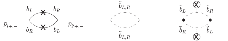
FIG. 1.: One-loop diagrams giving rise to a mass splitting between the states $\tilde{\nu}_{i,+}$ and $\tilde{\nu}_{i^{\prime},-}$, with $i,i^{\prime}=1,2,3$. The first two diagrams are $\lambda^{\prime}$-induced, the third one, $A^{\prime}$-induced.

All these diagrams are quadratically divergent. Once the infinities are removed through a renormalization procedure, the finite parts, evaluated at the sneutrino scale itself, taken here to be $m_{\tilde{L}}^{2}$, provide corrections to the elements of the sneutrino mass matrix. For states with definite CP $\sigma$ ($\sigma=+1,-1$), these become

$$m^{2}_{\tilde{\nu}_{ii^{\prime},\sigma}}=m^{2}_{\tilde{L}}\delta_{ii^{\prime}}+\epsilon^{2}_{ii^{\prime},\sigma}\,.$$ (12)

These corrections are, in general, different for states with different $\sigma$. Indeed, the sneutrino interactions involved in the diagrams of Fig. 1 are different for sneutrino states with different $\sigma$, as an inspection of the Lagrangian terms listed in Appendix A shows. Notice that no splitting is obtained from tadpole diagrams with virtual exchange of $\tilde{b}$ and $\tilde{\tau}$ states. This is because the quartic scalar interactions inducing these diagrams, $\tilde{f}_{L}^{\ast}\tilde{f}_{L}\tilde{\nu}_{i}^{\ast}\tilde{\nu}_{i}$ and $\tilde{f}_{R}^{\ast}\tilde{f}_{R}\tilde{\nu}_{i}^{\ast}\tilde{\nu}_{i}$ ($f=b,\tau$), are equal for sneutrino states with different CP. Thus, the finite parts of the tadpole diagrams give rise to small shifts in the sneutrino mass terms that are identical for states with different CP and, therefore, irrelevant for our discussion. In the following analysis, we neglect them altogether.

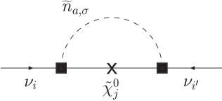
FIG. 2.: Contribution to the Majorana neutrino mass due to one-loop corrected states $\tilde{n}_{a,\sigma}$. The couplings $\tilde{\chi}_{j}^{0}-\nu_{i}-\tilde{n}_{a,\sigma}$ indicated here by a square, are given explicitly in Appendix A.

Once a splitting in mass for sneutrino states with different CP is generated, the one-loop diagram with neutralino-sneutrino exchange, shown in Fig. 2, can produce nonvanishing contributions to neutrino masses. In this case, however, since the sneutrino mass splitting terms are induced at the one loop, this is in reality a diagram arising at the two-loop level. We postpone this discussion to a later point of this paper and we proceed to the calculation of the diagram in Fig. 2, where the neutrino-sneutrino-neutralino vertices are one-loop corrected. As Appendix A shows, this simply means that these vertices are now weighted by the elements of the orthogonal rotation matrices needed to obtain the sneutrino mass eigenstates from the current eigenstates $\tilde{\nu}_{i,\sigma}$. We denote the sneutrino mass eigenstates by the symbol $\tilde{n}_{a,\sigma}$ ($a=1,2,3$) and the two rotation matrices by $O^{\sigma}$:

$$\tilde{\nu}_{i,\sigma}\ =\ \sum_{a}O_{ia}^{\,\sigma}\,\tilde{n}_{a,\sigma}\,.$$ (13)

These two matrices are determined by the one-loop corrections $\epsilon_{ii^{\prime},\sigma}^{2}$. Because of the assumption in Eq. (11), the new states $\tilde{n}_{a,\sigma}$ have mass:

$$m^{2}_{\tilde{n}_{a,\sigma}}\ =\ \sum_{k,k^{\prime}}O_{ka}^{\,\sigma}m^{2}_{\tilde{\nu}_{kk^{\prime},\sigma}}O_{k^{\prime}a}^{\,\sigma}\ =\ m^{2}_{\tilde{L}}+\sum_{k,k^{\prime}}O_{ka}^{\,\sigma}\epsilon^{2}_{kk^{\prime},\sigma}O_{k^{\prime}a}^{\,\sigma}\,.$$ (14)

For the calculation of the diagram in Fig. 2, the momentum dependence in the loop-corrected part of the sneutrino mass terms must be reinstated back explicitly. For neutrino mass terms evaluated at vanishing momentum square, we obtain

$$m_{\nu_{ii^{\prime}}}=i\,\frac{g^{2}}{4}\sum_{j,a}\left(\delta_{j\tilde{W}}+\delta_{j\tilde{B}}\tan^{2}\theta_{W}\right)\int\frac{d^{4}p}{(2\pi)^{4}}\frac{m_{\tilde{\chi}^{0}_{j}}}{p^{2}-m_{\tilde{\chi}^{0}_{j}}^{2}}\left\{\frac{O^{+}_{ia}O^{+}_{i^{\prime}a}(p^{2})}{p^{2}-m^{2}_{\tilde{n}_{a,+}}(p^{2})}-\frac{O^{-}_{ia}O^{-}_{i^{\prime}a}(p^{2})}{p^{2}-m^{2}_{\tilde{n}_{a,-}}(p^{2})}\right\}\,,$$ (15)

where $g$ is the weak coupling constant, $\theta_{W}$ the electroweak mixing angle, and the sum over $j$ extends to the two gaugino-like neutralinos. These are assumed to be nearly pure gauginos, so that the neutralino diagonalization matrix reduces to the unity matrix. An expansion of each term in the curly bracket in powers of the corresponding $\epsilon^{2}_{ii^{\prime},\sigma}$, gives

$$\sum_{a}\frac{O^{\sigma}_{ia}O^{\sigma}_{i^{\prime}a}(p^{2})}{p^{2}-m^{2}_{\tilde{n}_{a,\sigma}}(p^{2})}=\frac{\delta_{ii^{\prime}}}{p^{2}-m^{2}_{\tilde{L}}}+\frac{\epsilon^{2}_{ii^{\prime},\sigma}(p^{2})}{(p^{2}-m^{2}_{\tilde{L}})^{2}}+...\,,$$ (16)

with the ellipsis denoting higher order terms in $\epsilon^{2}_{ii^{\prime},\sigma}$. Thus, Eq. (15) reduces to

$$m_{\nu_{ii^{\prime}}}=i\,\frac{g^{2}}{4}\sum_{j}\left(\delta_{j\tilde{W}}+\delta_{j\tilde{B}}\tan^{2}\theta_{W}\right)m_{\tilde{\chi}^{0}_{j}}\int\frac{d^{4}p}{(2\pi)^{4}}\frac{\delta m^{2}_{\tilde{\nu}_{i,i^{\prime}}}(p^{2})}{(p^{2}-m_{\tilde{\chi}^{0}_{j}}^{2})(p^{2}-m_{\tilde{L}}^{2})^{2}}\,,$$ (17)

where the quantities $\delta m^{2}_{\tilde{\nu}_{i,i^{\prime}}}(p^{2})$, defined as

$$\delta m^{2}_{\tilde{\nu}_{i,i^{\prime}}}(p^{2})\ \equiv\ \epsilon^{2}_{ii^{\prime},+}(p^{2})-\epsilon^{2}_{ii^{\prime},-}(p^{2})\,,$$ (18)

are nothing but the splitting in the mass of the CP-even and CP-odd $ii^{\prime}$ sneutrino states, at the current eigenstate level.

A calculation of the diagrams in Fig. 1, yields results for these sneutrino mass splitting terms that can be expressed, in all generality, in terms of $B$ functions (see Appendix B). To show more explicitly their dependence on supersymmetric parameters, we give here approximated expressions, obtained in the limit $p^{2}=0$, separately for the $\lambda^{\prime}$- and the $A^{\prime}$-induced terms:

$$\left(\delta m^{2}_{\tilde{\nu}_{i,i^{\prime}}}(0)\right)|_{\lambda^{\prime}} = \frac{3}{4\pi^{2}}\,\lambda^{\prime}_{i33}\lambda^{\prime}_{i^{\prime}33}\,m^{2}_{b}\ \ln\left(\frac{m^{2}_{\tilde{b}_{2}}m^{2}_{\tilde{b}_{1}}}{m_{b}^{4}}\right)\,,$$ (19)

$$\left(\delta m^{2}_{\tilde{\nu}_{i,i^{\prime}}}(0)\right)|_{A^{\prime}} = \frac{3}{4\pi^{2}}\,A^{\prime}_{i33}A^{\prime}_{i^{\prime}33}\,\left(m^{2}_{\tilde{b},LR}\right)^{2}S(m^{2}_{\tilde{b}_{1}},m^{2}_{\tilde{b}_{2}})\,.$$ (20)

The first contribution has a mild logarithmic dependence on sfermion masses; the second, has a power dependence on them. The function $S(m^{2}_{\tilde{b}_{1}},m^{2}_{\tilde{b}_{2}})$ is defined in Appendix C and has the limiting value $-1/(6m^{4}_{\tilde{b}})$ for $m_{\tilde{b}_{1}}\to m_{\tilde{b}_{2}}\equiv m_{\tilde{b}}$. Similar contributions are obtained from diagrams with $\tau-\tilde{\tau}$ exchange, induced by the couplings $\lambda_{i33}$ and $A_{i33}$. The results for these diagrams can be read off those in Eqs. (19) and (20), after removing the color factor $3$, and making the obvious replacements of couplings and masses. The overall sneutrino mass splitting is then given by the sum of the two contributions in Eqs. (19) and (20), plus the two contributions coming from diagrams with $\tau-\tilde{\tau}$ exchange.

It is interesting to notice that the parameters $m^{2}_{\tilde{b},LR}$ and $\lambda^{\prime}_{i33}\lambda^{\prime}_{i^{\prime}33}$ enter in two different contributions to the sneutrino mass splitting. The same holds for the parameters $m^{2}_{\tilde{\tau},LR}$ and $\lambda_{i33}\lambda_{i^{\prime}33}$. Therefore, a suppression of the one-loop contributions to neutrino masses through option (2), among those listed after Eq. (4), leaves $\left(\delta m^{2}_{\tilde{\nu}_{i,i^{\prime}}}(p^{2})\right)|_{\lambda^{\prime}}$ unaffected, whereas if option (1) is chosen, and $m^{2}_{\tilde{b},LR}$ or $m^{2}_{\tilde{\tau},LR}$ are relatively large, it is $\left(\delta m^{2}_{\tilde{\nu}_{i,i^{\prime}}}(p^{2})\right)|_{A^{\prime}}$ to remain unsuppressed. As for the size of these contributions to the sneutrino mass splitting, if we take the approximation $m_{\tilde{b}_{1}}\simeq m_{\tilde{b}_{2}}\equiv m_{\tilde{b}}$ and $m_{\tilde{\tau}_{1}}\simeq m_{\tilde{\tau}_{2}}\equiv m_{\tilde{\tau}}$, we get

$$\left(\frac{\left(\delta m^{2}_{\tilde{\nu}_{i,i^{\prime}}}(0)\right)|_{\lambda^{\prime}}}{m^{2}_{\tilde{L}}}\right) \simeq 1.3\times 10^{-3}\left(\lambda^{\prime}_{i33}\lambda^{\prime}_{i^{\prime}33}\right)\left[\frac{\ln(m_{\tilde{b}}/m_{b})}{\ln(100)}\right]\left(\frac{100\,{\rm GeV}}{m_{\tilde{L}}}\right)^{2}\,,$$ (21)

$$\left(\frac{\left(\delta m^{2}_{\tilde{\nu}_{i,i^{\prime}}}(0)\right)|_{\lambda}}{m^{2}_{\tilde{L}}}\right) \simeq 1.3\times 10^{-4}\left(\lambda_{i33}\lambda_{i^{\prime}33}\right)\left[\frac{\ln(m_{\tilde{\tau}}/m_{\tau})}{\ln(56)}\right]\left(\frac{100\,{\rm GeV}}{m_{\tilde{L}}}\right)^{2}\,,$$ (22)

for the $\lambda^{\prime}$ and $\lambda$ contributions, and

$$\left|\frac{\left(\delta m^{2}_{\tilde{\nu}_{i,i^{\prime}}}(0)\right)|_{A^{\prime}}}{m^{2}_{\tilde{L}}}\right| \simeq 1.3\times 10^{-6}\left(\frac{A^{\prime}_{i33}A^{\prime}_{i^{\prime}33}}{{\rm GeV}^{2}}\right)\left(\frac{m^{2}_{\tilde{b},LR}}{m^{2}_{\tilde{b}}}\right)^{2}\left(\frac{100\,{\rm GeV}}{m_{\tilde{L}}}\right)^{2}\,.$$ (23)

$$\left|\frac{\left(\delta m^{2}_{\tilde{\nu}_{i,i^{\prime}}}(0)\right)|_{A}}{m^{2}_{\tilde{L}}}\right| \simeq 4.2\times 10^{-7}\left(\frac{A_{i33}A_{i^{\prime}33}}{{\rm GeV}^{2}}\right)\left(\frac{m^{2}_{\tilde{\tau},LR}}{m^{2}_{\tilde{\tau}}}\right)^{2}\left(\frac{100\,{\rm GeV}}{m_{\tilde{L}}}\right)^{2}\,,$$ (24)

for the $A^{\prime}$ and $A$ contributions.

As we shall see, similar considerations hold for the neutrino mass terms obtained from Eq. (17), once the expression for the sneutrino mass splitting is substituted in, and the integral is performed. The exact analytic expression for $m_{\nu_{ii^{\prime}}}$ is cumbersome. We show here the expression obtained when $\delta m^{2}_{\tilde{\nu}_{i,i^{\prime}}}(p^{2})$ is approximated by $\delta m^{2}_{\tilde{\nu}_{i,i^{\prime}}}(0)$. The results obtained through this approximation are certainly not valid for evaluations in which factors of ${\cal O}(1)$ are important. They are, however, good enough for order of magnitude estimates. We get

$$m_{\nu_{ii^{\prime}}}\simeq\frac{g^{2}}{64\pi^{2}}\sum_{j}\left(\delta_{j\tilde{W}}+\delta_{j\tilde{B}}\tan^{2}\theta_{W}\right)m_{\tilde{L}}\left(\!\frac{\delta m^{2}_{\tilde{\nu}_{i,i^{\prime}}}(0)}{m_{\tilde{L}}^{2}}\!\right)J\left(m^{2}_{\tilde{\chi}^{0}_{j}},m^{2}_{\tilde{L}}\right)\,,$$ (25)

where $\delta m^{2}_{\tilde{\nu}_{i,i^{\prime}}}(0)$ is given by the sum of $\left(\delta m^{2}_{\tilde{\nu}_{i,i^{\prime}}}(0)\right)|_{\lambda^{\prime}}$ and $\left(\delta m^{2}_{\tilde{\nu}_{i,i^{\prime}}}(0)\right)|_{A^{\prime}}$ in Eqs. (19) and (20). The dimensionless function $J(m^{2}_{\tilde{\chi}^{0}_{j}},m^{2}_{\tilde{L}})$, defined explicitly in Appendix C, is positive definite and depends only on the ratio $y\equiv m^{2}_{\tilde{\chi}^{0}_{j}}/m^{2}_{\tilde{L}}$. Note that the critical proportionality to the neutralino mass, explicit in Eq. (17), is now hidden by the fact that a factor $m_{\tilde{\chi}^{0}_{j}}/m_{\tilde{L}}$ has been included in the function $J$. This is indeed the product of the ratio $m_{\tilde{\chi}^{0}_{j}}/m_{\tilde{L}}$ and the actual loop function $I^{\prime}(m^{2}_{1},m^{2}_{2})$, also given in Appendix C, and also depending only on the ratio $y$. The reason for this replacement is that the $J$ function is very slowly decreasing for $y\gtrsim 4.5$, where it reaches the maximum value $\simeq 0.57$. It is also very slowly decreasing from this point down to $y=1$, where it gets the value $1/2$. It has still the value $\sim 1/4$ at $y=0.1$, and it drops to $0$ as $\sqrt{y}$, for $y\to 0$.

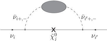
FIG. 3.: Two-loop contribution to Majorana neutrino mass terms. The grey oval indicates any of the one-loop diagrams in Fig. 1 generating a mass splitting for the sneutrino states $\tilde{\nu}_{i,+}$ and $\tilde{\nu}_{i^{\prime},-}$.

As preannounced, this contribution to neutrino mass is split in two terms. The first, as the one-loop contribution, depends on the product $\lambda^{\prime}_{i33}\lambda^{\prime}_{i^{\prime}33}$ ($\lambda_{i33}\lambda_{i^{\prime}33}$) but not on $m^{2}_{\tilde{b},LR}$ ($m^{2}_{\tilde{\tau},LR}$). Because of this, and because of the milder logarithmic dependence on scalar masses, it is less sensitive to the details of supersymmetry breaking than the one-loop neutrino-mass contribution. The second, on the contrary, is very sensitive to these details. It is directly proportional to $A^{\prime}_{i33}A^{\prime}_{i^{\prime}33}$ ($A_{i33}A_{i^{\prime}33}$), which do not have any influence on neutrino physics at the one-loop level.

The contribution to neutrino masses just calculated was treated as arising from one-loop diagrams with one-loop corrected vertices. That is to say, it is in reality a contribution originating at the two-loop level. The corresponding diagram is shown explicitly in Fig. 3, where the grey oval is any of the one-loop diagrams in Fig. 1. It is straightforward to see that the procedure followed here and the direct calculation of the two-loop diagram are completely equivalent and lead to the same Eq. (17).

Clearly, this equation does not exhaust all possible two-loop contributions to neutrino masses, neither all those proportional to the product of two $\lambda^{\prime}$ (or $\lambda$) couplings or of two $A^{\prime}$ (or $A$) couplings. Equation (17) encapsulates only the two-loop contributions that are induced by the one-loop generated splitting in the mass of CP-even and CP-odd sneutrino states . That is to say, the vertex corrections depicted by a black box in Fig. 2 are only due to the correction to the mass of the different sneutrino states.

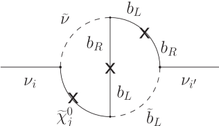
FIG. 4.: Another two-loop contribution to the Majorana neutrino mass.

Genuine vertex corrections for the interaction neutrino-sneutrino-neutralino, also due to $R_{p}$-violating couplings, would give rise to two-loop diagrams with a different topology. An example is explicitly shown in Fig. 4. The dependence on supersymmetric couplings in this diagram is as that of the diagram in Fig. 3, when the grey oval stands for the first diagram in Fig. 1. Such a diagram should not spoil our estimate of the constraints that neutrino masses induce on $R_{p}$-violating couplings. Other diagrams enter in the complete two-loop analysis, with the same topology as the diagram of Fig. 4. A complete calculation should, therefore, be performed.

IV Numerical Analysis

We are now in a position to discuss the numerical implications of our analysis. Equation (25) clearly bears what we claimed earlier, i.e. that the two-loop contributions to neutrino masses induced by the one-loop generated mass splitting between CP-even and CP-odd sneutrino states are quite large. This remains so, even after the one-loop contributions have been reduced as to avoid conflicts with experimental results.

First of all, the requirement that the neutrino mass terms do not exceed the $1\,$eV mark induces a constraint on the fractional splitting in the mass of CP-even and CP-odd sneutrino states that is independent from the $R_{p}$-violating couplings that have actually induced it. Taking the value $y=1$ for our numerical estimate, we obtain

$$\left(\!\frac{\delta m^{2}_{\tilde{\nu}_{i,i^{\prime}}}(0)}{m_{\tilde{L}}^{2}}\!\right)\ \lesssim\ 10^{-8}\left(\frac{100\,{\rm GeV}}{m_{\tilde{L}}}\right)\,.$$ (26)

This constraint is rather difficult to evade. For $m_{\tilde{L}}\simeq 100\,$GeV, a fractional splitting of a few GeV² would require $J(y)\sim\sqrt{y}\sim 10^{-4}$, resulting in $10\,$MeV weak-gaugino masses, which are already excluded by present experiments.

In turn, constraints on $R_{p}$-violating couplings can also be derived, namely,

$$\left(\lambda^{\prime}_{i33}\lambda^{\prime}_{i^{\prime}33}\right)\left[\frac{\ln(m_{\tilde{b}}/m_{b})}{\ln(100)}\right]\left(\frac{100\,{\rm GeV}}{m_{\tilde{L}}}\right) \lesssim 10^{-5}\,,$$ (27)

$$\left(\lambda_{i33}\lambda_{i^{\prime}33}\right)\left[\frac{\ln(m_{\tilde{\tau}}/m_{\tau})}{\ln(56)}\right]\left(\frac{100\,{\rm GeV}}{m_{\tilde{L}}}\right) \lesssim 10^{-4}\,,$$ (28)

for the $\lambda^{\prime}$- and $\lambda$-couplings, and

$$\left(A^{\prime}_{i33}A^{\prime}_{i^{\prime}33}\right)\left(\frac{m^{2}_{\tilde{b},LR}}{m^{2}_{\tilde{b}}}\right)^{2}\left(\frac{100\,{\rm GeV}}{m_{\tilde{L}}}\right) \lesssim 10^{-2}{\rm GeV}^{2}\,,$$ (29)

$$\left(A_{i33}A_{i^{\prime}33}\right)\left(\frac{m^{2}_{\tilde{\tau},LR}}{m^{2}_{\tilde{\tau}}}\right)^{2}\left(\frac{100\,{\rm GeV}}{m_{\tilde{L}}}\right) \lesssim 10^{-1}{\rm GeV}^{2}\,,$$ (30)

for the $A^{\prime}$- and $A$-couplings. Both sets of constraints depend only linearly on the sneutrino scale. Those on the products $\lambda^{\prime}_{i33}\lambda^{\prime}_{i^{\prime}33}$ and $\lambda_{i33}\lambda_{i^{\prime}33}$ have also a rather weak dependence on the sbottom and on the charged slepton scale, respectively.

If option (2) is chosen to suppress the one-loop contribution to the neutrino mass, i.e. if the left-right mixing terms in the sfermion mass matrices are very small, then Eq. (27) bounds the products $\lambda^{\prime}_{i33}\lambda^{\prime}_{i^{\prime}33}$ to be $\lesssim 10^{-5}$ for $m_{\tilde{b}}\sim 300\,$GeV and $m_{\tilde{L}}\sim 100\,$GeV. The products $A^{\prime}_{i33}A^{\prime}_{i^{\prime}33}$ remain unbounded. On the contrary, if the products of couplings $\lambda^{\prime}_{i33}\lambda^{\prime}_{i^{\prime}33}$ are constrained by the one-loop contributions to the neutrino mass terms, then only the products $A^{\prime}_{i33}A^{\prime}_{i^{\prime}33}$ are bounded by the two-loop analysis. They can be at most a few hundred GeV², if $m^{2}_{\tilde{b},LR}\sim m_{b}m_{\tilde{b}}$, $m_{\tilde{b}}\sim 300\,$GeV, and $m_{\tilde{L}}\sim 100\,$GeV. For $m^{2}_{\tilde{b},LR}\sim m^{2}_{\tilde{b}}$ and still $m_{\tilde{L}}\sim 100\,$GeV, the value of these products is reduced to $\sim 10^{-2}$ GeV².

Similar constraints hold for the product of couplings $\lambda_{i33}\lambda_{i^{\prime}33}$ and $A_{i33}A_{i^{\prime}33}$.

All the above discussion has been devoted to $R_{p}$-violating trilinear couplings with at least two third-generation indices. For couplings $\lambda^{\prime}_{ijk}$ and $A^{\prime}_{ijk}$ with $j=k\neq 3$, the analysis follows the same pattern as that for the case with $j=k=3$. The $b$-quark and the $\tilde{b}$-squarks must be replaced by the $d$- or $s$-quark and the $\tilde{d}$- or the $\tilde{s}$-squarks everywhere in the above equations. The constraints corresponding to those in Eq. (27) on $\lambda^{\prime}$-products with $j=k=2$ are about 3 or 4 order of magnitude weaker than those for $\lambda^{\prime}_{i33}\lambda^{\prime}_{i^{\prime}33}$, depending on the particular value used for the mass of the $s$-quark. They are completely lost for $j=k=1$. Therefore, if option (2) is chosen to reduce the one-loop contributions to neutrino masses, the products $A^{\prime}_{i22}A^{\prime}_{i^{\prime}22}$ and $A^{\prime}_{i11}A^{\prime}_{i^{\prime}11}$ as well as $\lambda^{\prime}_{i11}\lambda^{\prime}_{i^{\prime}11}$ remain substantially unsuppressed, whereas the bound $\lambda^{\prime}_{i22}\lambda^{\prime}_{i^{\prime}22}\lesssim 10^{-2}$ is obtained. In contrast, if option (1) is selected, the severity of both, the one-loop constraints on the $\lambda^{\prime}$-products and the two-loop ones on the $A^{\prime}$-products, depends on the mechanism of supersymmetry breaking. More precisely, it depends on whether the left-right mixing terms $m_{\tilde{f},LR}^{2}$ are proportional or not to the corresponding fermion mass $m_{f}$. In the former case, for a squark mass of $300\,$GeV, it is $\lambda^{\prime}_{i22}\lambda^{\prime}_{i^{\prime}22}\lesssim 10^{-3}-10^{-2}$, whereas $\lambda^{\prime}_{i11}\lambda^{\prime}_{i^{\prime}11}\sim{\cal O}(1)$ are still allowed. The two-loop constraints in Eq. (30) on the $A^{\prime}$-products would still easily allow couplings of type $A^{\prime}$ as large as $100\,$GeV or $\sim 1\,$TeV for $j=k=2$, and even larger for $j=k=1$. For $m_{\tilde{f},LR}^{2}$ independent from $m_{f}$, the results for the $A^{\prime}$ products are the same as in the case of $A^{\prime}_{i33}A^{\prime}_{i^{\prime}33}$, the constraints on the $\lambda^{\prime}$ products are: $\lambda^{\prime}_{i22}\lambda^{\prime}_{i^{\prime}22}\lesssim 10^{-7}-10^{-6}$ and $\lambda^{\prime}_{i11}\lambda^{\prime}_{i^{\prime}11}\lesssim 10^{-5}-10^{-4}$. As already mentioned, the uncertainties in the upper bounds discussed here is due to the uncertainty in the $s$- and $d$-quark masses.

Constraints on the products of $\lambda$ and $A$ couplings with indices $j=k=2$ or $j=k=1$ can be be obtained in a similar way.

	$m_{\tilde{f},LR}^{2}\lesssim 10^{-8}\,\left(\displaystyle{\frac{m_{b},m_{\tau}}{m_{f}}}\right)\,m^{2}_{\tilde{f}}$		$m_{\tilde{f},LR}^{2}=m_{f}\,m_{\tilde{f}}$		$m_{\tilde{f},LR}^{2}=m^{2}_{\tilde{f}}$
	1-loop	2-loop	1-loop	2-loop	1-loop	2-loop
$\lambda^{\prime}_{i33}\ (f\!=\!b)$	–	$10^{-2}$	$10^{-3}$	$10^{-2}$	$10^{-4}$	$10^{-2}$
$\lambda^{\prime}_{i22}\ (f\!=\!s)$	–	$10^{-1}$	$10^{-2}$	$10^{-1}$	$10^{-3}$	$10^{-1}$
$\lambda^{\prime}_{i11}\ (f\!=\!d)$	–	–	$\sim 1$	–	$10^{-3}$	–
$\lambda_{i33}\ (f\!=\!\tau)$	–	$10^{-2}$	$10^{-3}$	$10^{-2}$	$10^{-4}$	$10^{-2}$
$\lambda_{i22}\ (f\!=\!\mu)$	–	$10^{-1}$	$10^{-2}$	$10^{-1}$	$10^{-3}$	$10^{-1}$
$\lambda_{i11}\ (f\!=\!e)$	–	–	–	–	$10^{-2}$	–

TABLE I.: One- and two-loop upper limits on $\lambda^{\prime}_{ijj}$ and $\lambda_{ijj}$ ($i,j=1,2,3$) induced by the requirement that the neutrino mass terms do not exceed $1\,$eV. The numerical values used for quark and lepton masses are: $m_{b}=3\,$GeV, $m_{b}/m_{s}=40$, $m_{s}/m_{d}=20$, and $m_{\tau}=1.8\,$GeV, $m_{\tau}/m_{\mu}=20$, $m_{\mu}/m_{e}=200$. Squark masses are all fixed at $300\,$GeV, slepton and neutralino masses at $100\,$GeV. Different choices are made for $m^{2}_{\tilde{f},LR}$, from the very small to the rather large, see text. A horizontal bar indicates that the corresponding $\lambda^{\prime}_{ijj}$ or $\lambda_{ijj}$ are allowed to be even larger than 1.

A summary of the upper bounds for each of the $R_{p}$-violating couplings discussed so far is given in Table I and II. In particular, Table I lists the upper limits for the couplings $\lambda^{\prime}_{ijj}$ and $\lambda_{ijj}$, Table II, those for the couplings $A^{\prime}_{ijj}$ and $A_{ijj}$. For the numerical calculation, the values $m_{b}=3\,$GeV, $m_{b}/m_{s}=40$, $m_{s}/m_{d}=20$ were used for the quark masses, $m_{\tau}=1.8\,$GeV, $m_{\tau}/m_{\mu}=20$, and $m_{\mu}/m_{e}=200$, for the lepton masses. The squark masses were fixed as: $m_{{\tilde{d}}_{1,2}}=m_{{\tilde{s}}_{1,2}}=m_{{\tilde{b}}_{1,2}}=m_{\tilde{q}}=300\,$GeV. Finally, $m_{{\tilde{e}}_{1,2}}=m_{\tilde{\mu}_{1,2}}=m_{\tilde{\tau}_{1,2}}=m_{\tilde{\ell}}=100\,$GeV, and $m_{\tilde{L}}=m_{\tilde{W}}=100\,$GeV were chosen for the sleptons and the neutralino masses. In both tables the constraints are given for different possible values of $m^{2}_{\tilde{f},LR}$: $m_{\tilde{f},LR}^{2}\lesssim 10^{-8}\,(m_{b}/m_{f})\,m^{2}_{\tilde{f}}$, which sufficiently suppresses the one-loop contribution to neutrino masses; $m_{\tilde{f},LR}^{2}=m_{f}\,m_{\tilde{f}}$; and $m_{\tilde{f},LR}^{2}=m^{2}_{\tilde{f}}$. Note that the 2-loop constraints on $\lambda$ and $\lambda^{\prime}$ couplings do not depend on $m^{2}_{\tilde{f},LR}$, see Eq. (19), and therefore are important only when option (2) is chosen to suppress the one-loop contribution to neutrino mass, i.e. for $m_{\tilde{f},LR}^{2}\lesssim 10^{-8}m_{\tilde{f}}^{2}$. The constraints on $A$ and $A^{\prime}$ couplings do not depend on $m_{f}$, but they depend on $m_{\tilde{f},LR}^{2}$. For $m_{\tilde{f},LR}^{2}=m^{2}_{\tilde{f}}$, they are completely flavor independent, see Eq. (20). A horizontal bar in both tables indicates that the corresponding coupling is completely unconstrained. That is to say, even values larger than 1, in the case of $\lambda^{\prime}_{ijj}$ or $\lambda_{ijj}$, and larger than $1\,$TeV, in the case of $A^{\prime}_{ijj}$ or $A_{ijj}$ are not in conflict with the required smallness of neutrino masses.

	$m_{\tilde{f},LR}^{2}\lesssim 10^{-8}\,\left(\displaystyle{\frac{m_{b},m_{\tau}}{m_{f}}}\right)\,m^{2}_{\tilde{f}}$	$m_{\tilde{f},LR}^{2}=m_{f}\,m_{\tilde{f}}$	$m_{\tilde{f},LR}^{2}=m^{2}_{\tilde{f}}$
$A^{\prime}_{i33}\ (f\!=\!b)$	–	$10\,$GeV	$0.1\,$GeV
$A^{\prime}_{i22}\ (f\!=\!s)$	–	$\sim\!1\,$TeV	$0.1\,$GeV
$A^{\prime}_{i11}\ (f\!=\!d)$	–	–	$0.1\,$GeV
$A_{i33}\ (f\!=\!\tau)$	–	$10\,$GeV	$0.1\,$GeV
$A_{i22}\ (f\!=\!\mu)$	–	$100\,$GeV	$0.1\,$GeV
$A_{i11}\ (f\!=\!e)$	–	–	$0.1\,$GeV

TABLE II.: Same as in Table I, for the couplings $A^{\prime}_{ijj}$ and $A_{ijj}$ with $i,j=1-3$. These constraints are obtained at the two-loop level. A horizontal bar indicates that the corresponding $A^{\prime}_{ijj}$ or $A_{ijj}$ are allowed to be even larger than $1\,$TeV.

Note that an overall increase by a factor of $3$ in all sfermion masses, i.e. $m_{\tilde{q}}\sim 1\,$TeV and $m_{\tilde{\ell}}=m_{\tilde{L}}=300\,$GeV, would affect the constraints on the products of $R_{p}$-violating couplings, but it would not change the upper bounds on the $\lambda^{\prime}$ and $A^{\prime}$ couplings. It can, however, weaken those for $\lambda_{i22}$, $A_{i33}$, and $A_{i22}$ by one order of magnitude, when $m_{\tilde{f},LR}^{2}=m_{f}\,m_{\tilde{f}}$.

The situation is more complicated for couplings in which only one index $j$ or $k$ is $3$, while the other is not. The constraints on the different products of couplings cannot be simply gleaned from the results presented here and require an independent calculation. Not all diagrams in Fig. 1, for example, contribute to the sneutrino mass splitting and the interaction terms are more involved than those presented in Appendix A. Such a calculation goes beyond the scope of this paper and calls for an independent analysis. We can only guess that the constraints in these cases are less severe than in the case $j=k=3$, but probably more bounding than those obtained in the cases $j=k=2$ and $j=k=1$.

We would like to stress again that the constraints just derived are up to coefficients of ${\cal O}(1)$. The use of Eq. (17), instead of Eq. (25), gives rise to small imaginary parts for the neutrino mass terms. They are due to the analytic cuts that the loop functions for the diagrams in Fig. 1 have at large $p^{2}$. These aspects of the exact calculation, although interesting, are inconsequential for our discussion. We have explicitly checked that the order of magnitude of our estimates is, indeed, quite reliable.

V Conclusions

We conclude this paper with the following observations. The smallness of neutrino mass is, indeed, one of the most powerful constraints on some of the $R_{p}$-violating couplings involving third-generation indices. Contrary to what may be naively thought, the two-loop contributions to neutrino masses are very important to constrain such couplings. Barring cancellations in which the phases of these couplings play an important role, the complete one- and two-loop analysis indicates that it is rather unlikely that the couplings $\lambda^{\prime}_{i33}$ and $\lambda_{i33}$ are above the percent level. Such a constraint, obtained from two-loop contributions to neutrino masses, is irrespective of the value of the left-right mixing terms in the sbottom and stau mass matrices. It can only become more severe if these mixing terms are nonnegligible and the one-loop contributions to neutrino masses are unsuppressed. On the contrary, the soft trilinear parameters $A^{\prime}_{i33}$ and $A_{i33}$, which enter only in two-loop contributions to neutrino masses, are rather weakly constrained. The most stringent upper bound, obtained for very large left-right mixing terms, is only $0.1\,$GeV. They are completely unbounded from above for small left-right mixing terms.

Some of the consequences that the constraints derived here have for collider physics are discussed in Ref. [10].

Acknowledgements The authors acknowledge the financial support of the Japanese Society for Promotion of Science.

A Interaction terms

In this Appendix are listed the interaction Lagrangian terms needed for the calculations presented in the text. In the limit in which the two lightest neutralinos are pure gauginos, the neutralino-sneutrino-neutrino interactions terms are

$${\cal L}_{\rm tree} \supset -\frac{g}{\sqrt{2}}\sum_{i,j}\left(\delta_{j\tilde{W}}-\delta_{j\tilde{B}}\tan\theta_{W}\right)\left\{\overline{(\tilde{\chi}_{j}^{0})}P_{L}\nu_{i}\,\tilde{\nu}_{i}^{\ast}+\overline{\nu_{i}}P_{R}\tilde{\chi}_{j}^{0}\,\tilde{\nu}_{i}\right\}$$ (A1)

$$= -\,\frac{g}{2}\,\sum_{i,j}\left(\delta_{j\tilde{W}}-\delta_{j\tilde{B}}\tan\theta_{W}\right)\,\left\{\overline{(\tilde{\chi}_{j}^{0})}\nu_{i}\tilde{\nu}_{i,+}+i\overline{(\tilde{\chi}_{j}^{0})}\gamma_{5}\nu_{i}\tilde{\nu}_{i,-}\right\}\,,$$ (A2)

where the fact that both neutrinos and neutralinos are Majorana particles was used. Once one-loop corrections to the sneutrino sector are included, the neutralino-sneutrino-neutrino interactions terms can be expressed in terms of the mass eigenstates $\tilde{n}_{a\sigma}$ ($\sigma=+1,-1$), defined in Eq. (13), as

$${\cal L}_{{\rm 1-loop}|\tilde{\nu}}\ \supset\ -\frac{g}{2}\sum_{i,j,a}\left(\delta_{j\tilde{W}}-\delta_{j\tilde{B}}\tan\theta_{W}\right)\left\{O^{+}_{ia}\overline{(\tilde{\chi}_{j}^{0})}\nu_{i}\tilde{n}_{a,+}+iO^{-}_{ia}\overline{(\tilde{\chi}_{j}^{0})}\gamma_{5}\nu_{i}\tilde{n}_{a,-}\right\}\,.$$ (A3)

At the tree level, the current eigenstates $\tilde{\nu}_{i\sigma}$ and the mass eigenstates $\tilde{n}_{a\sigma}$ coincide.

The $R_{p}$-violating terms obtained from the superpotential in Eq. (1) are

$${\cal L}_{\rm tree} \supset -\sum_{i}\left\{\lambda_{i33}^{\prime}\,\left(\overline{b_{R}}\,b_{L}\right)\tilde{\nu}_{i}+\lambda_{i33}\,\left(\overline{\tau_{R}}\,\tau_{L}\right)\tilde{\nu}_{i}\right\}+{\rm H.c.}$$ (A4)

$$= -\sum_{i}\left\{\frac{\lambda_{i33}^{\prime}}{\sqrt{2}}\left[\bar{b}b\,\tilde{\nu}_{i,+}-i\,\bar{b}\gamma_{5}b\,\tilde{\nu}_{i,-}\right]+\frac{\lambda_{i33}}{\sqrt{2}}\left[\bar{\tau}\tau\,\tilde{\nu}_{i,+}-i\,\bar{\tau}\gamma_{5}\tau\,\tilde{\nu}_{i,-}\right]\right\}\,.$$ (A5)

Note that both sets of couplings $\lambda^{\prime}_{i33}$ and $\lambda_{i33}$ are taken to be real. In other words, of the three options listed in the text after Eq. (4), option (3) is not considered likely to be the one suppressing the one-loop contributions to neutrino masses.

The sneutrino-sbottom-sbottom interaction terms and the sneutrino-stau-stau ones, respectively proportional to the $\lambda^{\prime}$ and $\lambda$ couplings, and coming from $F$-terms, are

$${\cal L}_{\rm tree} \supset -\sum_{i}\left\{m_{b}\lambda_{i33}^{\prime}\left(\tilde{b}^{\ast}_{R}\tilde{b}_{R}+\tilde{b}^{\ast}_{L}\tilde{b}_{L}\right)\tilde{\nu}_{i}+m_{\tau}\lambda_{i33}\left(\tilde{\tau}^{\ast}_{R}\tilde{\tau}_{R}+\tilde{\tau}^{\ast}_{L}\tilde{\tau}_{L}\right)\tilde{\nu}_{i}\right\}+{\rm H.c.}$$ (A6)

$$= -{\sqrt{2}}\sum_{i,j}\left\{m_{b}\lambda_{i33}^{\prime}\left(\tilde{b}^{\ast}_{j}\tilde{b}_{j}\right)\tilde{\nu}_{i,+}+m_{\tau}\lambda_{i33}\left(\tilde{\tau}^{\ast}_{j}\tilde{\tau}_{j}\right)\tilde{\nu}_{i,+}\right\}\,.$$ (A7)

Again, the assumption of real $\lambda_{i33}^{\prime}$ and $\lambda_{i33}$ couplings was made. Notice that no interaction terms for the CP-odd states is generated by $F$-term contributions to the Lagrangian.

Finally, contributions to the sneutrino-sbottom-sbottom interaction terms and to the sneutrino-stau-stau ones, come also from the scalar potential in Eq. (2). They are

$${\cal L}_{\rm tree}\ \supset\ -\sum_{i}\left\{A^{\prime}_{i33}\tilde{b}_{L}^{\ast}\tilde{b}_{R}\tilde{\nu}_{i}+A_{i33}\tilde{\tau}_{L}^{\ast}\tilde{\tau}_{R}\tilde{\nu}_{i}\right\}+{\rm H.c.}\,.$$ (A8)

Once the $2\times 2$ sbottom mass squared matrix is diagonalized, the first term becomes

$${\cal L}_{\rm tree}=-\sum_{i}\frac{A^{\prime}_{i33}}{\sqrt{2}}\left\{\left[\sin 2\theta_{\tilde{b}}\left(\tilde{b}_{1}^{\ast}\tilde{b}_{1}-\tilde{b}_{2}^{\ast}\tilde{b}_{2}\right)+\cos 2\theta_{\tilde{b}}\left(\tilde{b}_{1}^{\ast}\tilde{b}_{2}+\tilde{b}_{2}^{\ast}\tilde{b}_{1}\right)\right]\tilde{\nu}_{i,+}+i\left[\tilde{b}_{2}^{\ast}\tilde{b}_{1}-\tilde{b}_{1}^{\ast}\tilde{b}_{2}\right]\tilde{\nu}_{i,-}\right\}\,,$$ (A9)

where $\theta_{\tilde{b}}$ is the diagonalization angle of the $2\times 2$ sbottom mass squared matrix. A similar expression is obtained for the sneutrino-stau-stau interaction term in Eq. (A8).

Note that, for the purpose of obtaining neutrino mass terms induced by the splitting in mass for the CP-even and CP-odd sneutrino states, it is sufficient to consider the effect of sneutrino mass corrections on the neutralino-sneutrino-neutrino interaction terms only. The inclusion of such corrections to the other interaction terms in Eqs. (A5), (A7), and (A9) is irrelevant for the calculation of neutrino mass terms induced by a nonvanishing splitting in the mass of CP-even and CP-odd sneutrino states.

B Sneutrino mass-splitting terms

We list here the formulae obtained for the sneutrino mass splitting from one-loop diagrams:

$$(\delta m_{\tilde{\nu}_{ii^{\prime}}}^{2}(p^{2}))^{(1)}|_{A^{\prime}} = -\frac{3}{4\pi^{2}}A^{\prime}_{i33}A^{\prime}_{i^{\prime}33}\left(\frac{m^{2}_{\tilde{b},LR}}{m^{2}_{\tilde{b}_{2}}-m^{2}_{\tilde{b}_{1}}}\right)^{2}\times$$ (B2)

$$\left(B_{0}(p^{2},m^{2}_{\tilde{b}_{1}},m^{2}_{\tilde{b}_{1}})+B_{0}(p^{2},m^{2}_{\tilde{b}_{2}},m^{2}_{\tilde{b}_{2}})-2B_{0}(p^{2},m^{2}_{\tilde{b}_{1}},m^{2}_{\tilde{b}_{2}})\right)\,,$$

$$(\delta m_{\tilde{\nu}_{ii^{\prime}}}^{2}(p^{2}))^{(1)}|_{\lambda^{\prime}} = -\frac{3}{4\pi^{2}}\lambda^{\prime}_{i33}\lambda^{\prime}_{i^{\prime}33}\,m_{b}^{2}\times$$ (B4)

$$\left(B_{0}(p^{2},m^{2}_{\tilde{b}_{1}},m^{2}_{\tilde{b}_{1}})+B_{0}(p^{2},m^{2}_{\tilde{b}_{2}},m^{2}_{\tilde{b}_{2}})-2B_{0}(p^{2},m^{2}_{b},m^{2}_{b})\right)\,,$$

where the function $B_{0}(p^{2},m_{1}^{2},m^{2}_{2})$ is defined as [20]:

$$B_{0}(p^{2},m_{1}^{2},m^{2}_{2})=\int\frac{\overline{d^{D}k}}{i\pi^{2}}\frac{1}{(k^{2}-m_{1}^{2}+i\epsilon)[(k+p)^{2}-m_{2}^{2}+i\epsilon]}\,,$$ (B5)

where $D=4-2\,\epsilon$ and $\overline{d^{D}k}=\Gamma(1-\epsilon)(\pi\mu^{2})^{\epsilon}d^{D}k$.

C Loop functions

We list here the functions arising from loop integrations:

$$I(m_{1}^{2},m_{2}^{2},0) = \frac{\ln(m_{2}^{2})-\ln(m_{1}^{2})}{m_{2}^{2}-m_{1}^{2}}\,,$$ (C1)

$$S(m^{2}_{1},m^{2}_{2}) = \frac{2}{(m^{2}_{2}-m^{2}_{1})^{3}}\left(m^{2}_{2}-m^{2}_{1}+\frac{m^{2}_{2}+m^{2}_{1}}{2}\ln\left(\frac{m^{2}_{1}}{m^{2}_{2}}\right)\right)\,,$$ (C2)

$$I^{\prime}(m^{2}_{1},m^{2}_{2}) = \frac{1-y+y\ln{y}}{\left(1-y\right)^{2}}\,,\quad\quad y\equiv\left(\frac{m^{2}_{1}}{m^{2}_{2}}\right)\,.$$ (C3)

They are respectively the functions obtained from the fermion-sfermion loop giving rise to the one-loop neutrino mass contribution; from the sfermion-sfermion contribution giving rise to the one-loop correction to sneutrino masses proportional to the $A^{\prime}$ and $A$ soft parameters; and from the sneutrino-neutralino loop giving rise to neutrino mass terms.

The function $J(m_{1}^{2},m_{2}^{2})$ also used in the text is

$$J(m_{1}^{2},m_{2}^{2})=\sqrt{\frac{m_{1}^{2}}{m_{2}^{2}}}\,I^{\prime}(m^{2}_{1},m^{2}_{2})\,.$$ (C4)

REFERENCES

• [1] G. R. Farrar and P. Fayet, Phys. Lett. B 76 (1978) 575;
C. S. Aulakh and R. N. Mohapatra, Phys. Lett. B 119 (1982) 136;
F. Zwirner, Phys. Lett. B 132 (1983) 103;
L. J. Hall and M. Suzuki, Nucl. Phys. B 231 (1984) 419;
I. H. Lee, Nucl. Phys. B 246 (1984) 120;
J. R. Ellis, G. Gelmini, C. Jarlskog, G. G. Ross and J. W. Valle, Phys. Lett. B 150 (1985) 142;
G. G. Ross and J. W. Valle, Phys. Lett. B 151 (1985) 375;
S. Dawson, Nucl. Phys. B 261 (1985) 297;
R. Barbieri and A. Masiero, Nucl. Phys. B 267 (1986) 679;
S. Dimopoulos and L. J. Hall, Phys. Lett. B 207 (1988) 210.
• [2] For reviews, see, for example: G. Bhattacharyya, Nucl. Phys. Proc. Suppl.  52A (1997) 83;
H. K. Dreiner, arXiv:hep-ph/9707435;
G. Bhattacharyya, arXiv:hep-ph/9709395;
R. Barbier et al., arXiv:hep-ph/9810232;
O. C. Kong, Nucl. Phys. Proc. Suppl.  101 (2001) 421.
• [3] L. E. Ibanez and G. G. Ross, Nucl. Phys. B368 (1992) 3.
• [4] J. Erler, J. L. Feng and N. Polonsky, Phys. Rev. Lett.  78 (1997) 3063.
• [5] F. Borzumati, J. Kneur and N. Polonsky, Phys. Rev.  D60 (1999) 115011.
• [6] S. Bar-Shalom, G. Eilam and A. Soni, Phys. Rev. Lett.  80 (1998) 4629;
S. Bar-Shalom, G. Eilam, J. Wudka and A. Soni, Phys. Rev. D 59 (1999) 035010.
• [7] M. Chaichian, K. Huitu and Z. H. Yu, Phys. Lett. B 508 (2001) 317;
M. Chaichian, K. Huitu, S. Roy and Z. H. Yu, Phys. Lett. B 518 (2001) 261.
• [8] S. Roy and B. Mukhopadhyaya, Phys. Rev. D 55 (1997) 7020;
B. Mukhopadhyaya, S. Roy and F. Vissani, Phys. Lett. B 443 (1998) 191;
E. J. Chun and J. S. Lee, Phys. Rev. D 60 (1999) 075006;
B. Mukhopadhyaya and S. Roy, Phys. Rev. D 60 (1999) 115012;
S. Y. Choi, E. J. Chun, S. K. Kang and J. S. Lee, Phys. Rev. D 60 (1999) 075002;
A. Datta, B. Mukhopadhyaya and F. Vissani, Phys. Lett. B 492 (2000) 324;
A. Bartl, W. Porod, D. Restrepo, J. Romao and J. W. Valle, Nucl. Phys. B 600 (2001) 39;
W. Porod, M. Hirsch, J. Romao and J. W. Valle, Phys. Rev. D 63 (2001) 115004;
V. D. Barger, T. Han, S. Hesselbach and D. Marfatia, Phys. Lett. B 538 (2002) 346;
E. J. Chun, D. W. Jung, S. K. Kang and J. D. Park, Phys. Rev. D 66 (2002) 073003.
• [9] F. Borzumati, R. M. Godbole, J. L. Kneur and F. Takayama, JHEP 0207 (2002) 037.
• [10] F. Borzumati, J. S. Lee and F. Takayama, arXiv:hep-ph/0206248.
• [11] L. J. Hall and M. Suzuki in [1];
A. Santamaria and J. W. Valle, Phys. Lett. B 195 (1987) 423;
J. C. Romao and J. W. Valle, Nucl. Phys. B 381 (1992) 87;
A. S. Joshipura and M. Nowakowski, Phys. Rev. D 51 (1995) 2421;
M. Nowakowski and A. Pilaftsis, Nucl. Phys. B 461 (1996) 19;
D. E. Kaplan and A. E. Nelson, JHEP 0001 (2000) 033;
F. Takayama and M. Yamaguchi, Phys. Lett. B 476 (2000) 116.
• [12] F. Borzumati, G. R. Farrar, N. Polonsky and S. Thomas, Nucl. Phys. B 555 (1999) 53.
• [13] J. M. Frere, M. V. Libanov and S. V. Troitsky, Phys. Lett. B 479 (2000) 343.
• [14] N. Polonsky, Lect. Notes Phys.  M68 (2001) 1 [arXiv:hep-ph/0108236].
• [15] S. Dimopoulos and L. J. Hall in [1];
K. S. Babu and R. N. Mohapatra, Phys. Rev. Lett.  64 (1990) 1705;
R. M. Godbole, P. Roy and X. Tata, Nucl. Phys. B 401 (1993) 67;
F. M. Borzumati, Y. Grossman, E. Nardi and Y. Nir, Phys. Lett. B 384 (1996) 123;
M. Drees, S. Pakvasa, X. Tata and T. ter Veldhuis, Phys. Rev. D 57, 5335 (1998);
S. Rakshit, G. Bhattacharyya and A. Raychaudhuri, Phys. Rev. D 59 (1999) 091701;
A. Abada and M. Losada, Nucl. Phys. B 585 (2000) 45;
A. Abada and M. Losada, Phys. Lett. B 492 (2000) 310;
Further references can be found in: A. Abada, S. Davidson and M. Losada, Phys. Rev. D 65 (2002) 075010.
• [16] Y. Grossman and H. E. Haber, Phys. Rev. Lett.  78 (1997) 3438.
• [17] E. J. Chun, Phys. Lett. B 525 (2002) 114;
K. Choi, K. Hwang and W. Y. Song, Phys. Rev. Lett.  88 (2002) 141801.
• [18] See, for example, Y. Grossman and H. E. Haber in [16];
S. Davidson and S. F. King, Phys. Lett. B 445 (1998) 191,
F. Borzumati and Y. Nomura, Phys. Rev. D 64 (2001) 053005;
N. Arkani-Hamed, L. J. Hall, H. Murayama, D. R. Smith and N. Weiner, Phys. Rev. D 64 (2001) 115011;
E. J. Chun, and K. Choi, K. Hwang and W. Y. Song in [17].
• [19] Y. Grossman and H. E. Haber, Phys. Rev. D 59 (1999) 093008 and Phys. Rev. D 63 (2001) 075011;
F. Borzumati, G. R. Farrar, N. Polonsky and S. Thomas in [12];
J. M. Frere, M. V. Libanov and S. V. Troitsky in [13].
• [20] See, for example, K. Hagiwara, S. Matsumoto, D. Haidt and C. S. Kim, Z. Phys. C 64, 559 (1994) [Erratum-ibid. C 68, 352 (1995)].