UH-511-1004-02 SLAC-PUB-9283 FSU-HEP-020709
Relating bottom quark mass in $\overline{\rm DR}$ and $\overline{\rm MS}$ regularization schemes

Abstract

The value of the bottom quark mass at $Q=M_{Z}$ in the $\overline{\rm DR}$ scheme is an important input for the analysis of supersymmetric models with a large value of $\tan\beta$. Conventionally, however, the running bottom quark mass extracted from experimental data is quoted in the $\overline{\rm MS}$ scheme at the scale $Q=m_{b}$. We describe a two loop procedure for the conversion of the bottom quark mass from $\overline{\rm MS}$ to $\overline{\rm DR}$ scheme. The Particle Data Group value $m_{b}^{\overline{\rm MS}}(m_{b}^{\overline{\rm MS}})=4.2\pm 0.2$ GeV corresponds to a range of 2.65–3.03 GeV for $m_{b}^{\overline{\rm DR}}(M_{Z})$.

I Introduction

Supersymmetry (SUSY) is one of the best-studied extensions of the Standard Model (SM) rev . Despite the lack of direct evidence, many theorists consider the idea promising enough to examine even quantum corrections in SUSY theories: these include corrections to SM quantities due to sparticle loops pierce , as well as corrections to processes involving the production and decays of supersymmetric particles zerwas . Quantum corrections in SUSY theories are also important for obtaining the implications of top-down models, where simple assumptions about symmetries of physics at the high scale result in a highly predictive scenario. The best known example of these is the correction carena to the relation between the down type mass and the corresponding superpotential Yukawa coupling, which is crucial to include when analysing SUSY models for large values of the parameter $\tan\beta$.

For large $\tan\beta$ values, third generation sparticle and Higgs boson masses as well as sparticle decay patterns, and thus collider signals for SUSY, are sensitive to the value of the bottom (and to a lesser extent tau) Yukawa coupling large . Knowledge of Yukawa couplings is also necessary for an analysis of the interesting possibility that these are unified at a high scale. Yukawa coupling unification may, for instance, be realized in the minimal $SO(10)$ SUSY model provided $\tan\beta$ is large soten . The interpretation of super-Kamiokande atmospheric neutrino data superk in terms of neutrino oscillations originating in a non-trivial flavour structure of the neutrino mass matrix has led to considerable recent interest us ; raby in such a scenario.

To include radiative corrections in the phenomenological analysis of supersymmetric models, the $\overline{\rm DR}$ regularization by dimensional reduction Siegel:1979wq , a modification of the conventional dimensional regularization is commonly used as a candidate for an invariant regularization of supersymmetric theories. Since the bottom quark Yukawa coupling is determined from the running bottom mass parameter at low energy, a careful determination of $m_{b}(M_{Z})$ in the $\overline{\rm DR}$ scheme is necessary.

On the other hand, it became a standard practice to use experimental data to extract the value of the running bottom mass parameter $m_{b}(m_{b})$ in the $\overline{\rm MS}$ renormalization scheme. The most recent results based on NNLO QCD analyses of the $\Upsilon$ sum rules can be found in  mass (see also the summary in  Groom:in which, however, also includes older (and by now obsolete) results in its world average). It is useful to explicitly examine what the allowed range of $m_{b}^{\overline{\rm MS}}(m_{b})$ note translates into when expressed in terms of $m_{b}^{\overline{\rm DR}}(M_{Z})$. While an immediate motivation to study this is because the allowed range of $m_{b}^{\overline{\rm DR}}(M_{Z})$ yields an estimate of the “error” within which Yukawa couplings in SUSY models with Yukawa coupling unification should be required to unify, our result for $m_{b}^{\overline{\rm DR}}(M_{Z})$ would be of relevance for any SUSY analysis with large $\tan\beta$.

Many authors aronson start with the value of the bottom quark mass $m_{b}^{\rm pole}$ to extract $m_{b}^{\overline{\rm DR}}(M_{Z})$, either by directly relating the pole mass to the running mass at the high scale (as described in Sec. II), or by first using the pole mass to derive $m_{b}^{\overline{\rm DR}}$ at the scale of the bottom quark mass and then evolving it to $M_{Z}$ using renormalization group equations. Since it became clear in recent years that the pole mass of the quark suffers from infra-red sensitivity which precludes its accurate determination from physical observables, this approach leads to significant ambiguities in the resulting value of $m_{b}^{\overline{\rm DR}}(M_{Z})$. In this paper, we suggest a better approach to the determination of $m_{b}^{\overline{\rm DR}}(M_{Z})$, which by-passes the use of the $b$-quark pole mass. The idea is to employ recent accurate determinations of $m_{b}(m_{b})$ in the $\overline{\rm MS}$ scheme mass , use the renormalization group running up to the scale $\mu=M_{Z}$ and use a relation between the $\overline{\rm MS}$ and $\overline{\rm DR}$ masses at that scale to obtain $m_{b}^{\overline{\rm DR}}(M_{Z})$. We will show that the relation that connects the masses in the two schemes at the same scale $\mu$ exhibits excellent convergence properties thereby making the suggested procedure very accurate and practically insensitive to higher order corrections.

II $\overline{\rm MS}$ and $\overline{\rm DR}$ mass formulas

Our final goal will be a relation between the $\overline{\rm MS}$ and $\overline{\rm DR}$ masses. However, since in the literature the two masses are usually related to the pole mass, we begin by collecting formulae that relate the pole mass of the bottom quark with its running mass (at any scale) in both the $\overline{\rm MS}$ and $\overline{\rm DR}$ schemes.

Currently, the relation between the $\overline{\rm MS}$ and pole quark mass is known through order ${\cal O}(\alpha_{s}^{3})$  Tarrach:1980up ; Gray:1990yh ; Fleischer:1998dw ; Chetyrkin:1999qi ; Chetyrkin:2000yt ; Melnikov:2000qh . In this paper we will only use the two loop relation between them:

$$\frac{m_{b}^{\overline{\rm MS}}(\mu)}{m_{b}^{\rm pole}}=1+a_{s}(\mu)\left(L-\frac{4}{3}\right)+a_{s}^{2}(\mu)\left(-\frac{11}{24}L^{2}\right.$$

$$\left.+\frac{197}{72}L-\frac{187}{32}+\frac{\zeta_{3}}{6}-\frac{\pi^{2}}{9}\ln 2-\frac{\pi^{2}}{9}-\Delta\right),$$ (1)

where $a_{s}(\mu)=\alpha_{s}(\mu)/\pi$ is the $\overline{\rm MS}$ coupling constant in the theory with five quark flavors, $L=\log(m_{b}^{2}(\mu)/\mu^{2})$, and $\Delta$ is a correction due to light quark mass effects (arising from the two-loop diagram with a second fermion-loop), given by Gray:1990yh ,

$$\Delta = \sum_{i=u,d,s,c}\delta\left(\frac{m_{i}}{m_{b}}\right)\;,$$ (2)

$$\delta(x) = \frac{\pi^{2}}{6}x(1+x^{2})-x^{2}+{\cal O}(x^{4}).$$ (3)

In the argument of $\Delta$ the ratio of quark masses of the light quarks to the bottom quark pole mass appear. For $0\leq x\leq 1$ the exact result is approximated by the three terms given in Eq. (3) within an accuracy of $1$%.

The relation between the pole mass and the quark running masses in the $\overline{\rm DR}$ renormalization scheme is known through ${\cal O}(\alpha_{s}^{2})$ Avdeev:1997sz . The result reads:

$$\frac{m_{b}^{\rm pole}}{m_{b}^{\overline{\rm DR}}(\mu)}=1+\bar{a}_{s}(\mu)\left(\frac{5}{3}-L_{1}\right)+\bar{a}_{s}^{2}(\mu)\left(\frac{35}{24}L_{1}^{2}\right.$$

$$\left.-\frac{395}{72}L_{1}+\frac{2159}{288}-\frac{\zeta_{3}}{6}+\frac{\pi^{2}}{9}+\frac{\pi^{2}}{9}\ln 2+\Delta\right),$$ (4)

where $\bar{a}_{s}(\mu)=\bar{\alpha}_{s}(\mu)/\pi$ is the strong coupling constant in the $\overline{\rm DR}$ scheme and $L_{1}=\ln(m_{b}^{\rm DR}(\mu)^{2}/\mu^{2})$.

It is possible to invert Eq. (1), expressing $m_{b}^{\rm pole}$ in terms of $m_{b}^{\overline{\rm MS}}(m_{b})$, and then use this together with Eq. (4) choosing $\mu=M_{Z}$ to obtain $m_{b}^{\overline{\rm DR}}(M_{Z})$. This is unsatisfactory for two reasons. First of all, the relation between $m_{b}^{\rm pole}$ and $m_{b}^{\overline{\rm DR}}(M_{Z})$ involves not so small logarithm ($C_{F}\bar{a}_{s}(M_{z})\log(M_{Z}^{2}/m^{2})\sim 0.3$) which leads to uncomfortably large corrections. Second, the perturbative corrections to the relation between $m_{b}^{\rm pole}$ and $m_{b}^{\overline{\rm MS}}(m_{b})$ are large. For example, including the ${\cal O}(\alpha_{s}^{3})$ term in Eq. (1) leads to a correction comparable to the contribution of the ${\cal O}(\alpha_{s}^{2})$ term. By the same token, when inverting Eq. (1) to determine the value of $m_{b}^{\rm pole}$ out of $m_{b}^{\overline{\rm MS}}$, it makes a significant numerical difference if one expands the inverse equation in powers of $a_{s}(\mu)$ or just keeps the r.h.s. of Eq. (1) in the denominator. These problems show that, as a consequence of large perturbative corrections, the final numerical results for $m_{b}^{\overline{\rm DR}}(M_{Z})$ when obtained from Eq. (1), are not stable against higher orders perturbative corrections. Analyses  aronson that use the pole mass as an input for extracting the short-distance mass, and via this, quark Yukawa couplings, will reflect this ambiguity. In what follows we suggest a procedure wherein the problems just mentioned are considerably ameliorated.

III $\overline{\rm DR}$ mass from the $\overline{\rm MS}$ bottom mass

The first of the above problems can be by-passed because an analytic solution of the renormalization group equation for the running mass in the $\overline{\rm MS}$ scheme is known. This was originally obtained at three loops  Tarasov:au and recently the four loop term has also been computed  Chetyrkin:1997dh . For the case of five active quark flavors, and up to NNLO renormalization group evolution, this takes the form

$$m_{b}^{\overline{\rm MS}}(\mu)= \hat{m}_{\rm MS}\left(\frac{23a_{s}(\mu)}{6}\right)^{12/23}\left(1+\frac{3731}{3174}~{}a_{s}(\mu)\right.$$ (5)

$$\left.+1.500706~{}a_{s}^{2}(\mu)\right)\;,$$

where the integration constant $\hat{m}_{\rm MS}$ is the renormalization group invariant bottom mass. We do not need to know $\hat{m}_{\rm MS}$ because, if we denote the right hand side as $\hat{m}_{\rm MS}F_{b}(\mu)$, the running mass at scale $M_{Z}$ can be calculated from a given running mass at scale $m_{b}(m_{b})$ using the expression,

$$m_{b}^{\overline{\rm MS}}(M_{Z})=m_{b}^{\overline{\rm MS}}(m_{b})\frac{F_{b}(M_{Z})}{F_{b}(m_{b})}$$ (6)

Although Eq. (5) has been written in the $\overline{\rm MS}$ scheme, we observe that the leading term, determined entirely by the first coefficient of the $\beta$-function $\beta_{0}$ and the first coefficient of the quark mass anomalous dimension $\gamma_{0}$, is scheme-independent. At $Q=M_{Z}$ the scheme-dependent subleading terms contribute $\sim 8$%. Most of this comes from the next to leading $\alpha_{s}/\pi$ term while the three loop term contributes just 0.2%. The coefficient of this two loop term can be readily evaluated in the $\overline{\rm DR}$ scheme using,

$$\gamma_{1}^{\overline{\rm DR}}=\gamma_{1}-\frac{\beta_{0}}{3}-\frac{\gamma_{0}}{4}\;,$$ (7)

where $\gamma_{1}$ is the coefficient of the ${\cal O}(\alpha_{s}^{2})$ term in the quark mass anomalous dimension. At two loops, we obtain for the running bottom mass in the $\overline{\rm DR}$ scheme,

$$m_{b}^{\overline{\rm DR}}(\mu)\equiv\hat{m}_{\rm DR}\left(\frac{23\bar{a}_{s}(\mu)}{6}\right)^{12/23}\left(1+\frac{753}{1058}~{}\bar{a}_{s}(\mu)\right)\;.$$ (8)

To compute the bottom running mass at $m_{b}$ we need the value of $\alpha_{s}(m_{b})$ that corresponds to the experimental measurement, $\alpha_{s}(M_{Z})$. To this end we will use the three loop analytical formula for $\alpha_{s}$  Tarasov:au in the $\overline{\rm MS}$ scheme, that is the solution of the corresponding Callan-Symanzyk equation. In the case of five active quark flavours the formula reduces to,

$$\alpha_{s}(\mu)=\frac{12\pi}{23t}\left[1-\frac{348}{529}\frac{\ln(t)}{t}\right.$$

$$\left.+\left(\frac{348}{529}\right)^{2}\frac{1}{t^{2}}\left(\left(\ln(t)-\frac{1}{2}\right)^{2}-\frac{78073}{242208}\right)\right],$$ (9)

where $t=\ln\left(\mu^{2}/\Lambda^{2}\right)$. In practice, it is convenient to use the value of $\alpha_{s}(M_{Z})$ to first determine $\Lambda$, and then use Eq. (9) again for the calculation of $\alpha_{s}(m_{b})$ which is inserted in Eq. (6) before the iteration. The four loop contributions to Eq. (9) have also been calculated  Vermaseren:1997fq and found to be small. It was observed that the previous three loop analytical solution for $\alpha_{s}(\mu)$ gives a very good aproximation to the numerical solution of the four loop RGE  Chetyrkin:1997sg . Finally, we note that to compute $\alpha_{s}(\mu)$ in the $\overline{\rm DR}$ scheme we convert $\alpha_{s}(\mu)_{\overline{\rm MS}}$ using  Antoniadis:1982vr ,

$$\frac{1}{\bar{a}_{s}(\mu)}=\frac{1}{a_{s}(\mu)}-\frac{1}{4}\;.$$ (10)

By eliminating the pole mass from the relations between the pole and running masses presented in the previous section, we can derive a two loop relation between the $\overline{\rm DR}$ and the $\overline{\rm MS}$ bottom masses at the same scale. ¿From (4) and (1), using Eq. (10) to convert the $\overline{\rm DR}$ coupling constant to the $\overline{\rm MS}$ coupling constant, we obtain:

$$m_{b}^{\overline{\rm DR}}(\mu)=m_{b}^{\overline{\rm MS}}(\mu)\left(1-\frac{1}{3}a_{s}(\mu)-\frac{29}{72}a_{s}(\mu)^{2}+{\cal O}(a_{s}^{3})\right).$$ (11)

This expression also appears, but is never used, in Ref. Avdeev:1997sz .

We were originally motivated to consider the relation between $\overline{\rm MS}$–$\overline{\rm DR}$ masses because it was clear that the leading logarithm corrections are absent because leading contributions to the QCD beta function and quark mass anomalous dimension are scheme-independent. The absence of all $\log\mu/m_{b}$ terms follows from the fact that both $\overline{\rm MS}$ and $\overline{\rm DR}$ are mass-independent renormalization schemes and that $(\gamma^{\overline{{\rm DR}}}-\gamma^{\overline{{\rm MS}}})/\beta^{\overline{{\rm MS}}}$ is regular around $\alpha_{s}=0$ note2 . The renormalization group equations then ensure that the relation between the two masses at the same scale can only depend on the coupling constant $\alpha_{s}(\mu)$.

The perturbative series in Eq. (11) exhibits excellent convergence of the perturbative expansion. This is to be expected, since the $\overline{\rm MS}$ and the $\overline{\rm DR}$ mass are both truly short-distance quantities. The infrared renormalon problem, which is the reason for large perturbative corrections in the relations between the pole mass of the quark and any of the short-distance masses, is not relevant there. Note that the cancellation of large corrections happens order by order in perturbation theory and for this reason one cannot improve on the obtained relation by including e.g. the three loop term from the relation between the pole and the $\overline{\rm MS}$ mass without including a similar term from the relation between the pole and the $\overline{\rm DR}$ mass.

These considerations suggest the following two step procedure for extracting $m_{b}^{\overline{\rm DR}}(M_{Z})$, starting from $m_{b}^{\overline{\rm MS}}(m_{b})$.

• First, evolve $m_{b}^{\overline{\rm MS}}(m_{b})$ to $Q=M_{Z}$ using (5) which is valid within the $\overline{\rm MS}$ scheme.

• Use Eq. (11) to convert $m_{b}^{\overline{\rm MS}}(M_{Z})$ thus obtained to $m_{b}^{\overline{\rm DR}}(M_{Z})$.

In principle, we could have by-passed the first step by directly using the determination  delphi of $m_{b}^{\overline{\rm MS}}(M_{z})$ from three jet $b$-quark production at LEP, but the associated errors are so large that we cannot use it for our purposes.

The value of $m_{b}^{\overline{\rm DR}}(M_{Z})$ obtained using this two-step procedure is shown as a function of $m_{b}^{\overline{\rm MS}}(m_{b})$ by the central solid line in Fig. 1. This line is obtained, using Eq. (11), for $\alpha_{s}(M_{Z})_{\overline{\rm MS}}=0.1172$. The upper (lower) solid lines correspond to a choice for $\alpha_{s}$ that is smaller (larger) than its central value by 0.002. For comparison, we also show by the dotted line the value of $m_{b}^{\overline{\rm MS}}(M_{Z})$ using $\alpha_{s}(M_{Z})_{\overline{\rm MS}}=0.1172$.

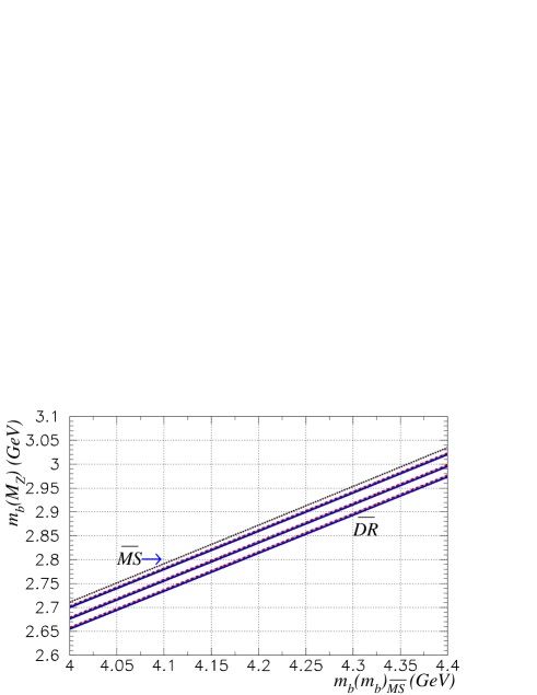
Figure 1: $m_{b}(M_{Z})$ as a function of $m_{b}^{\overline{\rm MS}}(m_{b})$. The solid lines show the results for $m_{b}^{\overline{\rm DR}}(M_{Z})$ using the first procedure described in the text, where we first run $m_{b}^{\overline{\rm MS}}$ to $M_{Z}$, and then convert to the $\overline{\rm DR}$ mass at the same scale. The lines correspond from top to bottom to values of $\alpha_{s}(M_{Z})_{\overline{\rm MS}}=0.1152,0.1172,0.1192$. The dashed lines show the corresponding results when we first convert to the $\overline{DR}$ scheme, and then evolve to $Q=M_{Z}$. Finally, the dotted line shows the value of $m_{b}^{\overline{\rm MS}}(M_{Z})$ for $\alpha_{s}(M_{Z})_{\overline{\rm MS}}=0.1172$.

An alternative approach would be to derive $m_{b}^{\overline{\rm DR}}(m_{b})$ using Eq. (11) and then evolve it to $Q=M_{Z}$ using Eq. (8). If we do so, we obtain the dashed lines in the figure. The relative difference between these and the solid lines is similar to the size of the three loop term in Eq. (5). The agreement between the dashed and solid lines provides additional evidence for the reliability of our procedure.

IV Summary

In summary, we have suggested a procedure to convert the value of $m_{b}^{\overline{\rm MS}}(m_{b})$ that is extracted from experimental data to $m_{b}^{\overline{\rm DR}}(M_{Z})$. This value serves as an important input for SUSY analyses with large $\tan\beta$.

Our main results are summarized in Fig. 1. Most of the recent analyses indicate mass that $m_{b}^{\overline{\rm MS}}(m_{b})=4.2\pm 0.1~{}{\rm GeV}$. This translates to $m_{b}^{\overline{\rm DR}}(M_{Z})=2.83\pm 0.11$ GeV. If instead we take the Particle Data Group range  Groom:in $4.0-4.4$ GeV for $m_{b}^{\overline{\rm MS}}(m_{b})$, the range of $m_{b}^{\overline{\rm DR}}(M_{Z})$ extends from $2.65-3.03$ GeV.

Acknowledgments

We thank M. Kalmykov for instructive correspondence, and C. Balázs, A. Belyaev and T. Blazek for helpful discussion. This research was supported in part by the U.S. Department of Energy under grants DE-FG03-94ER40833, DE-FG02-97ER41022 and DE-AC03-76-SF00515.

References

- (1) For recent reviews, see e.g. S. Martin, in Perspectives on Supersymmetry, edited by G. Kane (World Scientific), [hep-ph/9709356]; M. Drees, [hep-ph/9611409]; J. Bagger, [hep-ph/9604232]; X. Tata, Proc. IX J. Swieca Summer School, J. Barata, A. Malbousson and S. Novaes, Eds., [hep-ph/9706307]; S. Dawson, Proc. TASI 97, J. Bagger, Ed., [hep-ph/9712464].
- (2) Some examples include, D. Pierce et al. Nucl. Phys. B491, 3 (1997); E-Proc. RADCOR 2000, H. Haber, Editor, http://www.slac.stanford.edu/econf/C000911/; Radiative Corrections: Application of Quantum Field Theory to Phenomenology, Proc. RADCOR 98, J. Sola, Editor (World Scientific, 1999); Quantum Effects in the Minimal Supersymmetric Standard Model, Proc. Int. Workshop on the MSSM, Barcelona, Spain, 1997, J.Sola, Editor (World Scientific, 1997); J. Sola, Pramana 51, 239 (1998); W. Hollik and C. Schappacher, Nucl. Phys. B545, 98 (1999); D. Garcia and J. Sola, Phys. Lett. B357, 349 (1995); D. Garcia, J. Jiminez and J. Sola, Phys. Lett. B347, 309 (1995) and 347, 321 (1995).
- (3) Some representative examples include, M. Díaz and D. Ross, hep-ph/0205257 (2002); J. Gausch, W. Hollik and J. Sola, Phys. Lett. B510, 211 (2001); W. Beenakker, T. Blank and W. Hollik, hep-ph/0011092 (2000); R. Hopker, M. Spira and P.M. Zerwas, Nucl. Phys. B492, 51 (1997); W. Beenakker, R. Hopker, and P.M. Zerwas, Phys. Lett. B378, 159 (1996); E. Berger, M. Klasen and T. Tait, Phys. Rev. D62, 095014 (2000); M. Berger, B. Harris, M. Klasen and T. Tait, hep-ph/9903237 (1999); W. Beenakker et al. Phys. Rev. Lett. 83, 3780 (1999); M. A. Diaz, S. F. King and D. A. Ross, Nucl. Phys. B 529, 23 (1998); H. Eberl, A. Bartl and W. Majerotto, Nucl. Phys. B 472, 481 (1996).
- (4) R. Hempfling, Phys. Rev. D49, 6168 (1994); L. Hall, R. Rattazzi and U. Sarid, Phys. Rev. D50, 7048 (1994); M. Carena et al. Nucl. Phys. B426, 269 (1994);. Rattazzi and U. Sarid, Phys. Rev. D53, 1553 (1996).
- (5) H. Baer et al. Phys. Rev. Lett. 79, 986 (1997); ibid 80, 642 (1998) (E) (1997); H. Baer et al. Phys. Rev. D58, 075008 (1998); H. Baer et al. Phys. Rev. D59, 055014 (1999).
- (6) V. Barger, M. Berger and P. Ohmann, Phys. Rev. D49, 4908 (1994); M. Carena and C. Wagner, CERN-TH-7321 (1994); H. Murayama, M. Olechowski and S. Pokorski, Phys. Lett. B371, 57 (1996).
- (7) Y. Fukuda et al. Phys. Rev. Lett. 82, 2644 (1999) and 85, 3999 (2000).
- (8) H. Baer et al., Phys. Rev. D61, 111701 (2000); and D63, 015007 (2000); H. Baer and J. Ferrandis, Phys. Rev. Lett. 87, 211803 (2001).
- (9) T. Blazek, R. Dermisek and S. Raby, Phys. Rev. Lett. 88, 111804 (2002) and hep-ph/0201081 (2002), and references therein.
- (10) W. Siegel, Phys. Lett. B 84, 193 (1979).
- (11) K. Melnikov and A. Yelkhovsky, Phys. Rev. D59, 114009 (1999); A.H. Hoang, Phys. Rev. D61, 034005 (2000); M. Beneke and A. Signer, Phys. Lett. B471, 233 (1999); A. A. Penin and A. A. Pivovarov, Nucl. Phys. B549, 217 (1999).
- (12) D. E. Groom et al. [Particle Data Group Collaboration], Eur. Phys. J. C15 (2000) 1.
- (13) Here, and in the remainder of the text, the function is evaluated at the scale equal to the running mass; i.e. we drop the superscript on the argument of the function.
- (14) See, for instance, H. Arason et al. Phys. Rev. D46, 3945 (1992); D. Pierce et al., Ref. pierce ; L. Hall et al., Ref. carena .
- (15) At the Frontier of Particle Physics: Handbook of QCD, M. Shifman, Editor (World Scientific, 2001).
- (16) R. Tarrach, Nucl. Phys. B183, 384 (1981).
- (17) N. Gray, D. J. Broadhurst, W. Grafe and K. Schilcher, Z. Phys. C48, 673 (1990).
- (18) J. Fleischer, F. Jegerlehner, O. V. Tarasov and O. L. Veretin, Nucl. Phys. b539, 671 (1999) [Erratum-ibid. B571, 511]
- (19) K. G. Chetyrkin and M. Steinhauser, Nucl. Phys. B573, 617 (2000)
- (20) K. G. Chetyrkin, J. H. Kuhn and M. Steinhauser, Comp. Phys. Comm. 133, 43 (2000)
- (21) K. Melnikov and T. v. Ritbergen, Phys. Lett. B482, 99 (2000)
- (22) L. V. Avdeev and M. Y. Kalmykov, Nucl. Phys. B502, 419 (1997)
- (23) O. V. Tarasov, A. A. Vladimirov and A. Y. Zharkov, Phys. Lett. B 93 (1980) 429
- (24) K. G. Chetyrkin, Phys. Lett. B 404, 161 (1997)
- (25) J. A. Vermaseren, S. A. Larin and T. van Ritbergen, Phys. Lett. B405, 327 (1997)
- (26) K. G. Chetyrkin, B. A. Kniehl and M. Steinhauser, Phys. Rev. Lett. 79, 2184 (1997)
- (27) I. Antoniadis, C. Kounnas and K. Tamvakis, Phys. Lett. B 119, 377 (1982).
- (28) Analogous reasoning also provides an understanding why terms appear in the relations between the pole mass and short distance masses.
- (29) P. Abreu et al., Phys. Lett. B418, 430 (1998).