June 24, 2002 LBNL-50718

Electroweak Data and the Higgs Boson Mass:
A Case for New Physics

Michael S. Chanowitz

Theoretical Physics Group
Ernest Orlando Lawrence Berkeley National Laboratory
University of California
Berkeley, California 94720

Because of two $3\sigma$ anomalies, the Standard Model (SM) fit of the precision electroweak data has a poor confidence level, $CL=0.010$. Since both anomalies involve challenging systematic issues, it might appear that the SM could still be valid if the anomalies resulted from underestimated systematic error. Indeed the $CL$ of the global fit could then increase to 0.65, but that fit predicts a small Higgs boson mass, $m_{H}=43$ GeV, that is only consistent at $CL=0.035$ with the lower limit, $m_{H}>114$ GeV, established by direct searches. The data then favor new physics whether the anomalous measurements are excluded from the fit or not, and the Higgs boson mass cannot be predicted until the new physics is understood. Some measure of statistical fluctuation would be needed to maintain the validity of the SM, which is unlikely by broad statistical measures. New physics is favored, but the SM is not definitively excluded.

Disclaimer

This document was prepared as an account of work sponsored by the United States Government. While this document is believed to contain correct information, neither the United States Government nor any agency thereof, nor The Regents of the University of California, nor any of their employees, makes any warranty, express or implied, or assumes any legal liability or responsibility for the accuracy, completeness, or usefulness of any information, apparatus, product, or process disclosed, or represents that its use would not infringe privately owned rights. Reference herein to any specific commercial products process, or service by its trade name, trademark, manufacturer, or otherwise, does not necessarily constitute or imply its endorsement, recommendation, or favoring by the United States Government or any agency thereof, or The Regents of the University of California. The views and opinions of authors expressed herein do not necessarily state or reflect those of the United States Government or any agency thereof, or The Regents of the University of California.

Lawrence Berkeley National Laboratory is an equal opportunity employer.

1. Introduction

A decade of beautiful experiments at CERN, Fermilab, and SLAC have provided increasingly precise tests of the Standard Model (SM) of elementary particle physics. The data is important for two reasons: it confirms the SM at the level of virtual quantum effects and it probes the mass scale of the Higgs boson, needed to complete the model and provide the mechanism of mass generation. In the usual interpretation the data is thought to constrain the Higgs boson mass, $m_{H}$, most recently with $m_{H}<195$ GeV[1] at confidence level $CL=95\%$. At the same time direct searches for the Higgs boson at LEP II have established a 95% $CL$ lower limit, $m_{H}>114$ GeV.[2]

Recently the agreement of the precision data with the SM has moved from excellent to poor. For the global fits enumerated below, the confidence level has evolved from 0.45 in the Summer of 1998,[4] to 0.04 in the Spring of 2001,[5] and then to 0.010 in the current Spring 2002 data.[1] The current low $CL$ is a consequence of two $3\sigma$ anomalies, together with the evolution of the $W$ boson mass measurement, as shown below. The $3\sigma$ anomalies are (1) the discrepancy between the SM determination of $x_{W}^{l}={\rm sin}^{2}\theta^{l}_{W}$, the effective leptonic weak interaction mixing angle, from three hadronic asymmetry measurements, $x_{W}^{l}[A_{H}]$, versus its determination from three leptonic measurements, $x_{W}^{l}[A_{L}]$, and (2) the NuTeV measurement of charged and neutral current (anti)neutrino-nucleon scattering,[6] quoted as an effective on-shell weak interaction mixing angle, $x_{W}^{\rm OS}[\stackrel{{\scriptstyle(-)}}{{\nu}}N]$.

If either anomaly is genuine, it indicates new physics, the SM fit is invalidated, and we cannot use the precision data to constrain the Higgs boson mass until the new physics is understood. However both anomalous measurements involve subtle systematic issues, concerning experimental technique and, especially, nontrivial QCD-based models. If the systematic uncertainties were much larger than current estimates, the $CL$ of the global fit could increase to as much as 0.65, as shown below. It is then possible to imagine that the SM might still provide a valid description of the data and a useful constraint on the Higgs boson mass.

We will see however that this possibility is unlikely, because of a contradiction that emerges between the resulting global fit and the 95% $CL$ lower limit, $m_{H}>114$ GeV. The central point is that the anomalous measurements are the only $m_{H}$-sensitive observables that place the Higgs boson mass in the region allowed by the searches. All other $m_{H}$-sensitive observables predict $m_{H}$ far below 114 GeV. We find that if the anomalous measurements are excluded, the confidence level for $m_{H}>114$ GeV from the global fit is between 0.030 and 0.035, depending on the method of estimation.

The hypothesis that the anomalies result from systematic error then also favors new physics, in particular, new physics that would raise the prediction for $m_{H}$ into the experimentally allowed region. This can be accomplished, for example, by new physics whose dominant effect on the low energy data is on the $W$ and $Z$ vacuum polarizations (i.e., “oblique”[7]), as shown explicitly below. Essentially any value of $m_{H}$ is allowed in these fits.

It should be clear that our focus on the possibility of underestimated systematic error is not based on the belief that it is the most likely explanation of the data. In fact, the situation is truly puzzling, and there is no decisive reason to prefer systematic error over new physics as the explanation of either anomaly. Rather we have considered the systematic error hypothesis in order to understand its implications, finding that it also points to new physics.

The SM is then disfavored whether the experimental anomalies are genuine or not. The viability of the SM fit and the associated constraint on $m_{H}$ can only be maintained by invoking some measure of statistical fluctuation, perhaps in combination with a measure of increased systematic uncertainty. This is a priori unlikely by broad statistical measures discussed below, but it is not impossible. The conclusion is that the SM is disfavored but not definitively excluded. A major consequence is that it is important to search for the Higgs sector over the full range allowed by unitarity,[8] as, fortunately, we will be able to do at the LHC operating at its design luminosity.[9]

This paper extends and updates a previously published report,[10] based on the Spring 2001 data set, which focused exclusively on the $m_{H}$-sensitive observables. The present analysis is based on the Spring 2002 data, and considers $m_{H}$-sensitive observables as well as global fits of all $Z$-pole observables. The data has also changed in some respects: the $3\sigma$ NuTeV anomaly is a new development and the discrepancy between the hadronic and leptonic determinations of $x_{W}^{l}$ has diminished from 3.6 to 3.0$\sigma$. However the other $m_{H}$-sensitive observables are unchanged, and the present conclusions are consistent with the previous report.

Since in this work we also consider global fits, we can summarize the conclusion quantitatively by introducing the combined probability

$$P_{C}=CL({\rm Global\ Fit})\times CL(m_{H}>114).$$

The internal consistency of the global fit and its consistency with the search limit are independent constraints, so the combined likelihood to satisfy both is given by $P_{C}$. We find that $P_{C}$ is roughly independent of whether the three hadronic front-back asymmetry measurements are included in the fit, although the two factors on the right hand side of eq. (1.1) vary considerably in the two cases. For instance, for the global fit to ‘all’ data, we have $CL({\rm Global\ Fit})=0.010$ and $CL(m_{H}>114)=0.30$ so that $P_{C}=0.010\times 0.30=0.0030$. If the three hadronic asymmetry measurements are omitted we have instead $CL({\rm Global\ Fit})=0.066$, $CL(m_{H}>114)=0.047$, and $P_{C}=0.066\times 0.047=0.0031$. The extent of the agreement in this example is accidental, but the point remains approximately valid: if the three hadronic asymmetry measurements are omitted, the increase in the global fit confidence level is approximately compensated by a corresponding decrease in the confidence level that the fit is consistent with the direct search limit.

In section 2 we review the data used in the fits, with a discussion of how it has evolved during the past few years which emphasizes the importance of the $W$ mass measurement. In section 3 we briefly discuss the three generic explanations — statistics/systematics/new physics — of the discrepancies in the global SM fit. In section 4 we review the methodology of the SM fits and the choice of observables. In section 5 we present fits of the data which exhibit the range in $m_{H}$ preferred by the $m_{H}$-sensitive observables, as well as global fits with and without the anomalous measurements. In these fits we use the $\chi^{2}$ distribution for the global fits and the $\Delta\chi^{2}$ method to assess the consistency of the fits with the direct search lower limit on $m_{H}$. In section 6 we use a “Bayesian” maximimum likelihood method instead of $\Delta\chi^{2}$ to estimate the $CL$ for consistency with the direct searches. Section 7 illustrates the possible effect of new physics in the oblique approximation. The results are discussed in section 8.

2. The Data

We consider 13 $Z$-pole observables and in addition the directly measured values of $m_{W}$, the $W$ boson mass, $m_{t}$, the top quark mass, $\Delta\alpha_{5}$, the hadronic contribution to the renormalization of the electromagnetic coupling at the $Z$ pole, and the NuTeV result. As discussed in section 4, we do not include the $W$ boson width or the Cesium atomic parity violation measurement, which is the principal reason for the small differences between the global fits presented here and in [1]. These measurements have only recently been added to the global fits; they were not included in the 1998 and 2001 fits[4, 5] which we also consider below. Our all-data fit is tabulated in table 2.1, with the current preliminary experimental values from [1]. Details of the fitting procedure are given in section 4.

The central value for $x_{W}^{\rm OS}[\stackrel{{\scriptstyle(-)}}{{\nu}}N]$ from the NuTeV experiment is shown in table 2.1. In our SM fits we include the small dependence of $x_{W}^{\rm OS}[\stackrel{{\scriptstyle(-)}}{{\nu}}N]$ on $m_{t}$ and $m_{H}$ given in [6]. Table 2.1 also contains the model independent NuTeV result[6], given in terms of effective $Zqq$ couplings, $g_{L}^{2}=g_{uL}^{2}+g_{dL}^{2}$ and $g_{R}^{2}=g_{uR}^{2}+g_{dR}^{2}$. They are not included in the SM fits but are used instead of $x_{W}^{\rm OS}[\stackrel{{\scriptstyle(-)}}{{\nu}}N]$ in the new physics fits of section 7.

The confidence level of the SM fit in table 2.1 is poor, $CL=0.010$, with $\chi^{2}/N=27.7/13$. The central value of the Higgs boson mass is $m_{H}=94$ GeV. As shown in section 4, our results agree very well with those of [1] when we fit the same set of observables.

The SM fit was excellent in 1998 and has now become poor. Large discrepancies occur among the six SM determinations of the effective leptonic weak interaction mixing angle, $x_{W}^{l}$. The three leptonic measurements, $A_{LR}$, $A_{FB}^{l}$, and $A_{e,\tau}$ are quite consistent with one another. They combine with $\chi^{2}/N=1.6/2$, $CL=0.45$, to yield

$$x_{W}^{l}[A_{L}]=0.23113(21).$$

The three hadronic measurements are also mutually consistent and combine, with $\chi^{2}/N=0.03/2$ and $CL=0.985$, to yield

$$x_{W}^{l}[A_{H}]=0.23220(29).$$

But $x_{W}^{l}[A_{L}]$ and $x_{W}^{l}[A_{H}]$ differ by 2.99$\sigma$ corresponding to $CL=0.0028$. Combining (2.1) and (2.2), the result for all six measurements is $x_{W}^{l}=0.23149(17)$. The very small $\chi^{2}$ associated with the three hadronic measurements is either a fluctuation or it suggests that the errors are overestimated, in which case the discrepancy between $x_{W}^{l}[A_{L}]$ and $x_{W}^{l}[A_{H}]$ would be even greater.

The discrepancy between $x_{W}^{l}[A_{L}]$ and $x_{W}^{l}[A_{H}]$ is driven by the difference of the two most precise measurements, $A_{LR}$ and $A_{FB}^{b}$, which has been a feature of the data since the earliest days of LEP and SLC. At present, $x_{W}^{l}$ from $A_{LR}$ and $A_{FB}^{b}$ are respectively 0.23098(26) and 0.23218(31). They differ by 2.97$\sigma$, $CL=0.0030$, and combine to yield $x_{W}^{l}=0.23151(20)$.

Combining all 6 measurements directly we find $x_{W}^{l}=0.23149(17)$ as above, with $\chi^{2}/N=10.6/5$ and $CL=0.06$. Notice that the ratio of this confidence level to the confidence level, $CL=0.003$, for $x_{W}^{l}[A_{L}]$ versus $x_{W}^{l}[A_{H}]$, 0.06/0.003 = 20, is just the number of ways that two sets of three can be formed from a collection of 6 objects. If one attaches an a priori significance to the leptonic and hadronic subsets, then the appropriate confidence level is 0.003, from the combination of $x_{W}^{l}[A_{L}]$ and $x_{W}^{l}[A_{H}]$. If instead one regards the grouping into $x_{W}^{l}[A_{L}]$ and $x_{W}^{l}[A_{H}]$ as one of 20 random choices, then 0.06 is the appropriate characterization of the consistency of the data. In either case the consistency is problematic.

The determination of $x_{W}^{l}$ from the hadronic asymmetries assumes that the hadronic $Zq\overline{q}$ interaction vertices are given by the SM. For instance, to obtain $x_{W}^{l}$ from

$$A_{FB}^{b}={3\over 4}A_{b}A_{e}$$

we assume that $A_{b}$ is at its SM value, $A_{b}=A_{b}[{\rm SM}]$. $A_{b}[{\rm SM}]$ has very little sensitivity to the unknown value of $m_{H}$, and not much sensitivity to the other SM parameters either. $x_{W}^{l}$ is then obtained from $A_{e}=(g_{eL}^{2}-g_{eR}^{2})/(g_{eL}^{2}+g_{eR}^{2})$, using $g_{eL}={-1\over 2}+x_{W}^{l}$ and $g_{eR}=x_{W}^{l}$. The only assumption in obtaining $x_{W}^{l}$ from the leptonic asymmetries is lepton flavor universality.

The $3\sigma$ discrepancy between $x_{W}^{l}[A_{L}]$ and $x_{W}^{l}[A_{H}]$ is significant for three reasons. First, it is a failed test for the SM, since it implies $A_{q}\neq A_{q}[{\rm SM}]$. For instance, $A_{b}$ extracted from $A_{FB}^{b}$ (taking $A_{l}$ from the three leptonic asymmetry measurements) disagrees with $A_{b}[{\rm SM}]$ by 2.9$\sigma$, $CL=0.004$. Second, together with the $m_{W}$ measurement, the $x_{W}^{l}[A_{L}]$ – $x_{W}^{l}[A_{H}]$ discrepancy marginalizes the global SM fit, even without the NuTeV result. Finally, in addition to the effect on the global fit, it is problematic that the determination of the Higgs boson mass is dominated by the low probability combination of $x_{W}^{l}[A_{L}]$ and $x_{W}^{l}[A_{H}]$, or by the low probablility combination of the six asymmetry measurements. In judging the reliability of the prediction for $m_{H}$ we are concerned not only with the quality of the global fit but also with the consistency of the smaller set of measurements that dominate the $m_{H}$ prediction.

To understand the effect on the global fit it is useful to consider the evolution of the data from 1998[4] to the present[1], shown in table 2.2, together with the intervening Spring ’01 data set[5], on which [10] was based. The $x_{W}^{l}[A_{L}]$ – $x_{W}^{l}[A_{H}]$ discrepancy evolved from 2.4$\sigma$ in ’98 to 3.6$\sigma$ in Spring ’01 to 3.0$\sigma$ in Spring ’02. Excluding NuTeV, the $CL$ of the set of measurements listed in table 2.1 evolved during that time from a robust 0.46 to 0.04 to 0.10.

The decrease in the global $CL$ is only partially due to the changes in the asymmetry measurements. An equally important factor is the evolution of $m_{W}$, for which the precision improved dramatically, by a factor of 3, while the central value increased by ${1\over 2}\sigma$ with respect to the ’98 measurement. To understand the role of $m_{W}$, table 2.3 shows fits based on the current data plus two hypothetical scenarios in which all measurements are kept at their Spring ’02 values except $m_{W}$. In the first of these, $m_{W}$ is held at its ’98 central value and precision. In the second the current precision is assumed but with a smaller central value, corresponding to a ${1\over 2}\sigma$ downward fluctuation of the ’98 measurement. For both hypothetical data sets, the global $CL$ is greater by a factor two than the $CL$ of the current data.

To understand how $m_{W}$ correlates with the asymmetry measurements we also exhibit the corresponding fits in which either $A_{FB}^{b}$ or $A_{LR}$ are excluded. In the current data, the $CL$ increases appreciably, to 0.51, if $A_{FB}^{b}$ is excluded but much less if $A_{LR}$ is excluded, reflecting the larger pull of $A_{FB}^{b}$ in the SM fit. In the two hypothetical scenarios the $CL$ increases comparably whether $A_{LR}$ or $A_{FB}^{b}$ is excluded.

There are two conclusions from this exercise. First, the evolution of the $m_{W}$ measurement contributes as much to the marginalization of the global fit as does the evolution of the asymmetry measurements. Second, at its current value and precision $m_{W}$ tilts the SM fit toward $A_{LR}$ and $x_{W}^{l}[A_{L}]$, while tagging $A_{FB}^{b}$ and $x_{W}^{l}[A_{H}]$ as ‘anomalous’. The reason for this “alliance” of $m_{W}$ and $x_{W}^{l}[A_{L}]$ will become clear in section 5, where we will see that $m_{W}$ and $x_{W}^{l}[A_{L}]$ favor very light values of the Higgs boson mass, far below the 114 GeV lower limit, while $x_{W}^{l}[A_{H}]$ favors much heavier values, far above 114 GeV.

Returning to table 2.2, we also see the effect on the global fit of the new result from NuTeV. In the ’98 and ’01 data sets, NuTeV had little effect on the global $CL$. In the current data set, because of its increased precision and central value, it causes the $CL$ to decrease from an already marginal 0.10 to a poor 0.010. The low confidence level of the global SM fit is then due in roughly equal parts to 1) the discrepancy between the $x_{W}^{l}[A_{L}]$–$m_{W}$ alliance versus $x_{W}^{l}[A_{H}]$, and 2) the NuTeV result. We will refer to $x_{W}^{l}[A_{H}]$ and $x_{W}^{\rm OS}[\stackrel{{\scriptstyle(-)}}{{\nu}}N]$ as “anomalous” simply as a shorthand indication of their deviation from the SM fit, with no judgement intended as to their bona fides.

3. Interpreting the Discrepancies

In this section we wish to set the context for the fits to follow by briefly discussing the three generic explanations of the discrepancies in the SM fit reviewed in the previous section. They are statistical fluctuation, new physics, and underestimated systematic error. Combinations of the three generic options are also possible.

3.1 Statistical Fluctuations

One or both anomalies could be the result of statistical fluctuations. However, if the data is to be consistent not only with the global fit but also with the lower limit on $m_{H}$ from the Higgs boson searches as discussed in sections 5 and 6, it is necessary that both anomalous and non-anomalous measurements have fluctuated. If only the anomalous measurements were to have fluctuated, the global fit would improve but the conflict with the lower limit on $m_{H}$ would be exacerbated.

A high energy physics sage is reputed to have said, only partly in jest, that “The confidence level for $3\sigma$ is fifty-fifty.” The wisdom of the remark has its basis in two different phenomena. First, at a rate above chance expectation, many unusual results are ultimately understood to result from systematic error — this possibility is discussed below and its implications are explored in sections 5 and 6. Second, estimates of statistical significance are sometimes not appropriately defined. For instance, when a $3\sigma$ “glueball” signal is discovered over an appreciable background in a mass histogram with 100 bins, the chance likelihood is not the nominal 0.0027 associated with a $3\sigma$ fluctuation but rather the complement of the probability that none of the 100 bins contain such a signal, which is $1-0.9973^{100}=0.24$. The smaller likelihood is relevant only if we have an a priori reason to expect that the signal would appear in the very bin in which it was discovered.

In assessing the possibility of statistical fluctuations as the explanation of the poor SM fit, it should be clear that the global fit $CL$’s are appropriately defined, reflecting statistical ensembles that correspond to replaying the previous decade of experiments many times over. In particular, the $\chi^{2}$ $CL$’s of the global fits are like the glueball example with the significance normalized to the probability that the signal might emerge in any of the 100 bins, as shown explicitly below.

Table 3.1 summarizes $\chi^{2}$ fits of four different data sets, in which none, one, or both sets of anomalous measurements are excluded. Consider for instance fit B in which only $x_{W}^{\rm OS}[\stackrel{{\scriptstyle(-)}}{{\nu}}N]$ is excluded, with $CL=0.10$. In that fit, consisting of 16 measurements, the only significantly anomalous measurement is $A_{FB}^{b}$, with a pull of 2.77, for which the nominal $CL$ is 0.0056. The likelihood that at least one of 16 measurements will differ from the fit by $\geq 2.77\sigma$ is then $1-0.9944^{16}=0.09$, which matches nicely with the $\chi^{2}$ $CL$ of 0.10. Similarly, in fit C which retains NuTeV while excluding the hadronic asymmetry measurements, the outstanding anomaly is $x_{W}^{\rm OS}[\stackrel{{\scriptstyle(-)}}{{\nu}}N]$ with a pull of 3.0, and the probability for at least one such deviant is $1-0.9973^{14}=0.04$, compared to the $\chi^{2}$ $CL=0.05$. Finally, for the full data set, fit A, the outstanding anomalies are $x_{W}^{\rm OS}[\stackrel{{\scriptstyle(-)}}{{\nu}}N]$ with a pull of 3.0 and $A_{FB}^{b}$ with a pull of 2.55. In that case we ask for the probability of at least one measurement diverging by $\geq 3.0\sigma$ and a second by $\geq 2.55\sigma$, which is given by $1-0.9973^{17}-17(1-0.9973)(0.9892)^{16}=0.006$, compared to the $\chi^{2}$ $CL$ of 0.010.

We see then that the $\chi^{2}$ $CL$’s appropriately reflect “the number of bins in the histogram,” and that the poor $CL$’s of these SM fits are well accounted for by the appropriately defined probabilities that the outlying anomalous measurements could have occurred by chance. The nominal $\chi^{2}$ confidence levels of the global fits are then reasonable estimates of the probability that statistical fluctuations can explain the anomalies, which we may characterize as unlikely but not impossible. Only fit D, with both anomalies removed, has a robust confidence level, $CL=0.65$. We refer to fit D as the “Minimal Data Set.” The results and pulls for this fit are shown in table 3.2.

This discussion does not reflect the fact that the anomalous measurements are all within the subset of measurements that dominate the determination of $m_{H}$. In that smaller subset of measurements, the significance of the anomalies is not fully reflected by the global $CL$’s. As concerns the reliability of the fits of $m_{H}$, there is a clear a priori reason to focus on the $m_{H}$-sensitive measurements. We therefore also consider fits in which the observables $O_{i}$ in equation (4.1) below are restricted to the measurements which dominate the determination of $m_{H}$. These are the six asymmetries, $m_{W}$, $\Gamma_{Z}$, $R_{l}$, and $x_{W}^{\rm OS}[\stackrel{{\scriptstyle(-)}}{{\nu}}N]$. (The $m_{H}$-insensitive measurements which are omitted from these fits are $\sigma_{h}$, $R_{b}$, $R_{c}$, $A_{b}$, and $A_{c}$.) The results of the corresponding fits, A^′ - D^′, are tabulated at the bottom of table 3.1. Except for the minimal data sets, D and D^′, in every other case the fit restricted to $m_{H}$-sensitive measurements has an appreciably smaller confidence level than the corresponding global fit. In addition to the problems of the global fits, the poorer consistency of this sector of measurements provides another cause for concern in assessing the reliability of the SM prediction of $m_{H}$.

3.2 New Physics

Each anomaly could certainly be the result of new physics. The NuTeV experiment opens a very different window on new physics than the study of on-shell $Z$ boson decays at LEP I and SLC.[11] For example, a $Z^{\prime}$ boson mixed very little or not at all with the $Z$ boson, could have little effect on on-shell $Z$ decay but a big effect on the NuTeV measurement, which probes a space-like region of four-momenta centered around $Q^{2}\simeq-20$ GeV². The strongest bounds on this possibility would come from other off-shell probes, such as atomic parity violation, $e^{+}e^{-}$ annihilation above the $Z$ pole, and high energy $p\overline{p}$ collisions.

New physics could also affect the hadronic asymmetry measurements. Here we can imagine two scenarios, depending on how seriously we take the clustering of the three hadronic asymmetry measurements. Taking it seriously, we would be led to consider leptophobic $Z^{\prime}$ models[12], as were invoked to explain the $R_{b}$ anomaly, which was subsequently found to have a systematic, experimental explanation.

Or we might regard the clustering of the three hadronic measurements as accidental. Then we would be led to focus on $A_{FB}^{b}$, by far the most precise of the three hadronic asymmetry measurements, and we could arrive at acceptable global fits by assuming new physics coupled predominantly to the third generation quarks. New physics would then account for the $A_{FB}^{b}$ anomaly, with an additional effect on the less precisely measured jet charge asymmetry, $Q_{FB}$. The third generation is a plausible venue for new physics, since the large top quark mass suggests a special connection of the third generation to new physics associated with the symmetry breaking sector.

Since $R_{b}\propto g_{bL}^{2}+g_{bR}^{2}$ while $A_{FB}^{b}\propto g_{bL}^{2}-g_{bR}^{2}$, and because $R_{b}$, which is more precisely measured than $A_{FB}^{b}$, is only $\sim 1\sigma$ from its SM value, some tuning of the shifts $\delta g_{bL}$ and $\delta g_{bR}$ is required to fit both measurements. The right-handed coupling must shift by a very large amount, with $\delta g_{bR}\gg\delta g_{bL}$ and $\delta g_{bR}\raisebox{-1.72218pt}{\hbox to0.0pt{$\sim$\hss}}\raisebox{1.72218pt}{$>$}0.1g_{bR}$. An effect of this size suggests new tree-level physics or radiative corrections involving a strong interaction.

Examples of tree-level physics are $Z\ -\ Z^{\prime}$ mixing or $b\ -\ Q$ mixing. A recent proposal to explain the $A_{FB}^{b}$ anomaly embeds a $Z^{\prime}$ boson in a right-handed $SU(2)_{R}$ extension of the SM gauge group in which the third generation fermions carry different $SU(2)_{R}$ charges than the first and second generations.[13] $Z^{\prime}$ bosons coupled preferentially to the third generation are generic in the context of topcolor models.[14] An explanation by $b\ -\ Q$ mixing, requires $Q$ to be a charge $-1/3$ quark with non-SM weak quantum numbers; this possibility has been explored in the context of the latest data in reference [15] and previously in [16].

If new physics explains the $A_{FB}^{b}$ anomaly, it must also affect $A_{b}$. If we use eq. (2.3) with the factor $A_{e}=0.1501(17)$ taken from the three leptonic asymmetry measurements (assuming lepton universality), we find that the experimental value $A_{FB}^{b}=0.0994(17)$ implies $A_{b}[A_{FB}^{b}]=0.883(18)$, which is $2.89\sigma$ from $A_{b}[{\rm SM}]=0.935$, $CL=0.004$. However $A_{b}$ is measured more directly at SLC by means of $A_{FBLR}^{b}$, the front-back left-right asymmetry. In the Summer of 1998 that measurement yielded $A_{b}[A_{FBLR}^{b}]=0.867(35)$, lower by $1.9\sigma$ than $A_{b}[{\rm SM}]$, lending support to the new physics hypothesis. But the current measurement, $A_{b}[A_{FBLR}^{b}]=0.922(20)$, is only $0.6\sigma$ below $A_{b}[{\rm SM}]$. It no longer bolsters the new physics hypothesis but it is also not grossly inconsistent with $A_{b}[A_{FB}^{b}]$, from which it differs by $1.44\sigma$, $CL=0.15$. Combining $A_{b}[A_{FB}^{b}]$ and $A_{b}[A_{FBLR}^{b}]$ we find $A_{b}[A_{FBLR}^{b}\oplus A_{FBLR}^{b}]=0.900(13)$, which differs from the SM by $2.69\sigma$, $CL=0.007$. Thus while the $A_{FBLR}^{b}$ measurement no longer supports the new physics hypothesis, it also does not definitively exclude it.

If either anomaly is the result of new physics, the SM fails and we cannot predict the Higgs boson mass until the nature of the new physics is understood. New physics affecting the NuTeV measurement and/or the hadronic asymmetry measurements will certainly change the relationship between those observables and the value of $m_{H}$, and could affect other observables in ways that change their relationships with $m_{H}$.

3.3 Systematic Uncertainties

The two $3\sigma$ anomalies each involve subtle systematic issues, having to do both with performance of the measurements and the interpretation of the results. With respect to interpretation, both use nonperturbative QCD models with uncertainties that are difficult to quantify. In both cases the experimental groups have put great effort into understanding and estimating the systematic uncertainties. Here we only summarize the main points.

The central value for the NuTeV SM result is $x_{W}^{\rm OS}(\stackrel{{\scriptstyle(-)}}{{\nu}}N)=0.2277\pm 0.0013({\rm statistical})\pm 0.0009({\rm systematic})$. The estimated systematic error consists in equal parts of an experimental component, $\pm 0.00063$, and a modelling component, $\pm 0.00064$. Uncertainty from the $\nu_{e}$ and $\overline{\nu}_{e}$ fluxes makes the largest single contribution to the experimental component, $\pm 0.00039$, with the remainder comprised of various detector-related uncertainties. The modelling uncertainty is dominated by nonperturbative nucleon structure, with the biggest component, $\pm 0.00047$, due to the charm production cross section.

Two possible nonperturbative effects have been considered (see [17, 11, 18] and references therein). One is an asymmetry in the nucleon strange quark sea, $\int x(s(x)-\overline{s}(x))\>dx\neq 0$. Using dimuons from the separate $\nu$ and $\overline{\nu}$ beams, the NuTeV collaboration finds evidence for a $-10\%$ asymmetry within the NuTeV cross section model. If truly present, it would increase the discrepancy from 3.0 to 3.7$\sigma$.[17] For consistency with the SM, an asymmetry of $\simeq+30\%$ would be needed.

A second possible nonperturbative effect is isospin symmetry breaking in the nucleon wave function, $d^{p}(x)\neq u^{n}(x)$. Studies are needed to determine if structure functions can be constructed that explain the NuTeV anomaly in this way while maintaining consistency with all other constraints. A negative result could rule out this explanation, while a positive result would admit it as a possibility. Confirmation would then require additional evidence.

The $3\sigma$ discrepancy between $x_{W}^{l}[A_{L}]$ and $x_{W}^{l}[A_{H}]$ also raises the possibility of subtle systematic uncertainties. The determination of $x_{W}^{l}[A_{L}]$ from the three leptonic measurements, $A_{LR}$, $A_{FB}^{l}$, and $A_{e,\tau}$, involve three quite different techniques so that large, common systematic errors are very unlikely. The focus instead is on the hadronic measurements, $A_{FB}^{b}$, $A_{FB}^{c}$, and $Q_{FB}$. In these measurements, $b$ and $\overline{c}$ quarks are mutual backgrounds for one another. The signs of both the $A_{FB}^{b}$ and $A_{FB}^{c}$ anomalies are consistent with misidentifying $b\leftrightarrow\overline{c}$, although the estimated magnitude[19] of the effect is far smaller than what is needed. QCD models of charge flow and gluon radiation are a potential source of common systematic uncertainty for all three measurements. The two heavy flavor asymmetries, $A_{FB}^{b}$ and $A_{FB}^{c}$, have the largest error correlation of the heavy flavor $Z$-pole measurements, quoted as 16% in the most recent analysis.[1]

Since $x_{W}^{l}[A_{H}]$ is dominated by $x_{W}^{l}[A_{FB}^{b}]$, the greatest concern is the systematic uncertainties of $A_{FB}^{b}$. The combined result of the four LEP experiments is $A_{FB}^{b}=0.0994\pm 0.00157({\rm statistics})\pm 0.00071({\rm systematic})$. The systematic component arises from an “internal” (experimental) component of $\pm 0.00060$ and a “common” component of $\pm 0.00039$, where the latter is dominated by the $\pm 0.00030$ uncertainty ascribed to QCD corrections.[19]

3.4 Summary

It is not now possible to choose among the three generic explanations of the anomalies, except to say that statistical fluctuations are unlikely per the nominal $CL$ of the global fit. Bigger systematic errors could rescue the SM fit but would have to be much bigger than current estimates. Rather than further refinement of existing error budgets, this probably means discovering new, previously unconsidered sources of error. In this paper we focus on the systematic error hypothesis, not because we think it the most likely explanation — we do not — but, assuming it to be true, to see if it can really reconcile the SM with the data.

4. Methods

In this section we describe the methodology of the SM fits. We also discuss the choice of observables, which differs slightly from the choice made in [1].

We use ZFITTER v6.30[20] to compute the SM electroweak radiative corrections, with results that agree precisely (to 2 parts in $10^{5}$ or better) with those obtained in [1]. The input parameters are $m_{Z}$, $m_{t}$, the hadronic contribution to the renormalization of $\alpha$ at the $Z$-pole, $\Delta\alpha_{5}(m_{Z})$, the strong coupling constant at the $Z$-pole, $\alpha_{S}(m_{Z})$, and the Higgs boson mass, $m_{H}$. For any point in this five dimensional space ZFITTER provides the corresponding SM values of the other observables, $O_{i}$, listed in table 2.1.

To generate the $\chi^{2}$ distributions we scan over the four parameters, $m_{t}$, $\Delta\alpha_{5}(m_{Z})$, $\alpha_{S}(m_{Z})$, and $m_{H}$. For a specified collection of observables $O_{i}$, we then have

$$\chi^{2}=\left({m_{t}-m_{t}^{\rm EXPT}\over\Delta m_{t}^{\rm EXPT}}\right)^{2}+\left({\Delta\alpha_{5}-\Delta\alpha_{5}^{\rm EXPT}\over\Delta(\Delta\alpha_{5}^{\rm EXPT})}\right)^{2}+\sum_{i}\left({O_{i}-O_{i}^{\rm EXPT}\over\Delta O_{i}^{\rm EXPT}}\right)^{2}$$

The experimental values are given in table 2.1.

We do not scan over $m_{Z}$ but simply fix it at its central experimental value. Because $m_{Z}$ is so much more precise than the other observables, it would contribute negligibly to $\chi^{2}$ if we did scan on it. We have verified this directly by performing fits in which it was varied, with only negligible differences from the fits in which it is fixed at the central value. This can also be seen in the global fits reported by the EWWG, in which the pull from $m_{Z}$ is invariably much less than 1. In this case, inclusion of $m_{Z}$ has no effect on the $CL$ of the fit, because (1) the contribution to $\chi^{2}$ is negligible and (2) the scan on $m_{Z}$ has no effect on the number of degrees of freedom since it is both varied and constrained. Since it has little effect, we choose not to scan on $m_{Z}$ in order to facilitate the numerical calculations.

For $\Delta\alpha_{5}(m_{Z})$ we use the determination of [21], which incorporates the most recent $e^{+}e^{-}$ annihilation data and is also the default choice of [1]. In [10] we also presented results for four other determinations of $\Delta\alpha_{5}(m_{Z})$.

For the global fits $\alpha_{S}(m_{Z})$ is left unconstrained, as is also done in [1], because the $Z$-pole SM fit is itself the most precise determination of $\alpha_{S}(m_{Z})$. For the fits which consider more limited sets of observables, we use the following rule: if at least two of the three observables which dominate the the determination of $\alpha_{S}(m_{Z})$ (these are $\Gamma_{Z}$, $R_{l}$, and $\sigma_{h}$) are included in the fit, $\alpha_{S}$ is unconstrained as in the global fits. Otherwise we constrain it to 0.118(3). In any case, because the $m_{H}$-sensitive observables are predominantly $\alpha_{S}$-insensitive, the results we obtain for $m_{H}$ depend very little on the details of how $\alpha_{S}$ is specified.

The fits also include the important correlations from the error matrices presented in tables 2.3 and 5.3 of [1]. We retain the correlations that are $\geq 0.05$ in the $6\times 6$ heavy flavor error matrix, for $A_{FB}^{b}$, $A_{FB}^{c}$, $A_{b}$, $A_{c}$, $R_{b}$, and $R_{c}$. Similarly we retain correlations $\geq 0.05$ in the $4\times 4$ correlation matrix for $\Gamma_{Z}$, $\sigma_{h}$, $R_{l}$, and $A_{FB}^{l}$. These correlations shift the value of $\chi^{2}$ by as much as 2 units.

Our global fits differ slightly from the all-data fit of [1], principally because we use the set of measurements the Electroweak Working Group (EWWG) used through Spring 2001 but not two measurements that were subsequently added by the EWWG. From Summer 2001 the EWWG all-data fit included the Cesium atomic parity violation (APV) measurement, and in Spring 2002, the $W$ boson width, $\Gamma_{W}$, was included.

Reference [1] uses a 2001 determination of the Cesium APV measurement that has recently been superseded by newer results from the same authors[22]. With the average value from the more recent study, $Q_{W}=-72.18(46)$ (with experimental and theoretical errors combined in quadrature), and the SM value from [1], the pull is 1.6, rather than 0.6 as quoted in [1]. The effect on the all-data global fit in [1] is to change $\chi^{2}/N=28.8/15$, $CL=0.017$ to $\chi^{2}/N=30.8/15$, $CL=0.009$, decreasing the confidence level by a factor two. Rather than use the updated value, we choose not to include the Cs APV measurement since the theoretical systematic uncertainties are still in flux.

We choose not to include $\Gamma_{W}$ because it has not yet attained a level of precision precision approaching that of the other measurements in the fit. For instance, $\Gamma_{Z}$ is 30 times more precise than $\Gamma_{W}$, so that $\Gamma_{W}$ has 1/900’th the weight of $\Gamma_{Z}$ in the global fits. At the current precision it has no sensitivity to new physics signals of the order of magnitude probed by the other observables in the fit. Its effect on the fits of $m_{H}$, which are the principal concern of this work, is completely negligible.

In any case, the decision not to include the $\Gamma_{W}$ and APV measurements does not have a major effect on our results. In particular, the effect on the Higgs boson mass predictions is negligible. Furthermore, our all-data fit, with $CL=0.010$, has a very similar confidence level to that of the all-data fit of [1], $CL=0.009$, if the APV determination is updated to reflect [22].

We closely reproduce the results of [1] when we use the same set of observables. For instance, adding $\Gamma_{W}$ and $Q_{W}({\rm Cs})$ as specified in [1] to the observables in our global fit, table 2.1, we obtain $\chi^{2}/N=28.7/15$, $CL=0.018$, compared to $\chi^{2}/N=28.8/15$, $CL=0.017$ from the corresponding (all-data) fit of [1].

5. The $\chi^{2}$ Fits

In this section we present several SM fits of the data, using $\chi^{2}$ to estimate global $CL$’s and $\Delta\chi^{2}$ to obtain the constraints on the Higgs boson mass. The $\Delta\chi^{2}$ method, used also in [1], is defined as follows. Let $m_{\rm MIN}$ be the value of $m_{H}$ at the $\chi^{2}$ minimum, and let $m_{L}$ be an arbitrary mass such that $m_{L}>m_{\rm MIN}$. Then the confidence level $CL(m_{H}>m_{L})$ is one half of the confidence level corresponding to a $\chi^{2}$ distribution for one degree of freedom, with the value of the $\chi^{2}$ distribution given by $\Delta\chi^{2}=\chi^{2}(m_{L})-\chi^{2}(m_{\rm MIN})$. We consider both global fits and fits restricted to the $m_{H}$-sensitive observables.

In addition to $m_{t}$ and $\Delta\alpha_{5}$, which are input parameters to the ZFITTER calculations, the observables with the greatest sensitivity to $m_{H}$ are $x_{W}^{l}$ from the six asymmetry measurements, $m_{W}$, $\Gamma_{Z}$, $R_{l}$, and $x_{W}^{\rm OS}[\stackrel{{\scriptstyle(-)}}{{\nu}}N]$. It is useful to consider the domains in $m_{H}$ favored by these observables, in order to understand the “alliances” (see section 2) that shape the global fit, and to understand the consistency of the fits with the LEP II lower limit on $m_{H}$. In fits restricted to $m_{H}$-sensitive obervables, $\chi^{2}$ is given by eq. 4.1, where the $O_{i}$ are restricted to the $m_{H}$-sensitive observables under consideration. In addition, for fits containing fewer than two of the three $\alpha_{S}$-sensitive observables — $\Gamma_{Z}$, $R_{l}$, and $\sigma_{h}$ — we constrain $\alpha_{S}(m_{Z})$ by including it with the $O_{i}$ in equation (4.1) as discussed in section 4.

The experimental quantity that currently has the greatest sensitivity to $m_{H}$ is $x_{W}^{l}$, determined from the six asymmetry measurements. Figure 1 displays the distributions of the three individual leptonic measurements and the combined result from all three, $x_{W}^{l}[A_{L}]$; it shows that the upper limit is dominated by $A_{LR}$. The central value, $m_{H}=55$ GeV, symmetric 90% confidence interval, and likelihood $CL(m_{H}>114)$ are given in table 5.1. Note that the 95% upper limit is $m_{H}<143$ GeV.

Figure 2 shows that the $\chi^{2}$ distribution from $x_{W}^{l}[A_{H}]$ is completely dominated by the $b$ quark asymmetry, $A_{FB}^{b}$. The central value is $m_{H}=410$ GeV and the 95% lower limit is 145 GeV, just above the 95% upper limit from $x_{W}^{l}[A_{L}]$. The 95% upper limit extends above 1 TeV. Figure 3 shows the $\chi^{2}$ distributions of both $x_{W}^{l}[A_{L}]$ and $x_{W}^{l}[A_{H}]$, with the respective symmetric 90% confidence intervals indicated by the dot-dashed horizontal lines.

It is also interesting to isolate the effect of the $W$ boson mass measurement, because it is the second most important quantity for fixing $m_{H}$, and because it is a dramatically different measurement with a completely different set of systematic uncertainties. Figure 4 shows the $\chi^{2}$ distribution from $m_{W}$. The central value is $m_{H}=23$ GeV and the 95% upper limit is 121 GeV. Both $m_{W}$ and $x_{W}^{l}[A_{L}]$ then favor very light values of $m_{H}$. This is the basis of the “alliance” between $x_{W}^{l}[A_{L}]$ and $m_{W}$, discussed in section 2, that pushes $A_{FB}^{b}$ to outlyer status and contributes to the marginal confidence level of the SM fit.

The two other $Z$-pole observables with sensitivity to $m_{H}$ are $\Gamma_{Z}$ and $R_{l}$, which also involve different systematic uncertainties than the asymmetry measurements. The corresponding $\chi^{2}$ distributions are also plotted in figure 4, together with the combined distribution for $m_{W}$, $\Gamma_{Z}$ and $R_{l}$. $R_{l}$ also favors small $m_{H}$, with its $\chi^{2}$ minimum off the chart below 10 GeV. $\Gamma_{Z}$ is often represented as favoring $m_{H}\simeq{\rm O}(100)$ GeV, but we see in figure 4 and with the expanded scale in figure 5, that it actually has two nearly degenerate minima, at about 16 and 130 GeV. In table 5.1 we see that the combined distribution of the three non-asymmetry measurements has a central value at 13 GeV and a 95% upper limit at 73 GeV with $CL(m_{H})>114)=0.021$

Figure 6 shows the $\chi^{2}$ distribution from the NuTeV measurement, $x_{W}^{\rm OS}[\stackrel{{\scriptstyle(-)}}{{\nu}}N]$. The minimum lies above 3 TeV and the 95% lower limit is at $\simeq 660$ GeV. The SM fits the NuTeV anomaly by driving $m_{H}$ to very large values, but the new physics that actually explains the effect, if it is genuine, would not be so simply tied to the symmetry breaking sector but might for instance reflect an extension of the gauge sector, with implications for the symmetry breaking sector that cannot be foretold. In any case, as discussed in section 7, values of $m_{H}$ above $\sim 1$ TeV cannot be interpreted literally.

It is striking that the measurements favoring $m_{H}$ in the region allowed by the direct searches are precisely the ones responsible for the large $\chi^{2}$ of the global fit. They favor values far above 100 - 200 GeV while the measurements consistent with the fit favor values far below, as shown in the bottom two lines of table 5.1. The fit based on $x_{W}^{l}[A_{L}]\oplus m_{W}\oplus\Gamma_{Z}\oplus R_{l}$ (fit $D^{\prime}$ in table 3.1) has $m_{H}<106$ GeV at 95% $CL$, while the fit based on $x_{W}^{l}[A_{H}]\oplus x_{W}^{\rm OS}[\stackrel{{\scriptstyle(-)}}{{\nu}}N]$ has $m_{H}>220$ GeV at 95% $CL$. The corresponding $\chi^{2}$ distributions are shown in figure 7.

Next we consider the global fits that were discussed in section 3.1. The principal results are summarized in table 5.2. The “all-data” fit, fit A (shown in detail in table 2.1), closely resembles the all-data fit of [1], up to small differences arising from the slightly different choice of observables discussed in section 4. As summarized in table 5.2, the $\chi^{2}$ minimum is at $m_{H}=94$ GeV, with $CL(\chi^{2})=0.010$. The 95% upper limit is $m_{H}<193$ GeV and the consistency with the search limit is $CL(m_{H}>114\ {\rm GeV})=0.30$. The $\chi^{2}$ distribution is shown in figure 8, where the vertical dashed line denotes the direct search limit and the horizontal dot-dashed line indicates the symmetric 90% $CL$ interval. The combined likelihood for internal consistency of the fit and consistency between fit and search limit, defined in equation (1.1), is $P_{C}=0.0030$.

The “Minimal Data Set,” fit D, with $x_{W}^{\rm OS}[\stackrel{{\scriptstyle(-)}}{{\nu}}N]$ and $x_{W}^{l}[A_{H}]$ omitted, is shown in detail in table 3.2, and the $\chi^{2}$ distribution is shown in figure 8. The minimum is at $m_{H}=43$ GeV, with a robust confidence level $CL(\chi^{2})=0.65$. But the 95% upper limit is $m_{H}<105$ GeV and the consistency with the search limit is a poor $CL(m_{H}>114\ {\rm GeV})=0.035$. (The latter is nearly identical to the value 0.038 shown in table 5.1 for fit D^′, which is the corresponding fit restricted to $m_{H}$-sensitive observables, defined in section 3.1.) The combined likelihood for fit D is $P_{C}=0.023$.

In fit C with $x_{W}^{l}[A_{H}]$ omitted the $\chi^{2}$ minimum is at $m_{H}=45$ GeV with $CL(\chi^{2})=0.066$. The confidence level for consistency with the search limit is $CL(m_{H}>114\ {\rm GeV})=0.047$. The combined likelihood is $P_{C}=0.0031$.

Finally we consider fit B, with $x_{W}^{l}[A_{H}]$ retained and $x_{W}^{\rm OS}[\stackrel{{\scriptstyle(-)}}{{\nu}}N]$ omitted. Now the $m_{H}$ prediction is raised appreciably, with the $\chi^{2}$ minimum at $m_{H}=81$ GeV, but the quality of the fit is marginal, with $CL(\chi^{2})=0.10$. The confidence level for consistency with the search limit is more robust, $CL(m_{H}>114\ {\rm GeV})=0.26$, and the combined likelihood is $P_{C}=0.026$.

The effect of the hadronic asymmetries and the NuTeV measurement is apparent from table 5.2. The NuTeV measurement diminishes $CL(\chi^{2})$ by a factor 10, seen by comparing fit A with fit B and fit C with fit D, while its effect on $CL(m_{H}>114)$ is modest. Consequently the NuTeV measurement also diminishes the combined likelihood $P_{C}$ by an order of magnitude. Comparing fit A with fit C or fit B with fit D, we see that the hadronic asymmetries also diminish $CL(\chi^{2})$, by a factor $\sim 7$, but that they increase $CL(m_{H}>114)$ by a nearly identical factor, so that they have little effect on $P_{C}$.

6. “Bayesian” Maximum Likelihood Fits

The $\Delta\chi^{2}$ method for obtaining the confidence levels for different regions of $m_{H}$ is poweful and convenient but, at least to this author, not completely transparent. We have therefore also approached these estimates by constructing likelihood distributions as a function of $m_{H}$, varying the parameters to find the point of maximum likelihood for each value of $m_{H}$. Assuming Gaussian statistics, the log likelihood is

$$-{\rm log}({\cal L}(m_{H}))=C\chi^{2}(m_{H}),$$

so that the maximization of the likelihood is equivalent to the minimization of $\chi^{2}$. The proportionality constant $C$ is determined by the normalization condition for ${\cal L}$.

The method is “Bayesian” in the sense that the domain of normalization and the measure are specified by a priori choices that are guided by the physics. The likelihood distribution is normalized in the interval $10\>{\rm GeV}\>\leq\>m_{H}\>\leq\>3{\rm TeV}$,

$$\int^{m_{H}=3\>{\rm TeV}}_{m_{H}=10{\rm GeV}}d{\rm log}(m_{H}){\cal L}(m_{H})=1.$$

The choice of measure is motivated by the fact that ${\rm log}(m_{H})$ is approximately linearly proportional to the experimental parameters, which are assumed to be Gaussian distributed, such as $m_{t}$, $\Delta\alpha_{5}$ and the various $O_{i}$ — see for instance the interpolating formulae in [24]. The choice of interval is conservative in the sense that enlarging the domain above and below causes $CL(m_{H}>114{\rm GeV})$ to be even smaller than the results given below.

The normalized likelihood distributions for fits A and D, the all-data and Minimal Data Sets, are shown in figure 9, where we display both the differential and integrated distributions. The confidence level $CL(m_{H}>114)$ is the area under the differential distribution above 114 GeV. For the Minimal Data Set the result is $CL(m_{H}>114\ {\rm GeV})=0.030$, in good agreement with the result 0.035 obtained from $\Delta\chi^{2}$ in section 5. For the all-data set it is $CL(m_{H}>114\ {\rm GeV})=0.25$, compared with 0.30 from $\Delta\chi^{2}$.

It is clear from figure 9 that the likelihood distribution from the Minimal Data Set is vanishingly small at 3 TeV but has some support at 10 GeV. If we were to enlarge the domain in $m_{H}$ both above and below, the effect would be to further decrease the likelihood for $m_{H}>114$ GeV.

7. New Physics in the Oblique Approximation

If we assume the Minimal Data Set, the contradiction with the LEP II lower limit on $m_{H}$ is either a statistical fluctuation or a signal of new physics. Two recent papers provide examples of new physics that could do the job. Work by Altarelli et al.[25] in the framework of the MSSM finds that the prediction for $m_{H}$ can be raised into the region allowed by the Higgs boson searches if there are light sneutrinos, $\simeq 55$ – 80 GeV, light sleptons, $\simeq 100$ GeV, and moderately large tan$\>\beta\simeq 10$. This places the sleptons just beyond the present experimental lower limit, where they could be discovered in Run II at the TeVatron. A second proposal, by Novikov et al.,[26] finds that a fourth generation of quarks and leptons might also do the job, provided the neutrino has a mass just above $m_{Z}/2$. An illustrative set of parameters is $m_{N}\simeq 50$ GeV, $m_{E}\simeq 100$ GeV, $m_{U}+m_{D}\simeq 500$ GeV, $|m_{U}-m_{D}|\simeq 75$ GeV, and $m_{H}\simeq 300$ GeV.

In this section we do not focus on any specific model of new physics but consider the class of models that can be represented in the oblique approximation[27], parameterized by the quantities $S,T,U$.[7] The essential assumption is that the dominant effect of the new physics on the electroweak observables can be parameterized as effective contributions to the $W$ and $Z$ boson self energies. These contributions are not limited to loop corrections, since the oblique parameters can also represent tree level phenomena such as $Z-Z^{\prime}$ mixing.[28] We will restrict ourselves to the $S$ and $T$ parameters, since they suffice to make the point that oblique new physics can remove the contradiction between the Minimal Data Set and the search limit, leaving $m_{H}$ as an essentially free parameter. We also show that $S,T$ corrections do not improve the confidence levels of the global fits that include the anomalous measurements.

For the observables $O_{i}$ the oblique corrections are given by

$$dQ_{i}=\sum_{i}(A_{i}S+B_{i}T)$$

with $Q_{i}$ defined by $Q_{i}=O_{i}$ or $Q_{i}={\rm ln}(O_{i})$ as indicated in table 7.1 where $A_{i}$ and $B_{i}$ are tabulated. Since these are not SM fits, instead of $x_{W}^{\rm OS}[\stackrel{{\scriptstyle(-)}}{{\nu}}N]$ the NuTeV experiment is represented by the model independent fit to the effective couplings $g_{L}^{2}=g_{uL}^{2}+g_{dl}^{2}$ and $g_{R}^{2}=g_{uR}^{2}+g_{dR}^{2}$, for which the experimental values from [6] are given in table 2.1.

Figure 10 shows the $S,T$ fit to the Minimal Data Set along with the SM fit with $S=T=0$. The striking feature of the $S,T$ fit is that $\chi^{2}$ is nearly flat as a function of $m_{H}$. There is therefore no problem reconciling the fit with the lower limit on $m_{H}$, and there is also no preference for any value of $m_{H}$. The fits are acceptable all the way to $m_{H}=3$ TeV, and the variation across the entire region is bounded by $\Delta\chi^{2}\leq 1.2$. Because the minimum is so shallow, it is not significant that it occurs at $m_{H}=17$ GeV. The confidence level at the minimum is 0.51, which is comparable to the confidence level, $CL=0.65$, of fit D, the corresponding SM fit.

It is well known that arbitrarily large values of $m_{H}$ can be accomodated in $S,T$ fits of the electroweak data.[29] This can be understood as a consequence of the fact the SM fit of $m_{H}$ is dominated by two observables, $x_{W}^{l}$ and $m_{W}$. Let $m_{H}$[MIN], $x_{W}^{l}$[MIN] and $m_{W}$[MIN] be the values of $m_{H}$, $x_{W}^{l}$ and $m_{W}$ at the $\chi^{2}$ minimum of the SM fit. The shifts $\delta x_{W}^{l}$ and $\delta m_{W}$ induced in the SM fit by choosing a different value of $m_{H}\neq m_{H}$[MIN], can then be compensated by choosing $S$ and $T$ to provide equal and opposite shifts, $-\delta x_{W}^{l}$ and $-\delta m_{W}$. Inverting the expressions from equation (3.13) of [7] we have explicitly, in the approximation that we consider only $x_{W}^{l}$ and $m_{W}$,

$$S=-{4\over\alpha}\left(\delta x_{W}^{l}+2x_{W}^{l}{\delta m_{W}\over m_{W}}\right)$$

and

$$T=-{2\over\alpha(1-x_{W}^{l})}\left(\delta x_{W}^{l}+{\delta m_{W}\over m_{W}}\right).$$

For instance, for $m_{H}=1$ TeV the $S,T$ fit to the Minimal Data Set (set D) shown in figure 10 yields $S,T=-0.22,+0.34$ compared with $S,T=-0.15,+0.22$ from equations (7.2) and (7.3). The approximation correctly captures the trend though it differs by 30% from the results of the complete fit. The discrepancy reflects the importance of variations among parameters other than $x_{W}^{l}$ and $m_{W}$ that are neglected in deriving (7.2) and (7.3).

Values of $m_{H}$ above 1 TeV cannot be interpreted literally as applying to a simple Higgs scalar. For $m_{H}>1$ TeV symmetry breaking is dynamical, occurring by new strong interactions that cannot be analyzed perturbatively.[8] If the Higgs mechanism is correct, there are new quanta that form symmetry breaking vacuum condensates. Values of $m_{H}$ above 1 TeV should be regarded only as a rough guide to the order of magnitude of the masses of the condensate-forming quanta.

It is sometimes said that an SM Higgs scalar above $\simeq 600$ GeV is excluded by the triviality bound, which is of order 1 TeV in leading, one loop order[30], refined to $\simeq 600$ GeV in lattice simulations.[31] The bound is based on requiring that the Landau singularity in the Higgs boson self-coupling, $\lambda$, occur at a scale $\Lambda_{\rm Landau}$ that is at least twice the Higgs boson mass, $\Lambda_{\rm Landau}\raisebox{-1.72218pt}{\hbox to0.0pt{$\sim$\hss}}\raisebox{1.72218pt}{$>$}2m_{H}$, in order for the SM to have some minimal “head room” as an effective low energy theory. However, the conventional analysis does not include the effect on the running of $\lambda$ from the new physics which must exist at the Landau singularity. Although power suppressed, in the strong coupling regime, which is in fact the relevant one for the upper limit on $m_{H}$, the power suppressed corrections can change the predicted upper limit appreciably, possibly by factors of order one.[32] To take literally the 600 GeV upper bound from lattice simulations we in effect assume that the new physics is a space-time lattice. The bound cannot be known precisely without knowing something about the actual physics that replaces the singularity. The analysis in [32] is performed in the symmetric vacuum and should be reconsidered for the spontaneously broken case, but the conclusion is likely to be unchanged since it follows chiefly from the ultraviolet behavior of the effective theory which is insensitive to the phase of the vacuum. An SM scalar between 600 GeV and 1 TeV therefore remains a possibility.

Figure 10 also displays the values of $S$ and $T$ corresponding to the $\chi^{2}$ minimum at each value of $m_{H}$. For $m_{H}>114$ GeV the minima fall at moderately positive $T$ and moderately negative $S$. Positive $T$ occurs naturally in models that break custodial $SU(2)$, for instance with nondegenerate quark or lepton isospin doublets. Negative $S$ is less readily obtained but there is not a no-go theorem, and models of new physics with $S<0$ have been exhibited.[33]

We also consider a fit to the Minimal Data Set in which only $T$ is varied with $S$ held at $S=0$. The result is shown in figure 11. The minimum falls at $m_{H}=55$ GeV with $CL=0.56$. The distribution at larger $m_{H}$ is flat though not as flat as the $S,T$ fit. Moderately large, postive $T$ is again preferred. From $\Delta\chi^{2}$ we find that the confidence level for $m_{H}$ above the LEP II lower limit is sizeable, $CL(m_{H}>114\>{\rm GeV})=0.21$, and that the 95% upper limit is $m_{H}<460$ GeV.

Next we consider the $S,T$ fit with the hadronic asymmetry measurements included, corresponding to SM fit B above. Shown in figure 12, it is not improved relative to the SM fit. The $\chi^{2}$ minimum is at $m_{H}=15$ GeV with $\chi^{2}/N=15/10$ implying $CL=0.12$. From $\Delta\chi^{2}$ the probability for $m_{H}$ in the allowed region is a marginal $CL(m_{H}>114\>{\rm GeV})=0.08$, and the combined probability from equation (1.1) is $P_{C}=0.01$.

The all-data $S,T$ fit, including both the hadronic asymmetry and NuTeV measurements, is shown in figure 13. In this case the $S=T=0$ fit is not identical to SM fit A, since the NuTeV result is parameterized by $g_{L}$ and $g_{R}$ rather than $x_{W}^{\rm OS}[\stackrel{{\scriptstyle(-)}}{{\nu}}N]$ as in the SM fit. The minimum of the $S=T=0$ fit occurs at $m_{H}=94$ GeV, with $\chi^{2}/N=26/14$ implying $CL=0.026$. The $S,T$ fit is actually of poorer quality: the shallow minimum is at $m_{H}=29$ GeV with $\chi^{2}/N=25.7/12$ implying $CL=0.012$.

8. Discussion

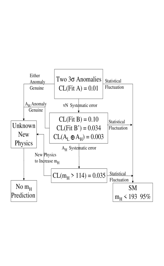
Figure 14: Electroweak schematic diagram.

Taken together the precision electroweak data and the direct searches for the Higgs boson create a complex puzzle with many possible outcomes. An overview is given in the “electroweak schematic diagram,” figure 14. The diagram illustrates how various hypotheses about the two $3\sigma$ anomalies lead to new physics or to the conventional SM fit. The principal conclusion of this paper is reflected in the fact that the only lines leading into the ‘SM’ box are labeled ‘Statistical Fluctuation.’ That is, systematic error alone cannot save the SM fit, since it implies the conflict with the search limit, indicated by the box labeled $CL(m_{H}>114)=0.035$, which in turn either implies new physics or itself reflects statistical fluctuation. This is a consequence of the fact that the combined probability $P_{C}$ defined in equation (1.1) is poor whether the anomalous measurements are included in the fit or not, as summarized in table 5.2.

The ‘New Physics’ box in figure 14 is reached if either $3\sigma$ anomaly is genuine or, conversely, if neither is genuine and the resulting 96.5% $CL$ conflict with the search limit is genuine. It is also possible to invoke statistical fluctuation as the exit line from any of the three central boxes. However we have argued that the global confidence levels indicated for fits A and B are fair reflections of the probability that those fits are fluctuations from the Standard Model. As such they do not favor the SM while they also do not exclude it definitively: “It is a part of probability that many improbable things will happen.”[34]

The smoothest path to the SM might be the one which traverses the central box, fit B, and then exits via ‘Statistical Fluctuation’ to the SM. In this scenario nucleon structure effects might explain the NuTeV anomaly and the 10% confidence level of fit B could be a fluctuation. This is a valid possibility, but two other problems indicated in the central box should also be considered in evaluating this scenario. First, the consistency of the $m_{H}$-sensitive measurements is even more marginal, indicated by the 3.4% confidence level of fit B^′. Second, the troubling $3\sigma$ conflict ($CL=0.003$) between the leptonic and hadronic asymmetry measurements is at the heart of the determination of $m_{H}$. Thus even if we assume that the marginal $CL$ of the global fit is due to statistical fluctuation, the reliability of the prediction of $m_{H}$ hangs on even less probable fluctuations. As noted above, to be consistent with the search limit statistical fluctuations must involve both the ‘anomalous’ hadronic asymmetry measurements and the measurements that conform to the SM fit, especially the leptonic asymmetry measurements and the $W$ boson mass measurement. The conflict with the search limit would be greatly exacerbated if the true value of $x_{W}^{l}[A_{H}]$ were equal to the present value of $x_{W}^{l}[A_{L}]$.

Since there are still some ongoing analyses of the hadronic asymmetry data, there may yet be changes in the final results, but unless major new systematic effects are uncovered the changes are not likely to be large. More precise measurements might be made eventually at a second generation Z factory, such as the proposed Giga-Z project. However, to fully exploit the potential of such a facility it will be necessary to improve the present precision of $\Delta\alpha_{5}(m_{Z})$ by a factor of $\sim 5$ or better, requiring a dedicated program to improve our knowledge of $\sigma(e^{+}e^{-}\rightarrow{\rm HADRONS})$ below $\sim 5$ GeV.[35] The $W$ boson and top quark mass measurements will be improved at Run II of the TeVatron, at the LHC, and eventually at a linear $e^{+}e^{-}$ collider. For instance, an upward shift of the top quark mass[36] or a downward shift of the $W$ boson mass could diminish the inconsistency between the Minimal Data Set and the search limit, while shifts in the opposite directions would increase the conflict.

The issues raised by the current data set heighten the excitement of this moment in high energy physics. The end of the decade of precision electroweak measurements leaves us with a great puzzle, that puts into question the mass scale at which the physics of electroweak symmetry breaking will be found. The solution of the puzzle could emerge in Run II at the TeVatron. If it is not found there it is very likely to emerge at the LHC, which at its design luminosity will be able to search for the new quanta of the symmetry breaking sector over the full range allowed by unitarity.

Acknowledgements: I am grateful to Martin Grunewald for his kind and prompt responses to my questions about the EWWG SM fits. I also thank Kevin McFarland and Geralyn Zeller for useful correspondence and comments. I thank Dimitri Bardin and Giampiero Passarino for kindly verifying the peculiar dependence of $m_{H}$ on $\Gamma_{Z}$, Robert Cahn for classical references, and Max Chanowitz for preparing figure 14.

Table 2.1. SM All-data fit (fit A). Experimental values for the model-independent parameters $g_{L}^{2}[\stackrel{{\scriptstyle(-)}}{{\nu}}N]$ and $g_{R}^{2}[\stackrel{{\scriptstyle(-)}}{{\nu}}N]$ are given for completeness but are not used in the SM fit.

Table 2.2. Evolution of the electroweak data. As noted in the text, the same data is tracked for the three data sets though, following [1], it is grouped into fewer degrees of freedom in the Spring ’02 data set.

	Summer ’98	Spring ’01	Spring ’02
$x_{W}^{l}[A_{L}]$	0.23128 (22)	0.23114 (20)	0.23113 (21)
$x_{W}^{l}[A_{h}]$	0.23222 (33)	0.23240 (29)	0.23220 (29)
$CL(A_{L}\oplus A_{H})$	0.02	0.0003	0.003
$CL(x_{W}^{l})$	0.25	0.02	0.06
$m_{W}$	80.410 (90)	80.448 (34)	80.451 (33)
$\chi^{2}/N$ (no $x_{W}^{\rm OS}[\stackrel{{\scriptstyle(-)}}{{\nu}}N]$	13.8/14	24.6/14	18.4/12
$CL[\chi^{2}/N]$	0.46	0.04	0.10
$x_{W}^{\rm OS}[\stackrel{{\scriptstyle(-)}}{{\nu}}N]$	0.2254 (21)	0.2255 (21)	0.2277 (16)
Pull($x_{W}^{\rm OS}[\stackrel{{\scriptstyle(-)}}{{\nu}}N]$)	1.1	1.2	3.0
$\chi^{2}/N$	15/15	26/15	27.7/13
$CL[\chi^{2}/N]$	0.45	0.04	0.01

Table 2.3. “What if?”: role of $m_{W}$ in shaping the global fit. The first column reflects actual current data with $x_{W}^{\rm OS}[\stackrel{{\scriptstyle(-)}}{{\nu}}N]$ omitted. In the second and third columns $m_{W}$ is assigned hypothetical values as described in the text, while other measurements are held at their Spring ’02 values. In each case the effect of omitting $A_{FB}^{b}$ or $A_{LR}$ is also shown.

Table 3.1. Results for global fits A - D and for the corresponding fits restricted to $m_{H}$-sensitive observables, A^′ - D^′.

Table 3.2. SM fit D, to Minimal Data Set, with $x_{W}^{\rm OS}[\stackrel{{\scriptstyle(-)}}{{\nu}}N]$ and three hadronic asymmetry measurements excluded.

Table 5.1. Predictions for $m_{H}$ from various restricted sets of $m_{H}$-sensitive observables. The value of $m_{H}$ at the $\chi^{2}$ minimum is shown along with the symmetric 90% confidence interval and the likelihood for $m_{H}>114$ GeV. Values indicated as $10-$ or $3000+$ fall below or above the interval $10<m_{H}<3000$ GeV within which the fits are performed.

Table 5.2. Confidence levels and Higgs boson mass predictions for global fits A - D. Each entry shows the value of $m_{H}$ at the $\chi^{2}$ minimum, the symmetric 90% confidence interval, the $\chi^{2}$ confidence level, the confidence level for consistency with the search limit, and the combined likelihood $P_{C}$ from equation (1.1).

Table 7.1 Coefficients for the oblique corrections as defined in equation (7.1).

Figure 1: $\chi^{2}$ distributions as a function of $m_{H}$ from the leptonic asymmetry measurements. The dashed, dot-dashed, and dotted lines are obtained from $A_{LR}$, $A_{FB}^{l}$, and $A_{e,\tau}$ respectively. The solid line is the combined fit to the three asymmetries.

Figure 2: $\chi^{2}$ distributions from the hadronic asymmetry measurements. The dashed, dot-dashed, and dotted lines are obtained from $A_{FB}^{b}$, $A_{FB}^{c}$, and $Q_{FB}$ respectively. The solid line is the combined fit to the three asymmetries.

Figure 3: $\chi^{2}$ distributions from the leptonic (left) and hadronic (right) asymmetry measurements. The dot-dashed lines indicate the respective symmetric 90% $CL$ intervals.

Figure 4: $\chi^{2}$ distributions from non-asymmetry measurements. The dashed, dot-dashed, and dotted lines are obtained from $m_{W}$, $\Gamma_{Z}$, and $R_{l}$ respectively. The solid line is the combined fit to the three measurementss. The dot-dashed lines mark the 95% $CL$ upper limits for the combined distribution and for the distribution obtained from $m_{W}$ alone.

Figure 5: $\chi^{2}$ distribution from $\Gamma_{Z}$ with expanded scale.

Figure 6: $\chi^{2}$ distribution from $x_{W}^{\rm OS}[\stackrel{{\scriptstyle(-)}}{{\nu}}N]$.

Figure 7: $\chi^{2}$ distributions from the $m_{H}$-sensitive observables. The distribution on the left is a fit to the D^′ data set, i.e., restricted to the $m_{H}$-sensitive observables $A_{LR}$, $A_{FB}^{l}$, $A_{e,\tau}$, $m_{W}$, $\Gamma_{Z}$, and $R_{l}$. The distribution on the right is a fit to the remaining $m_{H}$-sensitive observables: $A_{FB}^{b}$, $A_{FB}^{c}$, $Q_{FB}$, and $x_{W}^{\rm OS}[\stackrel{{\scriptstyle(-)}}{{\nu}}N]$. The dot-dashed lines indicate the respective symmetric 90% $CL$ intervals.

Figure 8: $\Delta\chi^{2}$ for two SM global fits. The Minimal Data Set, fit D, is on the left and the all-data set, fit A, is on the right. The 90% symmetric confidence intervals are indicated by the horizontal dot-dashed line. The vertical dashed line denotes the 95% $CL$ lower limit on $m_{H}$ from the direct searches.

Figure 9: Differential and integrated likelihood distributions for the Minimal Data Set (set D, solid lines) and the all-data set (set A, dotted lines). The vertical dashed line denotes the 95% $CL$ lower limit on $m_{H}$ from the direct searches, and the horizontal dot-dashed line indicates the 5% likelihood level.

Figure 10: $\chi^{2}$ distributions (solid lines) for the SM and $S,T$ fits to the Minimal Data Set (data set D). The corresponding values of $S$ (dashed line) and $T$ (dot-dashed line) are read to the scale on the right axis.

Figure 11: $\chi^{2}$ distributions (solid lines) for the SM and $T$-only fits to the Minimal Data Set (data set D). $T$ (dot-dashed line) is read to the scale on the right axis.

Figure 12: $\chi^{2}$ distributions (solid lines) for the SM and $S,T$ fits to data set B, i.e., including the hadronic asymmetry measurements but not $x_{W}^{\rm OS}[\stackrel{{\scriptstyle(-)}}{{\nu}}N]$. $S$ (dashed line) and $T$ (dot-dashed line) are read to the scale on the right axis.

Figure 13: $\chi^{2}$ distributions (solid lines) for $S,T$ fits to the all-data set, data set A. The distribution for $S=T=0$ is not equivalent to the SM fit since it uses the model-independent NuTeV fit to $g_{L,R}$ as discussed in the text. $S$ (dashed line) and $T$ (dot-dashed line) are read to the scale on the right axis.

References

- [1] The LEP Collaborations ALEPH, DELPHI, L3, OPAL, the LEP Electroweak Working Group, and the SLD Heavy Flavour and Electroweak Groups, LEPEWWG/2002-01, May 8, 2002.
- [2] LEP Higgs working group, CERN-EP/2001-055.
- [3] M.S. Chanowitz, Phys. Rev. D59:073005,1999, e-Print hep-ph/9807452.
- [4] The LEP Collaborations ALEPH, DELPHI, L3, OPAL, the LEP Electroweak Working Group, and the SLD Heavy Flavour and Electroweak Groups, CERN-EP/99-15, February 8, 1999.
- [5] The LEP Collaborations ALEPH, DELPHI, L3, OPAL, the LEP Electroweak Working Group, and the SLD Heavy Flavour and Electroweak Groups, LEPEWWG/2001-01, May 31, 2001.
- [6] G.P. Zeller, K.S. McFarland et al., Phys. Rev. Lett. 88:091802, 2002.
- [7] M.E. Peskin, T. Takeuchi (SLAC), Phys. Rev. D46:381,1992.
- [8] M.S. Chanowitz, M.K. Gaillard, Nucl. Phys. B261:379,1985; M.S. Chanowitz, Presented at Zuoz Summer School on Hidden Symmetries and Higgs Phenomena, Zuoz, Switzerland, Aug 1998, in Zuoz 1998, Hidden symmetries and Higgs phenomena, ed. D. Graudenz, PSI Proceeedings 98-02, and e-Print: hep-ph/9812215.
- [9] M.S. Chanowitz, W.Kilgore, Phys. Lett. B322:147,1994, and e-Print: hep-ph/9311336; ibid, B347:387,1995, and e-Print: hep-ph/9412275; J. Bagger et al., Phys. Rev. D52:3878,1995, and e-Print: hep-ph/9504426.
- [10] M.S. Chanowitz, Phys. Rev. Lett. 87:231802, 2001, e-Print: hep-ph/0104024.
- [11] S. Davidson, S. Forte, P. Gambino, N. Rius, A. Strumia, JHEP 0202:037,2002, e-Print: hep-ph/0112302.
- [12] G. Altarelli, N. Di Bartolomeo, F. Feruglio, R. Gatto, M.L. Mangano, Phys. Lett. B375:292,1996 and e-Print: hep-ph/9601324; P. Chiappetta, J. Layssac, F.M. Renard, Phys. Rev. D54:789,1996, e-Print: hep-ph/9601306; K.S. Babu, C.F. Kolda, John March-Russell, Phys. Rev. D54:4635,1996, e-Print: hep-ph/9603212; K. Agashe, M. Graesser, I. Hinchliffe, M. Suzuki, Phys .Lett. B385:218,1996, e-Print: hep-ph/9604266.
- [13] X-G. He and G. Valencia, e-Print: hep-ph/0203036, Mar. 2002.
- [14] C.T. Hill, Phys. Lett. B266:419,1991; Phys. Lett. B345:483,1995.
- [15] D. Choudhury, T.M.P. Tait, C.E.M. Wagner, Phys. Rev. D65:053002,2002, e-Print: hep-ph/0109097.
- [16] D. Chang, W-F. Chang, E Ma, Phys. Rev. D61:037301,2000, e-Print: hep-ph/9909537.
- [17] G.P. Zeller, K.S. McFarland et al., Phys. Rev. D65:111103,2002, e-Print: hep-ex/0203004.
- [18] E. Sather, Phys. Lett. B274:433,1992; E.N. Rodianov, A.W. Thomas, J.T. Londergan, Mod. Phys. Lett. A9:1799, 1994; F. Cao and A.I. Signal, Phys. ReV C62: 015203, 2000.
- [19] M. Elsing, presented at XXXVII Rencontres de Moriond, Electroweak Interactions and Unified Theories, Les Arcs, March 9-16-2002 (posted at http://moriond.in2p3.fr/EW/2002/transparencies).
- [20] D. Bardin et al., Comput. Phys. Commun.133:229,2001, e-Print hep-ph/9908433.
- [21] H. Burkhardt and B. Pietrzyk, LAPP-EXP-2001-03, Feb 2001 (submitted to Phys. Lett. B).
- [22] V.A. Dzuba, V.V. Flambaum, J.S.M. Ginges, Apr 2002, e-Print: hep-ph/0204134.
- [23] G. Montagna, O. Nicrosini, F. Piccinini, G. Passarino, Comput. Phys. Commun. 117:278-289,1999, e-Print: hep-ph/9804211.
- [24] A. Ferroglia, G. Ossola, M. Passera, A. Sirlin, Phys. Rev. D65:113002,2002, e-Print: hep-ph/020322.
- [25] G. Altarelli, F. Caravaglios, G.F. Giudice, P. Gambino, G. Ridolfi, JHEP 0106:018,2001, e-Print: hep-ph/0106029.
- [26] V.A. Novikov, L.B. Okun, A.N. Rozanov, M.I. Vysotsky, e-Print: hep-ph/0203132, Mar. 2002; and Phys. Lett. B529:111-116,2002, e-Print: hep-ph/0111028.
- [27] D.C. Kennedy and B.W. Lynn, Nucl. Phys. B322:1,1989.
- [28] B. Holdom, Phys. Lett. B259:329-334,1991.
- [29] L.J. Hall, C.F. Kolda, Phys.Lett.B459:213,1999, e-Print: hep-ph/9904236; J.A. Bagger, A.F. Falk, M. Swartz, Phys. Rev. Lett. 84:1385,2000, e-Print: hep-ph/9908327; R.S. Chivukula, N. Evans, Phys. Lett. B464:244,1999, e-Print: hep-ph/9907414; M.E. Peskin, J.D. Wells, Phys. Rev. D64:093003,2001 and e-Print: hep-ph/0101342.
- [30] R. Dashen and H. Neuberger, Phys.Rev.Lett.50:1897,1983.
- [31] See for instance M. Lüscher and P. Weisz, Nucl. Phys.B318:705,1989; J. Kuti, L. Lin, and Y. Shen, Phys.Rev.Lett.61:678,1988; A. Hasenfratz et al., Nucl. Phys.B317:81,1989; G.R. Bhanot and K. Bitar, Phys.Rev.Lett.61:798,1988.
- [32] M.S. Chanowitz, Phys. Rev. D63:076002,2001, e-Print: hep-ph/0010310. A lattice calculation with compatible results, though with a different purpose, is reported in U. Heller, M. Klomfass, H. Neuberger, and P. Vranas, Nucl. Phys. B405:555,1993, e-Print: hep-ph/9303215.
- [33] C. Csaki, J. Erlich, John Terning, e-Print: hep-ph/0203034, Mar. 2002; B. Dobrescu and J. Terning, Phys. Lett. B416:129,1998, e-Print: hep-ph/9709297. For a review with citations of additional examples see C. T. Hill and E. H. Simmons, FERMILAB-PUB-02-045-T, BUHEP-01-09, Mar 2002, submitted to Phys.Rep., e-Print: hep-ph/0203079.
- [34] Agathon, quoted by Aristotle in the Poetics.
- [35] F. Jegerlehner, DESY-01-028, Mar 2001, e-Print: hep-ph/0104304.
- [36] T. Aziz, A. Gurtu, CERN-OPEN-2001-067, Aug 2001, Submitted to Phys. Lett. B, e-Print: hep-ph/0110177.