GPDs, form factors and Compton scattering

Abstract

The basic theoretical ideas of the handbag factorization and its application to wide-angle scattering reactions are reviewed. With regard to the present experimental program carried out at JLab, wide-angle Compton scattering is discussed in some detail.

1 Introduction

As is well-known factorization is an important property of QCD whithout which we would not be able to calculate form factors or cross sections. Factorization into a hard parton-level subprocess to be calculated from perturbative QED and/or QCD, and soft hadronic matrix elements which are subject to non-perturbative QCD and are not calculable at present, has been shown to hold for a number of reactions provided a large scale, i.e. a large momentum transfer, is available. For other reactions factorization is a reasonable hypothesis. In the absence of a large scale we don’t know how to apply QCD and, for the interpretation of scattering reactions, we have to rely upon effective theories or phenomenological models as for instance the Regge pole one.

For hard exclusive processes there are two different factorization schemes available. One of the schemes is the handbag factorization (see Fig. 1) where only one parton participates in the hard subprocess (e.g. $\gamma q\to\gamma q$ in Compton scattering) and the soft physics is encoded in generalized parton distributions (GPDs) [1, 2]. The handbag approach applies to deep virtual exclusive scattering (e.g. DVCS) where one of the photons has a large virtuality, $Q^{2}$, while the squared invariant momentum transfer, $-t$, from the ingoing hadron to the outgoing one is small. It also applies to wide-angle scattering (WACS) where $Q^{2}$ is small while $-t$ (and $-u$) are large [3, 4]. This class of reactions is the subject of my talk. For wide-angle scattering there is an alternative scheme, the leading-twist factorization [5]. Here all valence quarks the involved hadrons are made off participate in the hard scattering (e.g. $\gamma qqq\to\gamma qqq$ in Compton scattering) while the soft physics is encoded in distribution amplitudes representing the probability amplitudes for finding quarks in a hadron with a given momentum distribution (see Fig. 1).

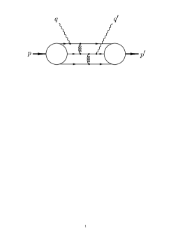
Figure 1: Handbag (left) and leading-twist (right) factorization for Compton scattering.

Since neither the GPDs nor the distribution amplitudes can be calculated whithin QCD at present, it is difficult to decide which of the factorization schemes provides an appropriate description of, say, wide-angle Compton scattering at $-t\simeq 10~{}{\rm GeV}^{2}$. The leading-twist factorization probably requires larger $-t$ than the handbag one since more details of the hadrons have to be resolved. Recent phenomenological and theoretical developments [6] support this conjecture. In the following I will discuss the handbag contribution only, assuming that the leading-twist one is negligibly small for momentum transfers of about $10~{}{\rm GeV}^{2}$. The ultimate decision whether or not this assumption is correct, is to be made by experiment.

It should be noted that immediately after the discovery of the partons in the late sixties constituent scattering models had been invented [7, 8] which bear resemblance to the handbag contribution. As compared to these early attempts the handbag factorization has now a sound theoretical foundation. Particularly the invention of GPDs effectuated a decisive step towards a theoretical understanding of hard exclusive reactions.

2 The handbag in wide-angle Compton scattering

In 1998 Radyushkin [3] calculated the handbag contribution to Compton scattering starting from double distributions. Somewhat later Diehl, Feldmann, Jakob and myself calculated it on the basis of parton ideas [4]. Both approaches arrived at essentially the same results. Here, I will briefly describe our approach because I am more familiar with it. Our kinematical requirements are that the three Mandelstam variables $s,\,-t,\,-u$ are much larger than $\Lambda^{2}$ where $\Lambda$ is a typical hadronic scale of order $1\,~{}{\rm GeV}$. The bubble in the handbag is viewed as a sum over all possible parton configurations as in deep ineleastic lepton-proton scattering (DIS). The contribution we calculate is defined by the requirement of restricted parton virtualities, $k_{i}^{2}<\Lambda^{2}$, and intrinsic transverse parton momenta, ${\bf k_{\perp i}}$, which satisfy $k_{\perp i}^{2}/x_{i}<\Lambda^{2}$, where $x_{i}$ is the momentum fraction parton $i$ carries.

It is of advantage to work in a symmetrical frame which is a c.m.s rotated in such a way that the momenta of the incoming ($p$) and outgoing ($p^{\prime}$) proton momenta have the same light-cone plus components. In this frame the skewness, defined as

$$\xi=\frac{(p-p^{\prime})^{+}}{(p+p^{\prime})^{+}}\,,$$ (1)

is zero. One can then show that the subprocess Mandelstam variables $\hat{s}$ and $\hat{u}$ are the same as the ones for the full process, Compton scattering off protons, up to corrections of order $\Lambda^{2}/t$:

$$\hat{s}=(k_{j}+q)^{2}\simeq(p+q)^{2}=s\,,\quad\hat{u}=(k_{j}-q^{\prime})^{2}\simeq(p-q^{\prime})^{2}=u\,.$$ (2)

The active partons, i.e. the ones to which the photons couple, are approximately on-shell, move collinear with their parent hadrons and carry a momentum fraction close to unity, $x_{j},x_{j}^{\prime}\simeq 1$. Thus, like in DVCS, the physical situation is that of a hard parton-level subprocess, $\gamma q\to\gamma q$, and a soft emission and reabsorption of quarks from the proton. The helicity amplitudes for WACS then read

$${M}_{\mu^{\prime}+,\,\mu+}(s,t) = \;2\pi\alpha_{\rm elm}\left[{T}_{\mu^{\prime}+,\,\mu+}(s,t)\,(R_{V}(t)+R_{A}(t))\,\right.$$ (3)

$$\quad\left.+\,{T}_{\mu^{\prime}-,\,\mu-}(s,t)\,(R_{V}(t)-R_{A}(t))\right]\,,$$

$${M}_{\mu^{\prime}-,\,\mu+}(s,t) = \;-\pi\alpha_{\rm elm}\frac{\sqrt{-t}}{m}\left[T_{\mu^{\prime}+,\,\mu+}(s,t)\,+\,{T}_{\mu^{\prime}-,\,\mu-}(s,t)\,\right]\,R_{T}(t)\,.$$

$\mu,\,\mu^{\prime}$ denote the helicities of the incoming and outgoing photons, respectively. The helicities of the protons in ${M}$ and quarks in the hard scattering amplitude $T$ are labeled by their signs. The hard scattering has been calculated to next-to-leading order perturbative QCD [9], see Fig. 2. To this order the gluonic subprocess, $\gamma g\to\gamma g$ has to be taken into account as well. The form factors $R_{i}$ represent $1/x$-moments of GPDs at zero skewness.

Figure 2: Sample Feynman graphs for $\gamma q\to\gamma q$ to NLO in perturbative QCD.

$R_{T}$ controls the proton helicity flip amplitude while the combination $R_{V}+R_{A}$ is the response of the proton to the emission and reabsorption of quarks with the same helicity as it and $R_{V}-R_{A}$ that one for opposite helicities. The identification of the form factors with $1/x$-moments of GPDs is possible because the plus components of the proton matrix elements dominate as in DIS and DVCS. This is non-trivial feature given that, in contrast to DIS and DVCS, not only the plus components of the proton momenta but also their minus and transverse components are large here. A more technical aspect is the fact that the handbag approach naturally demands the use of light-cone techniques. Thus, (3) is a light-cone helicity amplitude. To facilitate comparison with experiment one may transform the amplitudes (3) to the ordinary c.m.s. helicity basis [9, 10].

3 Modeling the GPDs

The structure of the handbag amplitude, namely its representation as a product of perturbatively calculable hard scattering amplitudes and $t$-dependent form factors

$${M}(s,t)\sim{T}(s,t)\,R(t)$$ (4)

is the essential result. Refuting the handbag approach necessitates experimental evidence against the structure (4). In oder to make actual predictions for Compton scattering however models for the soft form factors or rather for the underlying GPDs are required. A first attempt to parameterize the GPDs $H$ and $\widetilde{H}$ at zero skewness reads [3, 4, 9, 11] (see also [12, 13])

$$H^{a}(\bar{x},0;t) = \exp{\left[a^{2}t\frac{1-\bar{x}}{2\bar{x}}\right]}\,q_{a}(\bar{x})\,,$$

$$\widetilde{H}^{a}(\bar{x},0;t) = \exp{\left[a^{2}t\frac{1-\bar{x}}{2\bar{x}}\right]}\,\Delta q_{a}(\bar{x})\,,$$ (5)

where $q(x)$ and $\Delta q(x)$ are the usual unpolarized and polarized parton distributions in the proton. $a$, the transverse size of the proton, is the only free parameter and even it is restricted to the range of about 0.8 to 1.2 $~{}{\rm GeV}^{-1}$ for a realistic proton. Note that $a$ mainly refers to the lowest Fock states of the proton which, as phenomenological experience tells us, are rather compact. The model (5) is designed for large $-t$. Hence, forced by the Gaussian in (5), large $x$ is implied, too. Despite of this the normalization of the model GPDs at $t=0$ is correct.

The model (5) can be motivated by overlaps of light-cone wave functions. As has been shown [4, 14, 15] GPDs possess a representation in terms of such overlaps. Assuming a Gaussian $k_{\perp}$ dependence for the $N$-particle Fock state wave function

$$\Psi_{N}=\Phi_{N}(x_{1},\cdots x_{N})\,\exp{\left[-a_{N}^{2}\sum_{i=1}^{N}k_{\perp i}^{2}/x_{i}\right]}\,,$$ (6)

which is in line with the central assumption of the handbag approach of restricted $k_{\perp i}^{2}/x_{i}$, necessary to achieve factorization of the amplitudes into soft and hard parts, and assuming further $a_{N}=a$ for all $N$ in order to simplify matters, each overlap provides the Gaussian appearing in (5). The remainder of the overlaps summed over all $N$ is just the Fock state representation of the parton distribution [5]. Thus, there is no need to specify the full $x$ dependence of the light-cone wave function in order to arrive at (5). Note that $\Phi_{N}$ may depend on quark masses.

The simple model (5) may be improved in various ways. For instance, one may treat the lowest Fock states explicitly [4], take into account the evolution of the GPDs [16] or improve the parameterization in such a way that it also holds for small $x$ [17]. One may also consider wave function with a power-law dependence on ${\bf k}_{\perp}$ instead of the Gaussian in (6) [18].

From the GPDs one can calculate the various form factors by taking appropriate moments, e.g.

$$F_{1}=\sum_{q}e_{q}\int_{-1}^{1}d\bar{x}H^{q}(\bar{x},0;t)\,,\quad R_{V}=\sum_{q}e_{q}^{2}\int_{-1}^{1}\frac{d\bar{x}}{\bar{x}}H^{q}(\bar{x},0;t)\,.$$ (7)

Results for the form factors are shown in Fig. 3. Obviously, as the comparison with experiment [19] reveals the model GPDs work quite well in the case of the Dirac form factor [4]. The scaled form factors $t^{2}F_{1}$ and $t^{2}R_{i}$ exhibit broad maxima which mimick dimensional counting in a range of $-t$ from, say, $3$ to about $20\,~{}{\rm GeV}^{2}$. For very large values of $-t$, well above $100\,~{}{\rm GeV}^{2}$, the form factors turn gradually into a $\propto 1/t^{4}$ behaviour; this is the region where the leading-twist contribution takes the lead. The position of the maximum of a scaled form factor is approximately located at

$$t_{0}\simeq-4a^{-2}\,\left\langle\frac{1-x}{x}\right\rangle^{-1}_{F(R)}\,.$$ (8)

The mildly $t$-dependent mean value $\langle(1-x)/x\rangle$ has a value of about $1/2$.

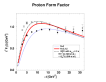
Figure 3: Predictions for the Dirac form factor of the proton (left) and for the Compton form factors (right)[4]. Data are taken from Ref. [19].

The Pauli form factor $F_{2}$ and its Compton analogue $R_{T}$ contribute to proton helicity flip matrix elements and are related to the GPD $E$

$$F_{2}=\sum_{q}e_{q}\int_{-1}^{1}d\bar{x}E^{q}(\bar{x},0;t)\,,\quad R_{T}=\sum_{q}e_{q}^{2}\int_{-1}^{1}\frac{d\bar{x}}{\bar{x}}E^{q}(\bar{x},0;t)\,.$$ (9)

The overlap representation of $E$ [14] involves components of the proton wave functions where the parton helicities do not sum up to the helicity of the proton. In other words, parton configurations with non-zero orbital angular momentum contribute to it. A simple ansatz for a proton valence Fock state wave function that involves orbital angular momentum is

$$\Psi_{3}^{-}\sim\sum\frac{{\bf k}_{\perp i}}{\sqrt{x_{i}}}\exp{[-a_{-}^{2}\sum{k^{2}_{\perp i}}/{x_{i}}]}\,.$$ (10)

Evaluating the overlap contributions to $F_{2}$ and $R_{T}$ from this wave function and from (6), one finds

$$R_{T}/R_{V}\,,\;\;F_{2}/F_{1}\,\propto m/\sqrt{-t}$$ (11)

rather than $\propto m^{2}/t$. (11) is in agreement with the recent JLab measurement [20] while the SLAC data [21] are rather compatible with a $\propto m^{2}/t$ behaviour. The new experimental results on $F_{2}/F_{1}$ have been discussed in the same spirit as here in Ref. [22]. Clearly, more phenomenological work on $E$, $F_{2}$ and $R_{T}$ is needed.

For an estimate of the size of $R_{T}$ one may simply assume that $R_{T}/R_{V}$ roughly behaves as its electromagnetic counter part $F_{2}/F_{1}$. Hence,

$$\kappa_{T}=\frac{\sqrt{-t}}{2m}\frac{R_{T}}{R_{V}}\simeq\frac{\sqrt{-t}}{2m}\frac{F_{2}}{F_{1}}$$ (12)

has a value of 0.37 [20].

4 Results for Compton scattering

I am now ready to discuss results for Compton scattering. The cross section reads

$$\frac{d\sigma}{dt} = \frac{d\hat{\sigma}}{dt}\left\{\frac{1}{2}[R_{V}^{2}(t)(1+\kappa_{T}^{2})+R_{A}^{2}(t)]\right.$$ (13)

$$\left.\quad-\frac{us}{s^{2}+u^{2}}[R_{V}^{2}(t)(1+\kappa_{T}^{2})-R_{A}^{2}(t)]\right\}+O(\alpha_{s})\,,$$

where $d\hat{\sigma}/dt$ is the Klein-Nishina cross section for Compton scattering of point-like spin-1/2 particles. This cross section is multiplied by a factor that describes the structure of the proton in terms of the three form factors. The predictions from the handbag are in fair agreement with experiment [23], see Fig. 4. The approximative $s^{6}$-scaling behaviour is related to the broad maximum at about $8~{}{\rm GeV}^{2}$ the form factors exhibit, see (8). Clearly, more accurate date are needed for a detailed comparison. The JLab will provide such data soon.

Figure 4: Predictions for the Compton cross section (left) and for the helicity correlation $A_{LL}$ (right). NLO corrections and the tensor form factor are taken into account (scenario A) [9], in scenario B they are neglected. Data are taken from Ref. [23].

Another interesting observable for Compton scattering is the helicity correlation, $A_{LL}$, between the initial state photon and proton or, equivalently, the helicity transfer, $K_{LL}$, from the incoming photon to the outgoing proton. From the handbag approach one obtains [9, 24]

$$A_{LL}=K_{LL}\simeq\hat{A}_{LL}\frac{R_{A}}{R_{V}}+O(\kappa_{T},\alpha_{s},\beta)\,,$$ (14)

where $\hat{A}_{LL}$ is the corresponding observable for $\gamma q\to\gamma q$

$$\hat{A}_{LL}=\frac{s^{2}-u^{2}}{s^{2}+u^{2}}\,.$$ (15)

The subprocess observable is diluted by the ratio of the form factors $R_{A}$ and $R_{V}$ as well as by other corrections but its shape essentially remains unchanged. The predictions for $A_{LL}$ from the leading-twist approach drastically differ from the ones shown in Fig. 4. For $\theta\raisebox{-4.0pt}{$\,\stackrel{{\scriptstyle\textstyle<}}{{\sim}}\,$}110^{\circ}$ negative values for $A_{LL}$ are obtained for all but one examples of distribution amplitudes. The diquark model[26], a variant of the leading-twist approach, also leads to a negative value for $A_{LL}$. The JLab E99-114 collaboration [27] has presented a first measurement of $A_{LL}$ at a c.m.s. scattering angle of $120^{\circ}$ and a photon energy of $4.3~{}{\rm GeV}$. This still preliminary data point is in agreement with the prediction from the handbag, the leading-twist calculations fails badly. A measurement of the angular dependence of $A_{LL}$ would be highly welcome for establishing the handbag approach . For predictions of other polarization observables for Compton scattering I refer to Refs. [9, 24].

5 Other applications of the handbag mechanism

The handbag approach has been applied to several other high-energy wide-angle reactions. Thus, as shown in Ref. [24], the calculation of real Compton scattering can be straightforwardly extended to virtual Compton scattering provided $Q^{2}/-t\ll 1$. Elastic hadron-hadron scattering can be treated as well [24]. Details have not yet been worked out but it has been shown that form factors of the type discussed in Sect. 3 control elastic scattering, too. The experimentally observed scaling behaviour of these cross sections can be attributed to the broad maximum the scaled form factors show, see Fig. 3.

The time-like processes two-photon annihilations into pairs of mesons or baryons can also be calculated, the arguments for handbag factorization hold here as well as has recently been shown in Refs. [29, 30], see also the talk by Weiss [31]. The cross section for the production of baryon pairs read

$$\frac{d\sigma}{dt}\,(\,\gamma\gamma\,\to\,\,B\overline{B}\,) = \frac{4\pi\alpha^{2}_{\rm elm}}{s^{2}\sin^{2}\theta}\Big{\{}\big{|}R_{A}^{B}(s)+R_{P}^{B}(s)\big{|}^{2}$$ (16)

$$+ \cos^{2}\theta\,\big{|}R_{V}^{B}(s)\big{|}^{2}\,+\,\frac{s}{4m^{2}}\,\big{|}R_{P}^{B}(s)\big{|}^{2}\Big{\}}\,.$$

The form factors represent integrated $B\overline{B}$ distribution amplitudes $\Phi_{B\overline{B}\,i}$ which are time-like versions of GPDs at a time-like skewness of $1/2$. They read ($i=V,\,A,\,P$)

$$R^{B}_{i}(s)\,=\,\sum_{q}\,e_{q}^{2}\,F_{i}^{Bq}(s)\,,\hskip 28.45274ptF_{i}^{Bq}(s)=\int_{0}^{1}dz\,\Phi^{q}_{B\overline{B}\,i}(z,\zeta=1/2,s)\,.$$ (17)

The form factors have not been modeled by us, they are extracted from the measured intergrated cross sections. The result for the effective form factor for $\gamma\gamma\to p\overline{p}$, being a combination of the dominant axial vector form factor and the pseudoscalar one, is shown in Fig. 5. The form factors behave similar to the magnetic one, $G_{M}(s)$, in the time-like region and have the same size as it within about a factor of two [34].

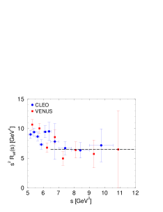
Figure 5: The scaled annihilation form factor $s^{2}|R_{A}^{p}|$ as extracted from the data of Refs. [32, 33]. The dashed line represents a fit to the data above $6.5\,~{}{\rm GeV}\,^{2}$.

A characterisic feature of the handbag is the $q\overline{q}$ intermediate state implying the absence of isospin-two components in the final state. A consequence of this property is

$$\frac{d\sigma}{dt}(\gamma\gamma\to\pi^{0}\pi^{0})=\frac{d\sigma}{dt}(\gamma\gamma\to\pi^{+}\pi^{-})\,,$$ (18)

which is independent of the soft physics input and is, in so far, a hard prediction of the handbag approach. The absence of the isospin-two components combined with flavor symmetry allows one to calculate the cross section for other $B\overline{B}$ channels using the form factors for $p\overline{p}$ as the only soft physics input. It is important to note that the leading-twist mechanism has difficulties to account for the size of the cross sections [35] while the diquark model [36] is in fair agreement with experiment for $\gamma\gamma\to B\overline{B}$.

Photo- and electroproduction of mesons have also been discussed within the handbag approach [11] using, as in deep virtual electroproduction [37], a leading-twist mechanism for the generation of the meson. It turns out, however, that the photoproduction cross section is way below experiment. The reason for this failure is not yet understood. Either the vector meson dominance contribution is still large or the leading-twist generation of the meson underestimates the handbag contribution. Despite of this the handbag contribution to photo-and electroproduction has several interesting properties which perhaps survive an improvement of the approach. For instance, the helicity correlation $\hat{A}_{LL}$ for the subprocess $\gamma q\to\pi q$ is the same as for $\gamma q\to\gamma q$, see (15). $A_{LL}$ for the full process is diluted by form factors similar to the case of Compton scattering. Another result is the ratio of the production of $\pi^{+}$ and $\pi^{-}$ which is approximately given by

$$\frac{d\sigma(\gamma n\to\pi^{-}p)}{d\sigma(\gamma p\to\pi^{+}n)}\simeq\left[\frac{e_{d}u+e_{u}s}{e_{u}u+e_{d}s}\right]^{2}\,.$$ (19)

6 Summary

I have reviewed the theoretical activties on applications of the handbag mechanism to wide-angle scattering. There are many interesting predictions still awaiting their experimental examination. At this workshop many new, mainly preliminary data for wide-angle scattering from JLab have been presented, more data will come soon. There are first hints that the handbag mechanism plays an important role. However, before we can draw firm conclusions we have to wait till the data have been finalized. For the kinematical situation available at JLab substantial corrections to the handbag contribution are to be expected. This may render a detailed quantitative comparison between theory and experiment difficult.

Acknowledgments. It is a pleasure to thank the organizers of this workshop Carl Carlson, Jean-Marc Laget, Anatoly Radyushkin, Paul Stoler and Bogdan Wojtsekhowski for inviting me to attend this interesting and well organized workshop at Jefferson Lab.

References

- [1] D. Müller, D. Robaschik, B. Geyer, F. M. Dittes and J. Hořejši, Fortsch. Phys. 42, 101 (1994) [hep-ph/9812448].
- [2] A. V. Radyushkin, Phys. Rev. D56 5524 (1997) [hep-ph/9704207]; X. Ji, Phys. Rev. D55 7114 (1997) [hep-ph/9609381].
- [3] A. V. Radyushkin, Phys. Rev. D 58, 114008 (1998) [hep-ph/9803316].
- [4] M. Diehl, T. Feldmann, R. Jakob and P. Kroll, Eur. Phys. J. C 8, 409 (1999) [hep-ph/9811253].
- [5] G. P. Lepage and S. J. Brodsky, Phys. Rev. D 22, 2157 (1980).
- [6] J. Bolz and P. Kroll, Z. Phys. A 356, 327 (1996) [hep-ph/9603289]; V. M. Braun, A. Lenz, N. Mahnke and E. Stein, Phys. Rev. D 65, 074011 (2002) [hep-ph/0112085]; D. Diakonov and V. Y. Petrov, hep-ph/0009006.
- [7] J.D. Bjorken and E.A. Paschos, Phys. Rev. 185, 1975 (1969); D.M. Scott, Phys. Lett. 53B, 185 (1974).
- [8] D. Sivers, S.J. Brodsky and R. Blankenbecler, Phys. Rep. 23 C, 1 (1976) and references therein.
- [9] H. W. Huang, P. Kroll and T. Morii, Eur. Phys. J. C 23, 301 (2002) [hep-ph/0110208].
- [10] M. Diehl, Eur. Phys. J. C 19, 485 (2001) [hep-ph/0101335].
- [11] H. W. Huang and P. Kroll, Eur. Phys. J. C 17, 423 (2000) [hep-ph/0005318].
- [12] A. V. Afanasev, hep-ph/9910565.
- [13] V. Barone et al., Z. Phys. C 58, 541 (1993).
- [14] M. Diehl, T. Feldmann, R. Jakob and P. Kroll, Nucl. Phys. B 596, 33 (2001) [Erratum-ibid. B 605, 647 (2001)] [hep-ph/0009255].
- [15] S. J. Brodsky, M. Diehl and D. S. Hwang, Nucl. Phys. B 596, 99 (2001) [hep-ph/0009254].
- [16] C. Vogt, Phys. Rev. D 63, 034013 (2001) [hep-ph/0007277].
- [17] M. Vanderhaeghen, these proceedings; K. Goeke, . V. Polyakov and M. Vanderhaeghen, Prog. Part. Nucl. Phys. 47, 401 (2001) [hep-ph/0106012].
- [18] A. Mukherjee, I.V. Musatov, H.C. Pauli and A.V. Radyushkin, hep-ph/0205315.
- [19] A.F. Sill et al., Phys. Rev. D48, 29 (1993); A. Lung et al., Phys. Rev. Lett. 70, 718 (1993).
- [20] O. Gayou et al. [Jefferson Lab Hall A Collaboration], Phys. Rev. Lett. 88, 092301 (2002) [nucl-ex/0111010].
- [21] L. Andivahis et al., Phys. Rev. D 50, 5491 (1994).
- [22] J.P. Ralston, P. Jain and R. Buniy, these proceedings and in those of the Conf. of Intersections of Particle and Nuclear Physics, Quebec (2000).
- [23] M.A. Shupe et al., Phys. Rev. D19, 1921 (1979).
- [24] M. Diehl, T. Feldmann, R. Jakob and P. Kroll, Phys. Lett. B 460, 204 (1999) [hep-ph/9903268].
- [25] T. C. Brooks and L. Dixon, Phys. Rev. D 62, 114021 (2000) [hep-ph/0004143].
- [26] P. Kroll, M. Schürmann and W. Schweiger, Intern. J. Mod. Phys. A 6, 4107 (1991).
- [27] A. Nathan, for the E99-114 JLab collaboration, these proceedings
- [28] F. Cano and J. M. Laget, Phys. Rev. D 65, 074022 (2002) [hep-ph/0111146].
- [29] M. Diehl, P. Kroll and C. Vogt, Phys. Lett. B 532, 99 (2002) [hep-ph/0112274; C. Vogt, these proceedings.
- [30] M. Diehl, P. Kroll and C. Vogt, hep-ph/0206288.
- [31] C. Weiss, these proceedings; A. Freund, A. Radyushkin, A. Schäfer and C. Weiss, work in progress.
- [32] M. Artuso et al. [CLEO Collaboration], Phys. Rev. D 50, 5484 (1994).
- [33] H. Hamasaki et al. [VENUS Collaboration], Phys. Lett. B 407, 185 (1997).
- [34] T. A. Armstrong et al. [E760 Collaboration], Phys. Rev. Lett. 70, 1212 (1993).
- [35] G. R. Farrar, E. Maina and F. Neri, Nucl. Phys. B 259, 702 (1985) [Erratum-ibid. B 263, 746 (1985)].
- [36] P. Kroll et al., Phys. Lett. B 316, 546 (1993) [hep-ph/9305251]; C.F. Berger, B. Lechner and W. Schweiger, Fizika B 8, 371 (1999).
- [37] J.C. Collins, L. Frankfurt and M. Strikman, Phys. Rev. D56, 2982 (1997) [hep-ph/9611433]; A. V. Radyushkin, Phys. Lett. B 385, 333 (1996) hep-ph/9605431].