Scattering amplitudes at finite temperature

Abstract

We present a simple set of rules for obtaining the imaginary part of a self energy diagram at finite temperature in terms of diagrams that correspond to physical scattering amplitudes.

I Introduction

In this paper we discuss a set of rules for calculating the imaginary part of self energy diagrams. These rules have a simple diagrammatic representation in terms of scattering amplitudes. They have been deduced by studying a large set of diagrams; a derivation from first principles is in progress and will be presented in another paper.

It is well known that the imaginary part of the retarded self energy is an important quantity in thermal field theory: it provides information about decay and production rates of particles, among other things. The physics that is contained in the imaginary part of the self energy is revealed by writing it as the product of two scattering amplitudes. At the one loop level, the structure of the scattering amplitude has been understood for some time Weld . Extension to higher loops is not straightforward. In this paper we discuss cutting rules in the context of this problem. We show that rules exist that make it easy to understand the physical content of the imaginary part of a self energy diagram at high loop order.

We begin by reviewing some basic concepts and defining some notation:

a) Off shell propagators describe the behaviour of fields that propagate through the medium until they undergo interactions with other fields. Diagrammatically, off shell propagators are represented by continuous lines that begin and end at interaction vertices.

b) On shell propagators carry delta functions of the form $\delta(P^{2}-m^{2})$ where $P$ is the momentum of the field. On shell propagators correspond to fields that do not propagate through the medium.

c) Consider any closed loop in which all of the propagators are off shell and momentum is free to flow around the loop. If any one of the propagators in the loop is put on shell, momentum is no longer free to flow around the loop and the loop is effectively ‘opened.’

d) There are two kinds of propagators that are on shell. We call these two types of propagators “cut” propagators and “tic-ed” propagators. Cut propagators and tic-ed propagators carry different thermal factors. This point will be explained in detail.

e) A “cut line” is a line that divides the self energy into two pieces, each of which has one external leg. Any propagator that is crossed by a cut line is put on shell and becomes a “cut” propagator.

f) Diagrammatically, our notation is as follows. In a self energy diagram, a cut propagator is a propagator that is crossed by the cut line and a tic-ed propagator is drawn with a double tic mark through it. To obtain scattering amplitudes, all on shell propagators (cut or tic-ed) are split into two pieces, each of which has an end that is not connected to a vertex. As a result, the cut line divides the self energy diagram into two separate amplitudes, and (as will be explained below) the tic-ed propagators cause each amplitude to have the form of a tree amplitude, with no closed loops. The lines obtained from the splitting of on shell propagators represent the emission or absorption of fields by the medium. The lines that represent absorbed fields are drawn slanting backwards from the vertex and lines that represent emitted particles slanting forward from the vertex.

g) For any given diagram, the number of $\delta$ functions, or the number of on shell = (cut + tic-ed) propagators, is equal to $L+1$ where $L$ is the number of loops.

To begin, we consider a one loop calculation. Following Weldon Weld we look at the simple case of a scalar field $\Phi$ coupled to two other scalars $\phi_{1}$ and $\phi_{2}$ through a cubic interaction. The production rate for the field $\Phi$ is obtained from the imaginary part of the one loop self energy shown in Fig.[1a]. We obtain the imaginary part by drawing a cut line through the diagram. At one loop, there is only one way to draw a cut line so that each half of the diagram contains one of the two external legs (Fig.[1b]). This cut line produces two cut propagators, each of which carries a delta function (there are no tic-ed propagators in this case).

Figure 1: One-loop self-energy

Expanding these two delta functions we find that the imaginary part of this diagram can be written as the sum of four terms, each of which corresponds to the square of a scattering amplitude Weld . We obtain,

$${\rm Im}\Pi(q_{0},\vec{q})=-g^{2}\int\frac{d^{3}p}{(2\pi)^{3}} \frac{2\pi}{2\omega_{1}2\omega_{2}}[\delta(q_{0}-\omega_{1}-\omega_{2})[(1+n_{1})(1+n_{2})-n_{1}n_{2}]$$ (1)

$$~{}~{}~{}~{}+\delta(q_{0}+\omega_{1}-\omega_{2})[(n_{1}(1+n_{2})-(1+n_{1})n_{2}]$$

$$~{}~{}~{}~{}+\delta(q_{0}-\omega_{1}+\omega_{2})[(1+n_{1})n_{2}-n_{1}(1+n_{2})]$$

$$~{}~{}~{}~{}+\delta(q_{0}+\omega_{1}+\omega_{2})[n_{1}n_{2}-(1+n_{1})(1+n_{2})]]$$

where $\omega_{1}=\sqrt{\vec{p}^{2}+m_{1}^{2}}$, $\omega_{2}=\sqrt{(\vec{p}+\vec{q})^{2}+m_{2}^{2}}$ and $n_{1}=1/(e^{\beta\omega_{1}}-1)$ with $\beta$ the inverse temperature and $g$ the coupling constant. The first term in this expression corresponds to the probability for the decay $\Phi\rightarrow\phi_{1}\phi_{2}$ with a statistical weight $(1+n_{1})(1+n_{2})$ for stimulated emission, minus the probability for the inverse decay $\phi_{1}\phi_{2}\rightarrow\Phi$ with the weight $n_{1}n_{2}$ for absorption. Note that the thermal factor $(1+n_{1})(1+n_{2})-n_{1}n_{2}$ which reflects the physics of the process involved could be written in the mathematically simpler form $1+n_{1}+n_{2}$ at the cost of loosing information about the physics. Similarly, the second term gives the probability for the decay $\Phi\phi_{1}\rightarrow\phi_{2}$ (which involves the absorption of a $\phi_{1}$ field and the emission of a $\phi_{2}$ field), minus the probability for the reverse process $\phi_{2}\rightarrow\Phi\phi_{1}$, with appropriate thermal weights. The interpretation of the third and fourth terms is straightforward. These four process are shown in Fig.[2].

Figure 2: The scattering amplitudes corresponding to Fig.[1]

We would like to study what happens at higher loops where scattering amplitudes have a much more complicated structure. The task of calculating the imaginary part of the self energy and separating it into scattering amplitudes is complicated in different ways, depending on the technique that is used to calculate the imaginary part of the self energy.

In the imaginary time formalism (ITF), one starts in Euclidean space, calculates Green functions with imaginary time arguments, and performs an analytic continuation to real time at the end of the calculation. One attractive feature of the ITF is that it satisfies the intuitive belief that it should be possible to obtain finite temperature field theory from zero temperature field theory by adding thermal weights to the Feynman rules, in some fashion. The ITF is mathematically simpler than the RTF because of this structure. However, the price one pays for mathematical simplicity is that some physical processes are hidden. Thinking more carefully we realize that this feature of the ITF is not surprising since we should not in fact expect that finite temperature field theory should have the same structure as zero temperature field theory. In a thermal situation, individual fields do not simply propagate through the vacuum, but interact with a medium. Consequently, a specific scattering amplitude will involve a number of interference process that are not present at zero temperature. All of these processes are, of course, present in the ITF calculation, but the compactness of the notation effectively hides them from view. A lengthy procedure for extracting physical amplitudes from the ITF has been discussed by Wong Wong . This extremely complicated calculation has been carried out explicitly by Majumder and Gale for the two loop vector boson self energy in thermal QCD Gale .

In the real time formalism (RTF), one works in Minkowski space and Green functions with real time arguments are obtained directly. It is well known that the RTF is mathematically more complicated than the ITF because of the doubling of field degrees of freedom. In the closed time path (CTP) representation of the RTF, the contour has two branches: the top one (${\cal C}_{1}$) runs from negative infinity to positive infinity, and the bottom one (${\cal C}_{2}$) runs backwards in the other direction. These two branches give the propagator a matrix structure. The four components of the 2$\times$2 matrix are labeled $D_{11}$, $D_{12}$, $D_{21}$, and $D_{22}$ and correspond to propagation along ${\cal C}_{1}$, propagation from ${\cal C}_{1}$ to ${\cal C}_{2}$, etc. The propagator $D_{11}$ corresponds to time ordered propagation. The advantage of working in the RTF is that is it easier to separate the imaginary part of a self energy into physical scattering amplitudes. This point will be discussed in detail.

A great deal of work has already been done on the development of rules for the calculation of the imaginary parts of diagrams in the RTF. One set of rules was derived by Kobes and Semenoff KS using the 1/2 representation of the RTF. A set of rules based on more general representations, such as the R/A or Keldysh representaions, has been developed by Gelis Gelis . We have checked that these rules and the ones discussed in this paper are equivalent, as they must be. However, some intricate cancellations are required to extract the scattering amplitudes from the rules of KS ; Gelis . Several other authors have looked directly at scattering amplitudes. Aurenche and collaborators have separated the scattering amplitudes contained the imaginary parts of the two loop photon self energy diagrams by dividing the phase space of the momentum integrals into regions that contain the different possible combinations of signs of the frequencies of the fields Aurenche . However, this technique would be difficult to generalize at higher loops. Brandt and collaborators have developed a diagrammatic representation for retarded green functions in terms of tree scattering amplitudes in the high temperature limit Brandt .

The paper is organized as follows. In section II we present the first part of our cutting rules: how to determine the diagrams that contribute to the imaginary part of a given self energy, and for each diagram, which propagators are on shell, retarded, or advanced. Section III contains an discussion of how to interpret the diagrams produced by our rules in terms of scattering amplitudes. Section IV contains the second part of our rules: how to determine the thermal factor for each propagator. Section V contains a list of the self energy diagrams that were used to deduce these rules, and the diagrams that contribute to their imaginary parts. In section VI we present our conclusions.

II First part of the cutting rules: Propagators

II.1 Allowed Diagrams

For any self energy diagram, draw all possible cut lines (a cut line is any line that divides the diagram into two pieces, each of which contains an external leg). A cut line that opens all loops will produce $L+1$ cut propagators and thus $L+1$ delta functions. No other propagators will be on shell. Other cut lines will leave some loops unopened, and produce less than the required number of $L+1$ delta functions. Add tic marks to these diagrams in every possible way so that 1) all loops are open; 2) the total number of delta functions is equal to the $L+1$ and 3) it is possible to move from either external leg, to the cut line by following a continuous path along uncut and untic-ed propagators. As an example, for the scalar self energy in Fig.[3], the allowed cut diagrams are shown in Fig.[4] (for a scalar theory, the diagrams in Figs.[4a,b] and Figs. [4c,d] are equivalent).

Figure 3: A two-loop self energy

Figure 4: The cuts that contribute to the imaginary part of Fig.[3]

Two examples of diagrams that violate rule 3) are shown in Fig.[5]. Both of these diagrams contain the right number of delta functions (5), and every loop is opened, but it isn’t possible to get from the right leg of either diagram to the cut line without going through a cut or tic-ed propagator. Neither of these diagrams should be drawn.

Figure 5: Two diagrams that violate rule 3)

II.2 Uncut and Untic-ed Propagators

Propagators that are uncut and untic-ed are either retarded or advanced. There is a rule to determine which. Consider the imaginary part of a retarded self energy. Start from either external leg and trace any continuous path through the diagram (continuous means not traveling along a propagator that is cut or tic-ed). If the momentum of a given propagator flows in the same direction as the path you are tracing, the propagator is retarded. If the momentum flows in the direction opposite to the direction of the path, the propagator is advanced. This rule is illustrated in Fig.[6].

Figure 6: An illustration of the propagator rule.

III Scattering Amplitudes

In this section, we discuss how to interpret the diagrams produced by our rules as scattering amplitudes.

III.1 QED at One Loop

Throughout most of this paper, we will work with $\phi^{3}$ theory. This toy theory allows us to avoid a lot of the mathematical complexities associated with physical theories which are not directly relevant to the problem of how to calculate the imaginary part of a self energy, and how to interpret the result in terms of scattering amplitudes. However, in this section and the next, in order to discuss the physics of scattering amplitudes in more familiar terms, we will switch to QED. The structure of the scattering amplitudes in QED and $\phi^{3}$ theory is similar since both theories have an interaction involving three fields: $\phi^{3}$ theory has a cubic interaction, and QED has a photon-electron-positron interaction. In the diagrams in this section and the next, all arrows give the direction of flow of lepton number. We will look at the photon self energy.

We start with the one loop diagram (Fig.[7a]). There is only one possible cut line that separates the diagram into two pieces, so that each contains an external leg. The amplitudes obtained from the right hand side are shown in Fig.[7b] and have the same structure as those shown in Fig.[2]. As discussed in the introduction, a fermion line that represents an emitted (absorbed) fermion is connected to a vertex at only one end and is drawn slanting forwards (backwards) from that vertex. Fig.[7b] shows the amplitude for a photon to decay into an electron-positron pair $(\gamma\rightarrow e^{+}e^{-})$, the amplitude for a photon to absorb a positron from the medium and emit an electron $(\gamma e^{+}\rightarrow e^{-}$), etc. In the future, we restrict to positive frequencies for the external field. In this case the process represented by the last amplitude is kinematically forbidden. The left hand side of the cut self energy in Fig.[7a] gives the conjugate of the amplitudes in Fig.[7b], and thus the product of the right hand side and the left hand side is a real probability.

Figure 7: One loop photon self energy and scattering amplitudes.

III.2 QED at Two Loops

There are two diagrams that contribute to the photon self energy at two loops. They are shown in Figs.[8a,b]. For each of these diagrams, there is more than one possible cut line.

Figure 8: Two loop photon self energies.

III.2.1 Central Cuts

To begin with, for both diagrams, we look at the cut line that goes directly through the center as shown in Fig.[9].

Figure 9: Central cuts.

In both cases, all loops are opened and thus there are no tic-ed propagators. Both cut lines cross one photon propagator and two fermion propagators. The forward scattering amplitude is given by the terms in which all three particles are emitted. The Compton scattering amplitude occurs when the photon is emitted, and one fermion is emitted and one is absorbed. The amplitude for pair production is produced when the photon is absorbed and both fermions are emitted. When we restrict to positive external frequencies, no other possibilities are kinematically allowed. We describe these processes below.

1) Forward Scattering

The amplitude produced by left hand side of Fig.[9a] is shown in Fig.[10a]. The right hand side of the diagram is the conjugate amplitude. There is another contribution to the self energy that is the same as Fig.[8a] except with the propagator correction on the lower line, or alternatively, with the flow of lepton number in the fermion loop routed in the opposite direction. This graph is just the hermitian transpose of Fig.[8a] and the central cut produces the same amplitude with the roles of the electron and positron reversed, as shown in Fig.[10b]. Again, the right hand side of the diagram is the conjugate amplitude. These two diagrams represent the amplitude for a photon to decay into an electron-positron pair where one of the fermions emits an additional photon.

Figure 10: Photon decay amplitudes from Fig. [9a].

The amplitude corresponding to the left hand side of Fig.[9b] is also shown in Fig.[10a]. In this case however, the right hand side of the diagram does not give the conjugate amplitude. Instead, we get the cross product of Fig. [10a] with the conjugate of Fig.[10b]. By taking the cut line diagonally in the opposite direction, we obtain the reversed cross product, with the electron and positron switched. Combining these results we obtain the square of the amplitude shown in Fig.[11], which is proportional to the photon decay probability.

Figure 11: Photon decay.

2) Compton Scattering

We look at exactly the same cuts as above, but consider the amplitudes that correspond to one emitted photon, one emitted fermion and one absorbed fermion. The graph in Fig.[9a] produces the squares of the two amplitudes shown in Fig.[12a]. The diagram with the propagator correction on the bottom line gives the same amplitudes, with the direction of lepton flow reversed. The diagram in Fig.[9b] gives the two cross terms shown in Fig.[12b] .

Figure 12: Compton scattering amplitudes from Fig. [11].

The graphs that are the same as those in Fig.[12b] but with the fermion lines reversed are produced by the cut on the opposite diagonal. Combining these results we obtain the square of the amplitude shown in Fig.[13], which is proportional to the Compton scattering rate.

Figure 13: Compton scattering.

3) Pair Production

Following the same method, we obtain the square of the amplitudes for pair production as shown in Fig.[14]. As before, the cross term is produced by Fig.[9b].

Figure 14: Pair production.

III.2.2 Non-Central Cuts

From this point on we will discuss only forward scattering amplitudes. Also, we will not discuss the fact that each amplitude has an partner in which the flow of fermion number is reversed. These graphs are obtained in exactly the same way as was described above for the central cuts.

For both of the diagrams in Fig.[8] there is a cut that does not open both loops. For the diagram in Fig.[8a] this cut leaves the loop formed by the propagator correction unopened. There are two ways to open this loop with a tic. These two graphs are shown in Fig.[15].

Figure 15: Non-central cuts for Fig.[8a].

The amplitudes corresponding to the left hand side of Fig.[15a] are shown in Fig.[16a,b]. The first of these graphs represents the amplitude for a photon to decay into an electron-positron pair, where the electron subsequently absorbs a photon from the medium and emits it back into the medium. The second graph is the same as the first, except the photon is emitted into the medium and then absorbed. This photon is sometimes referred to as a spectator field. Spectators are on shell particles from the heat bath that enter with the in-state and leave with the out-state without having interacted with the rest of the participants. The right hand side of Fig.[15a] is shown in Fig.[16c]. The lone wiggly line represents the spectator particle from the heat bath. This spectator field is normally not drawn, but its presence is necessary to obtain an interference effect: when calculating the convolution of the two amplitudes, it is necessary to have the same number of incoming and outgoing particles. We can write a schematic equation to describe these amplitudes:

$$(\gamma\tilde{\gamma}\rightarrow e^{+}e^{-}\tilde{\gamma})\otimes(\gamma e^{+}e^{-}~{};~{}~{}\tilde{\gamma}\rightarrow\tilde{\gamma})$$

where the tilde indicates the spectator field.

Figure 16: Amplitudes from Fig. [15a].

The amplitudes from the left hand side of Fig.[15b] are shown in Fig.[17a-c]. Fig.[17a] represents the amplitude for a photon to decay to an electron-positron pair, where the electron subsequently absorbs a positron from the medium and emits it back into the medium. In Fig.[17b] this spectator positron is emitted and then absorbed. Fig.[17c] shows the amplitude from the right hand side of the self energy, with the spectator positron. Schematically we write,

$$(\gamma\tilde{e}^{+}\rightarrow e^{+}e^{-}\tilde{e}^{+})\otimes(\gamma\rightarrow e^{+}e^{-}~{};~{}~{}\tilde{e}^{+}\rightarrow\tilde{e}^{+})$$

Figure 17: Amplitudes from Fig. [15b].

A real probability is obtained by combining with the amplitudes produced by the graphs that are just like those in Fig.[15], but with the cut line on the left hand side. All of these graphs have been extracted from the imaginary time calculation by the authors of Wong and Gale . In Wong they appear as Figs.[16,17] and in Gale they are Fig.[12]. In the imaginary time calculation, a great deal of tedious effort is required to separate these physical contributions. Using our rules however, they appear immediately.

Now we consider the non-central cut for Fig.[8b]. The unopened loop can be opened with a tic on the photon line Fig.[18a], or a tic on the fermion line Fig.[18b] (tic-ing the upper fermion line would change the spectator fermion to a spectator anti-fermion). The amplitudes that result from Fig.[18a] are shown in Fig.[19a-c]. The first two graphs show the decay of a photon into a electron-positron pair with a spectator photon. In Fig.[19a] the electron absorbs a photon from the medium and the positron emits a photon, and in Fig.[19b] the electron emits a photon and the positron absorbs a photon. Fig.[19c] shows the amplitude from the right hand side of the self energy in Fig.[18a], with the spectator photon. We write schematically,

$$(\gamma\tilde{\gamma}\rightarrow e^{+}e^{-}\tilde{\gamma})\otimes(\gamma\rightarrow e^{+}e^{-}~{};~{}~{}\tilde{\gamma}\rightarrow\tilde{\gamma})$$

The amplitudes from Fig.[18b] are shown in Figs.[20a-c]. Schematically we write,

$$(\gamma\tilde{e}^{-}\rightarrow e^{+}e^{-}\tilde{e}^{-})\otimes(\gamma\rightarrow e^{+}e^{-}~{};~{}~{}\tilde{e}^{-}\rightarrow\tilde{e}^{-})$$

Figure 18: Non-central cuts for Fig.[8b].

Figure 19: Amplitudes from Fig. [18a].

Figure 20: Amplitudes from Fig. [18b].

These diagrams are Figs.[19,20] in Wong and Figs.[10,11] in Gale .

III.3 $\phi^{3}$ Theory at More Than Two Loops

In order to discuss scattering amplitudes at higher loop levels, we will simplify the notation as follows.

1) We revert to $\phi^{3}$ theory.

2) We will only draw the forward scattering amplitude (all cut fields on the positive mass shell) associated with the left hand side of a given cut self energy.

3) We simplify the diagrammatic representation of tic-ed fields as follows. All tic-ed propagators correspond to fields that are emitted and then absorbed, or absorbed and then emitted. Thus, if there are two tic-ed propagators on the left hand side of a cut self energy, there are four different scattering amplitudes corresponding to the four different ways in which these two fields could be emitted and absorbed from the heat bath. Using the notation from the first part of this section we would draw four diagrams, one for each of these processes, with the tic-ed propagators represented by lines slanting forward or backwards to represent emission or absorption respectively. In this subsection, we will draw only one diagram instead of four, and represent emitted or absorbed fields by arrows pointing straight up, or slightly slanted to one side or the other in the case where two fields are emitted/absorbed from the same vertex and could not be seen on the figure if they were drawn on top of each other.

4) All propagators will be drawn as lines slanting up to the right. Note that if we define momentum variables so that momentum flows to the right, all propagators are retarded (following the rule in section IIB), and thus the scattering amplitude has a causal interpretation: time flows to the right along any continuous line.

5) Cut propagators represent fields that are emitted and absorbed on opposite sides of the diagram. These cut lines are drawn as horizontal arrows pointing to the right.

An example of this notation is shown in Fig.[21]. In the next section we describe in detail how to determine the appropriate thermal factor for a given cut diagram by looking at the corresponding scattering amplitude.

Figure 21: An example of the notation to be used in section IV.

IV Second Part of the Cutting Rules: Thermal Factors

In the introduction we said that both cut propagators and tic-ed propagators are on shell, and that the difference between them is that they carry different thermal factors. The key to determining these thermal factors is understanding the physical role of the cut and tic-ed propagators. We will discuss cut and tic-ed propagators separately.

IV.1 Cut Propagators

Return for a moment to the one loop example discussed in the introduction. As discussed previously, the first term in Eqn.(1) comes from the square of the forward scattering amplitude and represents the probability for the decay $\Phi\rightarrow\phi_{1}\phi_{2}$, minus the probability for the inverse decay. The field $\Phi$ is the field whose self energy we are calculating. The fields $\phi_{1}$ and $\phi_{2}$ are the fields produced by the decay of the $\Phi$ field (or the fields which combine to produce a $\Phi$ field) and they appear as emitted lines on the right side of the scattering amplitude. This interpretation of the physical role played by the fields corresponding to the cut propagators allows us to understand the associated thermal factors. The thermal factor $(1+n_{1})(1+n_{2})-n_{1}n_{2}$ is the statistical weight associated with the probability for the process $\Phi\rightarrow\phi_{1}\phi_{2}$ minus the statistical weight for the inverse process.

The generalization of this idea is straightforward. We write the thermal factor for the cut propagators as an equation of the form,

$$\Pi_{i}\Pi_{j}[(1+n_{i})n_{j}-n_{i}(1+n_{j})]$$ (2)

where the product over $i$ multiplies over fields whose momenta approach the cut line from the left, and the product over $j$ multiplies over fields whose momenta approach the cut line from the right. It is easy to understand the structure of this expression. Performing the loop integrals puts each cut propagator on either the positive or negative mass shell. A particle that approaches the cut from the left and is on the positive mass shell carries a factor $(1+n(\omega))$ in the first term of Eqn.(2), and corresponds to an emitted particle. If the same particle were on the negative mass shell, the corresponding thermal factor would be $(1+n(-\omega))=-n(\omega)$, which correctly reflects the fact that the emission of a positive energy particle is equivalent to the absorption of a negative energy paarticle. Note also that the momentum of a cut propagator could flow in either direction (right or left), depending on the definitions chosen for the momentum variables in the loops. Of course, physics must not depend on the choice of an integration variable. The identity $1+n(-x)=-n(x)$ ensures that all definitions of loop monenta are equivalent.

IV.2 Tic-ed Propagators

Now we consider tic-ed propagators. Both cut and tic-ed propagators are on shell, and both correspond to fields that are emitted and absorbed. However, the fields associated with tic-ed propagators are emitted and absorbed on the same side of the cut self energy diagram. They represent interactions with fields in the heat bath. Naively, it appears that a tic-ed propagator should carry a factor $N:=(1+n)+n$ which would give the appropriate statistical weight for a field that is emitted and then subsequently absorbed. (Of course the same factor appears if emission and absorption occur in the opposite order). For convenience, we include a factor of $1/2$ (which will be explained below) and use a thermal factor of the form

$$N/2$$ (3)

In most cases this naive guess gives the correct answer. Note that the interaction represented by the thermal factor $N/2$ is essentially trivial: the particle is produced and disappears without undergoing any interactions with the rest of the system. As discussed in section III, these particles are sometimes called ‘spectators.’

There are some cases in which the fields associated with the tic-ed propagators undergo non-trivial interactions with the system, and in these cases the naive thermal factor is incorrect. These diagrams always have more than one tic-ed propagator, and thus only occur for self energies with three or more loops. The authors of Wong ; Gale have not gone beyond the two loop level and thus have not seen this effect. In order to identify the cut self energy diagrams in which these non-trivial interactions occur, and to determine the appropriate thermal factor, we need to look at the corresponding scattering amplitudes. We describe below the rule for determining if the fields represented by the tic-ed fields undergo non-trivial interactions, and for obtaining the thermal factors for these fields. We illustrate these rules by looking at several cuts of the diagrams shown in Fig.[22].

Figure 22: Diagrams used to illustrate the rule in section IV-B2.

IV.2.1 Notation

We define two kinds of tic-ed propagators.

For type-A tic-ed propagators, in the corresponding scattering amplitude, the emitted-absorbed pair of fields from the tic-ed propagator are ‘unsplit’ by either of the emitted/absorbed fields associated with the cut line.

For type-B tic-ed propagators, in the corresponding scattering amplitude, the emitted/absorbed pair of fields from the tic-ed propagator are ‘split’ by one of the emitted/absorbed fields associated with the cut line.

The meaning of the expressions ‘split’ and ‘unsplit’ is explained below. The cut propagators are labeled $a$ and $b$ in this section. The emitted/absorbed lines in the scattering amplitude that are associated with the cut propagators are horizontal arrows labeled $a$ and $b$. The tic-ed propagators are labeled $\{x,~{}y,~{}z~{}\cdots\}$. The corresponding emitted/absorbed fields in the scattering amplitude appear as pairs labeled $\{x,~{}y,~{}z~{}\cdots\}$ (see Fig.[21]). Consider a tic-ed propagator labeled $x$. In order to determine if this is a type-A or type-B tic-ed propagator, one proceeds as follows. Trace a path through the scattering amplitude from a to b. If you encounter both or neither of the fields labeled $x$, than the tic-ed propagator labeled $x$ in the corresponding self energy is ‘unsplit’ (type-A). If you encounter one $x$ field, than the tic-ed propapator is ‘split’ (type-B). Numerous examples of this notation are given below.

IV.2.2 The Rule

a) If the scattering amplitude corresponds to a cut self energy that contains an arbitrary number of type-A tic-ed propagators, all of these propagators carry the naive thermal factor $N$. Several examples are shown in Fig.[23]. The thermal factors for these four diagrams are respectively,

$$\frac{1}{4}((1+n_{p+q})n_{p}-(1+n_{p})n_{p+q})N(m)N(l+m)$$

$$\frac{1}{4}((1+n_{p+q})n_{p}-(1+n_{p})n_{p+q})N(l)N(p+q+m)$$

$$\frac{1}{4}((1+n_{p+q+m+k})n_{p+m+k}-(1+n_{p+m+k})n_{p+q+m+k})N(p)N(k)$$

$$\frac{1}{4}((1+n_{p+q})n_{p}-(1+n_{p})n_{p+q})N(p+q+m+l+s)N(p+q+l+m)N(l)$$

Figure 23: Self energies with type-A tic-ed propagators and the corresponding scattering amplitudes

b) If there is one type-B tic-ed propagator and an arbitrary number of type-A tic-ed propagators, all propagators carry the naive thermal factor. Several examples are shown in Fig.[24]. In the first two diagrams, the tic-ed propagator marked $y$ is type-B, in the third diagram the tic-ed propagator marked $x$ is type-B. The thermal factors for the three diagrams are respectively,

$$\frac{1}{4}((1+n_{p+q+m+k})n_{p+m+k}-n_{p+q+m+k}(1+n_{p+m+k}))N(p)N(p+m)$$

$$\frac{1}{4}((1+n_{p+q+m+k})n_{p+m+k}-n_{p+q+m+k}(1+n_{p+m+k}))N(p)N(p+q+m)$$

$$\frac{1}{8}((1+n_{p+q})n_{p}-n_{p+q}(1+n_{p}))N(m)N(p+q+l)N(p+q+m+l+s)$$

Figure 24: Self energies with one type-B ticed propagator and the corresponding scattering amplitudes.

c) If the scattering amplitude corresponds to a cut self energy with more than one type-B tic-ed propagator, the thermal factors for those propagators will not have the naive form. The correct thermal factor can be written,

$$2\Pi_{i}\Pi_{j}[(1+n_{i})n_{j}+n_{i}(1+n_{j})]$$ (4)

The notation is described below. Look at the set of fields coming from tic-ed propagators that appear between $a$ and $b$. Identify the vertex in the self energy that these fields came from. The product $i$ runs over fields whose momentum flows away from this vertex, and the product $j$ runs over fields whose momentum flows towards this vertex. (Note that since the factor above is symmetric under interchange of $i$ and $j$ this definition could be reversed). This factor looks almost exactly like the factor for cut propagators, expect for the relative plus sign. This point and the factor of 2 in (4) will be explained below. Several examples are shown in Fig.[25]. For the first diagram, the tic-ed propagators marked $x$ and $y$ are both type-B. The $x$ in the centre of the scattering amplitude came from a vertex that the momentum of the tic-ed propagator flowed towards, and the $y$ in the centre of the scattering amplitude came from a vertex that the momentum of the tic-ed propagator flowed away from. Thus, the thermal factor for these two propagators is $2((1+n_{m})n_{l+m+p+q}+n_{m}(1+n_{l+m+p+q}))$, and the full thermal factor is

$$((1+n_{p+q})n_{p}-n_{p+q}(1+n_{p}))N(p+q+m+l+s)((1+n_{m})n_{l+m+p+q}+n_{m}(1+n_{l+m+p+q}))$$

In the second diagram, all three tic-ed propagators are type-B. In the centre of the scattering amplitude, the propagators marked $y$ and $z$ have momenta that flow towards the vertex, and the propagator marked $x$ has momentum that flows away from the vertex. The full thermal factor is

$$2((1+n_{p+q})n_{p}-n_{p+q}(1+n_{p}))((1+n_{p+q+m+l+s})n_{m}n_{s}+n_{p+q+m+l+s}(1+n_{m})(1+n_{s}))$$

The thermal factors for the last four diagrams in Fig.[25] are, in order,

$$2((1+n_{p+q+m+k})n_{p+m+k}-n_{p+q+m+k}(1+n_{p+m+k}))((1+n_{m})(1+n_{p})+n_{m}n_{p})$$

$$2((1+n_{p+q+m+k})n_{p+m+k}-n_{p+q+m+k}(1+n_{p+m+k}))((1+n_{m})(1+n_{p+q})+n_{m}n_{p+q})$$

$$2((1+n_{p+q})n_{p}-n_{p+q}(1+n_{p}))((1+n_{l})n_{p+q+m+l}+n_{l}(1+n_{p+q+m+l}))$$

$$2((1+n_{p+q})n_{p}-n_{p+q}(1+n_{p}))((1+n_{l})n_{m+l}+n_{l}(1+n_{m+l}))$$

Figure 25: Self energies with more than one type-B tic-ed propagator and the corresponding scattering amplitudes

IV.2.3 Interpretation of the Rule

The physical interpretation of these results is straightforward. Consider the case of two tic-ed propagators. If both propagators were type-A, the thermal factor would be determined by Eqn.(3) which gives (up to numerical factors),

$$N_{1}N_{2}=(e_{1}+a_{1})(e_{2}+a_{2})$$

where $e_{i}=(1+n_{i})$ is the statistical weight for the emission and $a_{i}=n_{i}$ is the statistical weight for absorption. This thermal factor tells us that type-A fields are spectators whose emission and absorption is uncorrelated with the emission and absorption of any of the other fields.

If both propagators were type-B, the thermal factor would be determined by Eqn.(4) which gives (up to numerical factors and depending on which way the momentum is routed),

$$e_{1}e_{2}+a_{1}a_{2}$$

This result tell us that the production of the fields associated with two type-B tic-ed propagators is correlated, and that the two emitted-absorbed pairs of fields interact with the system in a non trivial way. This result is consistent with the information we obtain from the scattering amplitude: for each of the two emitted-absorbed pairs, one of the partners appears on the opposite side of the emitted/absorbed line produced by a cut propagator, and thus they cannot be treated as spectator fields. The plus sign between the two terms corresponds to the fact that emission and absorption takes place on the same side of the cut line: we do not take the difference of the weighting factors for a given process and its inverse, but the sum of the two factors. Note that the plus sign appears in exactly the same way in Eqn.(3): $N/2=1/2((1+n)+n)$.

In the case of one type-B propagator, and an arbitrary number of type-A propagators, the lone type-B field does not have any other field with which to correlate, and thus the factor given by Eqn.(3) is the correct one.

IV.3 Numerical Factors

All diagrams carry an overall factor

$$(2\pi)^{L+1}\frac{1}{(2\pi)^{4L}}\left(\int dp_{i}p_{i}^{2}d\Omega_{i}\right)^{L}$$ (5)

where $L$ is the number of loops. There is an additional factor, before thermal factors are considered, which is given by JohnS

$$\left(\frac{1}{2}\right)^{p}2^{v-1}i(i^{p})(-i)^{v}$$ (6)

where $p$ is the number of propagators and $v$ is the number of vertices. The numerical factor contributed by the thermal factor is

$$2^{(C-1)}2^{(CorrT-1)}2(1/2)^{UnCorrT}$$

where $C$ is the number of cut propagators, $CorrT$ is the number of correlated tic-ed propagators or the total number of factors involved in the products over $i$ and $j$ in Eqn.(4), and $UnCorrT$ is the number of uncorrelated tic-ed propagators or the number of thermal factors of the form $N/2$ from Eqn.(3). The second two factors in this expression: $2(1/2)^{UnCorrT}$ are explicitly included in the rules given by Eqns.(3), (4). The first two factors appear when one rewrites the thermal factors that one obtains directly from the Keldysh RTF Feynman rules in the physically motivated forms given by Eqns.(2), (4). Combining these results and using

$$C+CorrT+UnCorrT=L+1$$

$$L=p+1-v$$

we find that all factors of 2 cancel and, in addition to Eqn.(5), we are left with a numerical factor of

$$i(i^{p})(-i)^{v}$$

V Examples

In this section we give a list of the diagrams we calculated in order to deduce the rules described above. The calculations were performed using the Mathematica program in JohnS .

V.1 Two Loop Self Energy Formed by a Propagator Correction

The two loop self energy that is formed from the one loop self energy by adding a correction to one of the propagators is shown in Fig.[3]. There are five cuts, as shown in Fig.[4a-e]. The cut in Fig.[4e] produces three cut propagators and carries a thermal factor $(1+n_{p+q+k})n_{k}n_{p}-n_{p+q+k}(1+n_{p})(1+n_{k})$ according to rule in Eqn.(2). The graphs in Figs.[4a-d] contain two cut propagators and one tic-ed propagator. Following the rules given in Eqns. (2), (3) the thermal factor for Figs.[4a,c] is $N_{k}((1+n_{p+q})n_{p}-n_{p+q}(1+n_{p}))$. In the same way, the thermal factor for Figs.[4b,d] is $N_{k+q+p}((1+n_{p+q})n_{p}-n_{p+q}(1+n_{p}))$. For a scalar theory, the diagrams in Figs.[4a,d] can be written in the same form by shifting momentum integrals, and/or taking the complex conjugate. For any theory with a cubic interaction, these diagrams have the same structure. In the future, in order to compactify the notation, we will represent a set of diagrams of this form by drawing one diagram and writing a factor $\otimes N$ next to it, to indicate that there are $N$ permutations of the diagram.

Figure 26: A two loop self energy and its cuts

V.2 Two Loop Self Energy with a Vertex Correction

The two loop self energy that is formed from the one loop self energy by adding a correction to one of the vertices is shown in Fig.[26a]. There are eight cuts, as shown in Fig.[26b-i]. The thermal factors are obtained from the rules given in Eqns.(2), (3). Figs.[26h,i] have three cut propagators and carry the thermal factors $(1+n_{q+p})n_{p-k}n_{k}-n_{p+q}(1+n_{p-k})(1+n_{k})$ and $(1+n_{q+k})(1+n_{p-k})n_{p}-n_{k+q}n_{p-k}(1+n_{p})$, respectively. Figs.[26b-g] have two cut propagators and one tic-ed propagator and carry the factors:

$$[(1+n_{k+q})n_{k}-n_{k+q}(1+n_{k})]N_{p+q}/2\,;$$

$$[(1+n_{k+q})n_{k}-n_{k+q}(1+n_{k})]N_{p-k}/2\,;$$

$$[(1+n_{k+q})n_{k}-n_{k+q}(1+n_{k})]N_{p}/2\,;$$

$$[(1+n_{p+q})n_{p}-n_{p+q}(1+n_{p})]N_{k}/2\,;$$

$$[(1+n_{p+q})n_{p}-n_{p+q}(1+n_{p})]N_{k+q}/2\,;$$

$$[(1+n_{p+q})n_{p}-n_{p+q}(1+n_{p})]N_{p-k}/2\,.$$

In the future, we will compactify the notation by noting that Figs.[26b,d,e,f], and Figs.[26c,g] are permutations of each other. We will draw Fig.[26b], with a factor $\otimes 4$ and Fig.[26c], with a factor $\otimes 2$.

V.3 Further Examples

The thermal factors for the diagrams listed below are determined from the rules given by Eqns.(2), (3) and (4). To simplify notation, we define the symbol

$${\cal N}(x_{1},\cdots x_{n};y_{1},\cdots y_{m})=[(1+n(x_{1})\cdots(1+x(x_{n})n(y_{1})\cdots y(x_{n})-n(x_{1})\cdots n(x_{n})(1+n(y_{1}))\cdots(1+n(y_{m}))]$$

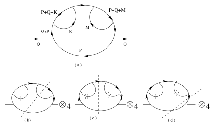
Figure 27: A three loop self energy and its cuts.

The thermal factors for Figs.[27b-d] are respectively,

$$\frac{1}{2}N(k){\cal N}(p+q+m;m,p)$$

$$\frac{1}{4}N(k)N(m){\cal N}(p+q;p)$$

$$\frac{1}{4}N(m)N(k){\cal N}(p+q;p)$$

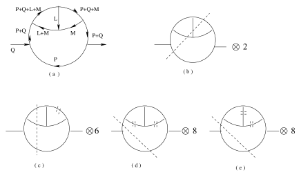
Figure 28: A three loop self energy and its cuts.

The thermal factors for Figs.[28b-e] are respectively,

$${\cal N}(p+q+m,l;p,l+m)$$

$$\frac{1}{2}N(p+q+m){\cal N}(p+q+l+m;p,l+m)$$

$$\frac{1}{4}N(m)N(l+m){\cal N}(p+q;p)$$

$$\frac{1}{4}N(l)N(m){\cal N}(p+q;p)$$

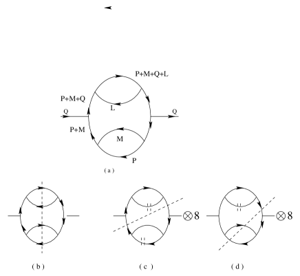
Figure 29: A three loop self energy and its cuts.

The thermal factors for Figs.[29b-d] are respectively,

$${\cal N}(p+q+m+l;p,m,l)$$

$$\frac{1}{4}N(l)N(p){\cal N}(p+q+m;p+m)$$

$$\frac{1}{2}N(l){\cal N}(p+q+m;p,m)$$

Figure 30: A three loop self energy and its cuts.

The thermal factors for Figs.[30b-g] are respectively,

$${\cal N}(p+q,m,k;p+m+k)$$

$$\frac{1}{2}N(k){\cal N}(p+q,m;p+m)$$

$$\frac{1}{4}N(k)N(m){\cal N}(p+q;p)$$

$$\frac{1}{4}N(m)N(p+m+k){\cal N}(p+q;p)$$

$$\frac{1}{4}N(k)N(p+m){\cal N}(p+q;p)$$

$$2[(1+n_{k})n_{p+m+k}+n_{k}(1+n_{p+m+k})]{\cal N}(p+q;p)$$

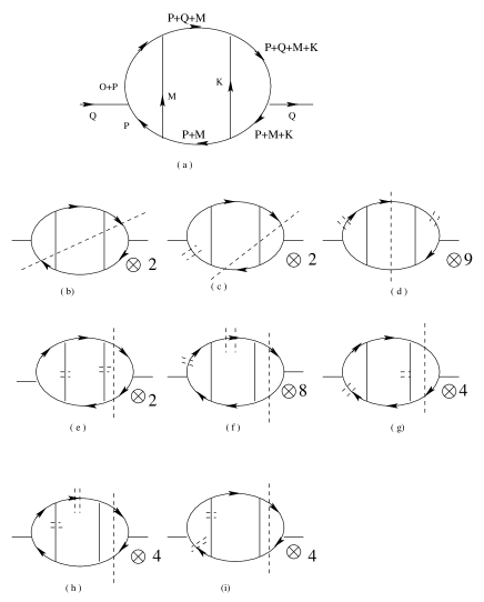
Figure 31: A three loop self energy and its cuts.

The thermal factors for Figs.[31b-i] are respectively,

$${\cal N}(p+q+m+k;k,m,p)$$

$$\frac{1}{2}N(p){\cal N}(p+q+m+k;k,p+m)$$

$$\frac{1}{4}N(q+p)N(q+p+m+k){\cal N}(p+q+m;p+m)$$

$$\frac{1}{4}N(m)N(k){\cal N}(p+q+m+k;p+m+k)$$

$$\frac{1}{4}N(p+q)N(p+q+m){\cal N}(p+q+m+k;p+m+k)$$

$$\frac{1}{4}N(p)N(k){\cal N}(p+q+m+k;p+m+k)$$

$$\frac{1}{4}N(m)N(p+q+m){\cal N}(p+q+m+k;p+m+k)$$

$$2[(1+n_{m})(1+n_{p})+n_{m}n_{p}]{\cal N}(p+q+m+k;p+m+k)$$

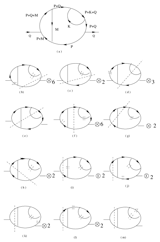
Figure 32: A four loop self energy and its cuts.

The thermal factors for Figs.[32b-m] are respectively,

$$\frac{1}{4}N(k)N(p+m){\cal N}(p+q;p)$$

$$\frac{1}{2}N(k){\cal N}(p+q,m;p+m)$$

$$\frac{1}{2}N(p+m+q){\cal N}(p+q+k;p,k)$$

$${\cal N}(p+q+k,m;p+m,k)$$

$$\frac{1}{4}N(k)N(m){\cal N}(p+q;p)$$

$$\frac{1}{2}N(k){\cal N}(p+q,m;p+m)$$

$$\frac{1}{2}N(k){\cal N}(p+q+m;p,m)$$

$$\frac{1}{4}N(k)N(m){\cal N}(p+q+m;p+m)$$

$$\frac{1}{4}N(k)N(p){\cal N}(p+q+m;p+m)$$

$$\frac{1}{4}N(k)N(p+q){\cal N}(p+q+m;p+m)$$

$$\frac{1}{4}N(k)N(p+q){\cal N}(p+q+m;p+m)$$

$$2[(1+n_{k})n_{q+p+k}+n_{k}(1+n_{q+p+k})]{\cal N}(p+q+m;p+m)$$

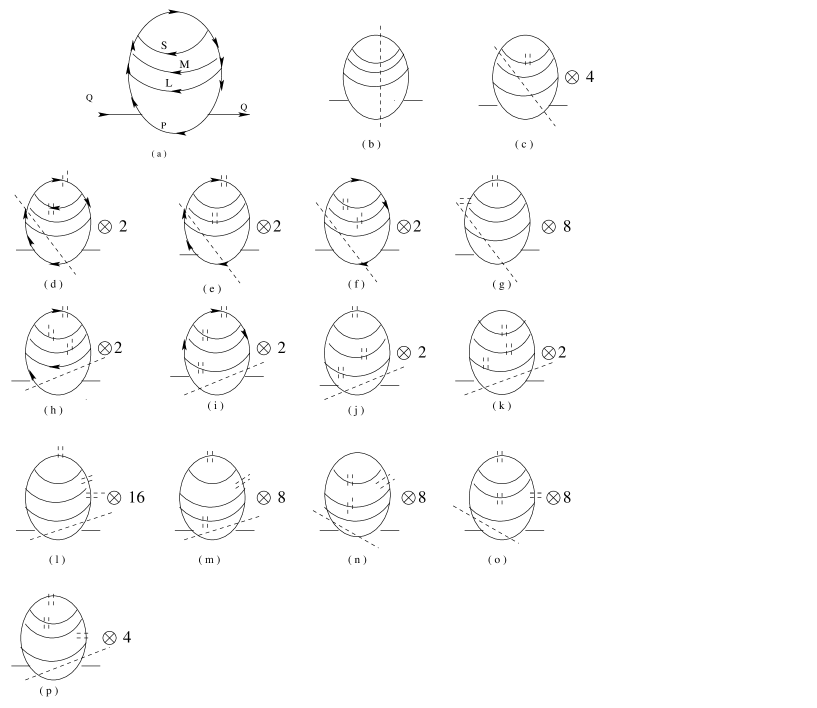
Figure 33: A four loop self energy and its cuts.

The thermal factors for Figs.[33b-p] are respectively,

$${\cal N}(p+q+m+l+s;s,m,l,p)$$

$$\frac{1}{2}N(s){\cal N}(p+q+m+l;m,l,p)$$

$$2[(1+n_{s})n_{p+q+m+l+s}+n_{s}(1+n_{p+q+m+l+s})]{\cal N}(p+q+l;l,p)$$

$$\frac{1}{4}N(p+q+m+l+s)N(m){\cal N}(p+q+l;l,p)$$

$$\frac{1}{4}N(s)N(m){\cal N}(p+q+l;l,p)$$

$$\frac{1}{4}N(p+q+m+l+s)N(p+q+l+m){\cal N}(p+q+l;l,p)$$

$$2[(1+n_{p+q+m+l+s}n_{s}n_{m}+n_{p+q+m+l+s}(1+n_{s})(1+n_{m})]{\cal N}(p+q;p)$$

$$N(l)[(1+n_{p+q+m+l+s})n_{s}+n_{p+q+m+l+s}(1+n_{s})]{\cal N}(p+q;p)$$

$$\frac{1}{8}N(p+q+m+l+s)N(m)N(l){\cal N}(p+q;p)$$

$$\frac{1}{8}N(s)N(m)N(l){\cal N}(p+q;p)$$

$$\frac{1}{8}N(p+q+m+l+s)N(p+q+m+l)N(p+q+l){\cal N}(p+q;p)$$

$$\frac{1}{8}N(p+q+m+l+s)N(p+q+m+l)N(l){\cal N}(p+q;p)$$

$$N(s)[(1+n_{p+q+m+l}n_{m}+n_{p+q+m+l}(1+n_{m})]{\cal N}(p+q;p)$$

$$\frac{1}{8}N(m)N(p+q+m+l+s)N(p+q+l){\cal N}(p+q;p)$$

$$N(p+q+l)[(1+n_{p+q+m+l+s})n_{s}+n_{p+q+m+l+s}(1+n_{s})]{\cal N}(p+q;p)$$

VI Conclusions

In this paper we have discussed a set of rules for calculating the imaginary parts of self energy diagrams as a series of tree amplitudes which represent physical scattering processes. The thermal factors associated with each scattering diagram have a physical interpretation in terms of the statistical weighting factors associated with the emission and absorption of thermal fields. Work on a general derivation of these rules from first principles is in progress.

References

- (1) H.A. Weldon, Phys. Rev. D28 (1983) 2007.
- (2) S.M.H. Wong, Phys. Rev. D64 (2001) 025007.
- (3) A. Majumder and C. Gale, hep-ph/0111181.
- (4) R.L. Kobes and G.W. Semenoff, Nucl. Phys. B 260 (1985) 714; R.L. Kobes and G.W. Semenoff, Nucl. Phys. B 272 (1986) 329.
- (5) F. Gelis, Nuc. Phys. B 508 483 (1997).
- (6) P. Aurenche, F. Gelis, R. Kobes and H. Zaraket, Phys. Rev. D60 076002 (1999).
- (7) F.T. Brandt, Ashok Das, J. Frenkel and A.J. daSilva, Phys. rev. D59 065004 (1999); F.T. Brandt, Ashok Das and J. Frenkel, Phys. Rev. D60 105008 (1999).
- (8) M.E. Carrington, Hou Defu, A. Hachkowski, D. Pickering and J.C. Sowiak, Phys. Rev. D61 25011 (2000).