Role of quantum fluctuations at high energies

Abstract

In this report we investigate an influence of virtual particles on the classical motion of a system in Minkowski and Euclidean spaces. Our results indicate that fluctuations of fields different from the main field decelerate significantly its motion at high energies. The formalism described here is applicable to the majority of inflationary models. A smallness of temperature fluctuation of cosmic relic background could be explained within this framework.

We show also that the quantum fluctuations suppress false vacuum decay in first-order phase transitions at high energies.

1. Massive fields and inflation

The first models of inflation solved many conceptual problems. The price was, in general, very small coupling constants. For example, one of the most promising model, chaotic inflation [1], with the potential of the form $\lambda\varphi^{4}$ gives $\lambda\sim 10^{-13}$ to be compatible with large-scale temperature fluctuations. To overcome this difficulty, it seems necessary to take a second field into consideration with a specific coupling to the first one, as was done in many modern inflationary scenarios. For example, hybrid inflation [2] deals with two coupled scalar fields with connected classical equations of motion. There are models which take into consideration an interaction of a classical field with particles, which are produced by the main field during a classical motion [3, 4, 5].

Here we consider only a pure quantum effect of interaction of the main field with virtual particles of some other sort. Temperature effects are not considered here. It is known that a cloud of virtual particles, having inertia, is able to decelerate the motion of the classical field, which produces this virtual cloud. This phenomena is well known in solid state physics (polaron effect, see e.g.[6, 7]).

To show and discuss the main effect, consider only one auxiliary scalar field $\chi$ as a representative of all other fields coupled to an inflaton field $\varphi$. The form of interaction is chosen in such a way to obtain analytical results:

$$S=\int d^{4}x\sqrt{-g}\left[\frac{1}{2}\varphi_{,\mu}\varphi^{,\mu}-V(\varphi)+\frac{1}{2}\chi_{,\mu}\chi^{,\mu}-\frac{1}{2}m_{\chi}^{2}\chi^{2}-\kappa\chi u(\varphi)\right].$$ (1)

Here $u(\varphi)$ is the polynomial of $\varphi$ with a power less than 3 for renormalazable theories. The first power of field $\chi$ permits one to obtain final formulae which are valid for some arbitrary coupling constant $\kappa$. $\chi$ - particles are supposed to be virtual, and thus the transition amplitude has the form

$$A(\varphi_{i},\chi_{i}=0\chi;\varphi_{f},\chi_{f}=0)=\int_{\varphi_{i}}^{\varphi_{f}}D\varphi\int_{0}^{0}D\chi\exp\left[iS\right].$$ (2)

Here the field $\chi$ is considered to be rather massive, so that its classical component is placed at a minimum of its potential. Integrating out the field variable $\chi$ one arrives at the effective action

$$S_{eff}=\int d^{4}x\sqrt{-g}\left[\frac{1}{2}\varphi_{,\mu}\varphi^{,\mu}-V(\varphi)\right]+\frac{\kappa^{2}}{2}\int d^{4}x\int d^{4}x^{\prime}\sqrt{-g}u(\varphi(x))G(x,x^{\prime})u(\varphi(x^{\prime}))$$ (3)

This expression is exact, but the nonlocal term prohibits to make analytical predictions. To proceed, let us expand the nonlocal term (3) into a power series of $x-x^{\prime}$ just like in the method of effective action [8]. The simplest way is to use the equation for the Green function [9] in the form

$$G(x,x^{\prime})=\frac{1}{m_{\chi}^{2}\sqrt{-g}}\delta(x-x^{\prime})-\frac{1}{m_{\chi}^{2}}\frac{1}{\sqrt{-g}}\partial_{\mu}\sqrt{-g}\partial^{\mu}G(x,x^{\prime})$$ (4)

Substituting it into expression (3) and neglecting higher derivatives of field $\varphi$ (recall that we are going to deal with slow motion), one obtains

$$S_{eff}=\int d^{4}x\sqrt{-g}\left[\frac{1}{2}\varphi_{,\mu}\varphi^{,\mu}-V_{ren}(\varphi)-\frac{1}{\sqrt{-g}}\frac{\kappa^{2}}{2m_{\chi}^{4}}u(\varphi)\partial_{\mu}\sqrt{-g}\partial^{\mu}u(\varphi)\right]$$ (5)

The first term in Eq.(4) contributes to renormalization of initial parameters of the potential. The last term in Eq.(5) changes the form of kinetic term. As parameters of potential will be determined by some physical conditions, we will concentrate on new terms in the kinetic energy which cannot be incorporated into parameter renormalization. The importance of this is discussed in [10] in connection with the cosmological constant problem.

The classical equation of motion can be written

$$\partial_{\mu}\sqrt{-g}\partial^{\mu}\varphi+\sqrt{-g}V_{ren}^{\prime}(\varphi)+{\frac{\alpha^{2}}{m_{\chi}^{2}}}u_{\varphi}^{\prime}(\varphi)\partial_{\mu}\sqrt{-g}\partial^{\mu}u(\varphi)=0,$$ (6)

where $\alpha\equiv\frac{\kappa}{m_{\chi}}$.

Renormalized parameters contain contributions from interactions with all fields and the field $\chi$ being among them. The latter contributes to renormalization of the coupling constant $\lambda_{ren}$ and can be written explicitly - $\delta\lambda_{ren}^{(\chi)}=-\frac{\alpha^{2}}{2}$. The main shortcoming of the first model of chaotic inflation with the potential of the form $\lambda_{ren}\varphi^{4}$ was a smallness of the coupling constant $\lambda_{ren}(\sim 10^{-13})$ necessary to avoid contradiction with observations. It means that all terms in the final expression for $\lambda_{ren}$ including $\delta\lambda_{ren}^{(\chi)}$ must be cancelled with a high accuracy. Below it is shown that renormalization of the kinetic term permits one to weaken restrictions for parameters of the theory.

The inflaton field is considered homogeneous during the period of inflation, $\varphi=\varphi(t)$ and Eq.(6) becomes more simple. One can neglect terms proportional to $d^{2}\varphi/dt^{2}$ and $(d\varphi/dt)^{2}$ taking into account slow motion of the field $\varphi$, which takes place under condition

$$\varphi\gg\varphi_{c}\equiv\frac{m_{\chi}}{{2\alpha}},$$ (7)

It leads to a classical equation of the form

$${\frac{12H\alpha^{2}}{m_{\chi}^{2}}}\varphi^{2}\dot{\varphi}+V_{ren}^{\prime}(\varphi)=0.$$ (8)

On deriving this equation, the usual connection of the scale factor $a(t)$ and Hubble parameter $H$ - $H=\dot{a}/a$ was assumed to hold. Consider as a specific case $u(\varphi)=\varphi^{2}$ and $V(\varphi)=\lambda\varphi^{n}$. Then the solution of Eq.(8) can be written

$$\varphi(t)=\left[\varphi_{0}^{4-n/2}-t/f_{n}\right]^{1/(4-n/2)},f_{n}=\frac{8\sqrt{6\pi}}{n(4-n/2)}\frac{\kappa^{2}}{m_{\chi}^{4}M_{p}\lambda^{1/2}}.$$ (9)

Here the following expression for the Hubble parameter $H=\sqrt{8\pi V(\varphi)/3}/M_{P}$ was used. The condition of slow motion is ${\ddot{\varphi}}<<12H\varphi^{2}{\dot{\varphi}}{\frac{\alpha^{2}}{m_{\chi}^{2}}}$. It is important to mention that the velocity of motion

$$\dot{\varphi}={\frac{m^{2}}{12\alpha^{2}\varphi^{2}}}\cdot\frac{V^{\prime}}{H},$$

obtained from Eqs. (8) appears to be much smaller than the usual value [1],

$$\dot{\varphi}=\frac{V^{\prime}}{3H},$$

which justifies our initial assumption. First, a ’superslow’ stage of inflation is finished when $\varphi\sim\varphi_{c}$. Then the stage of ordinary inflation takes place until ${\ddot{\varphi}}<<3H{\dot{\varphi}}$.

Let us determine an amplitude of quantum fluctuations during the ’superslow’ stage of inflation. Fluctuations of noninteracting fields were investigated before [1]. At the same time only estimations of order of magnitude are known for interacting fields [11]. The probability of given fluctuations developed for a cosmological time $\sim 1/H$ in a causally connected region with the size $\sim 1/H$ is not small if the action is not large as compared with unity, $\Delta S\leq 1,\quad\hbar=1$. The main contribution gives the last term in Eq.(5):

$$1\sim\Delta S_{eff}\sim\frac{2\kappa^{2}}{m_{\chi}^{4}}\frac{1}{H^{3}}\varphi^{2}\frac{\Delta\varphi^{2}}{H^{-1}}$$

and hence

$$\Delta\varphi\sim\frac{m_{\chi}}{\alpha\varphi}H.$$ (10)

Thus, the amplitude of fluctuations are proven to be small as compared with those in the case of ordinary inflation $H/2\pi$ or as compared with the estimation $H/\lambda^{1/4}$ on the basis of the term $V(\varphi)=\lambda\varphi^{4}$, [11]. It should be mentioned that in terms of the quasifield $\widetilde{\varphi}=\varphi^{2}$ the high - energy behaviour looks just like that for a free massive field.

To proceed let us find the field value $\varphi_{U}$ when our Universe was born. It is known that $N_{U}\simeq 60$ e-folgings enough to explain the main observational data. Taking into account the connection $N_{U}=\int_{\varphi_{U}}^{\varphi_{final}}Hdt$, we obtain

$$\varphi_{U}\simeq\left(\frac{N_{U}}{2\pi}\right)^{1/4}\sqrt{\frac{M_{P}m_{\chi}}{\alpha}}.$$ (11)

One can see that our Universe could be nucleated rather late due to the effect of virtual particles if $m_{\chi}<<M_{P}$. It does not seem strange because the first stage of inflation is characterized by a ’superslow’ motion, and the Universe has enough time for an appropriate expansion.

All discussion above holds if quanta of the auxiliary field $\chi$ are quite heavy, and the field is at a minimum of its potential during the inflationary stage. It takes place if $H<m$. This inequality ought to hold at least during the first stage of inflation, when $\varphi_{U}\geq\varphi\geq\varphi_{c}$. Some simple calculations give the estimates

$$\begin{array}[]{l}m_{\chi}>H(\varphi_{U})\quad\to\quad\frac{{\sqrt{\lambda}}}{\alpha}\leq 0.1\\ m_{\chi}>H(\varphi_{c})\quad\to\quad m_{\chi}\leq M_{P}\frac{{\sqrt{\lambda}}}{{\alpha^{2}}}\\ \end{array}$$ (12)

which do not seem to be very strong. A lower limit for $m_{\chi}$ is determined at least by quantum corrections, and we have a plausible estimation $m_{\chi}\geq\kappa$ or, equivalently, $\alpha<1$.

Let us find a parameter range which does not contradict the observable temperature fluctuations of cosmic background radiation. Standard calculations [12, 13] where the expression (10) is taken into account leads to the equality

$$\frac{\delta\rho}{\rho}=16\sqrt{6\pi}N_{U}\frac{m_{\chi}}{M_{P}}\frac{\sqrt{\lambda}}{\alpha},$$

for the potential $\lambda\varphi^{4}$. According to the observational data [14], $\delta\rho/\rho\approx 6\cdot 10^{-5}$ at the scale of modern horizon. Thus one obtains only connection of parameters in our model

$$\frac{{\sqrt{\lambda}}}{\alpha}\frac{m_{\chi}}{{M_{P}}}\sim 10^{-8},$$ (13)

instead of a strong restriction for the parameter $\lambda$.

As a result, we can conclude that the collective motion of the inflaton field and virtual particles are able to explain observable small temperature fluctuations in a natural way.

2. Suppression of first-order phase transitions by virtual particles

In the following we show that the virtual particles decreases significantly the probability of vacuum decay even at zero temperature. It could lead to an alternation of the order of phase transitions at the early stage of evolution of our Universe.

Let us start with the double well potential of the scalar field with nondegenerate vacua. Following the logic discussed in the beginning of this paper, consider an auxiliary field $\chi$ with action (1). Phase transitions are investigated usually in Euclidean space, which means a substitution $t\rightarrow i\tau$ in the formulae written above.

The calculations similar to those in the first part lead to an effective Euclidean action for the scalar field $\varphi$

$$\begin{array}[]{l}S_{E}=\int{d^{4}x}\left[\frac{1}{2}(\partial\varphi)^{2}+V_{ren}(\varphi)\right]+\frac{{\alpha^{2}}}{2m_{\chi}^{2}}\int{d^{4}x}\left[\frac{{\partial u(\varphi(x))}}{{\partial x_{\mu}}}\right]^{2}.\end{array}$$ (14)

(Here and below gravitational effects are omitted).The last term can be interpreted as influence of the virtual $\chi$ - particles.

Let the field $\varphi$ be placed initially at a metastable minimum of the potential $V_{ren}$. In this case the decay of the vacuum goes by nucleation and expanding of bubbles with a true vacuum $\varphi_{T}$ inside it. The outer space is filled with a metastable phase $\varphi_{F}$. This process is described by O(4) - invariant solution $\varphi_{B}(r)$ of the classical equation of motion in Euclidean space with the boundary conditions $\varphi_{B}(0)=\varphi_{T};\varphi_{B}(\infty)=\varphi_{F}$. The probability of the vacuum decay was obtained in [15]

$$\Gamma/V=\left({\frac{{S_{E}(\varphi_{B})}}{{2\pi}}}\right)^{2}\left|{\frac{{Det^{\prime}\hat{D}(\varphi_{B})}}{{Det\hat{D}(\varphi_{F})}}}\right|^{-1/2}e^{-S_{E}(\varphi_{B})},$$ (15)

where the kernel $K$ of operator $\hat{D}(\varphi)$ has the form $K(x,y)\equiv\frac{\delta^{2}S_{E}(\varphi)}{\delta\varphi(x)\delta\varphi(y)}$. The effective action in the exponent is the main factor. On the other hand, as shown below, the value of the effective action orders of magnitude increases under the influence of virtual particles. Let us choose the potential in the form

$$V_{ren}=\frac{\lambda}{8}\left(\varphi^{2}-a^{2}\right)^{2}+\frac{\varepsilon}{2a}\left(\varphi-a\right).$$ (16)

The instanton solution of the Euclidean equation of motion for the field $\varphi$ may be parameterized in the following way

$$\varphi(x)=\varphi_{B}(r)=A\tanh\left(\frac{M}{2}(r-R)\right)-B,$$ (17)

were $r^{2}\equiv\sum_{\alpha=1}^{4}x_{\alpha}^{2}$. Parameters $R$ $M$ are to be determined by minimization of the action (8) while parameters $A$ $B$ are chosen to satisfy the boundary conditions

$$\begin{array}[]{l}\varphi_{B}(r\to\infty)=\varphi_{F};\\ \varphi_{B}(r\to 0)=\varphi_{T}.\end{array}$$ (18)

Higher derivatives are neglected in the expression (14) of the action. This approximation is correct if $\partial_{x}\varphi_{B}/m_{\chi}\varphi_{B}<<1$ ($m_{\chi}$ is the mass of $\chi$ - particles which are formed in a virtual cloud). On the other hand, the derivative of the instanton trajectory $\partial_{x}\varphi_{B}$ is of the order of the mass of the main particle $m_{\varphi}$. Numerical calculations indicate that the transition from a false vacuum to a true one becomes noticeably wider due to the influence of virtual particles, i.e. $M<<m_{\varphi}$. Thus our approximation is valid at least if $m_{\varphi}/m_{\chi}<<1$. A numerical O(4) - symmetrical solution of the equation

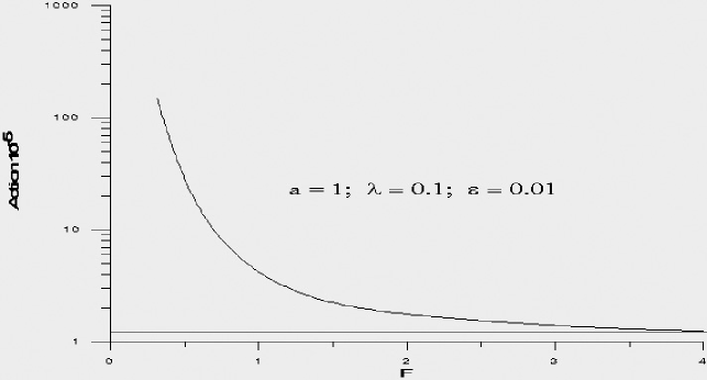
Figure 1: Dependence of the effective action on the parameter $F=2m_{\chi}^{2}/\alpha^{2}$

.

$$\begin{array}[]{l}\partial_{r}^{2}\varphi+\frac{3}{r}\partial_{r}\varphi-V^{\prime}(\varphi)+\\ +\frac{{\alpha^{2}}}{{m_{\chi}^{2}}}u^{\prime}(\varphi)\left[{\frac{3}{r}u^{\prime}(\varphi)\partial_{r}\varphi+u^{\prime\prime}(\varphi)(\partial_{r}\varphi)^{2}+u^{\prime}(\varphi)\partial_{r}^{2}\varphi}\right]=0\end{array}$$ (19)

is supposed to have the form (17). The results of calculations are represented in Fig.1. The horizontal line marks the standard result. The effect of virtual particles was not taken into account. Obviously, the effective action orders of magnitude increases, and the vacuum decay is exponentially suppressed comparable with the well-known result.

In conclusion, we found that virtual particles at high energies could significantly influence the classical motion and vacuum decay. It is shown that in a wide range of parameters the first stage of inflation consists of a ’superslow’ motion of the inflaton field. One of the useful effect of virtual particles is a considerable weakening of the conditions on parameters given by observational data. Tunnelling processes could be strongly forbidden as compared with a textbook result too.

Acknowledgement

SGR are grateful to A.S. Sakharov and M.Yu. Khlopov for their interest and useful discussion and A.A. Starobinsky for critical comments. The work of SGR was partially performed in the framework of Section ”Cosmoparticle physics” of Russian State Scientific Technological Programme ”Astronomy. Fundamental Space Research”, with support of Cosmion-ETHZ and Epcos-AMS collaborations.

References

- [1] A. D. Linde, The Large-scale Structure of the Universe (Harwood Academic Publishers, London, 1990).
- [2] A. D. Linde, Phys. Lett.B 259, 38 (1991).
- [3] A.D. Dolgov and S.H. Hansen, hep-ph/9810428 (1998).
- [4] A.N. Taylor and A. Berera, astro-ph/0006077 (2000).
- [5] I. Dymnikova and M.Yu. Khlopov, Mod.Phys.Lett. A15, 2305 (2000).
- [6] J. T. Devreese, Polarons in Ionic Crystals and Polar Semiconductors (North-Holland, Amsterdam, 1972).
- [7] A. B. Krebs and S. G. Rubin, Phys.Rev.B 49, 11808 (1994).
- [8] C. Itzykson and J.-B. Zuber, Quantum Field Theory, ed. (McGraw-Hill, New York, 1984).
- [9] N.D. Birrell and P.C.W. Davies, Quantum Fields in Qurved Space, Vol. of (Cambridge Univ. Press, Cambridge London New York Sydney, 1982).
- [10] J. Garriga and A. Vilenkin, hep-th/0011262, 2001.
- [11] A.D. Dolgov, Phys. Reports 222, 309 (1992).
- [12] J.M. Bardeen, P.J. Steinhardt, and M.S. Turner, Phys.Rev.D 28, 679 (1983).
- [13] V.F. Mukhanov, H.A. Feldman, and R.H. Brandenberger, Phys. Reports 215, 203 (1992).
- [14] C.L. Bennett et al., Astrophys.J.Lett. 464, 1 (1996).
- [15] S. Coleman, Phys. Rev. D 15, 2929 (1977).