xxx

LAL 02-39

TUM-HEP-465/02

October 2002

The CKM Matrix and The Unitarity Triangle:

Another Look

Andrzej J. Buras¹⁾, Fabrizio Parodi²⁾ and Achille Stocchi³⁾

¹⁾ Technische Universität München, Physik Department

D-85748 Garching, Germany

²⁾ Dipartimento di Fisica, Universita’ di Genova and INFN

Via Dodecaneso 33, 16146 Genova, Italy

³⁾ Laboratoire de l’Accélérateur Linéaire

IN2P3-CNRS et Université de Paris-Sud, BP 34, F-91898 Orsay Cedex

and CERN, 1211 Geneva 23, Switzerland

Abstract

The unitarity triangle can be determined by means of two measurements of its sides or angles. Assuming the same relative errors on the angles $(\alpha,\beta,\gamma)$ and the sides $(R_{b},R_{t})$, we find that the pairs $(\gamma,\beta)$ and $(\gamma,R_{b})$ are most efficient in determining $(\bar{\varrho},\bar{\eta})$ that describe the apex of the unitarity triangle. They are followed by $(\alpha,\beta)$, $(\alpha,R_{b})$, $(R_{t},\beta)$, $(R_{t},R_{b})$ and $(R_{b},\beta)$. As the set $|V_{us}|$, $|V_{cb}|$, $R_{t}$ and $\beta$ appears to be the best candidate for the fundamental set of flavour violating parameters in the coming years, we show various constraints on the CKM matrix in the $(R_{t},\beta)$ plane. Using the best available input we determine the universal unitarity triangle for models with minimal flavour violation (MFV) and compare it with the one in the Standard Model. We present allowed ranges for $\sin 2\beta$, $\sin 2\alpha$, $\gamma$, $R_{b}$, $R_{t}$ and $\Delta M_{s}$ within the Standard Model and MFV models. We also update the allowed range for the function $F_{tt}$ that parametrizes various MFV-models.

1 Introduction

The determination of the Cabibbo-Kobayashi-Maskawa (CKM) matrix [1, 2] that parametrizes the weak charged current interactions of quarks is one of the important targets of particle physics. During the last two decades several strategies have been proposed that should allow one to determine the CKM matrix and the related unitarity triangle (UT). They are reviewed in particular in [3, 4, 5, 6, 7].

To be specific let us first choose as the independent parameters

$$|V_{us}|,\qquad|V_{cb}|,\qquad\bar{\varrho},\qquad\bar{\eta}$$ (1.1)

where $(\bar{\varrho},\bar{\eta})$, defined below, determine the apex of the unitarity triangle in question. The best place to determine $|V_{us}|$ and $|V_{cb}|$ are the semi-leptonic K and B decays, respectively. The question that we want address here is the determination of the remaining two parameters $(\bar{\varrho},\bar{\eta})$.

There are many ways to determine $(\bar{\varrho},\bar{\eta})$. As the length of one side of the rescaled unitarity triangle is fixed to unity, we have to our disposal two sides, $R_{b}$ and $R_{t}$ and three angles, $\alpha$, $\beta$ and $\gamma$. These five quantities can be measured by means of rare K and B decays and in particular by studying CP-violating observables. While until recently only a handful of strategies could be realized, the present decade should allow several independent determinations of $(\bar{\varrho},\bar{\eta})$ that will test the KM picture of CP violation [2] and possibly indicate the physics beyond the Standard Model (SM).

The determination of $(\bar{\varrho},\bar{\eta})$ in a given strategy is subject to experimental and theoretical errors and it is important to identify those strategies that are experimentally feasible and in which hadronic uncertainties are as much as possible under control. Such strategies are reviewed in [3, 4, 5, 6, 7].

Here we want to address a different question. The determination of $(\bar{\varrho},\bar{\eta})$ requires at least two independent measurements. In most cases these are the measurements of two sides of the UT, of one side and one angle or the measurements of two angles. Sometimes $\bar{\eta}$ can be directly measured and combining it with the knowledge of one angle or one side of the UT, $\bar{\varrho}$ can be found. Analogous comments apply to measurements in which $\bar{\varrho}$ is directly measured. Finally in more complicated strategies one measures various linear combinations of angles, sides or $\bar{\varrho}$ and $\bar{\eta}$.

Restricting first our attention to measurements in which sides and angles of the UT can be measured independently of each other, we end up with ten different pairs of measurements that allow the determination of $(\bar{\varrho},\bar{\eta})$. The question then arises which of the pairs in question is most efficient in the determination of the UT? That is, given the same relative errors on $R_{b}$, $R_{t}$, $\alpha$, $\beta$ and $\gamma$, we want to find which of the pairs gives the most accurate determination of $(\bar{\varrho},\bar{\eta})$. This is one of the questions that we want to address here.

The answer to this question depends necessarily on the values of $R_{b}$, $R_{t}$, $\alpha$, $\beta$ and $\gamma$ but as we will see below just the requirement of the consistency of $R_{b}$ with the measured value of $|V_{ub}/V_{cb}|$ implies a hierarchy within the ten strategies mentioned above.

During the 1970’s and 1980’s the variables $\alpha_{QED}$, the Fermi constant $G_{F}$ and the sine of the Weinberg angle ($\sin\theta_{W}$) were the fundamental parameters in terms of which the electroweak tests of the SM have been performed. After the $Z^{0}$ boson has been discovered and its mass precisely measured at LEP-I, $\sin\theta_{W}$ has been replaced by $M_{Z}$ and the fundamental set used in the electroweak precision studies in the 1990’s has been $(\alpha_{QED},G_{F},M_{Z})$. It is to be expected that when $M_{W}$ will be measured precisely this set will be changed to $(\alpha_{QED},M_{W},M_{Z})$ or ($G_{F},M_{W},M_{Z})$.

We anticipate that an analogous development will happen in this decade in connection with the CKM matrix. While the set (1.1) has clearly many virtues and has been used extensively in the literature, one should emphasize that presently no direct independent measurements of $\bar{\eta}$ and $\bar{\varrho}$ are available. $|\bar{\eta}|$ can be measured cleanly in the decay $K_{L}\to\pi^{0}\nu\bar{\nu}$. On the other hand to our knowledge there does not exist any strategy for a clean independent measurement of $\bar{\varrho}$.

Taking into account the experimental feasibility of various measurements and their theoretical cleanness, the most obvious candidate for the fundamental set in the quark flavour physics for the coming years appears to be

$$|V_{us}|,\qquad|V_{cb}|,\qquad R_{t},\qquad\beta$$ (1.2)

with the last two variables describing the $V_{td}$ coupling that can be measured by means of the $B^{0}-\bar{B}^{0}$ mixing ratio $\Delta M_{d}/\Delta M_{s}$ and the CP-asymmetry $a_{\psi K_{S}}$, respectively. In this context we investigate, in analogy to the $(\bar{\varrho},\bar{\eta})$ plane and the planes $(\sin 2\beta,\sin 2\alpha)$ [8] and $(\gamma,\sin 2\beta)$ [9] considered in the past, the $(R_{t},\beta)$ plane for the exhibition of various constraints on the CKM matrix. We also provide the parametrization of the CKM matrix given directly in terms of the variables (1.2).

Several of the results and formulae presented here are not entirely new and have been already discussed by us and other authors in the past. In particular in [10] it has been pointed out that only a moderately precise measurement of $\sin 2\alpha$ can be as useful for the UT as a precise measurement of the angle $\beta$. This has been recently reemphasized in [11]. Similarly the measurement of the pair $(\alpha,\beta)$ has been found to be a very efficient tool for the determination of the UT [12, 13] and the construction of the full CKM matrix from the angles of various unitarity triangles has been presented in [14]. Finally the importance of the pair $(R_{t},\sin 2\beta)$ has been emphasized recently in a number of papers [15, 16, 17, 18, 19]. Many useful relations relevant for the unitarity triangle can also be found in [20, 21]. On the other hand, to our knowledge, no systematic classification of the strategies in question and their comparison has been presented in the literature and the discussion of the $(R_{t},\beta)$ plane is presented for the first time. We think that in view of the present and future efforts to determine the CKM matrix such a study is desirable.

Our paper is organized as follows. In section 2 we recall some formulae related to the CKM matrix and the UT. In section 3 we list the expressions for $\bar{\varrho}$ and $\bar{\eta}$ in the ten strategies in question and provide the parametrization of the CKM matrix directly in terms of the set (1.2). In section 4 we present a numerical analysis that reveals a hierarchy of various determinations and we show how various constraints appear in the different planes corresponding to the leading strategies. In section 5 we show the implications of the presently available strategies $(R_{t},\beta)$, $(R_{b},\beta)$ and $(R_{t},R_{b})$ in determining the allowed region for $(\bar{\varrho},\bar{\eta})$ and we present the available constraints on the CKM matrix in the $(R_{t},\beta)$ plane. In section 6 we determine the universal unitarity triangle for models with minimal flavour violation (MFV) and compare it with the one in the Standard Model. We also update the allowed range for the function $F_{tt}$ that parametrizes various MFV-models. We conclude in section 7.

2 CKM Matrix and the Unitarity Triangle

Many parametrizations of the CKM matrix have been proposed in the literature. The most popular are the standard parametrization [22] recommended by the Particle Data Group [23] and a generalization of the Wolfenstein parametrization [24] as presented in [12].

With $c_{ij}=\cos\theta_{ij}$ and $s_{ij}=\sin\theta_{ij}$ ($i,j=1,2,3$), the standard parametrization is given by:

$$\hat{V}_{\rm CKM}=\left(\begin{array}[]{ccc}c_{12}c_{13}&s_{12}c_{13}&s_{13}e^{-i\delta}\\ -s_{12}c_{23}-c_{12}s_{23}s_{13}e^{i\delta}&c_{12}c_{23}-s_{12}s_{23}s_{13}e^{i\delta}&s_{23}c_{13}\\ s_{12}s_{23}-c_{12}c_{23}s_{13}e^{i\delta}&-s_{23}c_{12}-s_{12}c_{23}s_{13}e^{i\delta}&c_{23}c_{13}\end{array}\right)\,,$$ (2.1)

where $\delta$ is the phase necessary for CP violation. $c_{ij}$ and $s_{ij}$ can all be chosen to be positive and $\delta$ may vary in the range $0\leq\delta\leq 2\pi$. However, the measurements of CP violation in $K$ decays force $\delta$ to be in the range $0<\delta<\pi$.

¿From phenomenological applications we know that $s_{13}$ and $s_{23}$ are small numbers: ${\cal O}(10^{-3})$ and ${\cal O}(10^{-2})$, respectively. Consequently, to an excellent accuracy, the four independent parameters are given as

$$s_{12}=|V_{us}|,\quad s_{13}=|V_{ub}|,\quad s_{23}=|V_{cb}|,\quad\delta.$$ (2.2)

The first three can be extracted from tree level decays mediated by the transitions $s\to u$, $b\to u$ and $b\to c$ respectively. The phase $\delta$ can be extracted from CP violating transitions or loop processes sensitive to $|V_{td}|$.

For our purposes it will be convenient to make the following change of variables in (2.1) [12, 25]

$$s_{12}=\lambda\,,\qquad s_{23}=A\lambda^{2}\,,\qquad s_{13}e^{-i\delta}=A\lambda^{3}(\varrho-i\eta)$$ (2.3)

where $\lambda$, $A$, $\varrho$ and $\eta$ are Wolfenstein parameters. It follows then that to a very good accuracy the set in (2.2) can be replaced by

$$|V_{us}|=\lambda,\qquad|V_{cb}|,\qquad\bar{\varrho},\qquad\bar{\eta}$$ (2.4)

where [12]

$$\bar{\varrho}=\varrho(1-\frac{\lambda^{2}}{2}),\qquad\bar{\eta}=\eta(1-\frac{\lambda^{2}}{2}).$$ (2.5)

The pair $(\bar{\varrho},\bar{\eta})$ describes the apex of the unitarity triangle shown in figure 1 that represents the unitarity relation

$$V_{ud}V_{ub}^{*}+V_{cd}V_{cb}^{*}+V_{td}V_{tb}^{*}=0$$ (2.6)

suitably rescaled by $|V_{cd}V_{cb}^{*}|=A\lambda^{3}=\lambda|V_{cb}|$, with the latter equalities satisfied to an excellent accuracy [7, 12].

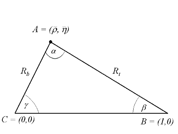
Figure 1: Unitarity Triangle.

Let us collect useful formulae related to this triangle:

• The lengths $CA$ and $BA$ to be denoted by $R_{b}$ and $R_{t}$, respectively, are given by

  $$R_{b}\equiv\frac{|V_{ud}V^{*}_{ub}|}{|V_{cd}V^{*}_{cb}|}=\sqrt{\bar{\varrho}^{2}+\bar{\eta}^{2}}=(1-\frac{\lambda^{2}}{2})\frac{1}{\lambda}\left|\frac{V_{ub}}{V_{cb}}\right|,$$ (2.7)

  $$R_{t}\equiv\frac{|V_{td}V^{*}_{tb}|}{|V_{cd}V^{*}_{cb}|}=\sqrt{(1-\bar{\varrho})^{2}+\bar{\eta}^{2}}=\frac{1}{\lambda}\left|\frac{V_{td}}{V_{cb}}\right|.$$ (2.8)

• The angles $\beta$ and $\gamma=\delta$ of the unitarity triangle are related directly to the complex phases of the CKM-elements $V_{td}$ and $V_{ub}$, respectively, through

  $$V_{td}=|V_{td}|e^{-i\beta},\qquad V_{ub}=|V_{ub}|e^{-i\gamma}.$$ (2.9)

• The unitarity relation (2.6) can be rewritten as

  $$R_{b}e^{i\gamma}+R_{t}e^{-i\beta}=1~{}.$$ (2.10)

• The angle $\alpha$ can be obtained through the relation

  $$\alpha+\beta+\gamma=180^{\circ}$$ (2.11)

  expressing the unitarity of the CKM-matrix.

The triangle depicted in figure 1, $|V_{us}|$ and $|V_{cb}|$ give the full description of the CKM matrix.

Formula (2.10) shows transparently that the knowledge of $(R_{t},\beta)$ allows to determine $(R_{b},\gamma)$ through [18]

$$R_{b}=\sqrt{1+R_{t}^{2}-2R_{t}\cos\beta},\qquad\cot\gamma=\frac{1-R_{t}\cos\beta}{R_{t}\sin\beta}.$$ (2.12)

Similarly, $(R_{t},\beta)$ can be expressed through $(R_{b},\gamma)$:

$$R_{t}=\sqrt{1+R_{b}^{2}-2R_{b}\cos\gamma},\qquad\cot\beta=\frac{1-R_{b}\cos\gamma}{R_{b}\sin\gamma}.$$ (2.13)

These formulae relate the leading strategy $(R_{t},\beta)$ for the determination of the so-called universal unitarity triangle [15] within the models with minimal flavour violation (MFV) [26] and the strategy $(R_{b},\gamma)$ that results in the so-called reference unitarity triangle as proposed and discussed in [27].

3 General Strategies

3.1 Basic Formulae

We list below the formulae for $\bar{\varrho}$ and $\bar{\eta}$ in the strategies that are labelled by the two measured quantities as discussed at the beginning of our paper.

3.1.1 $R_{t}$ and $\beta$

$$\bar{\varrho}=1-R_{t}\cos\beta,\qquad\bar{\eta}=R_{t}\sin\beta~{}.$$ (3.1)

3.1.2 $R_{b}$ and $\gamma$

$$\bar{\varrho}=R_{b}\cos\gamma,\qquad\bar{\eta}=R_{b}\sin\gamma~{}.$$ (3.2)

3.1.3 $R_{b}$ and $R_{t}$

$$\bar{\varrho}=\frac{1}{2}(1+R^{2}_{b}-R^{2}_{t}),\qquad\bar{\eta}=\sqrt{R_{b}^{2}-\bar{\varrho}^{2}}$$ (3.3)

where $\bar{\eta}>0$ has been assumed.

3.1.4 $R_{t}$ and $\gamma$

This strategy uses (3.2) with

$$R_{b}=\cos\gamma\pm\sqrt{R^{2}_{t}-\sin^{2}\gamma}~{}.$$ (3.4)

The two possibilities can be distinguished by the measured value of $R_{b}$.

3.1.5 $R_{b}$ and $\beta$

This strategy uses (3.1) and

$$R_{t}=\cos\beta\pm\sqrt{R^{2}_{b}-\sin^{2}\beta}~{}.$$ (3.5)

The two possibilities can be distinguished by the measured value of $R_{t}$.

3.1.6 $R_{t}$ and $\alpha$

$$\bar{\varrho}=1-R_{t}^{2}\sin^{2}\alpha+R_{t}\cos\alpha\sqrt{1-R_{t}^{2}\sin^{2}\alpha},$$ (3.6)

$$\bar{\eta}=R_{t}\sin\alpha\left[R_{t}\cos\alpha+\sqrt{1-R_{t}^{2}\sin^{2}\alpha}\right]$$ (3.7)

where $\cos\gamma>0$ has been assumed. For $\cos\gamma<0$ the signs in front of the square roots should be reversed.

3.1.7 $R_{b}$ and $\alpha$

$$\bar{\varrho}=R_{b}^{2}\sin^{2}\alpha-R_{b}\cos\alpha\sqrt{1-R_{b}^{2}\sin^{2}\alpha},$$ (3.8)

$$\bar{\eta}=R_{b}\sin\alpha\left[R_{b}\cos\alpha+\sqrt{1-R_{b}^{2}\sin^{2}\alpha}\right]$$ (3.9)

where $\cos\beta>0$ has been assumed.

3.1.8 $\beta$ and $\gamma$

$$R_{t}=\frac{\sin\gamma}{\sin(\beta+\gamma)},\qquad R_{b}=\frac{\sin\beta}{\sin(\beta+\gamma)}$$ (3.10)

and (3.3).

3.1.9 $\alpha$ and $\gamma$

$$R_{t}=\frac{\sin\gamma}{\sin\alpha},\qquad R_{b}=\frac{\sin(\alpha+\gamma)}{\sin\alpha}$$ (3.11)

and (3.3).

3.1.10 $\alpha$ and $\beta$

$$R_{t}=\frac{\sin(\alpha+\beta)}{\sin\alpha},\qquad R_{b}=\frac{\sin\beta}{\sin\alpha}$$ (3.12)

and (3.3).

Finally we give the formulae for the strategies in which $\bar{\eta}$ is directly measured and the strategy allows to determine $\bar{\varrho}$.

3.1.11 $\bar{\eta}$ and $R_{t}$ or $R_{b}$

$$\bar{\varrho}=1-\sqrt{R_{t}^{2}-\bar{\eta}^{2}},\qquad\bar{\varrho}=\pm\sqrt{R_{b}^{2}-\bar{\eta}^{2}}$$ (3.13)

where in the first case we have excluded the + solution in view of $R_{b}\leq 0.5$ as extracted from the experimental data on $|V_{ub}/V_{cb}|$.

3.1.12 $\bar{\eta}$ and $\beta$ or $\gamma$

$$\bar{\varrho}=1-\frac{\bar{\eta}}{\tan\beta},\qquad\bar{\varrho}=\frac{\bar{\eta}}{\tan\gamma}~{}.$$ (3.14)

3.2 CKM Matrix and the Fundametal Variables

It is useful for phenomenological purposes to express the CKM matrix directly in terms of the parameters selected in a given strategy. This can be easily done by inserting the formulae for $\bar{\varrho}$ and $\bar{\eta}$ presented here into the known expressions for the CKM elements in terms of these variables [24, 12] as given in section 2.

Here we give explicit result only for the set (1.2). In order to simplify the notation we use $\lambda$ instead of $|V_{us}|$ as $V_{us}=\lambda+{\cal O}(\lambda^{7})$. We find

$$V_{ud}=1-\frac{1}{2}\lambda^{2}-\frac{1}{8}\lambda^{4}+{\cal O}(\lambda^{6}),\qquad V_{ub}=\frac{\lambda}{1-\lambda^{2}/2}|V_{cb}|\left[1-R_{t}e^{i\beta}\right],$$ (3.15)

$$V_{cd}=-\lambda+\frac{1}{2}\lambda|V_{cb}|^{2}-\lambda|V_{cb}|^{2}\left[1-R_{t}e^{-i\beta}\right]+{\cal O}(\lambda^{7}),$$ (3.16)

$$V_{cs}=1-\frac{1}{2}\lambda^{2}-\frac{1}{8}\lambda^{4}-\frac{1}{2}|V_{cb}|^{2}+{\cal O}(\lambda^{6}),$$ (3.17)

$$V_{tb}=1-\frac{1}{2}|V_{cb}|^{2}+{\cal O}(\lambda^{6}),\qquad V_{td}=\lambda|V_{cb}|R_{t}e^{-i\beta}+{\cal O}(\lambda^{7}),$$ (3.18)

$$V_{ts}=-|V_{cb}|+\frac{1}{2}\lambda^{2}|V_{cb}|-\lambda^{2}|V_{cb}|\left[1-R_{t}e^{-i\beta}\right]+{\cal O}(\lambda^{6})~{}.$$ (3.19)

4 Hierarchies

The numerical analysis of various strategies listed in the previous section was performed using a Bayesian approach as described in [28].
Considering two measured quantities $x$ and $y$ the bidimensional probability density function for $x$ and $y$ is given (after appropriate normalization) by:

$$f(x,y)\propto{\cal L}(x){\cal L}(y)f_{o}(x,y)$$

where $f_{o}$ is the prior probability density function for $x$, $y$ (taken uniform all over the range) and ${\cal L}(x)$, ${\cal L}(y)$ represent the likelihood functions of the two measurements (assumed as a Gaussian distribution).
The probability density function for $\bar{\eta}$ and $\bar{\rho}$ ($f(\bar{\rho},\bar{\eta})$) is then obtained from $f(x,y)$ by changing the variables using the equations of the previous chapter. The probability density functions for $\bar{\rho}$ ($\bar{\eta}$) is then obtained by integrating $f$ over $\bar{\eta}$ ($\bar{\rho}$).

The main results of this analysis are depicted in figures 2, 3, 4 and 5. In figures 2 and 3 we plot the correlation between the precisions on the variables relevant for a given strategy required to reach the assumed precision on $\bar{\eta}$ and $\bar{\varrho}$, respectively. For this exercise we have used, for $\bar{\eta}$ and $\bar{\rho}$, the central values obtained using the input of table 1.

Obviously strategies described by curves in figures 2 and 3 that lie far from the origin are more effective in the determination of the unitarity triangle than those corresponding to curves placed close to the origin.

Figures 2 and 3 reveal certain hierarchies within the strategies in question. In order to find these hierarchies and to eliminate the weakest ones not shown in these figures we divided first the five variables under consideration into two groups:

$$(R_{t},\alpha,\gamma),\qquad(R_{b},\beta)~{}.$$ (4.1)

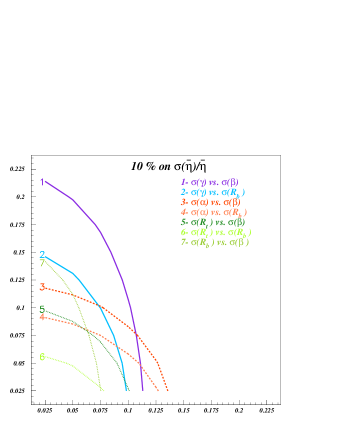
Figure 2: The plot shows the curves of the 10$\%$ relative precision on $\bar{\eta}$ as a function of the precision on the variables of the given strategy.

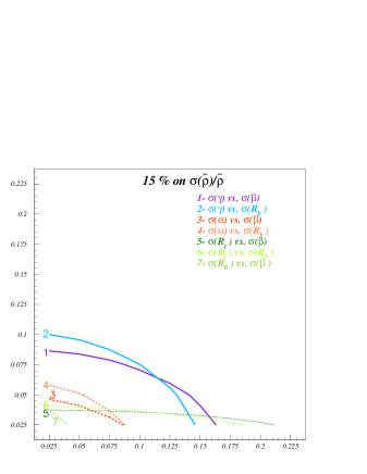
Figure 3: The plot shows the curves of the 15$\%$ relative precision on $\bar{\varrho}$ as a function of the precision on the variables of the given strategy.

It turned out then that the four strategies $(R_{t},\alpha)$, $(R_{t},\gamma)$, $(\alpha,\gamma)$ and $(R_{b},\beta)$ which involve pairs of variables belonging to the same group are not particularly useful in the determination of $(\bar{\varrho},\bar{\eta})$. In the case of $(R_{b},\beta)$ this is related to the existence of two possible solutions as stated above. If one of these solutions can easily be excluded on the basis of $R_{t}$, then the effectiveness of this strategy can be increased. We have therefore included this strategy in our numerical analysis. The strategy $(R_{t},\gamma)$ turns out to be less useful in this respect. Similarly the strategy $(\gamma,\alpha)$ is not particularly useful due to strong correlation between the variables in question as discussed previously by many authors in the literature.

The remaining six strategies that involve pairs of variables belonging to different groups in (4.1) are all interesting. While some strategies are better suited for the determination of $\bar{\eta}$ and the other for $\bar{\varrho}$, as clearly seen in figures 2 and 3, on the whole a clear ranking of strategies seems to emerge from our analysis.

If we assume the same relative error on $\alpha$, $\beta$, $\gamma$, $R_{b}$ and $R_{t}$ we find the following hierarchy:

$$1)~{}(\gamma,\beta),\quad(\gamma,R_{b})\qquad 2)~{}(\alpha,\beta),\quad(\alpha,R_{b})\qquad 3)~{}(R_{t},\beta),\quad(R_{t},R_{b}),\quad(R_{b},\beta).$$ (4.2)

We observe that in particular the strategies involving $R_{b}$ and $\gamma$ are very high on this ranking list. This is related to the fact that $R_{b}<0.5<R_{t}$ and consequently the action in the $(\bar{\varrho},\bar{\eta})$ plane takes place closer to the origin of this plane than to the corner of the UT involving the angle $\beta$. Consequently the accuracy on $R_{b}$ and $\gamma$ does not have to be as high as for $R_{t}$ and $\beta$ in order to obtain the same accuracy for $(\bar{\varrho},\bar{\eta})$. This is clearly seen in figures 2 and 3.

This analysis shows how important is the determination of $R_{b}$ and $\gamma$ in addition to $\beta$ that is already well known. On the other hand the strategy involving $R_{t}$ and $\beta$ will be most probably the cleanest one before the LHC experiments unless the error on $\gamma$ from B-factories and Tevatron can be decreased to $10^{\circ}$ and $R_{b}$ is significantly better known.

The strategies involving $\alpha$ are in our second best class. However, it has to be noticed that in order to get 10$\%$(15$\%$) relative precision on $\bar{\eta}$($\bar{\rho}$) it is necessary (see figures 2 and 3) to determine $\alpha$ with better than 10$\%$ relative precision. If $\sin 2\alpha$ could be directly measured this could be soon achieved due to its high sensitivity to $\alpha$ [10, 11]. However, from the present perspective a direct measurement of $\sin 2\alpha$ appears to be very difficult in view of the penguin pollution that could be substantial in view of the most recent data from Belle [29]. On the other hand, as the BaBar data [30] do not signal this pollution, it may eventually turn out that a useful direct measurement of $\sin 2\alpha$ can be soon achieved. The most recent theoretical discussions can be found in [31].

We have also performed a numerical analysis for the strategies in which $|\bar{\eta}|$ can be directly measured. The relevant formulae are given in (3.13) and (3.14). It turns out that the strategy $(\gamma,\bar{\eta})$ can be put in the first best class in (4.2) together with the strategies $(\gamma,\beta)$ and $(\gamma,R_{b})$.

In figure 4 we show the resulting regions in the $(\bar{\varrho},\bar{\eta})$ plane obtained from leading strategies assuming that each variable is measured with $10\%$ accuracy. This figure is complementary to figures 2 and 3 and demonstrates clearly the ranking given in (4.2).

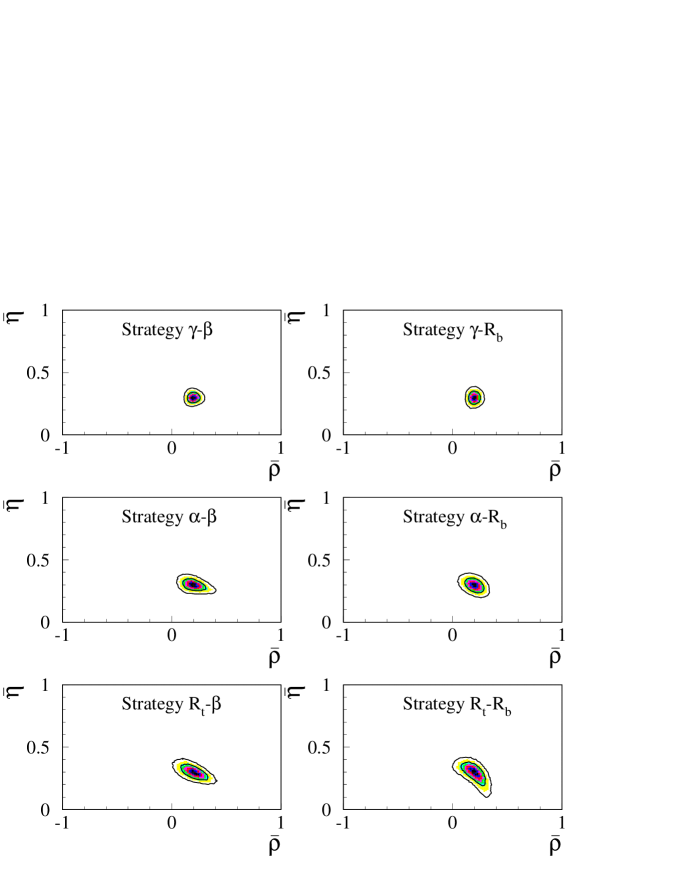
Figure 4: The plots show the allowed probability regions (68$\%$ and 95$\%$) in the $(\bar{\varrho},\bar{\eta})$ plane obtained from the leading strategies assuming that each variable is measured with $10\%$ accuracy.

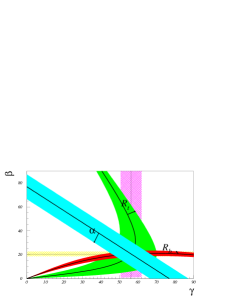
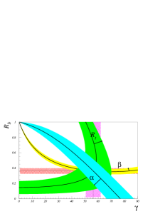
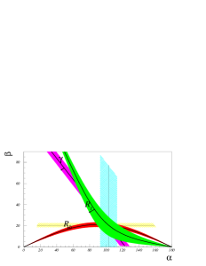
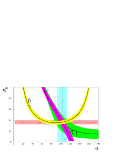
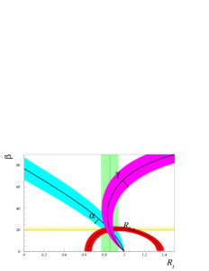
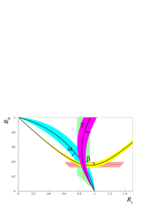
Figure 5: The plots show the different constraints (assuming a relative error of 10$\%$) in the different planes corresponding to the leading stategies of equation 4.2. The small arrow indicates the range corresponding to an increase of 10$\%$ of the corresponding quantity.

While at present the set (1.2) appears to be the leading candidate for the fundamental parameter set in the quark flavour physics for the coming years, it is not clear which set will be most convenient in the second half of this decade when the B-factories and Tevatron will improve considerably their measurements and LHC will start its operation. Therefore it is of interest to investigate how the measurements of three variables out of $\alpha,~{}\beta,~{}\gamma~{},R_{b}$ and $R_{t}$ will determine the allowed values for the remaining two variables. We illustrate this in figure 5 assuming a relative error of $10\%$ for the constraints used in each plot. While this figure is self explanatory a striking feature consistent with the hierarchial structure in (4.2) can be observed. While the measurements of $(\alpha,R_{t},R_{b})$ and $(\alpha,\beta,R_{t})$ as seen in the first two plots do not appreciably constrain the parameters of the two leading strategies $(\beta,\gamma)$ and $(R_{b},\gamma)$, respectively, the opposite is true in the last two plots. There the measurements of $(R_{b},\gamma,\alpha)$ and $(\beta,\gamma,\alpha)$ give strong constraints in the $(\beta,R_{t})$ and $(R_{b},R_{t})$ plain, respectively.

The last two plots illustrate also clearly that measuring only $\alpha$ and $\gamma$ does not provide a strong constraint on the unitarity triangle.

Finally we would like to emphasize that our ranking does not take into account the fact that the assumed precision on some variables can be easier to achieve than for other variables. While this is difficult to incorporate into our analysis at present, it could be in principle possible when our understanding of theoretical uncertainties in various determinations improves.

5 Presently available strategies

Parameter	Value	Gaussian	Uniform	Ref.
		$\sigma$	half-width
$\lambda$	$0.2210$	0.0020	-	[34]
$\left|V_{cb}\right|$(excl.)	$42.1\times 10^{-3}$	$2.1\times 10^{-3}$	-	[35]
$\left|V_{cb}\right|$(incl.)	$40.4\times 10^{-3}$	$0.7\times 10^{-3}$	$0.8\times 10^{-3}$	[35]
$\left|V_{cb}\right|$(ave.)	$40.6\times 10^{-3}$	$0.8\times 10^{-3}$ ∗
$\left|V_{ub}\right|$(excl.)	$32.5\times 10^{-4}$	$2.9\times 10^{-4}$	$5.5\times 10^{-4}$	[34]
$\left|V_{ub}\right|$(incl.)	$40.9\times 10^{-4}$	$4.6\times 10^{-4}$	$3.6\times 10^{-4}$	[34]
$\left|V_{ub}\right|$(ave.)	$36.3\times 10^{-4}$	$3.2\times 10^{-4}$ ∗
$\left|V_{ub}\right|$/$\left|V_{cb}\right|$(ave.)	0.089	0.008∗
$\Delta M_{d}$	$0.503~{}\mbox{ps}^{-1}$	$0.006~{}\mbox{ps}^{-1}$	–	[36]
$\Delta M_{s}$	$>$ 14.4 ps-1 at 95% C.L.	sensitivity 19.2 ps-1		[36]
$m_{t}$	$167~{}GeV$	$5~{}GeV$	–	[38]
$f_{B_{d}}\sqrt{\hat{B}_{B_{d}}}$	$235~{}MeV$	$33~{}MeV$	${}^{+0}_{-24}~{}MeV$	[37]
$\xi=\frac{f_{B_{s}}\sqrt{\hat{B}_{B_{s}}}}{f_{B_{d}}\sqrt{\hat{B}_{B_{d}}}}$	1.18	0.04	${}^{+0.12}_{-0.00}$	[37]
$\hat{B}_{K}$	0.86	0.06	0.14	[37]
sin 2$\beta$	0.734	0.054	-	[33]

Table 1: Values of the relevant quantities entering into the expressions of $|V_{ub}/V_{cb}|$, $\Delta M_{d}$ and $\Delta M_{s}$. In the third and fourth columns the Gaussian and the flat part of the uncertainty are given, respectively. Here $m_{t}\equiv\overline{m}_{t}(m_{t})$.

Strategy	$\bar{\rho}$	$\bar{\eta}$
($R_{t},\beta$)	0.157 ${}^{+0.056}_{-0.054}$	0.367 ${}^{+0.036}_{-0.034}$
	[0.047-0.276]	[0.298-0.439]
($R_{t},R_{b}$)	0.161${}^{+0.055}_{-0.057}$	0.361 ${}^{+0.041}_{-0.045}$
	[0.043-0.288]	[0.250-0.438]
($R_{b},\beta$)	0.137 ${}^{+0.135}_{-0.135}$	0.373 ${}^{+0.049}_{-0.063}$
	[-0.095-0.357]	[0.259-0.456]

Table 2: Results for $\bar{\rho}$ and $\bar{\eta}$ for the three indicated strategies using the present knowledge summarized in Table 1. For the strategy ($R_{t},\beta$), the solution compatible with the region selected by the $R_{b}$ constraint has been considered. In squared brackets the 95$\%$ probability regions are also given.

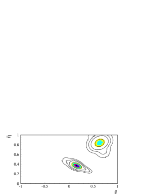
Figure 6: The plot shows the presently allowed probability regions (68$\%$,95$\%$,99$\%$ and 99.9$\%$) in the ($\bar{\rho},\bar{\eta}$) plane using the $(R_{t},\beta)$ strategy: the direct measurement of sin 2$\beta$ and $R_{t}$ from $\Delta M_{d}$ and ${\Delta M_{d}}/{\Delta M_{s}}$

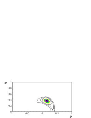
Figure 7: The plot shows the allowed probability regions (68$\%$,95$\%$,99$\%$ and 99.9$\%$) in the ($\bar{\rho},\bar{\eta}$) plane using the $(R_{t},R_{b})$ strategy: $R_{t}$ from $\Delta M_{d}$ and ${\Delta M_{d}}/{\Delta M_{s}}$ and $R_{b}$ from $|V_{ub}/V_{cb}|$

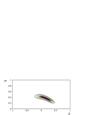
Figure 8: The plot shows the allowed probability regions (68$\%$,95$\%$,99$\%$ and 99.9$\%$) in the ($\bar{\rho},\bar{\eta}$) plane using the $(R_{b},\beta)$ strategy: direct measurement of sin 2$\beta$ and $R_{b}$ from $\left|{V_{ub}}/{V_{cb}}\right|$.

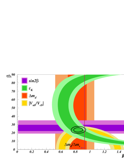
Figure 9: The plot shows the allowed probability regions (68$\%$ and 95$\%$) in the ($R_{t},\beta$) plane. Different constraints are also shown. The line shown for ${\Delta M_{d}}/{\Delta M_{s}}$ constraint corresponds to the 95$\%$ C.L. limit on ${\Delta M_{s}}$

At present the concrete results can be obtained only for the strategies ($R_{t},\beta$), ($R_{b},R_{t}$) and ($R_{b},\beta$) as no direct measurements of $\gamma$ and $\alpha$ are available. The most recent discussions of the strategies for the determination of $\alpha$ and $\gamma$ with the relevant references can be found in [11, 31] and [32].

The results for $\bar{\rho}$ and $\bar{\eta}$ for the three strategies in question are presented in table 2 and in figures 6, 7 and 8. To obtain these results we have used the direct measurement of sin 2$\beta$ [33], $R_{t}$ as extracted from $\Delta M_{d}$ and ${\Delta M_{d}}/{\Delta M_{s}}$ by means of the formulae in [7, 28] and $R_{b}$ as extracted from $|V_{ub}/V_{cb}|$. The experimental and theoretical inputs are summarized in table 1 and the methods are described in [28]. The errors with stars in table 1 are the r.m.s. of the distributions, resulting upon the convolution of the two different determinations, and thus indicative. In the fit full distributions have been used.

It should be emphasized that these three presently available strategies are the weakest among the leading strategies listed in (4.2). Among them $(R_{t},\beta)$ and $(R_{t},R_{b})$ appear to be superior to $(R_{b},\beta)$ at present. We expect that once $\Delta M_{s}$ has been measured and the error on $\sin 2\beta$ reduced, the strategy $(R_{t},\beta)$ will be leading among these three. Therefore in figure 9 we show how the presently available constraints look like in the $(R_{t},\beta)$ plane.

6 An Update on Minimal Flavour Violation Models

The simplest class of extentions of the SM are the models in which only the SM operators in the effective weak Hamiltonian are relevant and in which flavour violation is entirely governed by the CKM matrix. In these models CP violation is governed then solely by the KM phase. The Two-Higgs-Doublet model and the MSSM at low $\tan\beta=v_{2}/v_{1}$ belong to this class of models. We will call this scenario “Minimal Flavour Violation” (MFV) [15] being aware of the fact that for some authors MFV means a more general framework in which also new operators can give significant contributions. See for instance the recent discussions in [39, 40].

The unitarity triangle in specific supersymmetric models of the MFV-type has been extensively analyzed in [16] and general properties of the MFV models have been pointed out in [12, 15, 17, 18, 41, 42, 43]. The interesting virtue of the MFV models is that with respect to $B^{0}_{d,s}-\bar{B}^{0}_{d,s}$ mixings and the CP-violating parameter $\varepsilon_{K}$, they all can be parametrized by a single function $F_{tt}$ [44, 16]. In the SM, $F_{tt}$ results from box diagrams with top quark and $W^{\pm}$ exchanges with $F_{tt}=2.39\pm 0.12$. Beyond the SM, $F_{tt}$ depends on various new parameters like the masses of charginos, squarks and charged Higgs particles and it can in principle take any value.

One of the interesting properties of the MFV models is the existence of the universal unitarity triangle (UUT) [15] that can be constructed from quantities in which all the dependence on new physics cancels out or is negligible like in tree level decays from which $|V_{ub}|$ and $|V_{cb}|$ are extracted. The values of $\bar{\varrho}$, $\bar{\eta}$, $\alpha$, $\beta$, $\gamma$, $R_{b}$, and $R_{t}$ resulting from this determination are the “true” values that are universal within the MFV models. Various strategies for the determination of the UUT are discussed in [15].

The presently available quantities that do not depend on the new physics parameters within the MFV-models and therefore can be used to determine the UUT are $R_{t}$ from $\Delta M_{d}/\Delta M_{s}$ by means of

$$R_{t}=\frac{\xi}{\lambda}\sqrt{\frac{\Delta M_{d}}{\Delta M_{s}}}$$ (6.3)

with $\xi$ defined in table 1, $R_{b}$ from $|V_{ub}/V_{cb}|$ by means of (2.7) and $\sin 2\beta$ extracted from the CP asymmetry in $B^{0}_{d}\to\psi K_{S}$. On the other hand $\varepsilon_{K}$ and $R_{t}$ from $\Delta M_{d}$ alone cannot be used in this construction as they both depend explicitly on $F_{tt}$. Formula (6.3) is an excellent approximation.

Using the necessary input of table 1 that includes the most recent data on $\sin 2\beta$ from BaBar and Belle [33], we find the allowed universal region for $(\bar{\varrho},\bar{\eta})$ in the MFV models shown in figure 10. Similar analysis has been done in [40]. The central values, the errors and the $95\%$ (and $99\%$) probability ranges for various quantities of interest related to this UUT are collected in table 3. These quantities are compared with the corresponding results in the SM as shown in figure 10 and in table 3. To this end all available constraints, that is also $\varepsilon_{K}$ and $\Delta M_{d}$ have been used, following the procedure described in [28]. Other recent analyses of the UT in the SM can be found in [16, 9, 45, 46, 47].

Strategy	UUT	SM
$\bar{\eta}$	0.369 $\pm$ 0.032	0.357 $\pm$ 0.027
	(0.298-0.430) [0.260-0.449]	(0.305-0.411) [0.288-0.427]
$\bar{\rho}$	0.151 $\pm$ 0.057	0.173 $\pm$ 0.046
	(0.034-0.277) [-0.023-0.358]	(0.076-0.260) [0.043-0.291]
$\sin 2\beta$	0.725 ${}^{+0.038}_{-0.028}$	0.725 ${}^{+0.035}_{-0.031}$
	(0.661-0.792) [0.637-0.809]	(0.660-0.789) [0.637-0.807]
$\sin 2\alpha$	0.05 $\pm$ 0.31	-0.09 $\pm$ 0.25
	(-0.62-0.60) [-0.89-0.78]	(-0.54-0.40) [-0.67-0.54]
$\gamma$	67.5 $\pm$ 9.0	63.5 $\pm$ 7.0
(degrees)	(48.2-85.3) [36.5-93.3]	(51.0-79.0) [46.4-83.8]
$R_{b}$	0.404 $\pm$ 0.023	0.400 $\pm$ 0.022
	(0.359-0.450) [0.345-0.463]	(0.357-0.443) [0.343-0.457]
$R_{t}$	0.927 $\pm$ 0.061	0.900 $\pm$ 0.050
	(0.806-1.048) [0.767-1.086]	(0.802-0.998) [0.771-1.029]
$\Delta M_{s}$	17.3${}^{+2.2}_{-1.3}$	18.0${}^{+1.7}_{-1.5}$
($ps^{-1}$)	(15.0-23.0) [11.9-31.9]	(15.4-21.7) [14.8-25.9]
$|V_{td}|~{}(10^{-3})$	8.36 $\pm$ 0.55	8.15 $\pm$ 0.41
	(7.14-9.50) [6.27-10.00]	(7.34-8.97) [7.08-9.22]
$|V_{td}|/|V_{ts}|$	0.209 $\pm$ 0.014	0.205 $\pm$ 0.011
	(0.179-0.238) [0.157-0.252]	(0.184-0.227) [0.177-0.233]
$Im\lambda_{t}$	13.5 $\pm$ 1.2	13.04 $\pm$ 0.94
($10^{-5}$)	(10.9-15.9) [9.4-16.6]	(11.2-14.9) [10.6-15.5]

Table 3: Values and errors for different quantities using the present knowledge summarized in Table 1 for the UUT and the SM Triangle, following the procedure described in [28]. In brackets the 95$\%$ and 99$\%$ probability regions are also given.

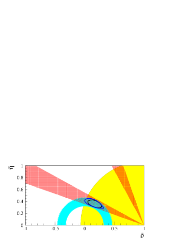
Figure 10: The plot shows the allowed 95$\%$ probability region in the $(\bar{\varrho},\bar{\eta})$ plane, consistent with UUT; the individual 95$\%$ regions for the constraint from $sin2\beta$, $\Delta M_{s}$ and $R_{b}$ are also shown. The narrower region corresponds to the allowed 95$\%$ probability region consistent with SM. The results are obtained using the fit procedure described in [28]

We would like to remark that the measurement $\sin 2\beta=0.734\pm 0.054$ implies two solutions for $\beta$ with $\beta\approx(23.6\pm 2.2)^{\circ}$ and $\beta\approx(66.4\pm 2.2)^{\circ}$. These are shown in fig. 10. In doing this we tacitly assume that the function $F_{tt}$ is positive. Otherwise as discussed in [17] also two solutions with a negative $\beta$ would be possible. As in the SM and in the MFV models there are no new complex phases beyond the CKM phase, the measured $\beta$ is the “true” $\beta$ and not the sum of a true $\beta$ and some additional phase that could be the case in models with additional sources of flavour and CP violation. Consequently by imposing the constraint from $R_{b}$ the solution with the larger $\beta$ can be eliminated for all MFV models resulting in the unique solution with lower $\beta$ as presented in figure 10 and table 3.

It should be stressed that any MFV model that is inconsistent with the broader allowed region in figure 10 and the ”UUT” column in table 3 is ruled out. We observe that there is little room for MFV models that in their predictions differ from the SM as the most ranges within the SM and MFV models do not significantly differ from each other. Among the five observables $R_{t}$, $R_{b}$, $\alpha$, $\beta$ and $\gamma$:

• The allowed ranges for $R_{b}$ and $\beta$ in the SM and general MFV models are essentially indistinguishable from each other.

• On the other hand the allowed ranges for $R_{t}$, $\alpha$ and $\gamma$ in the MFV models are larger than in the SM. Moreover $\Delta M_{s}$ in the MFV models can be slightly larger than in the SM.

Figure 10 and table 3 imply that only certain ranges for the parameters specific to a given MFV model are allowed. We illustrate this with the function $F_{tt}$. Including in our analysis of the MFV models, $\varepsilon_{K}$ and $\Delta M_{d}$ that explicitly depend on $F_{tt}$ [7] we find the range

$$1.3\leq F_{tt}\leq 3.8~{}(95\%~{}{\rm probability~{}region})\qquad[1.2\leq F_{tt}\leq 5.1]~{}(99\%~{}{\rm probability~{}region})$$ (6.4)

This should be compared with the older range $1.2\leq F_{tt}\leq 5.7$ found in [42]. Our results are compatible with those of [16] where specific MFV models have been considered.

The allowed ranges for UUT in figure 10 and table 3 and the range for $F_{tt}$ will be further constrained in the coming years through the improved measurements of $R_{b}$ and $\sin 2\beta$ and in particular of $\Delta M_{s}$.

7 Conclusions

In this paper we have presented a numerical analysis of the unitarity triangle from a different point of view, that emphasizes the role of different strategies in the precise determination of the unitarity triangle parameters. A complete list of the relevant formulae can be found in Section 3. While we have found that the pairs $(\gamma,\beta)$, $(\gamma,R_{b})$ and $(\gamma,\bar{\eta})$ are most efficient in determining $(\bar{\varrho},\bar{\eta})$, we expect that the pair $(R_{t},\beta)$ will play the leading role in the UT fits in the coming years, in particular, when $\Delta M_{s}$ will be measured and the theoretical error on $\xi$ decreased. For this reason we have proposed to plot available constraints on the CKM matrix in the $(R_{t},\beta)$ plane.

It will be interesting to compare in the future the allowed ranges for $(\bar{\varrho},\bar{\eta})$ resulting from different strategies in order to see whether they are compatible with each other. Any discrepancies will signal the physics beyond the SM. We expect that the strategies involving $\gamma$ will play a very important role in this comparison.

For the fundamental set of parameters in the quark flavour physics given in (1.2) we find within the SM

$$|V_{us}|=0.221\pm 0.002,~{}|V_{cb}|=(40.4\pm 0.8)10^{-3},~{}R_{t}=0.90\pm 0.05,~{}\beta=(23.2\pm 1.4)^{\circ}\quad(7.1)$$

where the errors represent one standard deviations and the result for $\beta$ corresponds to $\sin 2\beta=0.725\pm 0.033$.

A complete analysis of the usefulness of a given strategy should also include the discussion of its experimental feasibility and theoretical cleanness. Extensive studies of these two issues can be found in [3, 4, 5, 6, 7]. Again among various strategies, the $(R_{t},\beta)$ strategy is exceptional as the theoretical uncertainties in the determination of these two variables are small and the corresponding experiments are presently feasible. In the long run, when $\gamma$ will be cleanly measured in $B_{s}\to DK$ decays at LHC and constrained through other decays as reviewed in [32] we expect that the strategy $(\gamma,\beta)$ will take over the leading role. Eventually the independent direct determinations of the five variables in question will be crucial for the tests of the SM and its extentions.

We have also determined the universal unitarity triangle for the full class of MFV-models as defined in [15] and we have compared it with the unitarity triangle in the SM. We have found that the allowed ranges for various parameters related to the unitarity triangle do not significantly differ from the ones found in the SM. The result can be found in table 3 and figure 10. The updated $95\%$ probability range for the function $F_{tt}$ that parametrizes different MFV models reads $1.3\leq F_{tt}\leq 3.8$ to be compared with the corresponding range $2.16\leq F_{tt}\leq 2.62$ in the Standard Model.

Acknowledgements

The work has been supported in part by the German Bundesministerium für Bildung und Forschung under the contract 05HT1WOA3 and the DFG Project Bu. 706/1-1.

References

- [1] N. Cabibbo, Phys. Rev. Lett. 10 (1963) 531.
- [2] M. Kobayashi and K. Maskawa, Prog. Theor. Phys. 49 (1973) 652.
- [3] The BaBar Physics Book, eds. P. Harrison and H. Quinn, (1998), SLAC report 504.
- [4] B Decays at the LHC, eds. P. Ball, R. Fleischer, G.F. Tartarelli, P. Vikas and G. Wilkinson, hep-ph/0003238.
- [5] B Physics at the Tevatron, Run II and Beyond, K. Anikeev et al., hep-ph/0201071.
- [6] A.J. Buras and R. Fleischer, Adv. Ser. Direct. High. Energy Phys. 15 (1998) 65; hep-ph/9704376.
- [7] A.J. Buras, hep-ph/0101336, lectures at the International Erice School, August, 2000; Y. Nir, hep-ph/0109090, lectures at 55th Scottish Univ. Summer School, 2001.
- [8] J.M. Soares and L. Wolfenstein, Phys. Rev. D47 (1993) 1021; Y. Nir and U. Sarid, Phys. Rev. D47 (1993) 2818; Y. Grossman and Y. Nir, Phys. Lett. B313 (1993) 126; R. Barbieri, L.J. Hall and A. Romanino, Phys. Lett. B401 (1997) 47; M. Ciuchini, E. Franco, L. Giusti, V. Lubicz and G. Martinelli, Nucl. Phys. B573 (2000) 201-222; P. Paganini, F. Parodi, P. Roudeau and A. Stocchi, Physica Scripta Vol. 58 (1998) 556-569; F. Parodi, P. Roudeau and A. Stocchi Il Nuovo Cimento 112A (1999) 833.
- [9] A. Höcker, H. Lacker, S. Laplace and F. Le Diberder, Eur. Phys. J. C21 (2001) 225.
- [10] G. Buchalla and A.J. Buras, Phys. Rev. D54 (1996) 6782.
- [11] M. Beneke, G. Buchalla, M. Neubert and C.T. Sachrajda, Nucl. Phys. B 606 (2001) 245; M. Gronau and J.L. Rosner, Phys. Rev. D65 (2002) 013004; Z. Luo and J.L. Rosner, Phys. Rev. D54 (2002) 054027.
- [12] A.J. Buras, M.E. Lautenbacher and G. Ostermaier, Phys. Rev. D 50 (1994) 3433.
- [13] A.J. Buras, Phys. Lett. B333 (1994) 476; Nucl. Instr. Meth. A368 (1995) 1.
- [14] R. Aleksan, B. Kayser and D. London, Phys. Rev. Lett. 73 (1994) 18; J.P. Silva and L. Wolfenstein, Phys. Rev. D 55 (1997) 5331; I.I. Bigi and A.I. Sanda, hep-ph/9909479.
- [15] A.J. Buras, P. Gambino, M. Gorbahn, S. Jäger and L. Silvestrini, Phys. Lett. B500 (2001) 161.
- [16] A. Ali and D. London, Eur. Phys. J. C9 (1999) 687; Phys. Rep. 320, (1999), 79; hep-ph/0002167; Eur. Phys. J. C18 (2001) 665.
- [17] A.J. Buras and R. Fleischer, Phys. Rev. D64 (2001) 115010.
- [18] A.J. Buras, P.H. Chankowski, J. Rosiek and Ł. Sławianowska, Nucl. Phys. B 619 (2001) 434.
- [19] G. D’Ambrosio and G. Isidori, Phys. Lett. B530 (2002) 108.
- [20] G.C. Branco, L. Lavoura and J. Silva, (1999), CP Violation, Oxford Science Publications, Clarendon Press, Oxford.
- [21] F.J. Botella, G.C. Branco, M. Nebot and M.N. Rebelo, hep-ph/0206133.
- [22] L.L. Chau and W.-Y. Keung, Phys. Rev. Lett. 53 (1984) 1802.
- [23] Particle Data Group, Euro. Phys. J. C 15 (2000) 1.
- [24] L. Wolfenstein, Phys. Rev. Lett. 51 (1983) 1945.
- [25] M. Schmidtler and K.R. Schubert, Z. Phys. C 53 (1992) 347.
- [26] M. Ciuchini, G. Degrassi, P. Gambino and G.F. Giudice, Nucl. Phys. B 534 (1998) 3.
- [27] T. Goto, N. Kitazawa, Y. Okada and M. Tanaka, Phys. Rev. D53 (1996) 6662. A.G. Cohen, D.B. Kaplan, F. Lepeintre and A.E. Nelson, Phys. Rev. Lett. 78 (1997) 2300. Y. Grossman, Y. Nir and M.P. Worah, Phys. Lett. B407 (1997) 307. G. Barenboim, G. Eyal and Y. Nir, Phys. Rev. Lett. 83 (1999) 4486.
- [28] M. Ciuchini, G. D’Agostini, E. Franco, V. Lubicz, G. Martinelli, F. Parodi, P. Roudeau, A. Stocchi, JHEP 0107(2001) 013 (hep-ph/0012308).
- [29] Belle Collaboration (K. Abe et al.), hep-ex/0204002.
- [30] Talk by A. Farbin (BaBar Collaboration), XXXVIIth Recontres de Moriond, Electroweak Interactions and Unified Theories, Les Arcs, France, 9-16 March 2002, http://moriond.in2p3.fr/EW/2002/.
- [31] R. Fleischer and J. Matias, hep-ph/0204101; M. Gronau and J.L. Rosner, hep-ph/0202170; D. Atwood and A. Soni, hep-ph/0206045; M. Ciuchini, E. Franco, G. Martinelli and L. Silvestrini, Nucl. Phys. B 501 (1997) 271.
- [32] R. Fleischer, hep-ph/0110278 and references therein.
- [33] Average from Y. Nir hep-ph/0208080 based on: R. Barate et al. (ALEPH Collaboration) Phys. Lett. B492 (2000), 259-274; K. Ackerstaff et al. (OPAL Collaboration) Eur. Phys. C5 (1998) 379; T. Affolder at al. Phys. ReV. D61 (2000) 072005; B. Aubert et al. (Babar Collaboration) hep-ex/0207042; K. Abe at al. (Belle Collaboration) hep-ex/0207098.
-
[34]
Results presented at the CKM Unitarity Triangle
Workshop, CERN Feb 2002.
http://ckm-workshop.web.cern.ch/ckm-workshop/
in particular see also :
LEP Working group on : http://lepvcb.web.cern.ch/LEPVCB/ Winter 2002 averages.
LEP Working group on : http://battagl.home.cern.ch/battagl/vub/vub.html. - [35] M. Artuso and E. Barberio, hep-ph/0205163
-
[36]
LEP Working group on oscillations :
http://lepbosc.web.cern.ch/LEPBOSC/combined_results/amsterdam_2002/ - [37] Talk Talk by L. Lellouch, 31st International Conference on High Energy Physics Amsterdam, Amsterdam, Netherland, 24-31 July 2002, http://www.ichep02.nl
-
[38]
F. Abe et al., CDF Collaboration, Phys. Rev. Lett. 74 (1995) 2626;
S. Abachi et al., D0 Collaboration, Phys. Rev. Lett. 74 (1995) 2632. - [39] C. Bobeth, T. Ewerth, F. Krüger and J. Urban, hep-ph/0204225.
- [40] G. D’Ambrosio, G.F. Giudice, G. Isidori and A. Strumia, hep-ph/0207036.
- [41] A.J. Buras and R. Buras, Phys. Lett. 501 (2001) 223.
- [42] S. Bergmann and G. Perez, Phys. Rev. D64 (2001) 115009.
- [43] S. Laplace, Z. Ligeti, Y. Nir and G. Perez, Phys. Rev. D65 (2002) 094040.
- [44] M. Misiak, S. Pokorski and J. Rosiek, hep-ph/9703442, in Heavy Flavours II, eds. A.J. Buras and M. Lindner, World Scientific, 1998, page 795.
- [45] D. Atwood and A. Soni, Phys. Lett. B508 (2001) 17.
- [46] M. Bargiotti et al. Riv. Nuovo Cimento 23N3 (2000) 1.
- [47] A. Stocchi Nucl. Instrum. Meth. A462 (2001) 318-332 and J. Phys. G : Nucl. Part. Phys. 27 (2001) 1101-1109., M. Ciuchini hep-ph/0112133