Saxion Emission from SN1987A

Abstract:

We study the possibility of emission of the saxion, a superpartner of the axion, from SN1987A. The fact that the observed neutrino pulse from SN1987A is in excellent agreement with the current theory of supernovae places a strong bound on the energy loss into any non-standard model channel, therefore enabling bounds to be placed on the decay constant, $f_{a}$, of a light saxion. The low-energy coupling of the saxion, which couples at high energies to the QCD gauge field strength, is expected to be enhanced from QCD scaling, making it interesting to investigate if the saxion could place stronger bounds on $f_{a}$ than the axion itself. Moreover, since the properties of the saxion are determined by $f_{a}$, a constraint on this parameter can be translated into a constraint on the supersymmetry breaking scale. We find that the bound on $f_{a}$ from saxion emission is comparable with the one derived from axion emission due to a cancellation of leading-order terms in the soft-radiation expansion.

1 Introduction

Searches for the neutron electric dipole moment (EDM) $d_{n}$ place strong constraints on the QCD vacuum angle $\theta_{\text{QCD}}$ [1]. The latest incarnation of these experiments gives an upper bound of $|d_{n}|<6.3\times 10^{-26}e$ cm which can be related [2] to the CP-violating parameter in QCD, $\theta_{QCD}$, to give $\theta_{QCD}<(1-10)\times 10^{-10}$. Bounds on $\theta_{QCD}$ coming from ${}^{199}\text{Hg}$ EDM experiments [3] are somewhat stronger, $\theta_{QCD}<1.5\times 10^{-10}$. However, the conversion of the bound on $d(^{199}\text{Hg})$ to a constraint on $\theta_{QCD}$ is model-dependent and subject to large uncertainties.

A possible explanation [4, 5, 6, 7, 8] for the smallness of $\theta_{\text{QCD}}$ is the introduction of a new anomalous global ${U(1)_{\text{PQ}}}$ symmetry which is spontaneously broken at the Peccei-Quinn (PQ) scale ${f_{a}}$. Associated with this spontaneously broken symmetry is a new particle, called the axion [9, 10]. The axion is the pseudo Goldstone boson of the broken PQ symmetry. It develops a mass $m_{a}\simeq m_{\pi}f_{\pi}/f_{a}$ due to the axial anomaly.

The present constraints on $f_{a}$ are $10^{9}~{}\text{GeV}\lesssim{f_{a}}\lesssim 10^{12}~{}\text{GeV}$. The lower bound on the allowed window comes from SN1987A and corresponds to an axion whose coupling is such that it can be abundantly produced in the nascent neutron star and yet interacts weakly enough to allow emission on a similar time scale to the neutrinos. This axion provides a new efficient cooling mechanism and would lead to a shortening of the neutrino pulse from SN1987A, in conflict with observations, if $f_{a}$ is too small [11]. The upper limit on the allowed window comes from cosmological arguments. It corresponds to axions so weakly coupled that they never thermalized in the early universe. At high temperatures the axion field value is misaligned with the value it takes at low temperatures and as the universe cools the axion begins to “roll down” towards its minimum [12]. This leads to coherent oscillations of the axion field. The requirement that the energy density in these oscillations does not overclose the universe leads to the upper bound on ${f_{a}}$.

In this paper we are interested in models which are supersymmetric and use ${U(1)_{\text{PQ}}}$ to solve the strong CP problem. If supersymmetry (SUSY) is combined with ${U(1)_{\text{PQ}}}$ there are superpartners to the axion, which are the fermionic axino and the bosonic saxion. For a given axion model the saxion’s properties are determined by SUSY. In particular, for gauge mediated models [13, 14], the saxion mass $m_{s}$ is comparable to the gravitino mass $m_{3/2}\sim 10^{-2}~{}\text{eV}-1~{}\text{GeV}$. The saxion can be light and could be emitted from the interior of a supernova where the temperature is of order 20 MeV.

We find that the saxion couples in a fashion similar to the dilaton [15]: It couples to the QCD gauge field strength in the ultraviolet (UV) and this coupling is enhanced in the infrared (IR) due to QCD scaling. This enhancement leads to the possibility that astrophysical bounds on $f_{a}$ from the saxion could be stronger than those from the axion. In certain gauge mediated models of SUSY breaking (see [14], for example) the PQ scale, $f_{a}$, is derived from the SUSY breaking parameters. Any constraints on $f_{a}$ can be turned into constraints on these SUSY breaking parameters.

Supernovae (SN), in particular the recent SN1987A, have been used frequently to obtain bounds on new physics using the energy-loss argument. Our current theory of SN explains the shape and duration of SN1987A’s neutrino pulse and is in agreement with the observed data. If there exists a new channel that competes with the neutrinos and transports a comparable amount of energy from the interior of the SN then the current description of SN1987A’s neutrino signal is significantly altered. A criterion for the maximum possible emissivity of a novel energy loss process has been given by Raffelt [11]. It states that the luminosity of the new particle(s) can not exceed the neutrino luminosity of $L_{\nu}\sim 10^{52}$ ergs/s. For a proto-neutron star as developed during SN1987A this criterion translates to an emissivity bound of $\dot{\epsilon}\leq 10^{19}$ ergs/g/s for the new channel, the saxion in our case. Saxion parameters that lead to an emissivity greater than this are ruled out.

Several calculations of axion emissivity from the process $NN\to NNa$ have constrained ${f_{a}}$ [16, 17, 18, 19, 20]. Until recently, the NN scattering amplitude was derived from a one-pion-exchange (OPE) potential. However, as shown in [19], it is possible to relate the amplitude for axion emission to the on-shell NN scattering amplitude which can be derived from the experimentally measured NN scattering data. In contrast to the OPE calculation, this method gives a model-independent result.

Naively one might expect that such a model independent calculation could be repeated for the saxion emission channel $NN\to NNs$. This, however, is not the case due to a cancellation of the leading order terms in the expansion around the soft radiation limit. It is exactly these terms that make a model-independent analysis possible.

In the non-relativistic limit the saxion—being a scalar particle—couples to the nucleon mass. Hence there is no dipole radiation. Axions, on the other hand, couple to spin, which is not conserved in nucleon interactions and therefore they can be emitted by bremsstrahlung. Diagrammatically, the leading order poles corresponding to emission from an external leg sum in the case of axions and cancel in the case of saxions.

For this reason we will calculate the amplitude for saxion emission at tree level in the $SU(3)$ chiral Lagrangian. Using this Lagrangian to model the nucleon-nucleon interaction has several shortcomings, as explained below, and one might doubt the validity of our procedure. However, given the rather large uncertainties in the astrophysical parameters entering the calculation, it gives a sufficient estimate for the emissivity.

We find that saxion emission is comparable to axion emission suggesting that the bound on $f_{a}$ from saxions could be at least as significant as that from axions. However, several simplifying approximations were made in order to carry out the calculation. Once a model-independent calculation becomes feasible it would be interesting to repeat this calculation without relying on these approximations. Including the effects of this previously ignored emission channel could tighten the constraints on the PQ parameter space, if the UV physics is supersymmetric.

This paper is laid out as follows. In Section 2 we derive the properties of the saxion at energies above the SUSY breaking scale. In Section 3 we compute the low energy effective coupling of the saxion. In Section 4 we discuss the soft radiation limit, calculate the saxion emissivity and derive bounds on ${f_{a}}$. We conclude in Section 5.

2 (S)axions

The gauge field piece of the standard model Lagrangian for a theory with a non-zero $\theta_{\text{QCD}}$-angle is

$${\mathcal{L}}=-\frac{1}{2g^{2}}{\text{Tr}}\,F_{\mu\nu}F^{\mu\nu}-\frac{\theta_{\text{QCD}}}{16\pi^{2}}{\text{Tr}}\,F_{\mu\nu}\tilde{F}^{\mu\nu},$$ (1)

where

$$\theta_{\text{QCD}}=\theta+\text{Arg Det}M$$ (2)

and $g$ is the $SU(3)$ gauge coupling constant. Classically, the bare $\theta$ angle can be removed from the QCD Lagrangian by a chiral transformation of the quark fields. However, in the absence of a massless quark, this transformation is no longer a symmetry of the quantum theory since chiral transformations are anomalous. Therefore, $\theta$ gets shifted by chiral phase rotations of the quark fields whereas $\theta_{QCD}$ as defined in Eq. (2) is invariant.

Consistency with experiment requires $\theta_{\text{QCD}}<10^{-9}$. Explaining the smallness of $\theta_{\text{QCD}}$ is the strong $CP$ problem. The PQ solution to the strong $CP$ problem postulates the existence of a new dynamical field, the axion $a$, which allows $\theta_{\text{QCD}}$ to vanish dynamically, $\theta_{\text{QCD}}\rightarrow\theta_{\text{QCD}}+a(x_{\mu})/{f_{a}}$. This is achieved by introducing an anomalous global symmetry $U(1)_{PQ}$ spontaneously broken at the scale $f_{a}$.

Realizing ${U(1)_{\text{PQ}}}$ in a supersymmetric theory necessitates putting the axion in a chiral supermultiplet. This multiplet is filled out by introducing its fermionic partner, the axino, and making the axion $a$ the real part of a complex scalar field. The saxion $s$ is the imaginary part of this scalar field and its couplings are uniquely determined by SUSY from those of the axion.

In a supersymmetric theory the Yang-Mills action is most conveniently written in superspace notation as

$${S}=\frac{1}{8\pi}\text{Im}\,\tau\int d^{4}x\,d^{2}\theta\,{\text{Tr}}\,W^{\alpha}W_{\alpha},$$ (3)

where $\theta$ is a two-component Grassmann variable and $W^{\alpha}$ is a vector superfield which packages the gauge vector field $A_{\mu}$, its superpartner the gaugino, and an auxiliary field. The coupling parameter $\tau$ is chosen as $\tau=\frac{4\pi i}{g^{2}}+\frac{\theta_{\text{QCD}}}{2\pi}$ so that upon expanding Eq. (3) one recovers the terms in Eq. (1). Making $\theta_{\text{QCD}}$ dynamical corresponds to $\tau\rightarrow\tau+\frac{\Phi}{2\pi{f_{a}}}$ where $\Phi$ is a chiral superfield containing the axion, saxion, and axino. Expanding $\Phi$ in terms of its component fields gives a shift of the bosonic piece: $\tau\rightarrow\tau+\frac{1}{2\pi{f_{a}}}(a+is)$. The saxion $s$ couples to $F^{2}$ and the axion $a$ couples to $F\tilde{F}$, as before.

The axion is the pseudo Goldstone boson of ${U(1)_{\text{PQ}}}$; it would be massless were it not for the axial anomaly. Without SUSY the axion gets a vev below the PQ scale and develops a ‘mexican hat’ potential. The radial mode becomes heavy (on the order of the symmetry breaking scale) and the angular mode remains light, becoming the axion. With unbroken SUSY the superpotential is holomorphic and this radial direction remains flat, ignoring the effects of the anomaly. There is now an extra light mode corresponding to oscillations in the radial direction: the saxion. With unbroken SUSY there are two degenerate light modes whose mass is set by the effects of the axial anomaly. Once SUSY is broken this nearly flat direction is lifted and the saxion acquires a mass, independent of the axion. The specifics of the SUSY breaking mechanism determine the form of the potential for $\Phi$ and thus the masses of the saxion and axion. Gauge mediated models predict viable properties for the saxion: Its mass can be light, of ${\mathcal{O}}(10^{-2}\text{eV}-1\text{GeV})$, and $f_{a}$ fits naturally in the allowed window [14, 13].

3 Low Energy Saxion Dynamics

As we run down in energies from above the PQ scale, $f_{a}$, passing the SUSY breaking scale, $M_{\text{SUSY}}$, to below the QCD scale, $\Lambda_{\text{QCD}}$, we pass through various effective theories that describe the relevant degrees of freedom at that energy. Summarizing what was mentioned in the last section ($E\sim\sqrt{q^{2}}$, where $q$ is a typical momentum transfer):

• $E>{f_{a}},\ M_{\text{SUSY}}$: ${U(1)_{\text{PQ}}}$ unbroken, SUSY unbroken.

• $f_{a}>E>M_{\text{SUSY}}$: ${U(1)_{\text{PQ}}}$ broken, SUSY unbroken, degenerate saxion and axion with mass generated by the axial anomaly.

• $M_{\text{SUSY}}>E>\Lambda_{\text{QCD}}$: SUSY broken, superpartners become heavy, nondegenerate massive saxion and axion, quarks and gauge fields are relevant degrees of freedom.

• $\Lambda_{\text{QCD}}>E$: Mesons, baryons, saxion, and axion are relevant degrees of freedom.

The Lagrangian for the saxion-axion system at ${f_{a}}$ is,

$${\mathcal{L}} = \frac{1}{2}(\partial_{\mu}s)^{2}+\frac{1}{2}(\partial_{\mu}a)^{2}-V(a,s)-\left(\frac{1}{2g^{2}}+\frac{1}{16\pi^{2}}\frac{s}{{f_{a}}}\right){\text{Tr}}F^{2}$$ (4)

$$-\frac{1}{16\pi^{2}}\left(\theta_{\text{QCD}}+\frac{a}{{f_{a}}}\right){\text{Tr}}F\tilde{F}+\sum_{i=1}^{6}\left(\bar{q}_{i}i{\hskip 1.79993pt\not{D\hskip 2.70004pt}}q_{i}-m_{i}\bar{q}_{i}q_{i}+\frac{1}{{f_{a}}}\partial_{\mu}a\,\bar{q}_{i}\gamma^{\mu}\gamma_{5}Xq_{i}\right),$$

where the quarks $q_{i}$ have mass $m_{i}$ with the index $i$ running over quark flavors. Furthermore, $V(a,s)$ is undetermined and $X$ is a model dependent flavor mixing matrix.

In order to compute the couplings of the saxion to matter at the low energies typical for neutron stars we need to first integrate out the heavy quarks. We can then match this theory onto a low-energy Lagrangian containing hadrons as the relevant degrees of freedom. The saxion’s interactions can be written in terms of the renormalization group invariant quantities $m_{i}\bar{q}_{i}q_{i}$ and $\partial_{\mu}D^{\mu}$, where the latter is the divergence of the scale current. This method of evaluating the divergence of the scale current in order to calculate matrix elements of the $F^{2}$ operator at low momentum transfer has been developed in [21, 22, 23, 24] and recently applied to systems involving the low energy coupling of the dilaton [15] and quarkonium [25].

At the scale ${f_{a}}$, where the Lagrangian in Eq. (4) is relevant, $\partial_{\mu}D^{\mu}$ is given by

$$\partial_{\mu}D^{\mu}=T^{\mu}_{\mu}=\frac{\beta}{g^{3}}{\text{Tr}}F^{2}+\sum_{i=1}^{6}(1-\gamma_{m_{i}})m_{i}\bar{q}_{i}q_{i}.$$ (5)

Here we have ignored the contributions from the $sF^{2}$ and $aF\tilde{F}$ terms since they are suppressed by a factor of $1/{f_{a}}$ compared to the terms in Eq. (5). Furthermore, $\beta=\partial g/\partial\log\mu$ is the $SU(3)$ beta function for the coupling $g$ given to leading order by $\beta=-b_{0}g^{3}/16\pi^{2}$. Above the SUSY breaking scale $b_{0}$ is given by $b_{0}=9-N_{f}$ for the Minimal Supersymmetric Standard Model. Below the SUSY breaking scale it is given by the standard model result $b_{0}=11-2N_{f}/3$, with $N_{f}$ being the number of flavors. Furthermore, $\gamma_{m_{i}}=\partial m_{i}/\partial\log\mu$ is the mass anomalous dimension. Using Eq. (5) we can rewrite the saxion-gauge field piece of Eq. (4) as,

$${\mathcal{L}}_{s}=\frac{s}{16\pi^{2}{f_{a}}}\frac{g}{\beta}\left(\partial_{\mu}D^{\mu}-\sum_{i=1}^{6}(1-\gamma_{m_{i}})m_{i}\bar{q}_{i}q_{i}\right).$$ (6)

We can now run down in scale from ${f_{a}}$ to $\Lambda_{\text{QCD}}$ via $M_{\text{SUSY}}$, matching across the quark mass thresholds as we go. Working to leading order in $\alpha_{s}=g^{2}/4\pi$ and neglecting $\gamma_{m}$, which is small compared to unity, we arrive at

$${\mathcal{L}}_{s}=\frac{s}{16\pi^{2}{f_{a}}}\kappa\left(\partial_{\mu}D^{\mu}-\sum_{i=1}^{3}m_{i}\bar{q}_{i}q_{i}\right),$$ (7)

where the enhancement factor $\kappa$ is given by

$$\kappa=\frac{4\pi/9}{{\alpha}_{s}(f_{a})}\approx\frac{2}{3}\log\frac{f_{a}}{\text{GeV}}+12.4.$$ (8)

This running gives sizable enhancements to the saxion coupling. For instance, for $f_{a}=10^{9}$ GeV, a SUSY breaking scale of $10^{4}$ GeV, and $\Lambda_{\text{QCD}}=200$ MeV this QCD scaling results in an enhancement of $\kappa\approx 26$ over the naive coupling.

4 Calculating the Emissivity

As detailed in the introduction, the Raffelt criterion limits any mechanism that competes with the neutrinos in removing energy from the neutron star to a maximum emissivity of $10^{19}$ ergs/g/s. The emission of light saxions from the core of the neutron star would provide such an energy-loss mechanism.

Emission rates have been calculated for the emission of other light particles, such as neutrinos ($NN\rightarrow NN\nu\bar{\nu}$) [26, 19], axions ($NN\to NNa$) [19, 16, 17, 18], scalars ($NN\to NNs$) [27], or Kaluza-Klein (KK) gravitons ($NN\rightarrow NNg$) which come about by introducing large gravity-only extra dimensions [28, 29, 30, 31, 32]. There have also been several calculations for the emissivity of these particles where it has been assumed that the relevant degrees of freedom in the core are quarks and gluons, rather than nucleons [33, 34].

In this work we consider a regime with nucleons as the relevant degrees of freedom. In the case of neutrinos, axions, and KK-gravitons it has been possible [19, 30, 31] by using low energy theorems [35, 36] to relate the emission rates for soft emission to the on-shell nucleon-nucleon scattering amplitudes which can be extracted from NN scattering phase-shift data. Such a calculation has the advantage that it is model-independent, which distinguishes it from the often used one-pion-exchange approximation where the nucleon-nucleon amplitude is due only to a single pion exchange. A model-independent calculation is possible for the following reason: If the energy ${\omega}$ of the radiated particle is low compared to the momenta of the nuclei (low radiation limit) then the main contribution to the emissivity comes from bremsstrahlung radiation where the radiated particle couples to an external nucleon line. These processes are ${\mathcal{O}}(1/{\omega})$, they exhibit a $1/\omega$ pole due to an intermediate nucleon being nearly on-shell. The pole amplitude dominates over diagrams where the radiated particle couples to an internal line [which are ${\mathcal{O}}({\omega}^{0})$]. It is this dominance that renders the coupling of the emitted particle to unknown strong interaction vertices subleading and enables the model-independent calculation.

As explained in Section 1, a similar dominance of bremsstrahlung is absent for the saxion process $NN\to NNs$. In each of the four bremsstrahlung-diagrams there is an infrared pole but these cancel in the sum—diagrams where the saxion radiates off one of the internal lines are not suppressed and low energy theorems cannot be constructed for saxion emission.

One way of performing a model-independent calculation would be to use effective field theory (EFT) methods which have seen some advancement in recent years (for a review see, for example, [37]). Moreover, it has been shown by Beane et al. [38] that an expansion of nuclear forces about the chiral limit is formally consistent and seems to converge as suggested by numerical evidence. Beane et al. investigated a toy theory of nucleons interacting with a potential consisting of three Yukawa exchanges ($m_{\rho}=770$ MeV, $m_{\sigma}=500$ MeV, and $m_{\pi}=140$ MeV) where the masses and couplings where chosen in order to reproduce the scattering length and effective range in the ${}^{1}S_{0}$ nucleon-nucleon channel. By treating the pion part of the potential perturbatively (the pion coupling $\bar{\alpha}_{\pi}\propto g_{A}^{2}m_{\pi}^{2}$) this model shows convergence up to nucleon momenta $|\vec{p}|\approx 250$ MeV. While this progress is very encouraging, these methods are not yet developed far enough to be used at momenta $\gtrsim 300$ MeV as are relevant for supernovae. Therefore we will calculate the amplitude for saxion emission in a $SU(3)$ chiral Lagrangian for baryons and the pseudo Goldstone bosons associated with chiral symmetry breaking. OPE models, based on a $SU(2)$ chiral Lagrangian have been used in the past for the case of neutrino, axion, and KK-graviton emission. Although the OPE captures the relevant physics of the nucleon-nucleon interaction in the long distance range, it fails to do so at short distances where the hardcore part of the potential becomes important. Although one may naively think that these contributions are unimportant for nucleon-nucleon interaction at non-relativistic energies, this is not true. Fine-tuning of the underlying parameters renders the short-distance contributions comparable to the long-distance ones.

In cases where it is possible (e.g., axions and neutrinos) to calculate emission rates using both OPE and model-independent techniques, the two methods differ by about a factor of three due to the crude nature of the OPE assertion. We expect our calculation to differ from reality by a similar amount. This is sufficient for our purpose and will not change our conclusions considerably.

Before proceeding we will briefly discuss other saxion emission processes and argue why $NN\to NNs$ is dominant. A possible emission channel is the Compton-like process $P{\gamma}\to Ps$, where $P$ and ${\gamma}$ refer to a proton and photon, respectively. The leading order $1/{\omega}$ piece in this process cancels between the two diagrams with uncrossed and crossed external proton lines and the process contributes at ${\mathcal{O}}({\omega}^{0})$. In addition, this process is suppressed by the fine-structure constant $1/137$ and the proton number fraction $Y_{P}$ in the neutron star which is assumed to be small. Another emission channel, $N\pi\to Ns$, where $\pi$ is either a thermal pion or a pion condensate, starts contributing at ${\mathcal{O}}({\omega}^{0})$ by the same argument. Also, thermal pions, being bosons, obey a Bose-Einstein distribution and their number density is suppressed by $\exp(-m_{\pi}/T)\approx 10^{-3}\dots 10^{-2}$ for $T\approx 20\dots 30$ MeV. The existence of a pion condensate is rather uncertain and as such we will ignore its possible effects. In short, since the saxion-nucleon coupling is a scalar coupling it will commute with every other vertex and hence the $1/{\omega}$ pole will always vanish in the soft-radiation limit.

Before detailing our calculation for $NN\to NNs$, let us point out several effects we have left out in this paper. Throughout the calculation we use in-vacuum amplitudes to calculate processes in a dense medium. Whether this approximation is appropriate has been investigated, for axion emission, in Ref. [39]. It turns out, that high-density effects are significant and can modify the emission rate by a factor of about an order of magnitude.

Next, the emission rate can be suppressed significantly due to multiple-scattering effects as pointed out by Raffelt and Seckel [40]. This effect, which is analogous to the Landau-Pomeranchuk-Migdal (LPM) effect for electromagnetic bremsstrahlung by relativistic electrons, applies if the nucleon collision rate exceeds the oscillation frequency of the emitted radiation. If the time to emit radiation is greater than the time between collisions in the medium then the nucleons will undergo multiple collisions before emission. It is the interference between these collisions that will suppress the radiation. One incorporates this effect be assigning the nucleon a finite decay width, $\Gamma$. This can be done by the following substitution in the squared matrix element:

$$\frac{1}{{\omega}^{2}}\to\frac{1}{{\omega}^{2}+\Gamma^{2}/4}.$$ (9)

A typical width is given by [41]

$$\Gamma=aT^{2}\left[1+\left(\frac{{\omega}}{2\pi T}\right)^{2}\right]$$ (10)

where $a\approx 0.2~{}\text{MeV}^{-1}$. The LPM effect sets in when $\Gamma\approx{\omega}$, or $T\gtrsim 10$ MeV. It suppresses the emission at high temperature, making the late-time cooling phase of the star more important.

For radiation of particles that couple to the spin of the nucleon, such as axions or neutrinos, there is an additional suppression. If the correlation length of the nucleons is small compared to the formation length of the emitted radiation, then the emitted particle couples to an averaged spin since the nucleon-nucleon interaction can flip spin. This averaged spin goes to zero as the nucleon correlation length decreases. For axion emission this effect reduces the limit on $f_{a}$ by about a factor of 2 [42]. The saxion, however, is a scalar and does not couple to the nucleon spin. We therefore expect no suppression of the emissivity due to this effect.

4.1 $SU(3)$ Chiral Lagrangian and Saxion Coupling

For low-momentum processes chiral-perturbation theory is the suitable framework to work in. In contrast to OPE calculations, which are based on $SU(2)$, we use in our calculation a $SU(3)$ chiral Lagrangian. The nucleons in the core of the neutron star have a typical momentum of $\sim 300$ MeV which suggests the inclusion of the strange quark in the calculation. Moreover, as will be explained in more detail below, the strength of the saxion-nucleon coupling depends on the masses of the octet baryons, which necessitates $SU(3)$. As a consequence, at tree-level there are not only $\pi^{0}$ but also $\eta$ exchanges between nucleons.

The strong dynamics of the octets of pseudo Goldstone bosons $M$ and baryon octet $B$ is described, to lowest order, by the Lagrangian

$${\mathcal{L}} = \frac{f^{2}}{8}{\text{Tr}}(\partial_{\mu}\Sigma\,\partial^{\mu}\Sigma^{\dagger})+\lambda\,{\text{Tr}}(m_{q}\Sigma^{\dagger}+\Sigma m_{q}^{\dagger})$$ (11)

$$+{\text{Tr}}B^{\dagger}\left(iD_{0}+\frac{\vec{D}^{2}}{m_{B}}\right)B+D\,{\text{Tr}}B^{\dagger}\sigma^{i}\{A_{i},B\}+F\,{\text{Tr}}B^{\dagger}\sigma^{i}[A_{i},B]$$

where $D_{\mu}=\partial_{\mu}+V_{\mu}$ and $m_{q}$ is the quark mass matrix $m_{q}=\text{diag}(m_{u},m_{d},m_{s})$. Furthermore

$$\Sigma = \exp\left(\frac{2iM}{f}\right),\hskip 28.45274pt\Sigma=\xi^{2},\hskip 28.45274ptM=\frac{1}{\sqrt{2}}\lambda^{\alpha}\pi^{\alpha},$$

$$V_{\mu} = \frac{1}{2}\left(\xi^{\dagger}\partial_{\mu}\xi+\xi\partial_{\mu}\xi^{\dagger}\right),\hskip 28.45274ptA_{\mu}=\frac{i}{2}\left(\xi\partial_{\mu}\xi^{\dagger}-\xi^{\dagger}\partial_{\mu}\xi\right),$$ (12)

and the $\lambda^{\alpha}$ are the $SU(3)$ generators. We use the convention where the decay constant $f=132$ MeV.

The proton number fraction $Y_{p}$ is typically small in SN, especially during later times in the SN’s evolution when most of the protons have neutronized. Therefore, and in order to unclutter our formulae, we specialize our treatment at this point to $nn$ scattering by taking $Y_{p}=0$. Although we could carry out the calculation for the general case of a proto-neutron plasma specified by $Y_{p}$, we expect the inclusions of protons to make little difference in our result.

To lowest order in the chiral expansion, the contributing diagrams are those where a single $\pi^{0}$ or $\eta$ is being exchanged between two neutron lines. Therefore, we need to just keep neutrons $n$ as well as $\pi^{0}$ and $\eta$. Then the Lagrangian in Eq. (11) reduces to

$${\mathcal{L}} = n^{\dagger}(i\partial_{0}+\frac{\vec{\nabla}^{2}}{2M_{n}})n-g_{\pi}n^{\dagger}\vec{\sigma}\cdot\vec{\nabla}\pi^{0}\,n-g_{\eta}n^{\dagger}\vec{\sigma}\cdot\vec{\nabla}\eta\,n$$ (13)

$$+\frac{1}{2}\partial_{\mu}\pi^{0}\partial^{\mu}\pi^{0}-\frac{m_{\pi}^{2}}{2}(\pi^{0})^{2}+\frac{1}{2}\partial_{\mu}\eta\partial^{\mu}\eta-\frac{m_{\eta}^{2}}{2}\eta^{2},$$

where $n$ is the neutron 2-spinor and $M_{n}$ is the mass of the neutron. The couplings of neutrons to $\pi^{0}$ and $\eta$ are

$$g_{\pi}=\frac{D+F}{\sqrt{2}f},\quad g_{\eta}=\frac{D-3F}{\sqrt{6}f}.$$ (14)

Note that the $V_{\mu}$ coupling has disappeared as it involves a baryon-baryon-pion-pion coupling which does not contribute to saxion emission at tree-level. The meson masses can be calculated in terms of the quark masses,

$$m_{\pi}^{2}=\frac{4\lambda}{f^{2}}(m_{u}+m_{d}),\quad m_{\eta}^{2}=\frac{4\lambda}{f^{2}}\frac{m_{u}+m_{d}+4m_{s}}{3}.$$ (15)

The parameters $D$ and $F$ can be determined from fitting to the measured hyperon semileptonic decays. This has been done by several authors [43, 44, 45, 46, 47]. At tree level a typical fit gives $D=0.79\pm 0.10$ and $F=0.47\pm 0.07$, where the errors are highly correlated, resulting in the combinations $D+F=1.26\pm 0.08$ and $3F-D=0.65\pm 0.21$ [45]. If one includes chiral loop corrections, which are ${\mathcal{O}}(m_{s}\ln m_{s})$, a typical best fit gives $D=0.64\pm 0.06$ and $F=0.34\pm 0.04$ [45], where intermediate decuplet baryons have been included. For our tree level calculation we use typical values of $D=0.8$ and $F=0.5$.

To calculate the coupling of saxions to $n$, $\pi^{0}$ and $\eta$ from the Lagrangian in Eq. (6) we first need to calculate the trace of the energy-momentum tensor $T_{\mu\nu}$ from Eq. (11). Making use of the equation of motion for neutrons, we find

$$\partial_{\mu}D^{\mu}=T^{\mu}_{\mu}=M_{n}\bar{n}n+2m_{\pi}^{2}{\pi^{0}}^{2}-(\partial_{\mu}\pi^{0})^{2}+2m_{\eta}^{2}{\eta}^{2}-(\partial_{\mu}\eta)^{2}.$$ (16)

Since the saxion couples to $\partial_{\mu}D^{\mu}-\sum_{i=1}^{3}m_{i}\bar{q_{i}}q_{i}$ we need to calculate the matrix elements of this operator sandwiched between our low-energy degrees of freedom, neutrons, $\pi^{0}$, and $\eta$. Matching

$$\sum_{i=1}^{3}m_{i}\bar{q_{i}}q_{i}\longrightarrow-\lambda{\text{Tr}}(m_{q}\Sigma^{\dagger}+m_{q}\Sigma)=\frac{m_{\pi}^{2}}{2}(\pi^{0})^{2}+\frac{m_{\eta}^{2}}{2}\eta^{2}$$ (17)

we get

$$\langle\pi^{0}(q^{\prime})|\partial_{\mu}D^{\mu}-\sum_{i=1}^{3}m_{i}\bar{q_{i}}q_{i}|\pi^{0}(q)\rangle=-2q^{\prime}\cdot q+3m_{\pi}^{2}$$ (18)

and

$$\langle\eta(q^{\prime})|\partial_{\mu}D^{\mu}-\sum_{i=1}^{3}m_{i}\bar{q_{i}}q_{i}|\eta(q)\rangle=-2q^{\prime}\cdot q+3m_{\eta}^{2}.$$ (19)

Similarly we obtain for the neutrons $n$

$$\langle n(p)|\partial_{\mu}D^{\mu}-\sum_{i=1}^{3}m_{i}\bar{q_{i}}q_{i}|n(q)\rangle=\tilde{M}$$ (20)

where $\tilde{M}=687\pm 75$ MeV [48, 15] and can be calculated from the masses of the octet baryons and the pion-nucleon $\Sigma$-term. The error for $\tilde{M}$ stems from an estimated 30% error typical for $SU(3)$ violation. Finally, the couplings of the saxion to the nucleon-pion and nucleon-eta vertices vanish,

$$\langle n(p^{\prime})\pi^{0}(q)|\partial_{\mu}D^{\mu}-\sum_{i=1}^{3}m_{i}\bar{q_{i}}q_{i}|n(p)\rangle=\langle n(p^{\prime})\eta(q)|\partial_{\mu}D^{\mu}-\sum_{i=1}^{3}m_{i}\bar{q_{i}}q_{i}|n(p)\rangle=0.$$ (21)

Putting these interactions into the saxion Lagrangian [Eq. (7)] we arrive at

$${\mathcal{L}}_{s}=\frac{\kappa}{16\pi^{2}f_{a}}\left(\tilde{M}sn^{\dagger}n+\frac{3}{2}m_{\pi}^{2}s(\pi^{0})^{2}-s(\partial_{\mu}\pi^{0})^{2}+\frac{3}{2}m_{\eta}^{2}s\eta^{2}-s(\partial_{\mu}\eta)^{2}\right).$$ (22)

Before calculating the saxion emission amplitude in detail using the chiral Lagrangian and saxion coupling given above, we will do a comparison between the cross sections for saxions and axions in nuclear matter based on dimensional arguments.

4.2 Comparison between Saxion and Axion Emissivity

The coupling of axions to nucleons is given by

$$\frac{1}{f_{a}}N^{\dagger}\vec{\sigma}\cdot\vec{\nabla}a\,N$$ (23)

so that the lowest order in the ${\omega}$ expansion of the cross section for $NN\to NNa$ goes like

$$\sigma_{a}\sim\frac{1}{f_{a}^{2}}\frac{{\omega}^{2}}{\Lambda_{\text{QCD}}^{2}}\left(\frac{M_{n}}{{\omega}}\right)^{2}.$$ (24)

Here, the $(M_{n}/\omega)^{2}$ term is due to the $1/{\omega}$ pole coming from a nearly on-shell intermediate nucleon. Using the Lagrangian for the coupling of the saxion to nucleons given in Eq. (6) we can write a similar cross section for $NN\to NNs$:

$$\sigma_{s}\sim\frac{\kappa^{2}}{(16\pi^{2})^{2}f_{a}^{2}}\frac{\tilde{M}^{2}}{\Lambda_{\text{QCD}}^{2}}.$$ (25)

Now, because of the aforementioned $1/{\omega}$ pole cancellation in the case of the saxion, the piece of lowest order in $\omega$ is ${\mathcal{O}}({\omega}^{0})$. Comparing the expected saxion and axion emissivities we find

$$\frac{\dot{{\epsilon}}_{s}}{\dot{{\epsilon}}_{a}}\sim\frac{\kappa^{2}\tilde{M}^{2}}{256\pi^{4}M_{n}^{2}}\simeq 10^{-2}.$$ (26)

So on dimensional grounds we expect the saxion emissivity to be suppressed be about 2 orders of magnitude compared to the axion emissivity.

4.3 Matrix Element

The relevant saxion emission processes are shown in Fig. 1. There is a total of 16 bremsstrahlung-type diagrams (4 direct and 4 crossed pion exchanges, 8 eta exchanges) [referred to as type (a) diagrams]. Moreover, there are 4 diagrams where the saxion couples to the exchanged meson [type (c)]. The type (b) diagrams do not contribute.

Figure 1: The three types of diagrams for the process $nn\rightarrow nns$. Including crossings, there are 16 diagrams (8 pion and 8 eta exchanges) of the type shown in panel (a), 4 diagrams of type (c), and no contribution from type (b) diagrams. A solid circle denotes a meson-nucleon-nucleon vertex, while a solid (empty) square denotes the coupling of the saxion to a nucleon (meson) line. The saxion coupling to the meson-nucleon-nucleon vertex is denoted by an empty circle. A dashed line denotes either $\pi^{0}$ or $\eta$.

As an example, the diagram pictured in Fig. 1(a), where the exchanged meson is the $\pi^{0}$, gives a contribution of

$$\frac{-i\kappa\tilde{M}g_{\pi}^{2}}{16\pi^{2}f_{a}}(p_{4}-p_{2})_{i}(p_{4}-p_{2})_{j}\left[\frac{1}{2E_{3}}\left(\frac{M+E_{3}}{{\omega}}+1\right)\right]\frac{1}{(p_{4}-p_{2})^{2}-m_{\pi}^{2}}n^{\dagger}_{3}\sigma^{i}n_{1}\,n^{\dagger}_{4}\sigma^{j}n_{2}.$$ (27)

Similarly, the diagram depicted in Fig. 1(c) for the $\pi^{0}$ exchange contributes

$$\frac{-i\kappa g_{\pi}^{2}}{16\pi^{2}f_{a}}(p_{1}-p_{3})_{i}(p_{4}-p_{2})_{j}\frac{1}{(p_{1}-p_{3})^{2}-m_{\pi}^{2}}\frac{1}{(p_{2}-p_{4})^{2}-m_{\pi}^{2}}$$

$$\phantom{asdfasdfasfasfasasdfasdffasf}\times\left[3m_{\pi}^{2}-2(p_{1}-p_{3})(p_{4}-p_{2})\right]n^{\dagger}_{3}\sigma^{i}n_{1}\,n^{\dagger}_{4}\sigma^{j}n_{2}.$$ (28)

Here, $\sigma_{i}$ are the Pauli matrices and $E_{i}=M+\vec{p_{i}}^{2}/2M$ in the non-relativistic approximation. Note that in Eq. (27) we need to keep terms up to ${\cal O}({\omega}^{0})$. These will become the main contribution from the type (a) diagrams as the pole drops out.

The squared amplitude can then be calculated after summing over spins in terms of the 4-momenta $k=p_{2}-p_{4}$ and $l=p_{2}-p_{3}$ and is found to be

$$|{\cal M}|^{2} = \sum_{\text{spins}}|{\cal M}_{(a)}+{\cal M}_{(b)}+{\cal M}_{(c)}|^{2}$$ (29)

$$= \frac{\kappa^{2}M^{4}}{4\pi^{4}f_{a}^{2}}\left\{(K_{1}+K_{2})^{2}k^{4}+(L_{1}+L_{2})^{2}l^{4}-(K_{1}+K_{2})(L_{1}+L_{2})(2[k\cdot l]^{2}-k^{2}l^{2})\right\}$$

where

$$K_{1}=\frac{2\tilde{M}}{E_{CM}}\left(\frac{g_{\pi}^{2}}{k^{2}-m_{\pi}^{2}}+\frac{g_{\eta}^{2}}{k^{2}-m_{\eta}^{2}}\right),$$ (30)

$$K_{2}=\frac{g_{\pi}^{2}(3m_{\pi}^{2}-2k^{2})}{(k^{2}-m_{\pi}^{2})^{2}}+\frac{g_{\eta}^{2}(3m_{\eta}^{2}-2k^{2})}{(k^{2}-m_{\eta}^{2})^{2}}$$ (31)

and $L_{1}$ and $L_{2}$ are defined analogously with $k\rightarrow l$.

In this calculation we have assumed the mass of the saxion $m_{s}$ to be small compared to the nucleon momenta and have neglected it.

4.4 Phase-space integration

In order to calculate the emissivity due to saxion $s$ radiation from the two-body scattering reaction $a+b\rightarrow a+b+s$ in neutron matter, where the labels $a$ and $b$ represent a neutron, we have to integrate over the phase space of incoming ($\vec{p_{1}}$, $\vec{p_{2}}$) and outgoing ($\vec{p_{3}}$, $\vec{p_{4}}$) nucleons as well as that of the emitted saxion ($\vec{k_{s}}$). The formula for the emissivity is

$$\frac{d{\cal E}_{X}}{dt} = \int\left[\prod_{i=1..4}\frac{d^{3}p_{i}}{(2\pi)^{3}2E_{i}}\right]\int\frac{d^{3}k_{s}}{(2\pi)^{3}2\omega}f_{1}f_{2}(1-f_{3})(1-f_{4})$$ (32)

$$\times(2\pi)^{4}\delta^{4}(p_{1}+p_{2}-p_{3}-p_{4}-k)S\omega|{\mathcal{M}}|^{2}$$

where the functions $f_{i}$ are Pauli blocking factors given by $f_{i}=(\exp[(E_{i}-\mu)/T]+1)^{-1}$ and $S=1/4$ is the symmetry factor for $nn$ scattering.

In the soft-radiation limit we can neglect the saxion momentum $\vec{k_{s}}$ in the momentum-conserving delta function. Furthermore, by introducing the total momentum $\vec{P}=\vec{p_{1}}+\vec{p_{2}}=\vec{p_{3}}+\vec{p_{4}}$ we can reduce the number of integrations by exploiting spherical symmetry and momentum conservation to obtain

$$\frac{d{\cal E}_{X}}{dt} = \frac{1}{2^{16}\pi^{8}}\int_{0}^{\infty}dP\,|\vec{P}|^{2}\int_{0}^{\infty}dk\,|\vec{k}|^{2}\int_{0}^{\infty}dl\,|\vec{l}|^{2}\int_{-1}^{1}d\cos\theta_{k}\int_{-1}^{1}d\cos\theta_{l}\int_{0}^{2\pi}d\phi$$ (33)

$$\times\frac{\omega^{2}}{E_{1}E_{2}E_{3}E_{4}}f_{1}f_{2}(1-f_{3})(1-f_{4})|{\mathcal{M}}|^{2}.$$

The angles $\theta_{k}$ and $\theta_{l}$ are defined by $\vec{k}\cdot\vec{P}=|\vec{k}||\vec{P}|\cos\theta_{k}$ and $\vec{l}\cdot\vec{P}=|\vec{l}||\vec{P}|\cos\theta_{l}$, while $\phi$ is the angle between the projections of $\vec{k}$ and $\vec{l}$ onto the $\hat{P}$-plane and is given by

$$\cos{\theta_{\mbox{cm}}}=\cos\phi\sin\theta_{k}\sin\theta_{l}+\cos\theta_{k}\cos\theta_{l}$$ (34)

where $\cos{\theta_{\mbox{cm}}}$ is the center of momentum (COM) scattering angle. Also, ${\omega}$ is constrained by the energy delta function to be ${\omega}=E_{1}+E_{2}-E_{3}-E_{4}$.

The expression in Eq. (33) is valid for all temperatures and chemical potentials. In the general regime it must be evaluated numerically.

The result simplifies significantly if one assumes either a degenerate or a highly non-degenerate neutron gas in the star. Although nuclear matter at densities of a few times nuclear matter density and a temperature of $10-50$ MeV is neither degenerate nor non-degenerate, it is nevertheless instructive to calculate saxion emissivity in these two limits.

4.5 Limiting Case: Degenerate Neutron Gas

For a degenerate neutron gas one can assume that saxion radiation only arises from scattering involving neutrons near the Fermi surface in the initial and final states. Assuming soft radiation the momentum $|\vec{p_{i}}|$ of the neutrons in Eq. (32) can be set to $p_{F}$ causing a decoupling of the energy and angular integrations:

$$\frac{d{\cal E}_{X}}{dt} = \frac{p_{F}^{4}}{2^{16}\pi^{10}}\int_{0}^{\infty}d{\omega}\,{\omega}^{2}\int dE_{1}dE_{2}dE_{3}dE_{4}\,{\delta}(E_{1}+E_{2}-E_{3}-E_{4}-{\omega})f_{1}f_{2}(1-f_{3})(1-f_{4})$$ (35)

$$\times\int d{\Omega}_{1}d{\Omega}_{2}d{\Omega}_{3}d{\Omega}_{4}{\delta}^{3}(\vec{p_{1}}+\vec{p_{2}}-\vec{p_{3}}-\vec{p_{4}})|{\mathcal{M}}|^{2}$$

where the ${\delta}{\Omega}_{i}$ is the angular integration of the $\vec{p_{i}}$.

Carrying out the energy [49, 50] and angular integrations one finally integrates over ${\omega}$ to find

$$\frac{d{\cal E}_{X}}{dt}=\frac{31}{2^{12}945\pi^{2}}p_{F}T^{6}\int_{0}^{\pi}d{\alpha}\,\sin{\alpha}\int_{0}^{2\pi}d{\theta_{\mbox{cm}}}|{\cal M}|^{2},$$ (36)

where $\cos{{\alpha}}=\vec{P}\cdot\vec{p_{1}}/|\vec{P}||\vec{p_{1}}|$. The COM scattering angle ${\theta_{\mbox{cm}}}$ is the angle between the projections of $\vec{p_{1}}$ and $\vec{p_{3}}$ into the $\vec{P}$ plane.

4.6 Limiting Case: Non-Degenerate Neutron Gas

In the limit where the system can be treated as a non-degenerate system the initial-state distributions become (non-relativistic) Maxwell-Boltzmann distributions,

$$f_{i}(\vec{p_{i}})=\frac{n}{2}\left(\frac{2\pi}{MT}\right)^{3/2}\exp\left(-\frac{|\vec{p_{i}}|^{2}}{2MT}\right)\quad\text{for}\quad i=1,2$$ (37)

where

$$n=2\int\frac{d^{3}p}{(2\pi)^{3}}\,f_{i}(\vec{p_{i}})$$ (38)

is the neutron number density and the factor of 2 is for the two spin states of neutrons. The final-state blocking factors can be set to unity since basically the complete final-state phase space is available. Then, starting from Eq. (33), the integration over $P$ can be done analytically, leaving

$$\frac{d{\cal E}_{X}}{dt} = \frac{n^{2}}{2^{14}\pi^{9/2}}T^{-3/2}M^{-15/2}\int_{0}^{\infty}dk\int_{0}^{\infty}dl\int_{-1}^{1}d\cos\theta_{k}\int_{-1}^{1}d\cos\theta_{l}\int_{0}^{2\pi}d\phi$$ (39)

$$\phantom{sffhfhff}\times|\vec{k}|^{4}|\vec{l}|^{4}\cos^{2}\theta_{kl}\exp\left(-\frac{|\vec{k}|^{2}+|\vec{l}|^{2}+2|\vec{k}||\vec{l}|\cos\theta_{kl}}{4MT}\right)|{\mathcal{M}}|^{2}.$$

4.7 Numerical Results

We show in Fig. 2 the emissivity for nuclear density $n=n_{0}$, where $n_{0}=0.17\,\text{fm}^{-3}=1.36\cdot 10^{6}\,\text{MeV}^{3}$, and varying temperature including the limiting cases of degenerate and non-degenerate matter. In the figure we have set ${f_{a}}=1$ GeV and $\kappa=1$.

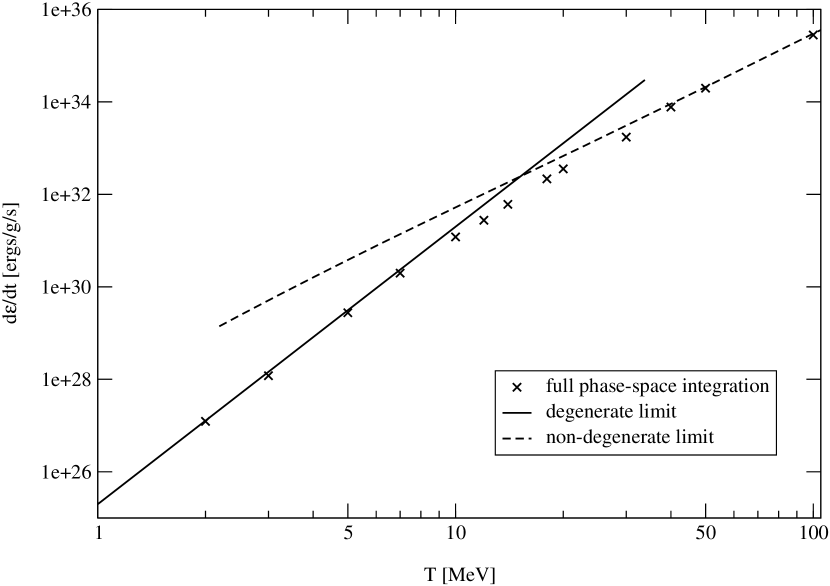
Figure 2: Saxion emissivity for fixed $f_{a}=1$ GeV, $\kappa=1$ at nuclear matter density depending on temperature. The crosses are values from the full phase-space integration, the solid and dashed lines denote the result from the degenerate and non-degenerate matter calculations.

As expected, the degenerate approximation is good at low temperature while the non-degenerate one is better suited to a high temperature regime.

For a typical temperature of $T=20$ MeV and $n=n_{0}$ the emissivity is given by

$$\dot{{\epsilon}}\approx\kappa^{2}\left(\frac{\text{GeV}}{f_{a}}\right)^{2}3.5\times 10^{32}\frac{\text{erg}}{\text{g}\cdot\text{s}}$$ (40)

so that, upon using Raffelt’s criterion of $10^{19}\,\text{ergs/g/s}$ and Eq. (8), we can solve for the PQ scale $f_{a}$ which gives a bound of

$$f_{a}\gtrsim 1.5\times 10^{8}\,\text{GeV}$$ (41)

that is close to the bound of $10^{9}$ GeV coming from the axion. However, if the temperature in the neutron star is as high as 50 MeV the same calculation gives a bound as strong as that from axion emission.

The inclusion of the $\eta$, typically absent in OPE calculations, increases the emissivity by only about 10% because it is four times as heavy as the pion. Furthermore, we expect the LPM effect to weaken our bound for $T=20$ MeV by a factor of $\sim 5$.

5 Conclusions

If both PQ symmetry and SUSY are realized in nature, a new scalar particle, called the saxion, is introduced as a supersymmetric partner of the axion. The properties of the saxion are determined uniquely by SUSY and linked to those of the axion. Both particles, if they exist and are light, are produced in SN. In the past, several calculations using the energy-loss argument for the axion have been made in order to place bounds on the PQ scale ${f_{a}}$. In this paper we used saxion emission to bound $f_{a}$.

The fact that the axion couples to ${\text{Tr}}F\tilde{F}$ while the saxion couples to ${\text{Tr}}F^{2}$ at an energy scale of $f_{a}$ causes the two particles to couple very differently to nucleons at energies typical to neutron stars. In the limit that there is a massless quark the strong CP problem disappears and there is no need for an axion. Hence, for a quark mass approaching zero the axion-nucleon coupling goes to zero. In the same limit, however, the saxion does not decouple since it couples to the QCD field strength. One might therefore expect that the saxion coupling is enhanced over the axion coupling. There is also the added effect of enhancement due to QCD scaling in the case of the saxion. On the other hand, saxion emission is suppressed because the $1/{\omega}$ pole, which is present for the axion, is absent. Thus it is not clear a priori how the bounds on $f_{a}$ coming from the two particles compare.

Ideally one would like to repeat the model-independent calculation of the axion emissivity [19] for the saxion. This turns out not to be possible because the $1/{\omega}$ pole is not present. Therefore, low energy theorems, which enable one to relate the emissivity to the on-shell nucleon-nucleon scattering amplitudes are no longer applicable and one is forced to confront the full details of the nucleon-nucleon strong interaction.

In the past the nucleon-nucleon potential has frequently been approximated by an OPE. This OPE approximation is of a crude nature since it misses short-distance physics which is more important than one might naively expect. Therefore its validity is difficult to quantify. However, in the case of neutrino and axion emission comparisons of the OPE approximation with a model-independent calculation have shown that, surprisingly, the two methods give similar results to within about a factor of three. In our calculation of saxion emission we used an $SU(3)$ chiral Lagrangian, calculating the cross section to tree-level. Since this method is closely related to the OPE approximation, one might hope that it does equally well.

Combining our result for saxion emission with the Raffelt criterion we find a bound on $f_{a}$ that is very close to the one coming from axion emission. In view of the significant amount of uncertainty in our calculation this raises the possibility that saxion emission could significantly raise the lower bound on $f_{a}$. We hope that the exciting prospect of further tightening the bound on $f_{a}$ gives motivation to a model-independent repetition of our calculation once the necessary EFT tools become available.

- [1] P. G. Harris et. al., New experimental limit on the electric dipole moment of the neutron, Phys. Rev. Lett. 82 (1999) 904–907.
- [2] R. J. Crewther, P. Di Vecchia, G. Veneziano, and E. Witten, Chiral estimate of the electric dipole moment of the neutron in quantum chromodynamics, Phys. Lett. B88 (1979) 123.
- [3] M. V. Romalis, W. C. Griffith, and E. N. Fortson, A new limit on the permanent electric dipole moment of hg- 199, Phys. Rev. Lett. 86 (2001) 2505–2508, [http://arXiv.org/abs/hep-ex/0012001].
- [4] R. D. Peccei and H. R. Quinn, Cp conservation in the presence of instantons, Phys. Rev. Lett. 38 (1977) 1440–1443.
- [5] R. D. Peccei and H. R. Quinn, Constraints imposed by cp conservation in the presence of instantons, Phys. Rev. D16 (1977) 1791–1797.
- [6] M. Dine, W. Fischler, and M. Srednicki, A simple solution to the strong cp problem with a harmless axion, Phys. Lett. B104 (1981) 199.
- [7] J. E. Kim, Weak interaction singlet and strong cp invariance, Phys. Rev. Lett. 43 (1979) 103.
- [8] M. A. Shifman, A. I. Vainshtein, and V. I. Zakharov, Can confinement ensure natural cp invariance of strong interactions?, Nucl. Phys. B166 (1980) 493.
- [9] S. Weinberg, A new light boson?, Phys. Rev. Lett. 40 (1978) 223–226.
- [10] F. Wilczek, Problem of strong p and t invariance in the presence of instantons, Phys. Rev. Lett. 40 (1978) 279–282.
- [11] G. G. Raffelt, Stars as laboratories for fundamental physics: The astrophysics of neutrinos, axions, and other weakly interacting particles. The University of Chicago Press, Chicago & London, 1996.
- [12] E. W. Kolb and M. S. Turner, The Early Universe. Addison-Wesley, Redwood City, USA, 1990.
- [13] T. Asaka and M. Yamaguchi, Hadronic axion model in gauge-mediated supersymmetry breaking, Phys. Lett. B437 (1998) 51–61, [http://arXiv.org/abs/hep-ph/9805449].
- [14] T. Asaka and M. Yamaguchi, Hadronic axion model in gauge-mediated supersymmetry breaking and cosmology of saxion, Phys. Rev. D59 (1999) 125003, [http://arXiv.org/abs/hep-ph/9811451].
- [15] D. B. Kaplan and M. B. Wise, Couplings of a light dilaton and violations of the equivalence principle, JHEP 08 (2000) 037, [http://arXiv.org/abs/hep-ph/0008116].
- [16] N. Iwamoto, Axion emission from neutron stars, Phys. Rev. Lett. 53 (1984) 1198–1201.
- [17] R. P. Brinkmann and M. S. Turner, Numerical rates for nucleon-nucleon axion bremsstrahlung, Phys. Rev. D38 (1988) 2338.
- [18] A. Burrows, M. S. Turner, and R. P. Brinkmann, Axions and sn1987a, Phys. Rev. D39 (1989) 1020.
- [19] C. Hanhart, D. R. Phillips, and S. Reddy, Neutrino and axion emissivities of neutron stars from nucleon nucleon scattering data, Phys. Lett. B499 (2001) 9–15, [http://arXiv.org/abs/astro-ph/0003445].
- [20] N. Iwamoto, Nucleon-nucleon bremsstrahlung of axions and pseudoscalar particles from neutron star matter, Phys. Rev. D64 (2001) 043002.
- [21] M. A. Shifman, A. I. Vainshtein, and V. I. Zakharov, Remarks on higgs - boson interactions with nucleons, Phys. Lett. B78 (1978) 443.
- [22] M. B. Voloshin, Trace anomaly in qcd and processes with a light higgs boson, Sov. J. Nucl. Phys. 45 (1987) 122.
- [23] R. S. Chivukula, A. G. Cohen, H. Georgi, and A. V. Manohar, Couplings of a light higgs boson, Phys. Lett. B222 (1989) 258–262.
- [24] R. S. Chivukula, A. G. Cohen, H. Georgi, B. Grinstein, and A. V. Manohar, Higgs decay into goldstone bosons, Annals Phys. 192 (1989) 93–103.
- [25] J.-W. Chen and M. J. Savage, Hadronic and electromagnetic interactions of quarkonia, Phys. Rev. D57 (1998) 2837–2846, [http://arXiv.org/abs/hep-ph/9710338].
- [26] B. L. Friman and O. V. Maxwell, Neutron star neutrino emissivities, . Nordita Copenhagen - NORDITA-78-15 (78,REC.JUN) 86p.
- [27] N. Ishizuka and M. Yoshimura, Axion and dilaton emissivity from nascent neutron stars, Prog. Theor. Phys. 84 (1990) 233–250.
- [28] S. Cullen and M. Perelstein, Sn1987a constraints on large compact dimensions, Phys. Rev. Lett. 83 (1999) 268–271, [http://arXiv.org/abs/hep-ph/9903422].
- [29] V. D. Barger, T. Han, C. Kao, and R.-J. Zhang, Astrophysical constraints on large extra dimensions, Phys. Lett. B461 (1999) 34–42, [http://arXiv.org/abs/hep-ph/9905474].
- [30] C. Hanhart, D. R. Phillips, S. Reddy, and M. J. Savage, Extra dimensions, sn1987a, and nucleon nucleon scattering data, Nucl. Phys. B595 (2001) 335–359, [http://arXiv.org/abs/nucl-th/0007016].
- [31] C. Hanhart, J. A. Pons, D. R. Phillips, and S. Reddy, The likelihood of gods’ existence: Improving the sn 1987a constraint on the size of large compact dimensions, Phys. Lett. B509 (2001) 1–9, [http://arXiv.org/abs/astro-ph/0102063].
- [32] P. J. Fox, Weakly warped extra dimensions and sn1987a, JHEP 02 (2001) 022, [http://arXiv.org/abs/hep-ph/0012165].
- [33] N. Iwamoto, Neutrino emissivities and mean free paths of degenerate quark matter, Annals of Physics 141 (1982) 1–49.
- [34] D. Arndt, How a quark-gluon plasma phase modifies the bounds on extra dimensions from sn1987a, Nucl. Phys. B612 (2001) 171–190, [http://arXiv.org/abs/nucl-th/0102040].
- [35] F. E. Low, Bremsstrahlung of very low-energy quanta in elementary particle collisions, Phys. Rev. 110 (1958) 974–977.
- [36] S. L. Adler and Y. Dothan, Low-energy theorem for the weak axial-vector vertex, Phys. Rev. 151 (1966) 1267.
- [37] S. R. Beane, P. F. Bedaque, W. C. Haxton, D. R. Phillips, and M. J. Savage, From hadrons to nuclei: Crossing the border, http://arXiv.org/abs/nucl-th/0008064.
- [38] S. R. Beane, P. F. Bedaque, M. J. Savage, and U. van Kolck, Towards a perturbative theory of nuclear forces, Nucl. Phys. A700 (2002) 377–402, [http://arXiv.org/abs/nucl-th/0104030].
- [39] R. Mayle et. al., Updated constraints on axions from sn1987a, Phys. Lett. B219 (1989) 515.
- [40] G. Raffelt and D. Seckel, Multiple scattering suppression of the bremsstrahlung emission of neutrinos and axions in supernovae, Phys. Rev. Lett. 67 (1991) 2605–2608.
- [41] A. Sedrakian and A. E. L. Dieperink, Coherent neutrino radiation in supernovae at two loops, Phys. Rev. D62 (2000) 083002, [http://arXiv.org/abs/astro-ph/0002228].
- [42] W. Keil et. al., A fresh look at axions and sn 1987a, Phys. Rev. D56 (1997) 2419–2432, [http://arXiv.org/abs/astro-ph/9612222].
- [43] E. Jenkins and A. V. Manohar, Baryon chiral perturbation theory using a heavy fermion lagrangian, Phys. Lett. B255 (1991) 558–562.
- [44] R. Flores-Mendieta, E. Jenkins, and A. V. Manohar, Su(3) symmetry breaking in hyperon semileptonic decays, Phys. Rev. D58 (1998) 094028, [http://arXiv.org/abs/hep-ph/9805416].
- [45] M. J. Savage and J. Walden, Su(3) breaking in neutral current axial matrix elements and the spin-content of the nucleon, Phys. Rev. D55 (1997) 5376–5384, [http://arXiv.org/abs/hep-ph/9611210].
- [46] M. A. Luty and M. J. White, Decouplet contributions to hyperon axial vector form- factors, Phys. Lett. B319 (1993) 261–268.
- [47] M. A. Luty and M. J. White, Su(3) versus su(3) x su(3) breaking in weak hyperon decays, http://arXiv.org/abs/hep-ph/9304291.
- [48] A. E. Nelson and D. B. Kaplan, Kaon condensation in heavy ion collisions, Nucl. Phys. A479 (1988) 285.
- [49] P. Morel and P. Nozi res, Lifetime effects in condensed helium-3, Phys. Rev. 126 (1962) 1909–1918.
- [50] G. Baym and C. Pethick in The Physics of Liquid and Solid Helium (K. H. Bennemann and J. B. Ketterson, eds.), vol. 3, Wiley, 1978.