Flow Equations without Mean Field Ambiguity

Abstract

We compare different methods used for non-perturbative calculations in strongly interacting fermionic systems. Mean field theory often shows a basic ambiguity related to the possibility to perform Fierz transformations. The results may then depend strongly on an unphysical parameter which reflects the choice of the mean field, thus limiting the reliability. This ambiguity is absent for Schwinger-Dyson equations or fermionic renormalization group equations. Also renormalization group equations in a partially bosonized setting can overcome the Fierz ambiguity if the truncation is chosen appropriately. This is reassuring since the partially bosonized renormalization group approach constitutes a very promising basis for the explicit treatment of condensates and spontaneous symmetry breaking even for situations where the bosonic correlation length is large.

I Introduction

Mean field theory is a widely used method in statistical physics and quantum field theory, in particular for ground states characterized by condensates and spontaneous symmetry breaking. For example, mean field solutions of the Nambu-Jona-Lasinio (NJL) model Nambu:1961tp or extensions of it are one of the main theoretical tools in nuclear physics. The recent discussion of color superconductivity at high but realistic baryon density is mainly based on this method Alford:1997zt ; Bailin:bm ; Berges:1998rc ; Alford:1998mk ; Schafer:1998ef ; Oertel:2002pj . One out of many examples from statistical physics is a mean field description Baier:2000yc of antiferromagnetic and superconducting condensates in the Hubbard model Gutzwiller ; Kanamori ; Hubbardmodell . Quite generally, mean field theory (MFT) seems to be well suited for systems with multifermion interactions and bosonic condensates.

It is well known that MFT has a basic ambiguity which is connected with the possibility to perform Fierz transformations (FT) for the underlying local multifermion interaction. For example, in the Hubbard model this ambiguity has a sizable influence on the results Baier:2000yc . The origin of this ambiguity becomes apparent already in the simplest NJL-type model (for only one fermion species) with a chirally invariant pointlike four fermion interaction:

$$\textrm{S}_{\textrm{F}}=\int d^{4}x \bigg{\{} \bar{\psi}i\partial\!\!\!/\psi+\frac{1}{2}\lambda_{\sigma}[(\bar{\psi}\psi)^{2}-(\bar{\psi}\gamma^{5}\psi)^{2}]$$

$$- \frac{1}{2}\lambda_{V}[(\bar{\psi}\gamma^{\mu}\psi)^{2}]-\frac{1}{2}\lambda_{A}[(\bar{\psi}\gamma^{\mu}\gamma^{5}\psi)^{2}]\bigg{\}}.$$

In this paper we concentrate on this model which is regularized by a sharp momentum cutoff $q^{2}<\Lambda^{2}$.

Due to the Fierz identity

$$\left[(\bar{\psi}\gamma^{\mu}\psi)^{2}-(\bar{\psi}\gamma^{\mu}\gamma^{5}\psi)^{2}\right]+2\left[(\bar{\psi}\psi)^{2}-(\bar{\psi}\gamma^{5}\psi)^{2}\right]=0$$ (2)

only two of the quartic couplings are independent and we write

$$\lambda_{\sigma}=\bar{\lambda}_{\sigma}+2\gamma\bar{\lambda}_{V},\quad\lambda_{V}=(1-\gamma)\bar{\lambda}_{V},\quad\lambda_{A}=\gamma\bar{\lambda}_{V}.$$ (3)

The parameter $\gamma$ is redundant since it multiplies just the vanishing expression (2). No physical quantity can depend on $\gamma$ in a full computation of the functional integral for the partition function and expectation values of field operators. The model is completely characterized by the two ”physical” couplings $\bar{\lambda}_{\sigma}$ and $\bar{\lambda}_{V}$.

We will see in sect. II that the MFT results can strongly depend on $\gamma$, limiting their quantitative reliability. For example, the value of the critical coupling $\bar{\lambda}^{\textrm{crit}}_{\sigma}$ for the onset of a nonvanishing condensate $\sigma\sim\langle\bar{\psi}\left(\frac{1-\gamma^{5}}{2}\right)\psi\rangle$ depends on $\gamma$ for fixed $\bar{\lambda}_{V}\neq 0$ (cf. the values in the first row of Tabs. 1, 13). This ”Fierz ambiguity” is a strong effect unless $|\bar{\lambda}_{V}|$ is much smaller than $|\bar{\lambda}_{\sigma}|$. Similarly, for given $\bar{\lambda}_{V}$, $\bar{\lambda}_{\sigma}$ the mean field value of the condensate $\sigma$ in the phase with spontaneous symmetry breaking depends on $\gamma$.

The origin of the mean field ambiguity is easy to understand: once the pointlike interaction has been ”distributed” on the channels $(S-P)$, $(V)$, $(A)$ (with respective couplings $\lambda_{\sigma}$, $\lambda_{V}$, $\lambda_{A}$) the interactions in the channels $(V)$ and $(A)$ do not influence the computation in the channel $(S-P)$ anymore – at least as long as the mean fields $\sim\bar{\psi}\gamma^{\mu}\psi$ and $\bar{\psi}\gamma^{\mu}\gamma^{5}\psi$ do not yet get an expectation value. This distribution depends, however, on the parameter $\gamma$. It may sometimes be possible to develop from other considerations an educated guess what should be the distribution of the interaction on the various channels, thus limiting the range of ”acceptable” $\gamma$. Still, the spread of the results over the acceptable range of $\gamma$ should be considered as a lower bound for the systematic uncertainty of a MFT computation. Depending on the other uncertainties the relative importance of this ”Fierz-ambiguity” may be more or less important. For the example of Tab. 1 the Fierz ambiguity of MFT seems to be of the same size as the spread in the results between the different methods beyond MFT. On the other hand, for the values used in Tab. 13 the ambiguity for the range $0\leq\gamma\leq 1$ is so large that no quantitative statement is possible for MFT unless $\gamma$ can be restricted to a much smaller range.

A correct ”guess” of $\gamma$ is often difficult. One may therefore prefer to reduce the dependence on the unphysical parameter $\gamma$ by computing in a more elaborate approximation. This situation is very similar to perturbative computations in quantum field theory: the results in a given order depend on the renormalization scheme and the renormalization scale $\mu$. Typically, the scheme dependence ($\mu$-dependence) gets reduced in higher orders. Since the physical results cannot depend on $\mu$ the residual $\mu$-dependence is often used as a guess for the remaining error – in fact it constitutes a lower bound for the systematic uncertainty in a given order of the perturbative expansion.

In this paper we want to investigate methods where MFT appears as some type of first step in a more systematic expansion. We find indeed that for these methods the dependence on $\gamma$ is reduced as compared to MFT. For some approximations a residual $\gamma$-dependence remains which should again be considered as a lower bound on the systematic uncertainties at this level. We will discuss methods based on the exact renormalization group equation for the effective average action Wetterich:1993be or on Schwinger-Dyson equations Dyson:1949ha ; Schwinger:1951ex . To improve the approximation we include additional diagrams similar to those needed at order $\frac{1}{N}$ in the $\frac{1}{N}$-expansion Manohar:1998xv ; 'tHooft:1974hx ; 'tHooft:1973jz ; Gat:xi ; Hands:1992be .

As a guidance, we first study in sect. IV perturbation theory in the one-loop approximation. While the results are independent of $\gamma$, the validity of the perturbative calculation is limited to small coupling. In particular, the interesting phenomenon of spontaneous symmetry breaking (SSB) cannot be seen.

This shortcoming is improved substantially by the use of a non-perturbative flow equation for the scale-dependence of the effective average action $\Gamma_{k}$ Wetterich:1993be . In this approach an infrared cutoff with scale $k$ is introduced such that only fluctuations with momenta $q^{2}\gtrsim k^{2}$ contribute effectively. The effective couplings therefore depend on the scale and their $k$-dependence is governed by a renormalization group (RG) equation. For example, in a simple truncation $\Gamma_{k}$ takes the same form as the action (I), but the couplings become now scale dependent, i.e. $\lambda_{\sigma}\rightarrow\lambda_{\sigma,k}$ etc.. In the limit $k=0$ the infrared cutoff is absent and all fluctuations are included. For $k=0$ the effective average action $\Gamma_{k=0}$ is the generating functional of the 1PI-Greens functions of the full theory.

The scale dependence of $\Gamma_{k}$ is described by an exact functional differential equation Wetterich:1993be . Non-perturbative approximations to this exact equation involve a truncation of the general form of $\Gamma_{k}$. The non-perturbative flow equations for the quartic couplings $\lambda_{\sigma,k}$, $\lambda_{V,k}$ and $\lambda_{A,k}$ are solved in sect. V. Now the onset of SSB is signaled by a divergence of the quartic couplings $\lambda$. The fermionic flow equation yields results for the critical couplings which are independent of $\gamma$. Unfortunately, in contrast to MFT, one cannot easily extend the investigation to the phase with SSB and compute, for example, the value of the order parameter or the fermion mass gap. This would require the inclusion of multifermion interactions in the flow (e.g. eight fermion interactions), leading to high algebraic complexity.

Partial bosonization seems to be the ideal remedy to this difficulty stratonovich ; Hubbard:1959ub ; Klevansky:1992qe ; Ellwanger:1994wy ; Alkofer:1996ph ; Berges:1999eu . In sect. III the model (I) is rewritten as an equivalent Yukawa type model with scalars $\phi$, vectors $V^{\mu}$ and axial vectors $A^{\mu}$ representing the corresponding fermion bilinears. Spontaneous symmetry breaking can now be dealt with by computing the effective potential for $\phi$ and looking for a minimum at $\phi\neq 0$. For example, a term $\sim\phi^{4}$ stands for an eight fermion interaction. Unfortunately, partial bosonization brings back the ”Fierz ambiguity” of MFT. In fact, an approximation which only includes the fermionic fluctuations and omits the bosonic fluctuations is precisely equivalent to MFT. Nevertheless, MFT can now be considered as a starting point of a more systematic procedure which also includes the bosonic fluctuations. Here again, a test for the validity of any approximation to the bosonic fluctuations should see that physical quantities become independent of $\gamma$.

In sects. VI, VII we study the flow equations for the Yukawa model with action

$$\textrm{S}_{\textrm{B}}=\int d^{4}x \bigg{\{} i\bar{\psi}\partial\!\!\!/\psi+\mu^{2}_{\sigma}\phi^{\star}\phi+\frac{\mu^{2}_{V}}{2}V_{\mu}V^{\mu}+\frac{\mu^{2}_{A}}{2}A_{\mu}A^{\mu}$$ (4)

$$+ h_{\sigma}\left[\bar{\psi}\left(\frac{1+\gamma^{5}}{2}\right)\phi\psi-\bar{\psi}\left(\frac{1-\gamma^{5}}{2}\right)\phi^{\star}\psi\right]$$

$$- h_{V}\bar{\psi}\gamma_{\mu}V^{\mu}\psi-h_{A}\bar{\psi}\gamma_{\mu}\gamma^{5}A^{\mu}\psi\bigg{\}}.$$

With the identification

$$\mu^{2}_{\sigma}=\frac{h^{2}_{\sigma}}{2\lambda_{\sigma}},\quad\mu^{2}_{V}=\frac{h^{2}_{V}}{\lambda_{V}},\quad\mu^{2}_{A}=\frac{h^{2}_{A}}{\lambda_{A}}$$ (5)

this model is equivalent to the NJL-type model (I). We choose a simple truncation for $\Gamma_{k}$ where only the ($k$-dependent) couplings appearing in Eq. (4) are retained. In sect. VI we first neglect the fact that new quartic fermion interactions are generated by the flow. Including the bosonic fluctuations leads to a running of the Yukawa couplings $h_{k}$ and reduces substantially the dependence of the results on $\gamma$ as compared to MFT. Still, the flow equations are not one-loop exact in this truncation, as also reflected by the residual $\gamma$-dependence (cf. the third row in Tabs. 1, 13). The reason for the incompleteness at the one-loop level is the omission of quartic fermion couplings which are generated by the flow for $k<\Lambda$. In Gies:2002nw a systematic method has been developed regarding how these interactions can be eliminated by $k$-dependent field redefinitions, leading to a modification of the flow equation. We use this method in sect. VII. Indeed, the modified flow equations in the truncation (4) are now one-loop exact. They are equivalent to the fermionic flow equation of sect. V. At this point we have reached a satisfactory starting point for an extension of the flow equation beyond the four fermion truncation of sect. V and beyond the MFT-type truncation of sect. VII. Further extensions of the truncation in the bosonic sector are now straightforward and will be briefly discussed in sect. IX. They are, however, not the main focus of this paper.

We investigate in sect. VIII bosonization from the viewpoint of the Schwinger-Dyson equations Dyson:1949ha ; Schwinger:1951ex . Those, too, can be applied to both the purely fermionic and the partially bosonized setting. The formulation using the fermionic model (I) is naturally unambiguous even in the simplest approximation. In the bosonic model (4) we investigate two very simple approximations, the simplest of which corresponds to MFT. The other one takes into account mass corrections due to diagrams with internal boson lines. In a very simple approximation for the bosonic propagator and vertices it corresponds to the gap equation derived for the fermionic model. The results are therefore independent of $\gamma$. Finally, we present in sect. X an overview over the merits and shortcomings of the different methods.

II Critical Couplings from Mean Field Theory

A mean field calculation treats the fermionic fluctuations in a homogenous background of fermion bilinears $\tilde{\phi}=\langle\bar{\psi}\left(\frac{1-\gamma^{5}}{2}\right)\psi\rangle$, $\tilde{\phi}^{\star}=-\langle\bar{\psi}\left(\frac{1+\gamma^{5}}{2}\right)\psi\rangle$, $\tilde{V}_{\mu}=\langle\bar{\psi}\gamma_{\mu}\psi\rangle$ and $\tilde{A}_{\mu}=\langle\bar{\psi}\gamma_{\mu}\gamma^{5}\psi\rangle$. It seems straightforward to replace in the four fermion interaction in Eq. (I) one factor by the bosonic mean field, i.e.

$$(\bar{\psi}\psi)^{2}-(\bar{\psi}\gamma^{5}\psi)^{2} \rightarrow 2\tilde{\phi}\bar{\psi}(1+\gamma^{5})\psi-2\tilde{\phi}^{\star}\bar{\psi}(1-\gamma^{5})\psi,$$

$$(\bar{\psi}\gamma_{\mu}\psi)^{2} \rightarrow 2\tilde{V}_{\mu}\bar{\psi}\gamma^{\mu}\psi,$$

$$(\bar{\psi}\gamma_{\mu}\gamma^{5}\psi)^{2} \rightarrow 2\tilde{A}_{\mu}\bar{\psi}\gamma^{\mu}\gamma^{5}\psi.$$ (6)

The partition function becomes then a functional of $\tilde{\phi}$, $\tilde{V}_{\mu}$, $\tilde{A}_{\mu}$,

$$Z[\tilde{\phi},\tilde{V},\tilde{A}]=\int{\mathcal{D}}\bar{\psi}{\mathcal{D}}\psi\exp\left(-\textrm{S}[\bar{\psi},\psi,\tilde{\phi},\tilde{V},\tilde{A}]\right),$$ (7)

where S is given by Eq. (I), with the replacements (II). Self-consistency for the expectation values of the fermion bilinears requires

$$\tilde{\phi} = \frac{1}{2}\langle\bar{\psi}(1-\gamma^{5})\psi\rangle=\frac{1}{2}\lambda^{-1}_{\sigma}\frac{\partial}{\partial\tilde{\phi}^{\star}}\ln Z,$$ (8)

$$\tilde{V}_{\mu} = \langle\bar{\psi}\gamma_{\mu}\psi\rangle=\lambda^{-1}_{V}\frac{\partial}{\partial\tilde{V}^{\mu}}\ln Z,$$

and similar for the other bilinear $\tilde{A}_{\mu}$. Chiral symmetry breaking by a nonzero $\tilde{\phi}$ requires that the ”field equation” (8) has a nontrivial solution. We note that $Z[\tilde{\phi},\tilde{V},\tilde{A}]$ corresponds to a one-loop expression for the fermionic fluctuations in a bosonic background. With $\Gamma^{(\textrm{F})}_{1}=-\ln Z$ the field equation is equivalent to an extremum of

$$\Gamma^{(\textrm{F})}=\int d^{4}x\left\{2\lambda_{\sigma}\tilde{\phi}^{\star}\tilde{\phi}+\frac{1}{2}\lambda_{V}\tilde{V}_{\mu}\tilde{V}^{\mu}+\frac{1}{2}\lambda_{A}\tilde{A}_{\mu}\tilde{A}^{\mu}\right\}+\Gamma^{(\textrm{F})}_{1}.$$ (9)

A discussion of spontaneous symmetry breaking in MFT amounts therefore to a calculation of the minima of $\Gamma^{(\textrm{F})}$.

We note that this calculation can be done equivalently in the Yukawa theory (4), (5). The mapping of the bosonic fields reads $\phi=\left(h_{\sigma}/\mu^{2}_{\sigma}\right)\tilde{\phi}$, $V_{\mu}=\left(h_{V}/\mu^{2}_{V}\right)\tilde{V}_{\mu}$, $A_{\mu}=\left(h_{A}/\mu^{2}_{A}\right)\tilde{A}_{\mu}$. Keeping the bosonic fields fixed and performing the remaining Gaussian fermionic functional integral yield precisely Eq. (9). Mean field theory therefore corresponds precisely to an evaluation of the effective action in the partially bosonized Yukawa model in a limit where the bosonic fluctuations are neglected.

We want to compute here the critical couplings (more precisely, the critical line in the plane of couplings $\bar{\lambda}_{\sigma}$, $\bar{\lambda}_{V}$) for which a nonzero expectation value $\phi\neq 0$ indicates the onset of spontaneous symmetry breaking. For this purpose we calculate the mass term $\sim\phi^{\star}\phi$ in $\Gamma^{(\textrm{F})}$ and look when it turns negative. This defines the critical couplings. We assume here a situation where the expectation values of other bosonic fields such as $V_{\mu}$ or $A_{\mu}$ vanish in the relevant range of couplings. It is then sufficient to evaluate $\Gamma^{(\textrm{F})}$ for $V_{\mu}=A_{\mu}=0$.

In a diagrammatic language gaussian integration over the fermionic variables corresponds to evaluating the diagram of Fig. 1. We define our model with a fixed ultraviolet momentum cutoff $q^{2}<\Lambda^{2}$, such that the MFT-result becomes ($v_{4}=1/(32\pi^{2})$, $x=q^{2}$):

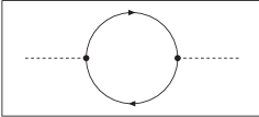
Figure 1: Bosonic mass correction due to fermion fluctuations. Fermionic lines are solid with an arrow, bosonic or ”mean field lines” $\sim\langle\bar{\psi}\left(\frac{1-\gamma^{5}}{2}\right)\psi\rangle$ are dashed.

$$\Gamma^{(\textrm{F})}_{1}=-4v_{4}\int^{\Lambda^{2}}_{0}dx\,x\ln(x+h^{2}_{\sigma}\phi^{\star}\phi).$$ (10)

From this one finds the mean field effective action

$$\Gamma^{(\textrm{F})} = \Gamma^{(\textrm{F})}_{0}+\Gamma^{(\textrm{F})}_{1}$$

$$= \left(\mu^{2}_{\sigma}-4v_{4}h^{2}_{\sigma}\Lambda^{2}\right)\phi^{\star}\phi+\textrm{const}+{\mathcal{O}}\left((\phi^{\star}\phi)^{2}\right),$$

where we have expanded in powers of $\phi$. The mass term turns negative if

$$\frac{2\mu^{2}_{\sigma}}{h^{2}_{\sigma}\Lambda^{2}}<8v_{4},$$ (12)

As it should be this result only depends on the ratio $h^{2}_{\sigma}/\mu^{2}_{\sigma}=2\lambda_{\sigma}$.

We now want to determine the critical line in the plane of invariant couplings $\bar{\lambda}_{\sigma}$, $\bar{\lambda}_{V}$ from the condition (12), i.e.

$$\lambda^{\textrm{crit}}_{\sigma}=\frac{1}{8v_{4}\Lambda^{2}}.$$ (13)

Using the relation (3) we infer a linear dependence of $\bar{\lambda}^{\textrm{crit}}_{\sigma}$ on $\gamma$ whenever $\bar{\lambda}_{V}\neq 0$

$$\bar{\lambda}^{\textrm{crit}}_{\sigma}=\frac{1}{8v_{4}\Lambda^{2}}-2\gamma\bar{\lambda}_{V}.$$ (14)

(For numerical values see Tabs. 1 and 13). This dependence is a major shortcoming of MFT. We will refer to it as the ”Fierz ambiguity”. The Fierz ambiguity does not only affect the critical couplings but also influences the values of masses, effective couplings etc..

The origin of the Fierz ambiguity can be traced back to the treatment of fluctuations. A FT of the type (2) changes the effective mean field. In a symbolic language a FT maps $(\bar{\psi}_{a}\psi_{a})(\bar{\psi}_{b}\psi_{b})\rightarrow(\bar{\psi}_{a}\psi_{b})(\bar{\psi}_{b}\psi_{a})$ where the brackets denote contraction over spinor indices and matrices $\sim\gamma_{\mu}$ or $\sim\gamma^{5}$ are omitted. A mean field $\bar{\psi}_{a}\psi_{a}$, appears after the FT as $\bar{\psi}_{a}\psi_{b}$. From the viewpoint of the fluctuations one integrates out different fluctuating fields before and after the FT. It is therefore no surprise that all results depend on $\gamma$.

III Partial Bosonization

The MFT calculation introduces ”mean fields” composed of fermion - antifermion (or fermion - fermion) bilinears. This is motivated by the fact that in many physical systems the fermions are not the only relevant degrees of freedom at low energies. Bosonic bound states become important and may condense. Examples are Cooper pairs in superconductivity or mesons in QCD. For a detailed description of the interplay between fermionic and composite bosonic fluctuations it seems appropriate to treat both on equal footing by introducing explicit fields for the relevant composite bosons. This will also shed more light on the status of MFT.

Partial bosonization Ellwanger:1994wy ; Berges:1999eu ; stratonovich ; Hubbard:1959ub is achieved by introducing unit factors in the functional integral for the partition function

$$Z = \int{\mathcal{D}}\bar{\psi}{\mathcal{D}}\psi\exp\left(-\textrm{S}[\psi]\right)$$

$$= \int{\mathcal{D}}\bar{\psi}{\mathcal{D}}\psi{\mathcal{D}}\phi{\mathcal{D}}V^{\mu}{\mathcal{D}}A^{\mu}{\mathcal{N}}_{\phi}{\mathcal{N}}_{V}{\mathcal{N}}_{A}\exp\left(-\textrm{S}[\psi]\right)$$

with

$${\mathcal{N}}_{\phi} = \exp\bigg{[}-\mu^{2}_{\sigma} \left(\phi^{\star}+\frac{h_{\sigma}}{2\mu^{2}_{\sigma}}\bar{\psi}(1+\gamma^{5})\psi\right)$$ (16)

$$\times\left(\phi-\frac{h_{\sigma}}{2\mu^{2}_{\sigma}}\bar{\psi}(1-\gamma^{5})\psi\right)\bigg{]},$$

$${\mathcal{N}}_{V} = \,\exp\bigg{[}-\frac{\mu^{2}_{V}}{2} \left(V^{\mu}-\frac{h_{V}}{\mu^{2}_{V}}\bar{\psi}\gamma^{\mu}\psi\right)$$

$$\times\left(V_{\mu}-\frac{h_{V}}{\mu^{2}_{V}}\bar{\psi}\gamma_{\mu}\psi\right)\bigg{]},$$

$${\mathcal{N}}_{A} = \,\exp\bigg{[}-\frac{\mu^{2}_{A}}{2} \left(A^{\mu}-\frac{h_{A}}{\mu^{2}_{A}}\bar{\psi}\gamma^{\mu}\gamma^{5}\psi\right)$$

$$\times\left(A_{\mu}-\frac{h_{A}}{\mu^{2}_{A}}\bar{\psi}\gamma_{\mu}\gamma^{5}\psi\right)\bigg{]}.$$

The action in the ”bosonic language” is composed of the original fermionic action and the arguments of the exponentials in ${\mathcal{N}}_{\phi}$, ${\mathcal{N}}_{V}$ and ${\mathcal{N}}_{A}$. Using the relation (5) one finds that the quartic fermion interaction is cancelled. It is now replaced by mass terms for the bosons and Yukawa couplings between bosons and fermions as given by the expression (4).

Since the action, Eq. (4), is quadratic in the fermionic fields the functional integral over the fermionic degrees of freedom is Gaussian and can be done in one step. As we have seen in the previous section this precisely leads to the MFT results. More precisely, we understand now that for different choices of $\gamma$ the MFT treatment leaves out different bosonic fluctuations. In this context we note that the bosonic potential in the bosonized effective action must be bounded from below. This restricts the possible couplings to $\lambda_{\sigma},\lambda_{V},\lambda_{A}>0$. In the invariant variables this restriction translates to $\bar{\lambda}_{\sigma},\bar{\lambda}_{V}>0$ and for $\gamma$ it implies $0<\gamma<1$.

IV Perturbation Theory

In order to cure the unpleasant dependence of the MFT result on $\gamma$ we will include part of the bosonic fluctuations in sects. VI and VII. Some guidance for the level of approximations needed can be gained from perturbation theory in the fermionic language. Since the four fermion vertex is uniquely characterized by $\bar{\lambda}_{\sigma}$ and $\bar{\lambda}_{V}$ the perturbative result must be independent of $\gamma$ at any given loop order. The lowest order corrections to the four fermion couplings are obtained by expanding the one-loop expression

$$\Delta\Gamma^{\textrm{(1-loop)}}=\frac{1}{2}STr\left[\ln\left(\textrm{S}^{(2)}\right)\right]=-Tr\left[\ln\left(\textrm{S}^{(2)}_{\bar{F}F}\right)\right]$$ (17)

up to order $(\bar{\psi}\psi)^{2}$. The corresponding graphs are shown in the second panel of Fig. 4. From

$$\Delta \Gamma^{\textrm{(1-loop)}}=v_{4}\Lambda^{2}\bigg{\{}$$ (18)

$$[4\lambda^{2}_{\sigma}-4\lambda_{\sigma}(\lambda_{A}-2\lambda_{V})]\left[\left(\bar{\psi}\psi\right)^{2}-\left(\bar{\psi}\gamma^{5}\psi\right)^{2}\right]$$

$$+[-2\lambda_{\sigma}\lambda_{V}+4(\lambda_{A}-\lambda_{V})\lambda_{V}]\left[\left(\bar{\psi}\gamma^{\mu}\psi\right)^{2}\right]$$

$$+\left[-\lambda^{2}_{\sigma}+2\lambda_{\sigma}\lambda_{A}+3\lambda^{2}_{V}-2\lambda_{A}\lambda_{V}-\lambda^{2}_{A}\right]\left[\left(\bar{\psi}\gamma^{\mu}\gamma^{5}\psi\right)^{2}\right]\bigg{\}}.$$

we can read off the corrections $\Delta\lambda_{\sigma}$, $\Delta\lambda_{V}$ and $\Delta\lambda_{A}$ to the coupling constants. In order to establish that our result is independent of $\gamma$ we use the freedom of FT to bring our results into a standard form, such that $\frac{\Delta\lambda_{A}}{\Delta\lambda_{V}}=\frac{\gamma}{1-\gamma}$. Inserting next the invariant variables (3) leads to:

$$\Delta\bar{\lambda}_{\sigma} = 4v_{4}\Lambda^{2}(\bar{\lambda}^{2}_{\sigma}+4\bar{\lambda}_{\sigma}\bar{\lambda}_{V}+3\bar{\lambda}^{2}_{V}),$$ (19)

$$\Delta\bar{\lambda}_{V} = 2v_{4}\Lambda^{2}(\bar{\lambda}_{\sigma}+\bar{\lambda}_{V})^{2}.$$

In contrast to MFT the result does not depend on $\gamma$.

The perturbative result, Eq. (19), always leads to finite corrections to the coupling constants. Remembering that in the fermionic language the onset of SSB is marked by a divergence of the coupling constants, it becomes clear that we will never get SSB in perturbation theory. No critical couplings can be calculated. This is a severe shortcoming of perturbation theory which cannot be overcome by calculating higher loop orders. Only an infinite number of loops can give SSB. In the next section we establish how a renormalization group treatment can overcome this difficulty without encountering the Fierz ambiguity of MFT. A calculation of the critical coupling becomes feasible. Nevertheless, even this RG-treatment has its limitations once the couplings diverge. In particular, it does not allow us to penetrate the phase with SSB. In sects. VI and VII this shortcoming will be cured by a RG-treatment in the partially bosonized language. In particular, we will see in sect. VII which diagrams are needed in order to maintain the independence of results on $\gamma$ in analogy to perturbation theory.

V Renormalization Group for Fermionic Interactions

The renormalization group equations for the effective average action Wetterich:1993be are obtained by adding a $k$-dependent infrared cutoff term $\Delta S_{k}$ to the action. The effective average action $\Gamma_{k}$ results from a Legendre transform of $\ln Z_{k}$ Wetterich:1993be . Due to the infrared cutoff, $\Gamma_{k}$ receives only contributions from fluctuations with $q^{2}\gtrsim k^{2}$. We take $\Delta\textrm{S}_{k}$ quadratic in the fermion fields,

$$\Delta\textrm{S}_{k}=\int\frac{d^{4}q}{(2\pi)^{4}}\bar{\psi}(q)R_{k}(q)\psi(q)$$ (20)

with $R_{k}$ vanishing fast for $q^{2}\gg k^{2}$. For a cutoff function which diverges for $k\rightarrow\infty$ and vanishes for $k\rightarrow 0$ the functional $\Gamma_{k}$ interpolates between the ”classical action” $\Gamma_{\infty}=\textrm{S}_{\textrm{F}}$ and the full effective action $\Gamma_{0}=\Gamma$ which includes all quantum fluctuations. The $k$-dependence of $\Gamma_{k}$ is governed by the following exact equation ($t=\ln(k)$):

$$\partial_{t}\Gamma_{k}[\psi] = \frac{1}{2}STr\left\{\tilde{\partial}_{t}\ln(\Gamma^{(2)}_{k}[\psi]+R_{k})\right\},$$ (21)

$$\tilde{\partial}_{t} = \partial_{t}R_{k}\frac{\partial}{\partial R_{k}}.$$

with $\Gamma^{(2)}_{k}$ the second functional derivative of $\Gamma_{k}$ with respect to the fermion fields. Despite its suggestive one-loop form this is a functional differential equation which cannot be solved exactly.

A first approximation neglects the $k$-dependence of $\Gamma_{k}$ on the right hand side (RHS). The solution is the perturbative result, Eq. (17). As we have seen in the previous sect. IV this approximation does not lead to SSB. For a better approximation we restrict $\Gamma_{k}$ to the terms specified in Eq. (I) but take all couplings explicitly $k$-dependent. In the action (I) we have only local interactions. Expressed in momentum space the four fermion interactions have no momentum dependence. This is often referred to as the local potential approximation (LPA) Tetradis:1993ts ; Hasenfratz:1986dm ; Morris:1994ki .

Decomposing the fluctuation matrix $\Gamma^{(2)}_{k}$ according to

$$\Gamma^{(2)}_{k}+R_{k}={\mathcal{P}}+{\mathcal{F}}$$ (22)

into a field independent part ${\mathcal{P}}$ (inverse propagator) and a field dependent part ${\mathcal{F}}$ we can expand the RHS of Eq. (21) as follows:

$$\partial_{t}\Gamma_{k} = \frac{1}{2}STr\{\tilde{\partial}_{t}\left(\frac{1}{\mathcal{P}}\mathcal{F}\right)\}-\frac{1}{4}STr\{\tilde{\partial}_{t}\left(\frac{1}{\mathcal{P}}\mathcal{F}\right)^{2}\}$$

$$+ \frac{1}{6}STr\{\tilde{\partial}_{t}\left(\frac{1}{\mathcal{P}}\mathcal{F}\right)^{3}\}-\frac{1}{8}STr\{\tilde{\partial}_{t}\left(\frac{1}{\mathcal{P}}\mathcal{F}\right)^{4}\}+\cdots.$$

This amounts to an expansion in powers of fields and we can compare the coefficients of the four fermion terms with the couplings specified by Eq. (I). We obtain a set of ordinary differential equations for the couplings:

$$\partial_{t}\bar{\lambda}_{\sigma,k} = -8v_{4}l^{(F),4}_{1}(s)k^{2}(\bar{\lambda}^{2}_{\sigma,k}+4\bar{\lambda}_{\sigma,k}\bar{\lambda}_{V,k}+3\bar{\lambda}^{2}_{V,k}),$$

$$\partial_{t}\bar{\lambda}_{V,k} = -4v_{4}l^{(F),4}_{1}(s)k^{2}(\bar{\lambda}_{\sigma,k}+\bar{\lambda}_{V,k})^{2},$$ (24)

in agreement with Aoki:1997fh where the same model has been studied. The threshold functions $l^{(F),4}_{1}$ are defined in Berges:2000ew . For our actual calculation we use a linear cutoff Litim:2000ci and adapt the threshold functions to our setting with fixed momentum cutoff $q^{2}<\Lambda^{2}$ in App. A. The dependence on $s=k^{2}/\Lambda^{2}$ becomes relevant only for $k>\Lambda$ whereas for $k<\Lambda$ one has constants $l^{(F),4}_{1}=1/2$.

The fermionic flow equations (V) do not depend on $\gamma$. In a diagrammatic language we again have evaluated the diagrams of Fig. 4 (second panel) but now with $k$-dependent vertices. In the RG-formulation we only go a tiny step $\Delta k$, and reinsert the resulting couplings (one-loop diagrams) before we go the next step. This leads to a resummation of loops. Since Eq. (V) is now nonlinear (quadratic terms on the RHS) the couplings can and do diverge for a finite $k$ if the initial couplings are large enough. Therefore we observe the onset of SSB and find a critical coupling. Since Eq. (V) is invariant this critical coupling does not depend on $\gamma$! Values for the critical coupling obtained by numerically solving Eq. (V) can be found in Tabs. 1 and 13.

The next step in improving this calculation in the fermionic language would be to take the momentum dependence of the couplings into account (e.g. Meggiolaro:2001kp ) or to include higher orders of the fermionic fields into the truncation. This seems quite complicated and at first sight we have no physical guess what is relevant. The renormalization group treatment of the bosonic formulation in sect. III seems much more promising in this respect.

VI Bosonic flow

The flow equations in the bosonic language are obtained in complete analogy with the fermionic formulation. In this paper we restrict the discussion to a ”pointlike” truncation as given by Eq. (4) with $k$-dependent couplings. We will see that in this approximation we reproduce the result of the last section if we take care of the fact that new fermionic interactions are generated by the flow and have to be absorbed by an appropriate $k$-dependent redefinition of the bosonic fields. The crucial advantage of the bosonic formulation is that it can easily be extended. For example, the bosonic bound states become dynamical fields if we allow for appropriate kinetic terms in the truncation, i.e.

$$\Delta\Gamma_{\textrm{kin}}\!\!\! = \!\!\!\!\int\!d^{4}x\bigg{\{}Z_{\phi}\partial_{\mu}\phi^{\star}\partial^{\mu}\phi+\frac{Z_{V}}{4}V_{\mu\nu}V^{\mu\nu}+\frac{Z_{A}}{4}A_{\mu\nu}A^{\mu\nu}$$ (25)

$$\quad\quad\quad+\frac{Z_{V}}{2\alpha_{V}}(\partial_{\mu}V^{\mu})^{2}+\frac{Z_{A}}{2\alpha_{A}}(\partial_{\mu}A^{\mu})^{2}\bigg{\}}$$

with

$$V_{\mu\nu}=\partial_{\mu}V_{\nu}-\partial_{\nu}V_{\mu},\quad A_{\mu\nu}=\partial_{\mu}A_{\nu}-\partial_{\nu}A_{\mu}.$$ (26)

Also spontaneous symmetry breaking can be explicitly studied if we replace $\mu^{2}_{\sigma}\phi^{\star}\phi$ by an effective potential $U(\phi^{\star}\phi)$ which may have a minimum for $\phi\neq 0$. This approach has been followed in previous studies Schaefer:em ; Kodama:1999if ; Jungnickel:1995fp ; Bergerhoff:1999hr . In the present paper we will briefly pursue only the extension (25) since our main focus is the issue of the Fierz ambiguity.

It is instructive to neglect in a first step all bosonic fluctuations by putting all bosonic entries in the propagator matrix ${\mathcal{P}}^{-1}$ equal to zero. This removes all diagrams with internal bosonic lines. Among other things this neglects the vertex correction, Fig. 2, and therefore the running of the Yukawa couplings.

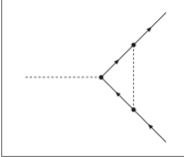
Figure 2: Vertex correction diagram in the bosonized model. Solid lines are fermions, dashed lines are bosons. There exist several diagrams of this type since we have different species of bosons.

Indeed, Fig. 1 is the only diagram contributing and we recover MFT. One obtains the flow equations

$$\partial_{t}\mu^{2}_{\sigma,k} = 8h^{2}_{\sigma,k}v_{4}k^{2}l^{(F),4}_{1}(s),$$

$$\partial_{t}\mu^{2}_{V,k} = 8h^{2}_{V,k}v_{4}k^{2}l^{(F),4}_{1}(s),$$

$$\partial_{t}\mu^{2}_{A,k} = 8h^{2}_{A,k}v_{4}k^{2}l^{(F),4}_{1}(s),$$

$$\partial_{t}h_{\sigma,k} = 0,\quad\partial_{t}h_{V,k}=0,\quad\partial_{t}h_{A,k}=0.$$ (27)

As long as we do not consider the wave function renormalization (25) for the bosons, the flow can be completely described in terms of the dimensionless combinations

$$\tilde{\epsilon}_{\sigma,k}=\frac{\mu^{2}_{\sigma,k}}{h^{2}_{\sigma,k}k^{2}},\quad\tilde{\epsilon}_{V,k}=\frac{\mu^{2}_{V,k}}{h^{2}_{V,k}k^{2}},\quad\tilde{\epsilon}_{A,k}=\frac{\mu^{2}_{A,k}}{h^{2}_{A,k}k^{2}}.$$ (28)

Due to the constant Yukawa couplings we can integrate Eq. (VI). We find critical couplings:

$$\frac{\mu^{2}_{\sigma}}{h^{2}_{\sigma}\Lambda^{2}}\mid_{\textrm{crit}}=4v_{4},\quad\frac{\mu^{2}_{V}}{h^{2}_{V}\Lambda^{2}}\mid_{\textrm{crit}}=4v_{4},\quad\frac{\mu^{2}_{A}}{h^{2}_{A}\Lambda^{2}}\mid_{\textrm{crit}}=4v_{4}.$$ (29)

These are, of course, the results of MFT, Eq. (12). We note that in Eq. (VI) the equations for the different species of bosons are completely decoupled. The mass terms do not turn negative at the same scale for the different species. Indeed it is possible that the mass of one boson species turns negative while the others do not. Such a behavior is expected for the full theory, whereas for the fermionic RG of sect. V all couplings diverge simultaneously due to their mutual coupling. However, no real conclusion can be taken from Eq. (29) because of the strong dependence on $\gamma$.

Now, let us take also the bosonic fluctuations into account. This includes the vertex correction, Fig. 2, and the flow of the Yukawa couplings does not vanish anymore. In the pointlike approximation $(Z_{\phi}=Z_{A}=Z_{V}=0)$ one obtains

$$\partial_{t}h^{2}_{\sigma,k}= - 32v_{4}l^{(F),4}_{1}(s)k^{2}h^{2}_{\sigma,k}\left[\frac{h^{2}_{V,k}}{\mu^{2}_{V,k}}-\frac{h^{2}_{A,k}}{\mu^{2}_{A,k}}\right],$$

$$\partial_{t}h^{2}_{V,k}= - 4v_{4}l^{(F),4}_{1}(s)k^{2}h^{2}_{V,k}$$

$$\times\left[\frac{h^{2}_{\sigma,k}}{\mu^{2}_{\sigma,k}}+2\left(\frac{h^{2}_{V,k}}{\mu^{2}_{V,k}}+\frac{h^{2}_{A,k}}{\mu^{2}_{A,k}}\right)\right],$$

$$\partial_{t}h^{2}_{A,k}= - 4v_{4}l^{(F),4}_{1}(s)k^{2}h^{2}_{A,k}$$ (30)

$$\times\left[-\frac{h^{2}_{\sigma,k}}{\mu^{2}_{\sigma,k}}+2\left(\frac{h^{2}_{V,k}}{\mu^{2}_{V,k}}+\frac{h^{2}_{A,k}}{\mu^{2}_{A,k}}\right)\right].$$

Using the dimensionless $\tilde{\epsilon}$’s we now find:

$$\partial_{t}\tilde{\epsilon}_{\sigma,k} = -2\tilde{\epsilon}_{\sigma,k}+8\left[1+4\left(\frac{\tilde{\epsilon}_{\sigma,k}}{\tilde{\epsilon}_{V,k}}-\frac{\tilde{\epsilon}_{\sigma,k}}{\tilde{\epsilon}_{A,k}}\right)\right]v_{4}l^{(F),4}_{1}(s),$$

$$\partial_{t}\tilde{\epsilon}_{V,k} = -2\tilde{\epsilon}_{V,k}+8\left[2+\left(\frac{\tilde{\epsilon}_{V,k}}{2\tilde{\epsilon}_{\sigma,k}}+\frac{\tilde{\epsilon}_{V,k}}{\tilde{\epsilon}_{A,k}}\right)\right]v_{4}l^{(F),4}_{1}(s),$$

$$\partial_{t}\tilde{\epsilon}_{A,k} = -2\tilde{\epsilon}_{A,k}+8\left[2-\left(\frac{\tilde{\epsilon}_{A,k}}{2\tilde{\epsilon}_{\sigma,k}}-\frac{\tilde{\epsilon}_{A,k}}{\tilde{\epsilon}_{V,k}}\right)\right]v_{4}l^{(F),4}_{1}(s).$$

The onset of spontaneous symmetry breaking is indicated by a vanishing of $\tilde{\epsilon}$ for at least one species of bosons. Large $\tilde{\epsilon}$ means that the corresponding bosonic species becomes very massive and therefore effectively drops out of the flow.

For initial couplings larger than the critical values (see Tabs. 1 and 13) both $\tilde{\epsilon}_{\sigma,k}$ and $\tilde{\epsilon}_{V,k}$ reach zero for finite $t$. Due to the coupling between the different channels they reach zero at the same $t$. At this point $\tilde{\epsilon}_{A,k}$ reaches infinity and drops out of the flow. This is quite different from the flow without the bosonic fluctuations where the flow equations for the different species were decoupled. The breakdown of all equations at one point resembles now the case of the fermionic model discussed in sect. V. The $\gamma$-dependence of the critical couplings is reduced considerably, as compared to MFT. This shows that the inclusion of the bosonic fluctuations is crucial for any quantitatively reliable result. Nevertheless, the difference between the bosonic and the fermionic flow remains of the order of $10\%$.

VII Adapted Bosonic Flow

In our truncation the bosonic propagators are approximated by constants $\mu^{-2}_{k}$. The exchange of bosons therefore produces effective pointlike four fermion interactions. One therefore would suspect that this approximation should contain the same information as the fermionic formulation with pointlike four fermion interactions. An inspection of the results in Tabs. 1, 13 shows, however, that this is not the case for the formulation of the preceding section. In particular, in contrast to the fermionic language the results of the bosonic flow equations still depend on the unphysical parameter $\gamma$.

In fact, even for small couplings $\lambda$ the bosonic flow equations of sect. VI do not reproduce the perturbative result. The reason is that at the one-loop level new quartic fermion interactions are generated by the box diagrams shown in Fig. 3. An easy inspection shows that they contribute in the same order $\lambda^{2}$ as the diagrams in Figs. 1 and 2. Even if we start from vanishing quartic couplings after partial bosonization, such couplings are generated by the flow. The diagrams in Fig. 3 yield

$$\partial_{t}\lambda_{\sigma,k} = \beta_{\lambda_{\sigma}}=-8v_{4}l^{(F),4}_{1}(s)k^{2}\frac{h^{2}_{\sigma,k}}{\mu^{2}_{\sigma,k}}\frac{h^{2}_{A,k}}{\mu^{2}_{A,k}}+4k^{-2}\tilde{\gamma}(k),$$

$$\partial_{t}\lambda_{V,k} = \beta_{\lambda_{V}}=24v_{4}l^{(F),4}_{1}(s)k^{2}\frac{h^{2}_{V,k}}{\mu^{2}_{V,k}}\frac{h^{2}_{A,k}}{\mu^{2}_{A,k}}-2k^{-2}\tilde{\gamma}(k),$$

$$\partial_{t}\lambda_{A,k} = \beta_{\lambda_{A}}=-v_{4}l^{(F),4}_{1}(s)k^{2}$$

$$\times\left[\frac{h^{4}_{\sigma,k}}{\mu^{4}_{\sigma,k}}-12\frac{h^{4}_{V,k}}{\mu^{4}_{V,k}}-12\frac{h^{4}_{A,k}}{\mu^{4}_{A,k}}\right]+2k^{-2}\tilde{\gamma}(k).$$

Here $\tilde{\gamma}(k)$ is an in principle arbitrary function of scale determining the choice of FT for the generated four fermion interactions. We will make a special choice of this function (similar to the one made in sects. IV and V) namely we require

$$\frac{\tilde{\epsilon}_{V,k}}{\tilde{\epsilon}_{A,k}}=\frac{\gamma}{1-\gamma}\quad\forall\,k,$$ (33)

with $\tilde{\epsilon}$ given in Eq. (28). The resulting equation $\partial_{t}(\tilde{\epsilon}_{V,k}/\tilde{\epsilon}_{A,k})=0$ fixes $\tilde{\gamma}(k)$. An improved choice of $\tilde{\gamma}(k)$ can be obtained once the momentum dependence of vertices is considered more carefully Gies:2002nw .

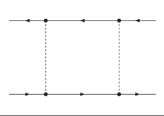
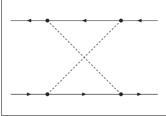
Figure 3: Box diagrams for the bosonized model. Again, solid lines are fermions, dashed lines bosons and vertices are marked with a dot. The diagrams generate new four fermion interactions even for the model (4) without direct four fermion interactions.

An inclusion of the couplings $\lambda_{k}$ into the truncation of the effective average action does not seem very attractive. Despite the partial bosonization we would still have to deal with the multi-fermion interactions and the bosonic formulation would be of even higher algebraic complexity than the fermionic formulation. A way out of this has been proposed in Gies:2002nw . There, it has been shown that it is possible to reabsorb all four fermion interactions generated during the flow by a redefinition of the bosonic fields. In the following brief description of this method we use a very symbolic notation.

Introducing an explicit $k$-dependence for the definition of the bosonic fields in terms of fermion bilinears, the flow equation Eq. (21) is modified:

$$\partial_{t}\Gamma_{k}=\partial_{t}\Gamma_{k}\mid_{\phi_{k}}+\frac{\delta\Gamma_{k}}{\delta\phi_{k}}\partial_{t}\phi_{k}.$$ (34)

Here $\partial_{t}\Gamma_{k}\mid_{\phi_{k}}=\partial_{t}\Gamma_{k}\mid$ is the standard flow of the effective average action at fixed fields. Shifting $\phi$ by

$$\partial_{t}\phi_{k}=\left(\bar{\psi}\psi\right)\partial_{t}\omega_{k}$$ (35)

we find

$$\partial_{t}\mu^{2}=\partial_{t}\mu^{2}\mid,$$ (36)

$$\partial_{t}h=\partial_{t}h\mid+\mu^{2}\partial_{t}\omega_{k},\quad\partial_{t}\lambda=\partial_{t}\lambda\mid-h\partial_{t}\omega_{k}$$

and we can choose $\omega_{k}$ to establish:

$$\partial_{t}\lambda=0.$$ (37)

Instead of including running four fermion couplings explicitly we therefore only have to use adapted flow equations for the couplings contained in Eq. (4).

Let us now apply this method explicitly to our model. Shifting

$$\partial_{t}\phi=-\bar{\psi}\left(\frac{1-\gamma^{5}}{2}\right)\psi\partial_{t}\omega_{\sigma,k},$$ (38)

$$\partial_{t}\phi^{\star}=\bar{\psi}\left(\frac{1+\gamma^{5}}{2}\right)\psi\partial_{t}\omega_{\sigma,k},$$

$$\partial_{t}V^{\mu}=-\bar{\psi}\gamma^{\mu}\psi\partial_{t}\omega_{V,k},\quad\partial_{t}A^{\mu}=-\bar{\psi}\gamma^{\mu}\gamma^{5}\psi\partial_{t}\omega_{A,k}$$

we have

$$\partial_{t}\lambda_{\sigma,k} = \partial_{t}\lambda_{\sigma,k}|-h_{\sigma,k}\partial_{t}\omega_{\sigma,k},$$ (39)

$$\partial_{t}\lambda_{V,k} = \partial_{t}\lambda_{V,k}|-2h_{V,k}\partial_{t}\omega_{V,k},$$

$$\partial_{t}\lambda_{A,k} = \partial_{t}\lambda_{A,k}|-2h_{A,k}\partial_{t}\omega_{A,k}.$$

Requiring $\partial_{t}\lambda=0$ for all $\lambda$’s we can determine the functions $\omega$:

$$\partial_{t}\omega_{\sigma,k}=\frac{\beta_{\lambda_{\sigma}}}{h_{\sigma,k}},\quad\partial_{t}\omega_{V,k}=\frac{\beta_{\lambda_{V}}}{2h_{V,k}},\quad\partial_{t}\omega_{A,k}=\frac{\beta_{\lambda_{A}}}{2h_{A,k}}$$ (40)

with the $\beta$-functions given in Eq. (VII). This yields the adapted flow equations for the Yukawa couplings

$$\partial_{t}h_{\sigma,k} = \partial_{t}h_{\sigma,k}|+\mu^{2}_{\sigma,k}\partial_{t}\omega_{\sigma,k},$$ (41)

$$\partial_{t}h_{V,k} = \partial_{t}h_{V,k}|+\mu^{2}_{V,k}\partial_{t}\omega_{V,k},$$

$$\partial_{t}h_{A,k} = \partial_{t}h_{A,k}|+\mu^{2}_{A,k}\partial_{t}\omega_{A,k}.$$

Combining Eqs. (VI), (VII), (33), (40), (41) determines $\tilde{\gamma}(k)$

$$\tilde{\gamma}(k) = 2v_{4}l^{(F),4}_{1}(s)$$

$$\times \left[-\frac{3}{\tilde{\epsilon}^{2}_{V,k}}+\frac{1}{\tilde{\epsilon}_{V,k}\tilde{\epsilon}_{A,k}}+\frac{(4\tilde{\epsilon}_{\sigma,k}-\tilde{\epsilon}_{A,k})^{2}}{4\tilde{\epsilon}^{2}_{\sigma,k}\tilde{\epsilon}_{A,k}(\tilde{\epsilon}_{V,k}+\tilde{\epsilon}_{A,k})}\right].$$

Having fixed the ratio between $\tilde{\epsilon}_{V,k}$ and $\tilde{\epsilon}_{A,k}$ we need only two equations to describe the flow. We will use the ones for $\tilde{\epsilon}_{\sigma,k}$ and $\bar{\epsilon}_{V,k}=(1-\gamma)\tilde{\epsilon}_{V,k}$

$$\partial_{t}\tilde{\epsilon}_{\sigma,k}=-2\tilde{\epsilon}_{\sigma,k} + 4[(1+\gamma)-4(-2+\gamma+2\gamma^{2})\frac{\tilde{\epsilon}_{\sigma,k}}{\bar{\epsilon}_{V,k}}$$

$$+ 4(3-7\gamma+4\gamma^{3})\frac{\tilde{\epsilon}^{2}_{\sigma,k}}{\bar{\epsilon}^{2}_{V,k}}]l^{(F),4}_{1}(s)v_{4},$$

$$\partial_{t}\bar{\epsilon}_{V,k}=-2\bar{\epsilon}_{V,k} + 4[\frac{\bar{\epsilon}_{V,k}}{2\tilde{\epsilon}_{\sigma,k}}-(2\gamma-1)]^{2}l^{(F),4}_{1}(s)v_{4}.$$

These equations are completely equivalent to the fermionic flow Eq. (V). In order to see this we remember that the simple truncation of the form (4) is at most quadratic in the bosonic fields. We can therefore easily solve the bosonic field equations as a functional of the fermion fields. Reinserting the solution into the effective average action we obtain the form (I) with the $k$-dependent quartic couplings

$$\bar{\lambda}_{\sigma,k}=\frac{1}{2k^{2}\tilde{\epsilon}_{\sigma,k}}-2\gamma\frac{1}{k^{2}\bar{\epsilon}_{V,k}},\quad\bar{\lambda}_{V,k}=\frac{1}{k^{2}\bar{\epsilon}_{V,k}}.$$ (44)

Inserting this into Eq. (VII) we find Eq. (V), establishing both the exact equivalence to the fermionic model and the $\gamma$-independence of physical quantities.

On this level of truncation the equivalence between the fermionic and the adapted bosonic flow can also be seen on a diagrammatic level. As long as we do not have a kinetic term for the bosons the internal bosonic lines shrink to points. On the one-loop level we find an exact correspondence between the diagrams for the bosonized and the purely fermionic model summarized in Fig. 4. This demonstrates again that one-loop accuracy cannot be obtained without adaptation of the flow.

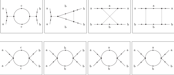
Figure 4: Summary of all diagrams encountered in the previous sections. There is a one to one correspondence between the diagrams of the bosonized model (first row) and the purely fermionic model (second row). Solid lines with an arrow denote fermionic lines. The letters in the diagrams are given to visualize the ways in which the fermionic operators are contracted, e.g. the first diagram in the second row results from a term $[(\bar{\psi}_{a}\psi_{a})(\bar{\psi}_{c}\psi_{c})][(\bar{\psi}_{c}\psi_{c})(\bar{\psi}_{b}\psi_{b})]$. Shrinking bosonic lines (dashed) to points maps the diagrams in the first row to the second row. In the approximations of sect. VI only the first or the first two diagrams are taken into account.

VIII The Schwinger-Dyson Approach

Finally, we compare in this section the results of MFT and the RG-treatment with the Schwinger-Dyson (SD) approach Schwinger:1951ex ; Dyson:1949ha . On the exact level the RG and SD approaches are equivalent in the sense that the propagator and higher N-point functions calculated using the flow equation (21) are also solutions of the SD-equations Ellwanger:1996wy ; Terao:2000ae . Nevertheless, once truncations are used the results will, in general, differ. The RG-equations resum diagrams beyond the leading order SD-equation.

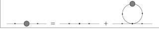
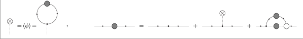
Figure 5: Diagrammatic representation of the lowest order Schwinger-Dyson equations for the fermionic model (a) (Eq. (I)) and the partially bosonized model (b) (Eq. (4)). The shaded circles depict the full propagator, the circle with the cross is the expectation value of the bosonic field and the empty circle is the full Yukawa vertex.

We start with the purely fermionic model (I). For this model the Schwinger-Dyson equation, approximated to lowest order, is depicted in Fig. 5. It is a closed equation since only the bare four fermion vertex appears. (Only higher order terms involve the full four fermion vertex.) We write the full fermionic propagator $G_{\textrm{F}}$ as

$$G^{-1}_{\textrm{F}}(p)=G^{-1}_{\textrm{F}0}(p)+\Sigma_{\textrm{F}}(p)$$ (45)

with the free propagator $G_{\textrm{F}0}$ and self-energy $\Sigma_{\textrm{F}}$. Using this one obtains a gap equation for the self-energy which can be solved self-consistently. To simplify the discussion we make an ansatz for the self-energy:

$$\Sigma_{\textrm{F}}=M_{\textrm{F}}\gamma^{5},$$ (46)

where the effective fermion mass $M_{\textrm{F}}$ obeys the gap equation

$$M_{\textrm{F}}=8v_{4}\left[\bar{\lambda}_{\sigma}+\bar{\lambda}_{V}\right]\int^{\Lambda^{2}}_{0}dx\,x\frac{M_{\textrm{F}}}{x+M^{2}_{\textrm{F}}}.$$ (47)

The onset for nontrivial solutions determines the critical couplings:

$$\left[\bar{\lambda}_{\sigma}+\bar{\lambda}_{V}\right]_{\textrm{crit}}=\frac{1}{8v_{4}\Lambda^{2}}.$$ (48)

This result is shown in Tabs. 1, 13 and does not depend on $\gamma$, as expected for a fermionic calculation. We observe that the MFT-result for the $\bar{\lambda}^{\textrm{crit}}_{\sigma}$ coincides with the SD-approach for a particular choice $\gamma=1/2$. However, in general MFT is not equivalent to the lowest order SD-equation. This can be seen by computing also the critical coupling for the onset of SSB in the vector channel. The MFT and SD results do not coincide for the choice $\gamma=1/2$.

Next, we turn to the SD-equations for the bosonized model (4) which are depicted in Fig. 5. We will make here two further approximations by replacing in the last graph of Fig. 5 the full fermion-fermion-boson vertex by the classical Yukawa coupling and the full bosonic propagator by $\mu^{-2}_{\textrm{B}}$. We remain with two coupled equations.

In a first step we approximate these equations even further by neglecting the last diagram in Fig. 5 altogether. Then no fermionic propagator appears on the right hand side of the equation for the fermionic propagator which only receives a mass correction for $\langle\phi\rangle\neq 0$. Without loss of generality we take $\phi$ real such that $M_{\textrm{F}}=h_{\sigma}\phi$ and

$$G^{-1}_{\textrm{F}}(q)=-q\!\!\!/+h_{\sigma}\phi\gamma^{5}.$$ (49)

Inserting this into the equation for the expectation value $\phi$ we find

$$\phi=\frac{4v_{4}}{\mu^{2}_{\sigma}}\int^{\Lambda^{2}}_{0}dx\,x\frac{h^{2}_{\sigma}\phi}{x+h^{2}_{\sigma}\phi^{2}}.$$ (50)

For the onset of nontrivial solutions we now find the critical value

$$\left[\frac{h^{2}_{\sigma}}{2\mu^{2}_{\sigma}}\right]_{\textrm{crit}}=\frac{1}{8v_{4}\Lambda^{2}}=\left[\bar{\lambda}_{\sigma}+2\gamma\bar{\lambda}_{V}\right]_{\textrm{crit}}$$ (51)

which is the (ambiguous) result from MFT given in Eqs. (12) and (14). This is not surprising since this exactly is MFT from the viewpoint of Schwinger-Dyson equations. Indeed, Eq. (50) is precisely the field equation which follows by differentiation of the MFT effective action (9) with respect to $\phi$,

$$\Gamma^{\textrm{(F)}}=\mu^{2}_{\sigma}\phi^{2}-4v_{4}\int^{\Lambda^{2}}_{0}dx\,x\ln(x+h^{2}_{\sigma}\phi^{2}).$$ (52)

In a next step we improve our approximation to include the full set of diagrams shown in Fig. 5. Using the same ansatz as before the self-energy $\Sigma_{\textrm{F}}$ now has two contributions,

$$\Sigma_{\textrm{F}}=M_{\textrm{F}}\gamma^{5}=h_{\sigma}\phi\gamma^{5}+\Delta m_{\textrm{F}}\gamma^{5}.$$ (53)

The first one is the contribution due to the expectation value of the bosonic field whereas $\Delta m_{\textrm{F}}$ is the contribution from the last diagram in Fig. 5, given by an integral which depends on $M_{\textrm{F}}$. Both in the equation for $\langle\phi\rangle$ and in the equation for the fermionic propagator only $M_{\textrm{F}}$ appears on the RHS. Inserting $\langle\phi\rangle$ in the graph, Fig. 5, one finds a gap equation which determines $M_{\textrm{F}}$:

$$M_{\textrm{F}}=8v_{4}\left[\frac{h^{2}_{\sigma}}{2\mu^{2}_{\sigma}}+\frac{h^{2}_{V}}{\mu^{2}_{V}}-\frac{h^{2}_{A}}{\mu^{2}_{A}}\right]\int^{\Lambda^{2}}_{0}dx\,x\frac{M_{\textrm{F}}}{x+M^{2}_{\textrm{F}}}.$$ (54)

Once more, this can be expressed in terms of the invariant couplings and again we arrive at Eq. (47).

Looking more closely at the two contributions to $M_{\textrm{F}}$ we find that alone neither the contribution $\sim\phi$ (which amounts to MFT as we have discussed above) nor the ”fermionic contribution” $\Delta m_{\textrm{F}}$ is invariant under FT’s. Only the combination $M_{\textrm{F}}$, which is the fermion mass and therefore a physical quantity, is invariant. Indeed, changing the FT amounts to a redefinition of the bosonic fields. In a very similar fashion to what we have done in sect. VII it allows us to choose bosonic fields such that $\Delta m_{\textrm{F}}=0$. Taking $\gamma=1/2$ gives us such a choice of the bosonic fields. This explains why MFT gives the same result as the purely fermionic calculation in this special case.

IX Beyond the pointlike approximation

In order to compare the size of the Fierz ambiguity with typical errors from the truncation we extend in this section our investigation beyond the pointlike approximation. We add to the general form of the effective action the bosonic propagator terms (25) with $\alpha_{V}=\alpha_{A}=1$. In order to simplify the numerical computations we choose in this section the ERGE-regularization scheme (cf. App. B) rather than a sharp ultraviolet momentum cutoff. As discussed in App. B the definition of the “classical couplings” $\bar{\lambda}_{\sigma}$, $\bar{\lambda}_{V}$ differs from the sharp cutoff regularization.

We have extended the truncation in consecutive steps in order to make the effect of various truncations directly visible. Our results are shown in Tab. 3. By comparing the first four rows of Tab. 3 with Tab. 13 we observe the effect of the different ultraviolet regularization. With the ERGE-definition of the “classical couplings” one finds a substantially larger value of the critical coupling $\bar{\lambda}^{\textrm{crit}}_{\sigma}$ than for the sharp cutoff regularization. This different size is purely a matter of definitions and not related to any approximation error. Let us now extend the truncation in the partially bosonized formulation step by step. As discussed above, the lowest order is MFT. As a typical size for the Fierz ambiguity we quote $\Delta_{\lambda}=\bar{\lambda}^{\textrm{crit}}_{\sigma}(\gamma=0.75)-\bar{\lambda}^{\textrm{crit}}_{\sigma}(\gamma=0.25)=-20$. The next step (1) includes the bosonic fluctuations in the pointlike approximation, without the adaption discussed in sect. VII. At this level the residual Fierz ambiguity is substantially reduced, $\Delta_{\lambda}=1.71$. Step (2) includes the adaption (box diagrams) in the pointlike approximation. Due to the equivalence with the pointlike approximation in the purely fermionic langauge there is no Fierz ambiguity at this level.

As a first step beyond the pointlike approximation we include the running of the wave function renormalizations (WFR) $Z_{\phi}$, $Z_{V}$, $Z_{A}$. (Details of the flow equations will be published elsewhere.) In step (3) this is done without the adaption by “rebosonization”. Omitting completely the rebosonization ((1)+(3)) yields $\Delta_{\lambda}=1.57$ whereas combining Eqs. (1), (2) and (3) results in $\Delta_{\lambda}=-0.31$. We finally use rebosonization also for the momentum dependence in the four fermion and Yukawa couplings generated by the flow (box diagrams and vertex corrections). The results depend somewhat on the detailed method (to be published elsewhere) and one finds $\Delta_{\lambda}=0.22$. It is impressive how the truncation reduces the Fierz ambiguity from a value $\Delta_{\lambda}=-20$ for MFT to a value $|\Delta_{\lambda}|<1$!

On the other hand, a comparison of the last rows in Tab. 3 yields a typical value for the remaining truncation error, $\bar{\lambda}^{\textrm{crit}}_{\sigma}=58\pm 5$. We emphasize that the quoted error should not be taken as an (more sophisticated) error estimate in a strict sense. A true error estimate is notoriously difficult in a situation without small parameters. One possibility would be further extensions of the truncation. One could also investigate the influence of different rebosonization procedures or the choice of different cutoff functions $R_{k}(q)$. Nevertheless, it seems convincing that we have reached a truncation uncertainty that is far less than the Fierz ambiguity in MFT (i.e. $|\Delta_{\lambda}|=20$). On the other hand, on this higher level of the truncation the residual Fierz ambiguity is already much less ($|\Delta_{\lambda}|<1$) than the truncation error. This is precisely what one would like to achieve for a successful non-perturbative approximation scheme in a partially bosonized setting.

In passing, we note that Schwinger-Dyson equations do a pretty good job in our context.

X Summary and Conclusions

We compare different approximation methods for a strongly interacting fermion system - the NJL model in our case. For this purpose we have computed the critical couplings for the onset of chiral symmetry breaking using mean field theory (MFT), fermionic and bosonic renormalization group methods (RG) and the Schwinger-Dyson equation (SD). This permits a direct comparison between the various methods. We believe that the general characteristics found here remain valid for other strongly interacting systems as well. For a sharp momentum cutoff the results for $\bar{\lambda}^{\textrm{crit}}_{\sigma}$ are summarized in Tabs. 1, 13 for two fixed values of $\bar{\lambda}_{V}$. Corresponding results for the ERGE regularization can be found in Tab. 3. Since the most characteristic features and problems of the different methods are most clearly seen when the couplings $\bar{\lambda}_{\sigma}$ and $\bar{\lambda}_{V}$ are of similar size we concentrate the discussion on Tab. 13.

All methods discussed here (except perturbation theory in sect. IV) correspond to non-perturbative resummations of perturbative diagrams. Both MFT and the lowest order SD sum only over fermionic fluctuations in presence of a bosonic background. They include, in principle, the same type of diagrams, Fig. 1. The MFT-result depends strongly on the choice of the background field. This ”Fierz ambiguity” is expressed by the dependence on the unphysical parameter $\gamma$ in the tables. No such ambiguity appears in the SD approach which therefore seems, at least at first sight, more reliable. We note that for a particular choice of $\gamma$ the MFT and the SD approaches give identical results - in our case $\gamma=1/2$. This has led to widespread belief that MFT and SD are equivalent if the basis for the Fierz ordering is appropriately chosen. However, this is not the case, as can be seen by calculating also the critical coupling where spontaneous symmetry breaking sets in in the vector channel (in the absence of other order parameters). There is again a value $\gamma=-(\bar{\lambda}_{\sigma}+\bar{\lambda}_{V})/(2\bar{\lambda}_{V})$ where MFT and SD give identical results, but it differs from $\gamma=1/2$ as encountered in the scalar channel. We conclude that there is no possible choice of $\gamma$ where both critical couplings for SSB in the scalar and vector channels are identical in the MFT and SD approaches. The conceptual and practical difference between the two approaches appears even more clearly if we consider a model with eight-fermion-couplings instead of a quartic coupling. Whereas in MFT the onset of SSB can be computed in one-loop order, only a three loop diagram contributes to the gap equation for $M_{\textrm{F}}$ in the SD approach. We also warn that the choice of $\gamma$ for which MFT and SD coincide in a given channel is not necessarily the optimal choice. Comparing the SD result (or the MFT result for $\gamma=1/2$), namely $\bar{\lambda}_{\sigma}=19.48$, with the perhaps more precise result from the renormalization group, $\bar{\lambda}_{\sigma}=14.62$, we see that an ”optimal choice” of the FT for the MFT approach may correspond to a value of $\gamma$ above $1/2$.

Approximation	Sect.	$\gamma=0$	0.25	0.5	0.75	1
MFT	II	39.48	38.48	37.48	36.48	35.48
Ferm. RG	V	41.54	41.54	41.54	41.54	41.54
Bos. RG	VI	36.83	36.88	36.95	37.02	37.12
Adapted Bos. RG	VII	41.54	41.54	41.54	41.54	41.54
SD	VIII	37.48	37.48	37.48	37.48	37.48

Table 1: Critical values $\bar{\lambda}^{\textrm{crit}}_{\sigma}$ for $\bar{\lambda}_{V}=2$ and for various values of the unphysical parameter $\gamma$ (with $\Lambda=1$). Progressing from MFT to the bosonic RG and adapted bosonic RG the dependence on $\gamma$ decreases as more and more diagrams are included. The Schwinger-Dyson result is independent of $\gamma$ but contains no vertex corrections in contrast to the RG-calculations.

Approximation	Sect.	$\gamma=0$	0.25	0.5	0.75	1
MFT	II	39.48	29.48	19.48	9.48	-0.52
Ferm. RG	V	14.62	14.62	14.62	14.62	14.62
Bos. RG	VI	15.44	13.39	13.45	15.55	19.46
Adapted Bos. RG	VII	14.62	14.62	14.62	14.62	14.62
SD	VIII	19.48	19.48	19.48	19.48	19.48

Table 2: The same as in Tab. 1 but with $\bar{\lambda}_{V}=20$.

Approximation	Chap.	$\gamma=0.1$	0.25	0.5	0.75	0.9
MFT	II	74.96	68.96	58.96	48.96	42.96
SD	VIII	58.96	58.96	58.96	58.96	58.96
Bos. RG=(1)	VI	53.16	52.93	53.32	54.64	55.88
Ad. Bos. RG=(1)+(2)	V	58.83	58.83	58.83	58.83	58.83
(1)+(3)	IX	53.90	53.66	54.00	55.23	56.37
(1)–(3)	IX	58.14	58.04	57.88	57.73	57.64
(1)–(4)	IX	61.60	61.69	61.82	61.91	61.94

Table 3: Critical coupling $\bar{\lambda}^{\textrm{crit}}_{\sigma}$ for $\bar{\lambda}_{V}=20$ for a UV regularization by the ERGE scheme We show different approximation steps: (1) the pointlike contibutions to the mass and the Yukawa coupling (Figs. 1, 2), (2) the pointlike contributions from the box diagrams (Fig. 3), (3) the contribution to the WFR from the purely bosonic diagram (Fig. 1) and (4) the contribution to the WFR from the momentum dependence of the diagrams 2 and 3 (those contribute again via an appropriate adaption of the flow).

Partial bosonization is a very powerful tool for understanding strongly interacting fermionic systems beyond the level of MFT or SD-equations. It allows us to treat the bosonic fluctuations in an explicit manner and provides for a rather simple framework for the discussion of SSB. Most importantly, it permits the direct exploration of the ordered phase which is, in practice, almost inaccessible for the fermionic RG. In order to permit a simple comparison with the fermionic RG we have used a very crude approximation for the purely bosonic sector by retaining only a mass term and neglecting bosonic interactions as well as the momentum dependence of the bosonic propagator. In this approximation the effect of the boson exchange between fermions does not go beyond pointlike fermionic interactions. Taking into account only the running of the Yukawa couplings (Fig. 2) in the bosonic RG of sect. VI, we observe already a very substantial decrease of the Fierz ambiguity as compared to MFT. The dependence on $\gamma$ is greatly reduced and the numerical value of the critical coupling comes already close to the result of the fermionic RG. These features can be compared to the inclusion of higher loop effects in perturbation theory in particle physics: they often reduce the dependence of the results on unphysical parameters, such as the choice of the renormalization scale.

As compared to perturbation theory, the box diagrams (3) are still missing in the discussion of sect. VI. This shortcoming is cured by the adapted bosonic renormalization group discussed in sect. VII. Here the relation between the bosonic composite fields and the fermion bilinears becomes scale dependent. This formulation is well adapted to the basic idea of renormalization where only effective degrees of freedom at a certain scale $k$ and their effective couplings should matter for physics associated with momenta $q^{2}\lesssim k^{2}$. The system should loose all memory of the detailed microscopic physics. In particular, the choice of an optimal bosonic field for the long distance physics should not involve the parameters of the microscopic theory, but rather the renormalized parameters at the scale $k$. In this formulation it has also become apparent that the distinction between ”fundamental degrees of freedom” and ”bound states” becomes a matter of scale Gies:2002nw . The adapted bosonic RG reproduces in our crude approximation the results of the fermionic RG. We argue that for precision estimates in the partially bosonized approach the ”adaptation” of the definition of the composite field seems mandatory.

It seems plausible to us that within the local interaction approximation considered in this paper the most reliable results are obtained from the fermionic or adapted bosonic RG of sects. V and VII. First, these methods sum over a larger class of diagrams. The diagrams included by the other approaches are all contained in the ones taken into account by the fermionic or adapted bosonic RG. Second, the renormalization procedure accounts properly for the fact that the relevant physics depends on scale. In the low momentum region relevant for spontaneous symmetry breaking all physics should be describable in terms of effective low energy couplings. This is not realized by the MFT or SD approaches where the microscopic or ”bare” couplings appear explicitly. We point out, however, that beyond the local interaction approximation the relative merits of the various methods discussed here depend on the physical situation of the investigated model.

The aim of the investigation of the bosonic RG in this paper is, of course, not simply a reproduction of the results of the fermionic RG. By a careful comparison between different approaches we rather want to open the door for future more elaborate techniques for the study of strongly interacting fermion systems. With the present results the adapted non-perturbative flow equations in the partially bosonized approach offer an ideal starting point for an investigation of spontaneous symmetry breaking. Without too much effort we can now include the momentum dependence of the bosonic propagator which goes beyond the approximation of local fermionic interactions. This is crucial for the understanding of critical phenomena for which the renormalized boson mass vanishes. We have made a first step in this direction by including the wave function renormalization in sect. IX. Furthermore, bosonic interactions can now be included in the form of an effective potential for the scalar field. This is mandatory for the RG-investigation of the ordered phase where the minimum of the potential occurs for $\phi\neq 0$. Both effects have already been treated for the NJL-model with three colors and two flavors for the fermions (quarks) Berges:1999eu ; Jungnickel:1995fp . In the view of the results of the present paper, the quantitative accuracy and conceptual setting of such investigations could further be improved by the ”adaptation” of the effective composite variables. Including these effects one by one will also permit a more detailed appreciation of the uncertainties remaining in the present truncation of the flow.

In summary, some of the methods proposed to deal with strongly interacting fermionic systems have an additional source of systematic uncertainty. The Fierz ambiguity is related to the choice of the bosonic or mean field, parametrized by an unphysical parameter $\gamma$. For those methods the spread of the results within an acceptable range of $\gamma$ should be considered as a lower bound for this additional systematic uncertainty. Different values of the parameter $\gamma$ correspond to an identical initial fermionic action. Therefore, vanishing or at least smallness of the Fierz ambiguity should be required for the self-consistency of an approximation. We find that, depending on the model and parameters, MFT can have a very substantial ambiguity which should then be reduced by systematic improvements.

On the other hand, the Fierz ambiguity is, of course, not the only source of error - several methods as SD or the fermionic RG have no such ambiguity by construction. Without a systematic error analysis which is highly difficult for non-perturbative systems and beyond the scope of this paper there is no simple overall criterion in order to judge which method is most suitable - the answer may actually depend on the detailed model and problem. The non-perturbative flow equations based on an exact renormalization group equation offer interesting prospects for an understanding of problems where a large correlation length is important. It is reassuring that the analysis of the potential Fierz ambiguity in a partially bosonized setting shows that this approach can be considered as a promising extension beyond MFT.

Note added

A renormalization group approach close to the spirit of the SD-equations has been proposed recently Wetterich:2002ky in the context of the ”bosonic effective action”. There the long range bosonic fluctuations can be incorporated without invoking partial bosonization. The Fierz ambiguity is therefore absent in this approach.

Appendix A Threshold Functions for Finite UV-Cutoff

In this appendix we compute the threshold functions as defined in Berges:2000ew for the linear cutoff given in Litim:2000ci in the presence of a finite UV-cutoff $\Lambda$. The inverse (massless) average propagator $P_{B}$ for bosons and the corresponding squared quantity $P_{F}$ for fermions are given by

$$P_{B} = q^{2}+Z^{-1}_{\phi,k}R_{k}(q)=q^{2}(1+r_{B}(q^{2})),\quad$$ (55)

$$P_{F} = q^{2}(1+r_{F}(q^{2}))^{2},$$

where $r_{B}$ and $r_{F}$ reflect the presence of the IR-cutoff. The dimensionless functions $r_{B}$ and $r_{F}$ only depend on $y=q^{2}/k^{2}$. For the linear cutoff Litim:2000ci they read

$$r_{B}(q,k) = \left(\frac{1}{y}-1\right)\Theta(1-y),$$ (56)

$$r_{F}(q,k) = \left(\frac{1}{\sqrt{y}}-1\right)\Theta(1-y).$$

In presence of an ultraviolet cutoff $\Lambda$ and in the absence of mass terms the threshold functions can only depend on the ratio $s=k^{2}/\Lambda^{2}$. With

$$\tilde{\partial}_{t}=\frac{q^{2}}{Z_{\phi,k}}\frac{\partial[Z_{\phi,k}r_{B}]}{\partial t}\frac{\partial}{\partial P_{B}}+\frac{2}{Z_{\psi,k}}\frac{P_{F}}{1+r_{F}}\frac{\partial[Z_{\psi,k}r_{F}]}{\partial t}\frac{\partial}{\partial P_{F}}$$ (57)

we find for bosons ($x=q^{2}$),

$$l^{(B)d}_{0} (\omega,\eta_{\phi},s)$$

$$=\frac{1}{2}k^{-d}\int^{\Lambda^{2}}_{0}dx\,x^{\frac{d}{2}-1}\tilde{\partial_{t}}\ln(P_{B}(x)+\omega k^{2})$$

$$=\frac{2}{d}\left[1-\frac{\eta_{\phi}}{d+2}\right]\frac{1}{1+\omega}\Theta(1-s)$$

$$+\frac{2}{d}s^{-\frac{d}{2}}\left[1-\frac{\left(2+d(1-s^{-1})\right)\eta_{\phi}}{2(d+2)}\right]\frac{1}{1+\omega}\Theta(s-1)$$

and for fermions,

$$l^{(F)d}_{0} (\omega,\eta_{\psi},s)$$

$$=\frac{1}{2}k^{-d}\int^{\Lambda^{2}}_{0}dx\,x^{\frac{d}{2}-1}\tilde{\partial_{t}}\ln(P_{F}(x)+\omega k^{2})$$

$$=\frac{2}{d}\left[1-\frac{\eta_{\psi}}{d+1}\right]\frac{1}{1+\omega}\Theta(1-s)$$

$$+\frac{2}{d}s^{-\frac{d}{2}}\left[1-\frac{(d+1-ds^{-1})\eta_{\psi}}{d+1}\right]\frac{1}{1+\omega}\Theta(s-1).$$

Higher threshold functions can be obtained simply by differentiating with respect to $\omega$:

$$l^{d}_{n+1}(\omega,\eta,s)=-\frac{1}{n+\delta_{n,0}}\frac{d}{d\omega}l^{d}_{n}(\omega,\eta,s).$$ (60)

For a finite value of the UV-cutoff $\Lambda$ the threshold functions are explicitly $s$- and therefore $k$-dependent. Taking $\Lambda\rightarrow\infty$ we have $s=0$ for any value of $k$. This renders the threshold functions $k$-independent. In the present work we neglect the anomalous dimensions $\eta_{\phi}$, $\eta_{\psi}$ and effectively only consider a fermionic cutoff since $Z_{\phi,k}=0$. For our purpose the fermions are massless and we abbreviate for $\omega=0$,

$$l^{d}_{n}(0,0,s)=l^{d}_{n}(s).$$ (61)

This yields explicitly

$$l^{(F),4}_{1}(s)=\frac{1}{2}\left[\Theta(1-s)+s^{-2}\Theta(s-1)\right].$$ (62)

To obtain the perturbative result from the fermionic RG-equation we used

$$\int^{\infty}_{-\infty}dtk^{2}l^{(F),4}_{1}(s)=\int^{\infty}_{0}dk\,kl^{(F),4}_{1}(s)=\frac{\Lambda^{2}}{2}.$$ (63)

As long as we keep the sharp momentum cutoff at $q=\Lambda$ this integral is universal, i.e. it does not depend on the precise choice of the IR-cutoff. Indeed the universality is necessary to reproduce perturbation theory for every choice of the IR-cutoff.

We have also used other cutoff functions $R_{k}$ different from the linear cutoff. Within the local interaction approximation we have found that the value of the critical coupling comes out independent of the choice of $R_{k}$. The basic reason is that a multiplicative change of $l^{(F),4}_{1}$ due to the use of another threshold function can be compensated by a rescaling of $k$ (cf. Eq. (V)). The rescaling is simply multiplicative for $s<1$, with a suitable generalization for $s>1$. Critical values of the flow which are defined for $k\to\infty$ are not affected by the rescaling. Let us demonstrate this for $\bar{\lambda}_{V}$. Writing Eq. (V) in the scale variable $k$ we have

$$\partial_{k}\bar{\lambda}_{V,k}=-4v_{4}l^{(F),4}_{1}(s)k(\bar{\lambda}_{\sigma,k}+\bar{\lambda}_{V,k})^{2}.$$ (64)

Rescaling to

$$\tilde{k}(k)=\int^{k}_{0}dk\,kl^{(F),4}_{1}(s)$$ (65)

we find

$$\partial_{\tilde{k}}\bar{\lambda}_{V,\tilde{k}}=-4v_{4}(\bar{\lambda}_{\sigma,\tilde{k}}+\bar{\lambda}_{V,\tilde{k}})^{2}.$$ (66)

Due to the universality of Eq. (63) the domain for $k$, $[0,\infty]$, is now mapped to $[0,\frac{\Lambda^{2}}{2}]$, giving the domain for $\tilde{k}$ independent of the IR-cutoff. Having obtained identical differential equations for every choice of the IR-cutoff without any rescaling of $\bar{\lambda}$ establishes the above claim for the critical couplings.

Note however, that this would not hold if we would start the integration of the flow equation at $k=\Lambda$. In this case the domain $[0,\Lambda]$ for $k$ is mapped into an interval for $\tilde{k}$ that depends on the threshold function and therefore on $R_{k}$. Actually, the $R_{k}$ dependence in this case is not very surprising because different IR-cutoffs then correspond to different UV regularizations (see App. B). Since our model is naively non-renormalizable results can depend on the choice of UV regularization.

Appendix B UV Regularization – The ERGE Scheme

In the first eight sections we have implemented the UV regularization by a sharp cutoff in all integrals over momentum space. This is often not the most practical regularization. As an alternative, the modes with $q^{2}>\Lambda^{2}$ are not completely left out, only suppressed, as depicted in Fig. 6.

Figure 6: In a UV regularized theory not all modes contribute completely. This plot schematically depicts “how much” each mode contributes. The thick line is for the sharp momentum cutoff. All modes with $q^{2}\leq\Lambda^{2}$ are included completely. Other UV regularizations (dashed, thin dashed and thin solid line) typically not only include a small fraction of the high momentum modes, $q^{2}>\Lambda^{2}$, but in addition leave out a small fraction of the low momentum modes.

This can be realized by a modification of the propagator in the action yielding an “UV regularized classical action”. Different UV regularizations usually correspond to different “classical actions”. Therefore, it is no surprise, that different UV regularizations give different results. In particular, this is true for the critical coupling in the NJL model, Eq. (I), as one can see by comparing Tabs. 1, 13 calculated using a sharp UV cutoff at $\Lambda$ with Tab. 3, which employs a UV regularization by the ERGE scheme (below) with the linear cutoff Eq. (56). One expects that dimensionless low energy quantities such as the ratio of particle masses and order parameters in the phase with spontaneous symmetry breaking, show much less dependence on the regularization Berges:1999eu .

In App. A we have evaluated the threshold functions for a theory which is UV regularized by a sharp cutoff in momentum space. The threshold functions depend on the ratio $s=\frac{k^{2}}{\Lambda^{2}}$ in a rather complicated way. Cutoff scale independent threshold functions would be desirable, to simplify numerical calculations.

This is implemented by the ERGE regularization Ellwanger:1997tp ; Bergerhoff:1997cv where $\Lambda$ is taken to infinity in the definition of the threshold functions (i.e. $s=0$). On the other hand, the classical action is now specified indirectly by the “initial value” of the effective average action $\Gamma_{\Lambda}$ at some ultraviolet scale $\Lambda$. Depending on the choice of the cutoff function $R_{k}(q)$ the fluctuations with momenta $q^{2}>\Lambda^{2}$ have not yet been integrated out completely, as depicted in Fig. 6. As a result, the relation between “classical couplings” $\bar{\lambda}_{\sigma}$, $\bar{\lambda}_{V}$ and physical observables depends on the choice of $R_{k}$ and differs from the regularization with a sharp cutoff. We emphasize that this is a difference in the definition of the classical couplings and should not be confounded with approximations errors.

Although it is usually not the simplest method, we can invoke UV regularization by the ERGE scheme also in the context of perturbation theory or SDE. This follows along the lines indicated in Sect. V for perturbation theory. Typically any expression can be written in terms of inverse propagators $P$, internal momenta $q$ we integrate over, and external momenta $p$ we do not integrate over,

$$\int_{q}F(P,q,p).$$ (67)

A specific ERGE scheme is specified by the choice of the IR regulator $R_{k}$. Replacing the inverse propagator $P$ by the IR regularized inverse propagator $P+R_{k}$ we can calculate the contribution from each scale $k$, $k^{-1}\tilde{\partial}_{t}F(P+R_{k},q,p)$. Integrating over all scales from $k_{0}=\Lambda$ to $k=0$ we obtain the UV regularized expression,

$$\int^{0}_{k_{0}=\Lambda}dk\,k^{-1}\tilde{\partial_{t}}\left[\int_{q}F(P+R_{k},q,p)\right].$$ (68)

References

- (1) Y. Nambu and G. Jona-Lasinio, Phys. Rev. 122 (1961) 345; Phys. Rev. 124 (1961) 246.
- (2) D. Bailin and A. Love, Phys. Rept. 107 (1984) 325.
- (3) M. G. Alford, K. Rajagopal and F. Wilczek, Phys. Lett. B 422 (1998) 247 [hep-ph/9711395].
- (4) J. Berges and K. Rajagopal, Nucl. Phys. B 538 (1999) 215 [hep-ph/9804233].
- (5) M. G. Alford, K. Rajagopal and F. Wilczek, Nucl. Phys. B 537 (1999) 443 [hep-ph/9804403].
- (6) T. Schaefer and F. Wilczek, Phys. Rev. Lett. 82 (1999) 3956 [hep-ph/9811473].
- (7) M. Oertel and M. Buballa, hep-ph/0202098.
- (8) T. Baier, E. Bick and C. Wetterich, Phys. Rev. B 62, (2000) 15471 [cond-mat/0005218].
- (9) J. Hubbard, Proc. Roy. Soc. A276 (1963) 238.
- (10) J. Kanamori, Prog. Theor. Phys 30 (1963) 275.
- (11) M.C. Gutzwiller, Phys. Rev. Lett. 10 (1963) 159.
- (12) C. Wetterich, Phys. Lett. B 301 (1993) 90; Z. Phys. C 57 (1993) 451.
- (13) F. J. Dyson, Phys. Rev. 75 (1949) 1736.
- (14) J. S. Schwinger, Proc. Nat. Acad. Sci. 37 (1951) 452.
- (15) G. ’t Hooft, Nucl. Phys. B 72 (1974) 461.
- (16) G. ’t Hooft, Nucl. Phys. B 75 (1974) 461.
- (17) G. Gat, A. Kovner, B. Rosenstein and B. J. Warr, Phys. Lett. B 240 (1990) 158.
- (18) S. Hands, A. Kocic and J. B. Kogut, Annals Phys. 224 (1993) 29 [hep-lat/9208022].
- (19) A. V. Manohar, hep-ph/9802419.
- (20) R. Stratonovich, Dokl. Akad. Nauk. SSSR 115, 1097 (1957).
- (21) J. Hubbard, Phys. Rev. Lett. 3 (1959) 77.
- (22) S. P. Klevansky, Rev. Mod. Phys. 64 (1992) 649.
- (23) U. Ellwanger and C. Wetterich, Nucl. Phys. B 423 (1994) 137 [hep-ph/9402221].
- (24) R. Alkofer, H. Reinhardt and H. Weigel, Phys. Rept. 265 (1996) 139 [hep-ph/9501213].
- (25) J. Berges, D. U. Jungnickel and C. Wetterich, Phys. Rev. D 59 (1999) 034010 [hep-ph/9705474].
- (26) H. Gies and C. Wetterich, Phys. Rev. D 65 (2002) 065001 [hep-th/0107221].
- (27) J.Zinn-Justin, Quantum Field Theory and Critical Phenomena, (Oxford Science Publications, USA 1995).
- (28) A. Hasenfratz and P. Hasenfratz, Nucl. Phys. B 270 (1986) 687.
- (29) N. Tetradis and C. Wetterich, Nucl. Phys. B 422 (1994) 541 [hep-ph/9308214].
- (30) T. R. Morris, Phys. Lett. B 334 (1994) 355 [hep-th/9405190].
- (31) K. I. Aoki, K. I. Morikawa, J. I. Sumi, H. Terao and M. Tomoyose, Prog. Theor. Phys. 97 (1997) 479 [hep-ph/9612459].
- (32) J. Berges, N. Tetradis and C. Wetterich, Phys. Rept. 363 (2002) 223 [hep-ph/0005122].
- (33) D. F. Litim, Phys. Lett. B 486 (2000) 92 [hep-th/0005245]; Phys. Rev. D 64 (2001) 105007 [hep-th/0103195].
- (34) E. Meggiolaro and C. Wetterich, Nucl. Phys. B 606 (2001) 337 [hep-ph/0012081].
- (35) D. U. Jungnickel and C. Wetterich, Phys. Rev. D 53 (1996) 5142 [hep-ph/9505267].
- (36) B. J. Schaefer and H. J. Pirner, Nucl. Phys. A 660 (1999) 439 [nucl-th/9903003].
- (37) B. Bergerhoff, J. Manus and J. Reingruber, Phys. Rev. D 61 (2000) 125005 [hep-ph/9912474].
- (38) H. Kodama and J. I. Sumi, Prog. Theor. Phys. 103 (2000) 393 [hep-th/9912215].
- (39) U. Ellwanger, M. Hirsch and A. Weber, Eur. Phys. J. C 1 (1998) 563 [hep-ph/9606468].
- (40) H. Terao, Int. J. Mod. Phys. A 16 (2001) 1913 [hep-ph/0101107].
- (41) C. Wetterich, cond-mat/0208361.
- (42) U. Ellwanger, Z. Phys. C 76 (1997) 721 [hep-ph/9702309].
- (43) B. Bergerhoff and C. Wetterich, Phys. Rev. D 57 (1998) 1591 [hep-ph/9708425].