Topology of space at sub-quark level and masses of quarks and leptons

Abstract

The global shape (topology) of the Universe is not derivable from General Relativity but should be determined by observations. Here we propose a method for estimation of this shape using patterns of fundamental physical parameters, for example the spectrum of fermion masses. We suppose that this pattern might appear because of specific topology at sub-quark level. We restrict ourselves to the analysis of a topological object described by F.Klein in 1882 and show that its properties could give rise to structures reproducing three families of leptons and quarks.

1 Introduction

General relativity and the Big Bang theory assume that the universe is curved. But the character of this curvature (shape of the universe) cannot be deduced from these theories without additional observations. Developments in theoretical and observational cosmic topology are progressing rapidly [1]. Much observational effort has been directed towards the determination of the universe’s curvature. Fewer observations have been aimed at topology. In the case of the universe with positive curvature there is a theoretical possibility to observe the same object from different directions and to arrive to some conclusions about the topology. But these observations are probably far beyond our technical capabilities. Some non-trivial features, such as multi-connectivity or the hypertoroidal character of space, can probably be revealed by observing patterns in the distribution of galaxies and quasars [2], but the result will never be definitive. More accurate results one may probably obtain by high resolution measurements of the cosmic microwave background radiation [3, 4].

Here we would like to suggest a new method for determination of the universe’s shape. If some (or all) of the fundamental physical parameters were topology-dependent, then one can try to find a proper topological model that matches these parameters. Many physical parameters are known with high accuracy, and our method should be accurate and more definitive than observations of distant objects at the limits of our possibilities.

There is one set of parameters, which forms an enigmatic pattern probably related to the topology of space. Since the discovery of quarks, it was found that there are only twelve fundamental fermions grouped in three families (or generations) with properties repeating from generation to generation. But masses of these particles [5] are distributed in a rather odd way (Table 1).

Table 1: Experimental rest masses of leptons [5] and quarks [6] in units of the proton mass, $m_{p}$.

First generation		Second generation		Third generation
$\nu_{e}$	$\leq 3\cdot 10^{-9}$	$\nu_{\mu}$	$\leq 2\cdot 10^{-4}$	$\nu_{\tau}$	$\leq 2\cdot 10^{-2}$
$e$	0.0005446170232(12)	$\mu$	0.11260955173(34)	$\tau$	1.8939(3)
$u$	0.0047	$c$	1.6	$t$	189
$d$	0.0074	$s$	0.16	$b$	5.2

The Standard Model of particle physics uses some of these masses as its input parameters and absents from explaining their origin. Although the experimental masses of quarks are not known with high accuracy, their distribution is wide and looks random. This distribution can be considered as a good trial pattern for topological models. The masses of the charged leptons are known to high accuracy, which gives one an opportunity to validate a model and estimate its accuracy. Many theories have been proposed to explain this mass hierarchy [7, 8] focusing basically on unification of all interactions [9], supersymmetric unification of fermions and bosons [10], colour symmetries such as, e.g., technicolor [11], or properties of one-dimensional objects (strings) [12]. There are also theories investigating the possibility of randomness of this pattern[13]. So far, none of these theories was able to approach the fermion mass distribution with a satisfactory accuracy.

2 Choise of topology

Intuitively, A.Einstein and A.Friedmann imagined the universe as a 3-sphere of positive, negative or zero curvature. But a 3-sphere, having its two hyper-interfaces (of course, if considered from the embedding space), is not a good candidate for the shape of the universe. By definition, the universe is self-contained, and the existence of various interfaces might rise some doubts about this self-containedness. However, one can choose the well-known Klein bottle as an object corresponding to the universe’s definition. This object, described by F.Klein in 1882 [14], was a result of his work on the theory of invariants under group projective transformations. Having a unique hyper-interface, the universe with Klein bottle topology – similar to the sphere – can be of positive, negative or zero curvature. The main feature of the Klein bottle hyper-surface is the unification of its inner and outer interfaces. In our case, the unification might well occur at the sub-quark level, giving rise to substructures of the fermions. Due to the clear pattern in properties of these particles (Table 1) they cannot be considered as the elementary constituents of matter. It is logical to think that matter is structured further down to a simplest possible object (usually called “preon” referring to its primitive character). Here we shall consider the sub-quark unification area of the 3-Klein-bottle as such a primitive particle.

3 Primitive particles

The unification area of the 3-Klein-bottle can be considered as an area where space is turned “inside-out”. One can attribute the known fundamental interactions to the geometrical properties of this inversion. For instance, distances $z$, measured from the preon’s centre, can be equivalently expressed in terms of their reciprocal values $z^{\prime}=z^{-1}$, if considered within the inverted manifestation of space [6]. Thus, any potential, which is proportional to $1/z$, in the inverted manifestation of space will be proportional to $1/z^{\prime}$ (that is, simply $z$). For instance, a Coulomb-like potential, $\phi_{e}\propto 1/z$, in the inverted manifestation of space should manifest itself strong-likely, $\phi^{\prime}_{e}\rightarrow\phi_{s}\propto z$, and vice versa. The distance $z_{0}$, where $\lvert z\rvert=\lvert z^{\prime}\rvert$ and $\lvert\phi_{s}\rvert=\lvert\phi_{e}\rvert$, can characterize the scale, at which the preons stabilize forming structures. This use of classical potentials at sub-quark scales liberates us from the gauge anomaly problem. However, the problem of singularity (or energy divergences) precludes one from using Coulomb-like potentials near the centre of the source. Instead, one can use a potential self-cancelled at vicinity of $z=0$. Such a potential can be defined in many ways. As a simple example, one can take a potential derivable from a two-component field $F=F_{0}-F^{\prime}_{0}$ with $F_{0}=s\exp(-1/z)$. Here the signature $s$ indicates the charge of the trial particle ($s=\pm 1$), and the apostrophe denote the derivative with respect to the radial coordinate $z$. In this example, two components of $F$ cancel each other out at a distance $z_{0}$ where $F_{0}=F^{\prime}_{0}$, implying an equilibrium point between two interacting particles (the coupling constants are considered to be normalised to unity). Far from the source of the field the second component of $F$ mimics a Coulomb-like filed, whereas the first one extends to infinity being almost constant (similarly to the strong field). Here we are not going to discuss further details of the potential. What does matter for our consideration is the symmetry of the potential resulting in the possibility for particles to couple irrespective of them being like- or unlike-charged.

Consider a primitive particle (preon) possessing no properties except its charge and mass. For simplicity we shall use unit values for these quantities. We proceed on the Lorentz’s premise that the particle mass is of purely electromagnetic origin. Given the known three-polar (three-coloured) character of the strong interaction, we shall endue the preon’s charge with colours, labelling them as $red$, $green$, and $blue$. For convenient calculation of the signature $s$ one can use a triplet of three-component column vectors $\mathbf{\Pi}_{i}=\{\Pi_{j}\}_{i}$ ($i,j=0,1,2$):

$$\Pi_{ij}=\begin{cases}+1,&i=j\\ -1,&i\neq j\end{cases}\text{\hskip 17.07182pt}\text{\hskip 5.69046pt}\overline{\mathbf{\Pi}}_{i}=-\mathbf{\Pi}_{i}.$$

Then the signature $s_{ik}$ (normalised to unity) reads as

$$s_{ik}=\pm\frac{\mathbf{\Pi}_{i}\cdot\mathbf{\Pi}_{k}}{\lvert\mathbf{\Pi}_{i}\cdot\mathbf{\Pi}_{k}\rvert}$$ (1)

(positive and negative signs correspond respectively to the strong and electric manifestations of the chromoelectric interaction). Vectors $\mathbf{\Pi}_{i}$ also define the preons’ unit charges $Z(\mathbf{\Pi}_{i})=\sum_{j=0}^{2}{\Pi_{ij}}$ and unit masses $m(\mathbf{\Pi}_{i})=\lvert\sum_{j=0}^{2}{\Pi_{ij}}\rvert$. And the charge of a system composed of various preons or preon groups can be defined as

$$Z=\sum_{k=1}^{N}{\sum_{i=0}^{2}{\sum_{j=1}^{n}{\Pi_{ij}^{k}}}},$$ (2)

where $N$ is the number of preon groups and $n$ is the number of preons in the given group. We shall also define the mass $m$ and the reciprocal mass $m^{\prime}$ of the system:

$$m=(1-\delta_{Z,0})\sum_{k=1}^{N}\lvert{\sum_{i=0}^{2}{\sum_{j=1}^{n}{\Pi_{ij}^{k}}}}\rvert,\hskip 19.91684ptm^{\prime}=(1-\delta_{Z,0})\sum_{k=1}^{N}\lvert{\sum_{i=0}^{2}({\sum_{j=1}^{n}{\Pi_{ij}^{k}})^{-1}}}\rvert,$$ (3)

where $\delta_{Z,0}$ is the Kronecker delta-function, implying the Lorentz’s conjecture: if two oppositely charged particles combine (say $red$ and $antigreen$), not only their charges but also their masses are neutralised. Eq.(2) and (3) are approximate because they do not take into account residual polarisation existing at the vicinity of any dipole. The complete cancellation of charges (hence – masses) wight be possible only if the centres of the interacting particles were coinciding, which is not exactly our case (the preons in our model are separated at least by the distance $z_{0}$). But for the sake of simplicity, we shall neglect small residual masses of the neutral preon structures.

4 Combinations of the primitive particles

The signature (1) necessarily implies a group of combinative preon structures. The simplest structure is a charged preon doublet $(\mathbf{\Pi}_{i},\mathbf{\Pi}_{k})$:

$$\varrho^{\pm}_{ik}=\mathbf{\Pi}_{i}+\mathbf{\Pi}_{k},\text{\hskip 17.07182pt}i,k=0,1,2$$

(six possible combinations for $\mathbf{\Pi}$ and six others for $\overline{\mathbf{\Pi}}$). A neutral preon doublet $(\mathbf{\Pi}_{i},\overline{\mathbf{\Pi}}_{k})$:

$$g^{0}_{ik}=\mathbf{\Pi}_{i}+\overline{\mathbf{\Pi}}_{k}$$

(nine combinations) is also possible. The preon doublets will be deficient in one or two colours. According to (2) and (3),

$$Z(\mathbf{\Pi}_{i},\mathbf{\Pi}_{k})=\pm 2,\hskip 11.38092ptm(\mathbf{\Pi}_{i},\mathbf{\Pi}_{k})=2,\hskip 11.38092ptm^{\prime}(\mathbf{\Pi}_{i},\mathbf{\Pi}_{k})=\infty,$$

$$Z(\mathbf{\Pi}_{i},\overline{\mathbf{\Pi}}_{k})=0,\hskip 11.38092ptm(\mathbf{\Pi}_{i},\overline{\mathbf{\Pi}}_{k})=0,\hskip 11.38092ptm^{\prime}(\mathbf{\Pi}_{i},\overline{\mathbf{\Pi}}_{k})=\infty.$$

Then, if an additional charged preon is added to the neutral doublet, the mass and the charge of the system are restored, according to (3):

$$m(\mathbf{\Pi}_{r},\overline{\mathbf{\Pi}}_{g},\mathbf{\Pi}_{b})=1\text{\hskip 28.45274pt but still \hskip 28.45274pt}m^{\prime}(\mathbf{\Pi}_{r},\overline{\mathbf{\Pi}}_{g},\mathbf{\Pi}_{b})=\infty.$$ (4)

The charged doublets $2\Pi$ and $2\overline{\Pi}$ will not be free for long because their colour potentials ($\phi_{s}\propto z$) extend to infinite distances. Any distant preon of the same charge but with a complementary colour will be attracted to the pair. In this way, $3\Pi$ and $3\overline{\Pi}$ Y-shaped particles will be formed. The mass of the Y-particle corresponds to the three unit preon’s masses, and its charge (positive or negative) is of the same magnitude. Its colour will be complete, but locally, the $rgb$ colours of its three preons will be distributed in a plane forming a closed loop. Thus, a part of the strong field is ring-closed in this plane, whereas another is extended to infinity (over the ring’s poles).

Y-particles cannot be free because their strong potentials are only partially closed within loops. Thus, distant like-charged Y-particles will combine and form YY structures (Fig.1a). The planes of the paired triplets are parallel to each other. The second particle is turned through $180^{\circ}$ in respect with the first one. This is the only possible mutual orientation of two combined like-charged Y-particles if there are no other particles at the vicinity of the pair. The colour pattern of this structure can be written as, e.g.,

$$\begin{vmatrix}r_{1}&&&b_{2}\\ &g_{1}&g_{2}&\\ b_{1}&&&r_{2}\end{vmatrix}.$$ (5)

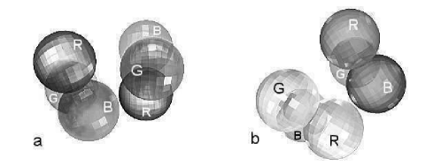
Figure 1: (a) Two combined like-charged Y-particles turned through $180^{\circ}$ with respect to one another; and (b) two coupled unlike-charged Y-particles turned through $120^{\circ}$ with respect to one another.

Similarly, in the absence of other particles two unlike-charged Y-particles will couple rotated mutually through $180^{\circ}$, forming a neutral structure. Otherwise they combine by turning clockwise through $120^{\circ}$ with respect to one another ($\uparrow$), Fig.1b, or anticlockwise ($\downarrow$), with two corresponding colour patterns:

$$\begin{vmatrix}\overline{g}_{1}&&r_{2}&\\ &\overline{b}_{1}&&g_{2}\\ \overline{r}_{1}&&b_{2}&\end{vmatrix}\text{\hskip 14.22636pt or \hskip 14.22636pt }\begin{vmatrix}\overline{g}_{1}&&b_{2}&\\ &\overline{b}_{1}&&r_{2}\\ \overline{r}_{1}&&g_{2}&\end{vmatrix}.$$ (6)

The three-colour completeness of Y permits up to three of them to combine if all of them are like-charged. These three Y will be joined in a closed loop with the following distribution of colours:

$$\begin{vmatrix}&r_{1}&&b_{2}&&g_{3}\\ b_{1}&&g_{2}&&r_{3}&\\ &g_{1}&&r_{2}&&b_{3}\end{vmatrix}\text{\hskip 14.22636pt or \hskip 14.22636pt }\begin{vmatrix}&r_{1}&&g_{2}&&b_{3}\\ b_{1}&&r_{2}&&g_{3}&\\ &g_{1}&&b_{2}&&r_{3}\end{vmatrix},$$ (7)

corresponding to the clockwise and anticlockwise mutual orientation of the components.

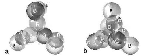
Figure 2: Three like-charged Y-particles joined with their vertices directed (a) towards the centre of the structure (left-handed state) and (b) away from the centre (right-handed state).

These structures are shown in Fig.2a, where the vertices of their Y-components are directed towards their common centre. A state with the vertices of Y directed away from their common centre is also possible (Fig.2b). The latter can be obtained from the former by mirror-reflection of all its components about the circular axis of symmetry. We shall refer to these two states as the left- and right-handed ones (3Y_L and 3Y_R). The mass of the 3Y-particle is the sum of masses of its nine preons (9 units). Similarly, its charge is 9 preon charge units. Connecting the like-coloured preons of this structure, it is seen that the spatial distribution of any particular colour appears as a helical trajectory (current) twisted along the loop. These colour-charge currents (supposedly related to the gyromagnetic properties of the structure) might be twisted clock- or anticlockwise with respect to the loop’s circular axis.

Couples of the unlike-charged Y can form chains Y$\overline{\sf Y}$ - $\overline{\sf Y}$Y - Y$\overline{\sf Y}\ldots$ with the following colour patterns:

$$\left|\begin{smallmatrix}&r_{1}&&\overline{b}_{2}\\ b_{1}&&\overline{g}_{2}&\\ &g_{1}&&\overline{r}_{2}\end{smallmatrix}\right|+\left|\begin{smallmatrix}\overline{r}_{3}&&b_{4}&\\ &\overline{g}_{3}&&r_{4}\\ \overline{b}_{3}&&g_{4}&\end{smallmatrix}\right|+\left|\begin{smallmatrix}&g_{5}&&\overline{r}_{6}\\ r_{5}&&\overline{b}_{6}&\\ &b_{5}&&\overline{g}_{6}\end{smallmatrix}\right|+\left|\begin{smallmatrix}\overline{g}_{7}&&r_{8}&\\ &\overline{b}_{7}&&g_{8}\\ \overline{r}_{7}&&b_{8}&\end{smallmatrix}\right|+\left|\begin{smallmatrix}&b_{9}&&\overline{r}_{10}\\ g_{9}&&\overline{r}_{10}&\\ &r_{9}&&\overline{b}_{10}\end{smallmatrix}\right|+\left|\begin{smallmatrix}\overline{b}_{11}&&g_{12}&\\ &\overline{r}_{11}&&b_{12}\\ \overline{g}_{11}&&r_{12}&\end{smallmatrix}\right|+\dots$$ (8)

$$\left|\begin{smallmatrix}&r_{1}&&\overline{g}_{2}\\ b_{1}&&\overline{r}_{2}&\\ &g_{1}&&\overline{b}_{2}\end{smallmatrix}\right|+\left|\begin{smallmatrix}\overline{b}_{3}&&r_{4}&\\ &\overline{r}_{3}&&g_{4}\\ \overline{g}_{3}&&b_{4}&\end{smallmatrix}\right|+\left|\begin{smallmatrix}&b_{5}&&\overline{r}_{6}\\ g_{5}&&\overline{b}_{6}&\\ &r_{5}&&\overline{g}_{6}\end{smallmatrix}\right|+\left|\begin{smallmatrix}\overline{g}_{7}&&b_{8}&\\ &\overline{b}_{7}&&r_{8}\\ \overline{r}_{7}&&g_{8}&\end{smallmatrix}\right|+\left|\begin{smallmatrix}&g_{9}&&\overline{b}_{10}\\ r_{9}&&\overline{g}_{10}&\\ &b_{9}&&\overline{r}_{10}\end{smallmatrix}\right|+\left|\begin{smallmatrix}\overline{r}_{11}&&g_{12}&\\ &\overline{g}_{11}&&b_{12}\\ \overline{b}_{11}&&r_{12}&\end{smallmatrix}\right|+\dots$$ (9)

corresponding to two ($\uparrow$ and $\downarrow$) possible states (6). The colour patterns repeat after each six consecutive ${\sf Y}\overline{\sf Y}$ groups, forming 12Y-period chains. The 12-th chain element is compatible with the first one, which makes chains to close in loops (with the 12Y-ring being the minimal-length loop).

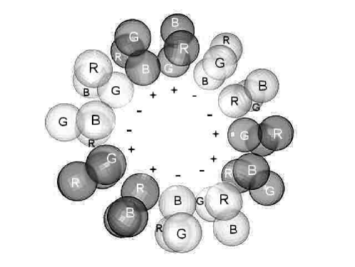
Figure 3: 12Y-structure. Mirror-reflection of all the components in the loop about the loop’s circular axis translates the structure into itself because of the equal number of Y directed with their vertices towards and outwards the centre of the structure.

The pattern (8) is visualised in Fig.3, where brighter colours are assigned to the negatively charged preons. These ring-closed chains consisting of twelve Y-particles are neutral and almost massless, according to (2) and (3). The spatial distribution of any particular colour appears as a clockwise ($\uparrow$) or anticlockwise ($\downarrow$) helix, each being a complete twist around the closed loop axis.

It is interesting to note that the mirror-reflection of all the components of 12Y about its circular axis translates the structure into itself. Thus, 12Y_L and 12Y_R are topologically indistinguishable because the number of their Y-components directed with their vertices inwards the loop coincides with the number of those directed outwards.

The 12Y-particle, consisting of 36 preons, is massless unless coupled to a charged particle, say Y or 3Y, which restores its mass. For instance, according to (3), the mass of Y^∗=Y+12Y is 39 preon mass units (3+36). The (3Y+12Y)-particle is of 45 mass units (9+36), etc. Coupling Y with 12Y and 3Y with 12Y is possible because of attractive forces arising due to the particles’ local patterns of colours and charges (analogous to the van der Waals forces between molecules). The strength and the sign of this force depends on the compatibility of colour patterns (helices) of the interacting particles. The colour pattern of 12Y_↑ does not match that of 3Y_↓. Only 3Y_↑ and 12Y_↑ or 3Y_↓ and 12Y_↓ can combine. Unlike this case, if 3Y combines with another 3Y, or 12Y with another 12Y, their helices should be opposite.

By their properties, 3Y and 12Y can be readily associated with the electron and its neutrino (leptons of the first generation). The charge of 3Y, divided by 9, gives us the conventional unit charge of the electron. Then charges of Y^∗ or 2Y^∗-particles correspond to the fractional charges of 1/3 and 2/3 (hinting at possible quark’s constituents). The Y^∗-structure cannot be free because of the strong potential of its central Y-component. It will further combine with other Y^∗. If two Y^∗-particles have likewise helix patterns, they will couple via an intermediate 12Y-particle with an opposite-helical pattern. The Y${}^{*}_{\uparrow}$ 12Y_↓ Y${}^{*}_{\uparrow}$-link can be identified with the $up$ quark. It will be charged (with a charge +3+3=+6 units) and having a mass (39+39=78 units).

Table 2: Simple preon structures. A similar table can be constructed for antipreons (with opposite charges in the third column).

Structure	Constituents	Charge	Mass
	of the	(in preon	(in preon
	structure	charge units)	mass units)
Primitive particle (preon)
$\Pi$	$1\Pi$	$-1$	1
Structures consisting of single preons
$\varrho^{-}$	$2\Pi$	$-2$	2
$g^{0}$	$1\Pi+1\overline{\Pi}$	$-1+1=0$	0
Y	$3\Pi$	$-3$	3
Second order structures consisting of preon triplets (Y-particles)
$\delta^{-}$	2Y	$-6$	6
$\gamma^{0}$	$1{\sf Y}+1\overline{\sf Y}$	$-3+3=0$	0
$e^{-}$	3Y	$-9$	9
Structures consisting of the second order substructures
$2e^{-}$	$3{\sf Y}+3{\sf Y}$	$-18$	18
$2e^{0}$	$3{\sf Y}+3\overline{\sf Y}$	$-9+9=0$	0
$\nu^{0}$	12Y	$6\times(-3+3)=0$	0
Y∗	$\nu$    +    Y	$0-3=-3$	39
$W^{-}$	$\nu$   +   $e$	$0-9=-9$	45
$u^{+}$	Y∗   $\nu$   Y∗	$+3+0+3=+6$	78
$\nu^{0}_{\mu}$	Y∗   $\nu$   $\overline{{\sf Y}}^{*}$	$-3+0+3=0$	0
$d^{-}$	$u$   +   $W$	$+6-9=-3$	123
$\mu^{-}$	$\nu_{\mu}$   +   $W$	$0-9=-9$	$(48,39)^{*}$
and so on …

*)two-component system

Being positively charged, the $up$ quark can couple to a negative particle, such as $3\overline{\sf Y}12{\sf Y}^{0}$ (with its 45 mass units and its -9 charge units). The resulting mass of $3\overline{\sf Y}12{\sf Y}^{0}$ + Y^∗ 12Y⁰ Y^∗ (the $down$ quark) is $123=45+78$, and its charge is $-3=-9+6$. Simple preon structures are summarised in Table 2.

5 The second and third generations of particles

It is natural to suppose that fermions of the second and third generations should be composed of simpler structures belonging to the first generation. For instance, the muon neutrino (a neutral particle) can be formed of unlike-charged Y^∗=Y$\nu_{e}$ and $\overline{\sf Y}^{*}=\overline{\sf Y}\nu_{e}$:

$$\nu_{\mu}={\sf Y}12{\sf Y}^{0}_{\downarrow}\ 12{\sf Y}^{0}_{\uparrow}\ 12{\sf Y}^{0}_{\downarrow}\overline{\sf Y}={\sf Y}^{*}\nu_{e}\overline{\sf Y}^{*},$$ (10)

and the muon could be structured naturally as

$$\mu=(12{\sf Y}^{0}+3\overline{\sf Y}{\sf Y})(12{\sf Y}^{0}_{\downarrow}12{\sf Y}^{0}_{\uparrow}12{\sf Y}^{0}_{\downarrow}\overline{\sf Y})=\overline{\nu}_{e}e^{-}\nu_{\mu},$$ (11)

and so on. These structures, depending on their complexity, can be rigid or non-rigid. In our model, the fermions belonging to the second and third generations are considered as clusters, rather than rigid structures (in (11) the clustered components are enclosed in parentheses). Their masses depend on the sum $M=\sum_{k}{m_{k}}$ of the masses of their components, $m_{k}$, and the sum of inverted reciprocal masses of the components, $1/m^{\prime}_{k}$: $\frac{1}{M^{\prime}}=\sum_{k}{\frac{1}{m^{\prime}_{k}}}$. The combined mass can be computed as

$$m(m_{1},m_{2},\ldots,m_{N})=MM^{\prime}=\frac{m_{1}+m_{2}+\dots+m_{N}}{1/m^{\prime}_{1}+1/m^{\prime}_{2}+\dots+1/m^{\prime}_{N}}.$$ (12)

Using this formula for fermions and comparing their computed masses with the experimental data, one can see that, for the second and third generations, the masses are reproduced with a systematic error of about 0.5% (we do not present these results here). The systematic differences must be attributed to the already mentioned simplifications in (3), as well as to the neglect of relativistic effects and dynamics of colour-charge currents responsible for the gyromagnetic properties of the structures. However, it is seen that the systematic trend depends on the number of preons in the clustered components containing 3Y and can be readily taken into account by small corrections to the masses of the clustered components as following:

$$m_{i}^{c}=m_{i}+\varkappa\eta,$$ (13)

where $m_{i}$ is the original mass of the $i$-th component (in units of the preon’s mass), $m_{i}^{c}$ is the corrected mass of the component, and $\eta$ is the correction factor:

$$\eta=\frac{1}{54\pi^{2}}\sqrt{\frac{m_{e}}{m_{e}^{c}}}.$$ (14)

$m_{e}^{c}$ is the corrected electron charge calculated from the recursive expression

$$m_{e}^{c}=m_{e}-m_{e}^{c}\eta,$$

$m_{e}^{c}$ is the corrected mass of the electron, calculated recursively by using (13); $m_{e}$ is the original electron mass, expressed in preon units ($m_{e}=9$); and $\varkappa$ is the preon factor for the given clustered component:

$$\varkappa=\left\{\begin{array}[]{ll}\frac{N^{+}}{N^{-}}m_{e},&{\rm for\hskip 5.69046ptthe\hskip 5.69046ptpositively\hskip 5.69046ptcharged\hskip 5.69046ptcomponents,\hskip 5.69046ptif\hskip 8.5359pt}Z_{system}>0\\ -N^{-},&{\rm for\hskip 5.69046ptthe\hskip 5.69046ptnegatively\hskip 5.69046ptcharged\hskip 5.69046ptcomponents,\hskip 5.69046ptif\hskip 8.5359pt}Z_{system}<0.\end{array}\right.$$

Here $N^{+}$ and $N^{-}$ are respectively the preon numbers in the positively and negatively charged clustered components. For $m_{e}=9$ and $\varkappa_{e}=-9$ the correction factor (14) is $\eta=0.001878079$ ($m_{e}^{c}=8.98313$). The constant in (14) is tuned for the best fit of the systematic trend in (12).

The fermion masses obtained with the use of (12) and (13) are summarised in Table 3. As an example, we can compute the muon’s mass. The masses of the muon’s components, according to its structure (11), are: $m_{1}=m^{\prime}_{1}=48$, $m_{2}=m^{\prime}_{2}=39$, $\varkappa=-123$, $m_{2}^{c}=38.768996$ (all in preon mass units). And the muon’s mass is

$$m_{\mu}(m_{1},m_{2}^{c})=\frac{m_{1}+m_{2}^{c}}{\frac{1}{m^{\prime}_{1}}+\frac{1}{m_{2}^{{}^{\prime}c}}}=1860.91182{\hskip 5.69046pt{\rm(preon\hskip 5.69046ptmass\hskip 5.69046ptunits)}.}$$

For the $\tau$-lepton: $m_{1}=m^{\prime}_{1}=156$, $m_{2}=m^{\prime}_{2}=201$, $\varkappa=-201$, $m_{2}^{c}=200.6227$,

$$m_{\tau}(m_{1},m_{2}^{c})=31297.1416{\hskip 5.69046pt{\rm(preon\hskip 5.69046ptmass\hskip 5.69046ptunits)}.}$$

For the proton, positively charged particle consisting of two $u-$, one $d-$quarks and a cloud of gluons $g$, masses of its components are $m_{u}=m^{\prime}_{u}=78$, $N^{+}=78$, $m_{d}=m^{\prime}_{d}=123$, $N^{-}=123$ ($m_{u}^{c}=78.0107132$). As for the gluons, only those of them should be taken into account, which, at any given moment of time, are coupled to the quarks’ preons because otherwise these gluons are massless. The total number of the coupled gluons, in accordance with the proton’s structure ($2u+d$), is $N_{g}=2N^{+}+N^{-}=279$. The mass of each gluon coupled to a preon, according to (4), is $m_{g}=1$, $m^{\prime}_{g}=\infty$. Then the resulting proton mass is

$$m_{p}=\frac{2m_{u}^{c}+m_{d}+N_{g}m_{g}}{2\frac{1}{m_{u}^{{}^{\prime}c}}+\frac{1}{m^{\prime}_{d}}+N_{g}\frac{1}{m^{\prime}_{g}}}=16525.3588{\hskip 5.69046pt{\rm(preon\hskip 5.69046ptmass\hskip 5.69046ptunits)}.}$$ (15)

Using (15), one can convert $m_{e}$, $m_{\mu}$, $m_{\tau}$ and masses of other particles from preon mass units into the proton mass units, $m_{p}$. These values are given in the fourth column of Table 3. The experimental masses of the particles (also expressed in units of $m_{p}$) are listed in the last column for comparison.

Table 3: Predicted and experimental rest masses of quarks and leptons. Values given in the third column can be converted into the proton mass units dividing them by $m_{p}=16525.3588$. Experimental masses in the last column are taken from Ref.[5] for leptons and from Ref.[6] for quarks.

Particle and		Number of active	Computed	Computed	Experimental
its structure		preons (composite	masses (preon	masses	masses
(components)		mass)	mass units)	(in $m_{p}$)	(in $m_{p}$)
First generation
$\nu_{e}$	12Y0	0	$\approx 0$	$\approx 0$	$<3\cdot 10^{-9}$
$e^{-}$	$3\overline{{\sf Y}}$	9	9	0.0005446175	0.0005446170
$u$	Y${}^{*}\nu_{e}$Y∗	78	78	0.004720019	0.0047
$d$	$u$ $\ \nu_{e}e^{-}$	123	123	0.007443106	0.0074
Second generation
$\nu_{\mu}$	Y∗   $\nu_{e}$    $\overline{{\sf Y}}^{*}$	0	$\approx 0$	$\approx 0$	$<2\cdot 10^{-4}$
$\mu^{-}$	$\nu_{\mu}$   +   $\nu_{e}e^{-}$	$m(48,39)$	1860.9118	0.11260946	0.11260951
$c$	Y∗∗   +   Y∗∗	$m(165,165)$	27122.89	1.641289	1.6
$s$	$c$    +   $e^{-}$	$m(165,165,9)$	2745.37	0.1661307	0.16
Third generation
$\nu_{\tau}$	$u$     $\nu_{e}$     $\overline{u}$	0	$\approx 0$	$\approx 0$	$<2\cdot 10^{-2}$
$\tau^{-}$	$\nu_{\tau}$    +   $\nu_{\mu}\mu^{-}$	$m(156,201)$	31297.11	1.893884	1.8939
$t$	Y∗∗∗   +   Y∗∗∗	$m(1767,1767)$	3122289	188.9392	189
$b$	$t$   +   $\mu^{-}$	$m(1767,1767,48,39)$	75813.33	4.587696	5.2

In this Table, Y^∗, Y^∗∗ and Y^∗∗∗ stand for the structures with triplets Y coupled to ring-like particles $\nu$ of increasing complexity. For instance, the electron-neutrino, $\nu_{e}=12{\sf Y}$, gives rise to a particle ${\sf Y}^{*}=\nu_{e}{\sf Y}$. Ring structures similar to that of the the electron neutrino, may be considered as “heavy neutrinos”, $\nu_{h}=12{\sf Y}^{*}$. They can further form “ultra-heavy” neutrinos $\nu_{uh}=3(\overline{\sf Y}^{*}\nu_{h}u)e^{-}$, and so on, with the number of preons increasing with the complexity of the structure. The components Y^∗∗ and Y^∗∗∗ of $c$ and $t$ may have the following structures: Y${}^{**}=u\nu_{e}u\nu_{e}e^{-}$, consisting of 165 preons, and Y${}^{***}=\nu_{uh}$Y consisting of 1767 preons.

Table 3 illustrate family-to-family similarities between the particle structures. For example, in each family, the $down$-like quark appears as a combination of the $up$-like quark, with a charged lepton belonging to the lighter family. Thus, according to this scheme, the strange-quark is composed of the charm-quark and the electron: $s=c+e^{-}$ and has a mass, $m_{s}(165,165,9)=2745.37$, resulting from $m_{c}$(165,165)=27122.89 and $m_{e}=9$. Similarly, the mass of the bottom-quark, $b=t+\mu^{-}$, is a combination of $m_{t}$(1767,1767)=3122289 with $m_{\mu}$(48,39)=1860.9118, resulting in $m_{b}(1767,1767,48,39)=75813.33$. The parentheses notation here corresponds to the abbreviated writing of (12). Each charged lepton is a combination of the neutrino from the same family with the neutrino and the charged lepton from the lighter family: $\mu^{-}=\nu_{\mu}+\overline{\nu}_{e}e^{-}$ $\tau^{-}=\nu_{\tau}+\overline{\nu}_{\mu}\mu^{-}$.

6 Conclusions

The discussed model, using the Klein-bottle topology of the universe, has reproduced the pattern of the fermion masses without using experimental input parameters. The computed masses of the charged leptons agree with experiment to an accuracy of about $10^{-6}$. The predicted masses of the quarks are also in good agreement with experiment. It is quite improbable that nine derived quantities could just spuriously agree with the seemingly random distributed experimental fermion masses. Thus, we have to conclude that the universe possesses the Klein-bottle-like topology.

References

- [1] Luminet, J.-P., Roukema, B.F., Topology of the Universe: Theory and Observations, Proc. Cargèse summer school ‘Theoretical and Observational Cosmology’, ed. Lachièze-Rey M., Netherlands, Kluwer, 117 (arXiv:astr-ph/9901364, 1998)
- [2] Roukema, B.F., On Determining the Topology of the Observable Universe via 3-D Quasar Positions, M.N. R.Astron.Soc., 283, p. 1147 (arXiv:astro-ph/9603052, 1996)
- [3] Bond, J.R., Cosmic microwave background overview, Class. and Quant. Grav., 15, p.2573 (1998)
- [4] Levin, J., Scannapieco E., Giancarlo de Gasperis, Silk, J., and Barrow, J.D, How the Universe got its spots, Class. and Quant. Grav., 15 No.9, p.2689 (arXiv:astro-ph/9807206, 1998)
- [5] Groom, D.E., et al.(Particle Data Group), Eur. Phys. Jour, C15, 1 (2000) and 2001 partial update for edition 2002, http://pdg.lbl.gov
- [6] B.R.Greene, The elegant universe, Vintage, London, 448p. (2000)
- [7] Pati, J.C. Grand Unification of Quarks and Leptons from One of Preons, in “Neutrino Physics and Astrophysics”, Erice #10, p.275 (1982)
- [8] Salam, A., Unification of Fundamental Forces, Cambridge University Press, pp.143 (1990)
- [9] Georgi, H.Q., Weinberg, S., Hierarchy of Interactions in Unified Gauge Theories, Phys.Rev.Lett, 33, p.451-454 (1974)
- [10] Dimopoulos, S., Georgi, H., in the 2nd Workshop on Grand Unification, Michigan, p.285 (1981)
- [11] Weinberg, S., Implications of Dynamical Symmetry Breaking, Phys.Rev, D 13, p.974-996 (1976)
- [12] Green, M.B., Schwartz, J.H., Witten, E., Superstring Theory, Cambridge (1987)
- [13] Donoghue, J.F., The Weight Formation Quark Masses, Phys.Rev., D 57, pp.5499-5508 (1998) (arXiv:hep-ph/9712333)
- [14] Kastrup, H.A., The contributions of Emmy Noether, Felix Klein and Sophus Lie to the modern concept of symmetries in physical systems, in “Symmetries in physics (1600-1980)”, Barcelona, pp.113-163 (1987)