Long distance contributions in $B\to K^{*}\ell^{+}\ell^{-}$ decays with polarized $K^{*}$

Abstract

We use momentum correlations as physical observables in $B\to K^{*}l^{+}l^{-}$ decays with $K^{*}$ polarized to study the long distance contributions. We show that these observables are sensitive to the scenarios of the long distance parametrizations. We find that the T-odd observable is directly related to the nonfactorizable effect in the standard model.

The study of flavor changing neutral currents (FCNCs) in B decays has an enormous progress since the CLEO observation [1] of $b\to s\gamma$. Recently, the process of $B\to Kl^{+}l^{-}$ has been also observed [2] at the Belle detector in the KEKB $e^{+}e^{-}$ storage ring. It is known that the radiative $b\to s\gamma$ and semileptonic $b\to sl^{+}l^{-}$ FCNC decays [3] in the standard model (SM) provide us with information on not only the Cabibbo-Kobayashi-Maskawa (CKM) matrix elements [4] but also physics beyond the SM. Moreover, for $b\rightarrow sl^{+}l^{-}$, new operators such as those from the box and Z-penguin diagrams can escape the strict constraint from $b\rightarrow s\gamma$ and, therefore, the new physics effect could be sizable.

In addition to the short-distance (SD) contributions, the long-distant (LD) contributions to $b\to s\gamma\ (sl^{+}l^{-})$, arising from the charm ($c$) quark pair bound states, should be taken into account. It is known that the LD effect in $b\rightarrow s\gamma$ is only a few percent and negligible, whereas it is the main part to the decay rate in $b\rightarrow sl^{+}l^{-}$. However, the parametrization of the LD contributions is not unique and has an uncertainty of about $20\%$ for the decay branching ratios (BRs) of $b\rightarrow sl^{+}l^{-}$ [5]. In order to test the SM and find new physics, it is of important to extract such theoretical uncertainty. To distinguish various theoretical parametrizations, it is interesting to see if we can find some measurable physical observables which are dominated by the LD parts.

In this paper, we will study the LD effects by considering the exclusive $B\rightarrow K^{*}l^{+}l^{-}$ decays with the polarized $K^{*}$ meson. We will define some useful observables by the momentum correlations, especially those related to T-odd operators. In a three-body decay, it is known that the simplest T-odd operator is the triple correlations given by $\vec{s}\cdot(\vec{p}_{i}\times\vec{p}_{j})$ where $\vec{s}$ is the spin vector of an outgoing particle and $\vec{p}_{i}$ and $\vec{p}_{j}$ denote any two independent momentum vectors. In terms of the CPT invariant theorem, T violation (TV) implies CP violation (CPV). Therefore, studying of T-odd observables could help us to understand the origin of CPV. We note that the T-odd observables such as the triple correlations are only associated with the imaginary parts of relevant dynamical variables. That is, even there is no weak CP phase, these observables may not vanish if a strong phase or absorptive part exists. In the SM, since the CKM matrix element of $V_{tb}V_{ts}^{*}$ involved in the process of $B\rightarrow K^{*}l^{+}l^{-}$ contains no phase, the T-odd observables can be only generated through the LD effects. Hence, these observables can be used to test the parametrizations of LD effects. In the decays of $B\rightarrow K^{*}l^{+}l^{-}$ ($l=e,\mu$, and $\tau$), the spin $s$ can be the polarized lepton, $s_{l},$ or the $K^{*}$ meson, $\epsilon^{*}(\lambda)$. For the polarized lepton, since the T-odd transverse lepton polarization flips the helicity and thus it is always associated with the lepton mass, we expect that this type of T violating effects is suppressed and less than $1\%$ for the light lepton modes [6]. Such effect is also negligible for the $\tau$ mode due to the small decay branching ratio. In this paper, we will concentrate on the light lepton modes with only $K^{*}$ polarized and set the lepton masses to be zero, i.e., $m_{l}=0$.

We start by writing the effective Hamiltonian for $b\rightarrow s\ l^{+}\ l^{-}$ as [7]

$${\cal H}=\frac{G_{F}\alpha V_{tb}V_{ts}^{*}}{\sqrt{2}\pi}\left[H_{1\mu}L^{\mu}+H_{2\mu}L^{5\mu}\right]$$ (1)

with

$$H_{1\mu} = C_{9}(\mu)\bar{s}\gamma_{\mu}(\mu)P_{L}b\ -\frac{2m_{b}}{q^{2}}C_{7}(\mu)\bar{s}i\sigma_{\mu\nu}q^{\nu}P_{R}b\,,$$

$$H_{2\mu} = C_{10}\bar{s}\gamma_{\mu}P_{L}b\,,\ \ L^{\mu}\;=\;\bar{l}\gamma^{\mu}l\,,\ \ L^{5\mu}\;=\;\bar{l}\gamma^{\mu}\gamma_{5}l\,,$$

where $C_{i}\ (i=7,9,10)$ are the Wilson coefficients (WCs) and their expressions can be found in Ref. [7] for the SM. Since the operator associated with $C_{10}$ is not renormalized under the QCD, it does not depend on the renormalization scale. As mentioned before, besides the short-distance (SD) contributions, the main effect on the BR comes from cc̄ resonant states such as $\Psi$ and $\Psi^{\prime}$. In the literature [5, 8, 9, 10, 11, 12], it has been suggested to combine the factorization assumption (FA) and vector meson dominance (VMD) approximation in estimating LD effects. As a consequence, these effects can be absorbed to the relevant WC of $C_{9}$. For comparing the different parametrizations, we adopt three scenarios in the literature for the effective WC of $C_{9}$:

(I) By defining

$$\left\langle 0\right|\bar{c}\gamma_{\mu}c\left|V(q)\right\rangle=\varepsilon_{\mu}f_{V}(q^{2})\,,$$ (2)

where $\varepsilon_{\mu}$ denotes the polarization vector of $V$, and fixing $f_{V}(q^{2})$ at the $V$ mass-shell with $q^{2}=m_{V}^{2}$, one has that

$$C_{9}^{eff}=C_{9}\left(\mu\right)+\left(3C_{1}\left(\mu\right)+C_{2}\left(\mu\right)\right)\left(h\left(x,s\right)-\frac{3}{\alpha^{2}}\sum_{V=\Psi,\Psi^{\prime}}k_{V}\frac{\pi\Gamma\left(V\rightarrow l^{+}l^{-}\right)M_{V}}{M_{V}^{2}-q^{2}-iM_{V}\Gamma_{V}}\right)\,,$$ (3)

where $h(x,s)$ describes the one-loop matrix elements of operators $O_{1}=\bar{s}_{\alpha}\gamma^{\mu}P_{L}b_{\beta}\ \bar{c}_{\beta}\gamma_{\mu}P_{L}c_{\alpha}$ and $O_{2}=\bar{s}\gamma^{\mu}P_{L}b\ \bar{c}\gamma_{\mu}P_{L}c$ [7], $M_{V}$ ($\Gamma_{V}$) are the masses (widths) of intermediate states, and the factors $k_{V}\approx 2.3$ are phenomenological parameters for compensating the approximations of the FA and VMD and reproducing the correct branching ratios $Br\left(B\rightarrow J/\Psi X\rightarrow l^{+}l^{-}X\right)=Br\left(B\rightarrow J/\Psi X\right)$ $\times$ $Br\left(J/\Psi\rightarrow l^{+}l^{-}\right)$. Here, we have neglected the small Wilson coefficients.

(II) By parametrizing $f_{V}(q^{2})$ as [5]

$$f_{V}(q^{2})=f_{V}(0)\left(1+\frac{q^{2}}{c_{V}}\left(d_{V}-h_{V}\left(q^{2}\right)\right)\right)$$ (4)

where $c_{\Psi(\Psi^{\prime})}=0.54$ $(0.77)$, $d_{\Psi(\Psi^{\prime})}=0.043$ and

$\displaystyle h_{V}\left(q^{2}\right)=\frac{1}{16\pi^{2}r}\left[-4-\frac{20r}{3}+4\left(1+2r\right)\sqrt{1-\frac{1}{r}}\arctan\frac{1}{\sqrt{1-\frac{1}{r}}}\right]$

with $r\approx q^{2}/m_{V}^{2}$ for $0\leq q^{2}\leq m_{V}^{2}$ and $f_{V}(q^{2})=f_{V}(m_{V}^{2})$ for $q^{2}>m_{V}^{2}$, one gets that

$$C_{9}^{eff}=C_{9}\left(\mu\right)+\left(3C_{1}\left(\mu\right)+C_{2}\left(\mu\right)\right)\left(h\left(x,s\right)-\frac{3}{\alpha^{2}}\sum_{V=\Psi,\Psi^{\prime}}\frac{f_{V}^{2}(q^{2})}{f_{V}^{2}(m_{V}^{2})}\frac{\pi\Gamma\left(V\rightarrow l^{+}l^{-}\right)M_{V}}{q^{2}-M_{V}^{2}-iM_{V}\Gamma_{V}}\right)\,.$$ (5)

(III) With the measurement of $R_{had}(q^{2})\equiv\sigma(e^{+}e^{-}\rightarrow hadron)/\sigma(e^{+}e^{-}\rightarrow\mu^{+}\mu^{-})$ and the dispersion relation [12], one finds that

$$C_{9}^{eff}=C_{9}\left(\mu\right)+Y^{\prime}(s)+\left(3C_{1}\left(\mu\right)+C_{2}\left(\mu\right)\right)\left({Re}\,g\left(\hat{m}_{c},s\right)+i{Im}\,g\left(\hat{m}_{c},s\right)\right)$$ (6)

where $\hat{m}_{c}=m_{c}/m_{b}$, $s=q^{2}/m_{b}^{2}$, $Y^{\prime}(s)$ is defined in Ref. [7], and

$${Re}\,g\left(\hat{m}_{c},s\right) = -\frac{8}{9}\ln\hat{m}_{c}-\frac{4}{9}+\frac{s}{3}P\int_{4\hat{m}_{\pi}^{2}}^{\infty}ds^{\prime}\frac{R_{had}^{c\bar{c}}\left(s^{\prime}\right)}{s^{\prime}\left(s^{\prime}-s\right)},$$

$${Im}\,g\left(\hat{m}_{c},s\right) = \frac{\pi}{3}R_{had}^{c\bar{c}}\left(s\right),\ \ R_{had}^{c\bar{c}}\left(s\right)\;=\;R_{cont}^{c\bar{c}}\left(s\right)+R_{res}^{c\bar{c}}\left(s\right)\,,$$

where $P$ denotes the principal value and $R_{cont}^{c\bar{c}}\left(s\right)$ and $R_{res}^{c\bar{c}}\left(s\right)$ are the contributions of continuum and resonant states with the explicit expressions given by

$$R_{cont}^{c\bar{c}}\left(s\right) = \left\{\begin{tabular}[]{lll}$0$&&for $0\leq s\leq 0.60$\\ $-6.8+11.33s$&&for $0.60\leq s\leq 0.69$\\ $1.02$&&for $0.69\leq s\leq 1,$\end{tabular}\right.$$

$$R_{res}^{c\bar{c}}\left(s\right) = \frac{9q^{2}}{\alpha^{2}}\sum_{V=\Psi,\Psi^{\prime}}k_{V}\frac{Br\left(V\rightarrow l^{+}l^{-}\right)\Gamma_{V}\Gamma_{had}^{V}}{\left(q^{2}-M_{V}^{2}\right)^{2}+M_{V}^{2}\Gamma_{V}^{2}}\,.$$

In Figure 1, we plot the real and imaginary parts of $C^{eff}_{9}$ for the three scenarios. From the figure, we clearly see that the results for $ReC^{eff}_{9}$ in (I) and (III) are close to each other and slightly different from that in (II), whereas that for $ImC^{eff}_{9}$ in (I) and (II) are almost the same but quite different from (III).

In addition, we note that the LD contributions to $BR(B\rightarrow K^{*}\gamma)$ are pure nonfactorizable effects and only at a few percent level [13], whereas they are enormous around $c\bar{c}$ resonant states for $B\rightarrow K^{*}l^{+}l^{-}$. From Ref. [14], similar to the factorizable effects to $C_{9}$, the nonfactorizable contributions to $b\rightarrow s\gamma$ can be put into $C_{7}$, given by

$$C_{7}^{eff}=C_{7}\left(\mu\right)+\omega\Delta C_{9}^{eff}\left(\mu\right)$$ (8)

with $\Delta C_{9}^{eff}\left(\mu\right)=C_{9}^{eff}\left(\mu\right)-C_{9}\left(\mu\right)$, where $\omega$ parametrizes the magnitude of the ratio of nonfactorizable and factorizable parts. By satisfying the present experimental constraint on $BR(B\rightarrow K^{*}\gamma)$ at $q^{2}=0$, we set $\omega\leq 0.15$. If the $\omega$ effect is displayed exclusively, we can directly demonstrate the magnitude of nonfactorizable effects. We also note that nonfactorizable effects in $B\to K^{*}$ decays have been computed systematically in the QCD factorization approach [15].

For $B\to K^{*}l^{+}l^{-}$ decays, the relevant transition form factors can be parametrized as

$$<K^{*}(p_{2},\epsilon)|\bar{s}\gamma_{\mu}b|\bar{B}(p_{1})> = iV(q^{2})\varepsilon_{\mu\alpha\beta\rho}\epsilon^{*\alpha}P^{\beta}q^{\rho},$$ (9)

$$<K^{*}(p_{2},\epsilon)|\bar{s}\gamma_{\mu}\gamma_{5}b|\bar{B}(p_{1})> = A_{0}(q^{2})\epsilon_{\mu}^{*}+\epsilon^{*}\cdot q\left(A_{1}(q^{2})P_{\mu}+A_{2}(q^{2})q_{\mu}\right),$$ (10)

$$<K^{*}(p_{2},\epsilon)|\bar{s}i\sigma_{\mu\nu}q^{\nu}b|\bar{B}(p_{1})> = iT(q^{2})\varepsilon_{\mu\alpha\beta\rho}\epsilon^{*\alpha}P^{\beta}q^{\rho},$$ (11)

$$<K^{*}(p_{2},\epsilon)|\bar{s}i\sigma_{\mu\nu}q^{\nu}\gamma_{5}b|\bar{B}(p_{1})> = -T_{0}(q^{2})\epsilon_{\mu}^{*}-\epsilon^{*}\cdot q\left(T_{1}(q^{2})P_{\mu}+T_{2}(q^{2})q_{\mu}\right)\,,$$ (12)

where $P=p_{1}+p_{2}$ and $q=p_{1}-p_{2}$. The correspondences between our notations and those used in the literature can be found in the Appendix of Ref. [16]. The transition amplitude for $B\rightarrow K^{*}l^{+}l^{-}$ is then obtained to be

$${\cal M}_{K^{*}}^{(\lambda)}=\frac{G_{F}\alpha_{em}V_{tb}V_{ts}^{*}}{2\sqrt{2}\pi}\left\{{\cal M}_{1\mu}^{(\lambda)}L^{\mu}+{\cal M}_{2\mu}^{(\lambda)}L^{5\mu}\right\}$$ (13)

with ${\cal M}_{1(2)\mu}^{(\lambda)}=ih_{1}(g_{1})\varepsilon_{\mu\nu\alpha\beta}\epsilon^{*\nu}(\lambda)P^{\alpha}q^{\beta}+h_{2}(g_{2})\epsilon_{\mu}^{*}(\lambda)+h_{3}(g_{3})\epsilon^{*}\cdot qP_{\mu}$ where

$$h_{1} = C_{9}^{eff}(\mu)V(q^{2})-\frac{2m_{b}}{q^{2}}C_{7}^{eff}(\mu)T(q^{2}),$$ (14)

$$h_{2} = -C_{9}^{eff}(\mu)A_{0}(q^{2})+\frac{2m_{b}}{q^{2}}C_{7}^{eff}(\mu)T_{0}(q^{2}),$$ (15)

$$h_{3} = -C_{9}^{eff}(\mu)A_{1}(q^{2})+\frac{2m_{b}}{q^{2}}C_{7}^{eff}(\mu)T_{1}(q^{2}),$$ (16)

$$g_{1} = C_{10}V(q^{2})\,,\ \ g_{2}\;=\;-C_{10}A_{0}(q^{2})\,,\ \ g_{3}\;=\;-C_{10}A_{1}(q^{2}).$$ (17)

To have a non-zero T-odd observable, the term of $\varepsilon_{\mu\nu\alpha\beta}q^{\mu}\epsilon^{*\nu}(\lambda)p_{l}^{\alpha}P^{\beta}$ is needed. To get this, we have to study the processes of $B\rightarrow K^{*}l^{+}l^{-}\rightarrow(K\pi)l^{+}l^{-}$ so that the polarizations $\lambda$ and $\lambda^{\prime}$ in the differential decay rate, written as $d\Gamma\propto H(\lambda,\lambda^{\prime})$ ${\cal M}_{K^{*}}^{(\lambda)}$ ${\cal M}_{K^{*}}^{(\lambda^{\prime})\dagger}$ with $H(\lambda,\lambda^{\prime})\equiv\epsilon(\lambda)\cdot p_{K}$ $\epsilon^{*}(\lambda^{\prime})\cdot p_{K}$, can be different. From Eq. (13), we see that ${\cal M}_{2\mu}^{(\lambda)}$ only depends on $C_{10}$. Clearly, the T violating effects can not be generated from ${\cal M}_{2\mu}^{(\lambda)}{\cal M}_{2\mu^{\prime}}^{(\lambda^{\prime})\dagger}$, but induced from ${\cal M}_{1\mu}^{(\lambda)}{\cal M}_{1\mu^{\prime}}^{(\lambda^{\prime})\dagger}$ and ${\cal M}_{1\mu}^{(\lambda)}{\cal M}_{2\mu^{\prime}}^{(\lambda^{\prime})\dagger}$. This can be understood as follows. For the ${\cal M}_{1\mu}^{(\lambda)}{\cal M}_{1\mu^{\prime}}^{(\lambda^{\prime})\dagger}TrL^{\mu}L^{\mu^{\prime}}$ contribution, the relevant T-odd terms can be roughly expressed by

$${\cal M}_{1\mu}^{(\lambda)}{\cal M}_{1\mu^{\prime}}^{(\lambda^{\prime})\dagger}TrL^{\mu}L^{\mu^{\prime}} \propto Z_{1}{Im}h_{1}h_{3}^{*}\epsilon(0)\cdot q\varepsilon_{\mu\nu\alpha\beta}q^{\mu}\epsilon^{*\nu}(\pm)p_{l^{+}}^{\alpha}P^{\beta}$$ (20)

$$+Z_{2}{Im}h_{1}h_{2}^{*}\epsilon(0)\cdot p_{l^{+}}\varepsilon_{\mu\nu\alpha\beta}q^{\mu}\epsilon^{*\nu}(\pm)p_{l^{+}}^{\alpha}P^{\beta}$$

$$+Z_{3}{Im}h_{1}h_{2}^{*}\epsilon(\mp)\cdot p_{l^{+}}\varepsilon_{\mu\nu\alpha\beta}q^{\mu}\epsilon^{*\nu}(\pm)p_{l^{+}}^{\alpha}P^{\beta}$$

where $Z_{i}\ (i=1,2,3)$ are functions of kinematic variables and independent of $C_{9}^{eff}$ and $C_{7}^{eff}$. From Eq. (17), one gets ${Im}h_{1}h_{2}^{*}\sim{Im}h_{1}h_{3}^{*}\sim{Im}C_{9}^{eff}(\mu)C_{7}^{eff}(\mu)$. We note that as shown in Eq. (20), the T-odd observables can be non-zero if the process involves a strong phase or absorptive part even without CP violating phases. Since both $C_{7,9}^{eff}(\mu)$ include the absorptive parts, the terms in Eq. (20) do not vanish in the SM. For ${\cal M}_{1\mu}^{(\lambda)}{\cal M}_{2\mu^{\prime}}^{(\lambda^{\prime})\dagger}TrL^{\mu}L^{5\mu^{\prime}}$, one gets

$$\left({\cal M}_{1\mu}^{(\lambda)}{\cal M}_{2\mu^{\prime}}^{(\lambda^{\prime})\dagger}+{\cal M}_{2\mu}^{(\lambda)}{\cal M}_{1\mu^{\prime}}^{(\lambda^{\prime})\dagger}\right)TrL^{\mu}L^{5\mu^{\prime}}\propto\left({Im}h_{2}g_{3}^{*}-{Im}h_{3}g_{2}^{*}\right)\varepsilon_{\mu\nu\alpha\beta}q^{\mu}\epsilon^{*\nu}(\pm)p_{l^{+}}^{\alpha}P^{\beta}\,.$$ (21)

From Eq. (17), we find that ${Im}h_{2}g_{3}^{*}-{Im}h_{3}g_{2}^{*}$ is only related to ${Im}C_{7}^{eff}(\mu)C_{10}^{*}$ and the dependence of ${Im}C_{9}^{eff}(\mu)C_{10}^{*}$ is canceled in Eq. (21). From Eq. (8), we see that a nonzero value of ${Im}C_{7}^{eff}(\mu)C_{10}^{*}$ in the SM is an indication of the pure nonfactorizable effect.

In order to write the differential decay rate with the $K^{*}$ polarization, we choose $\epsilon(0)=\frac{1}{m_{K^{*}}}(|\vec{p}_{K^{*}}|,0,0,E_{K^{*}})$, $\epsilon(\pm)=\left(0,1,\pm i,0\right)/\sqrt{2}$, and $p_{l^{+}}=\frac{\sqrt{q^{2}}}{2}(1,\sin\theta_{l},0,\cos\theta_{l})$ with $E_{K^{*}}=(m_{B}^{2}-m_{K^{*}}^{2}-q^{2})/2\sqrt{q^{2}}$ and $|\vec{p}_{K^{*}}|=\sqrt{E_{K^{*}}^{2}-m_{K^{*}}^{2}}$ in the $q^{2}$ rest frame and $p_{K}=(1,\sin\theta_{K}\cos\phi,\sin\theta_{K}\sin\phi,\cos\theta_{K})m_{K^{*}}/2$ in the $K^{*}$ rest frame where $\phi$ denotes the relative angle of the decaying plane between $K\pi$ and $l^{+}l^{-}$. We have that

$$\frac{d\Gamma}{d\cos\theta_{K}d\cos\theta_{l}d\phi dq^{2}}=\frac{3\alpha_{em}^{2}G_{F}^{2}\left|\lambda_{t}\right|^{2}\left|\vec{p}\right|}{2^{14}\pi^{6}m_{B}^{2}}Br(K^{*}\rightarrow K\pi)$$ (22)

$$\ \ \times\left\{4\cos^{2}\theta_{K}\sin^{2}\theta_{l}\sum_{i=1,2}\left|{\cal M}_{i}^{0}\right|^{2}+\sin^{2}\theta_{K}(1+\cos^{2}\theta_{l})\sum_{i=1,2}\left(\left|{\cal M}_{i}^{+}\right|^{2}+\left|{\cal M}_{i}^{-}\right|^{2}\right)\right.$$ (23)

$$-\sin 2\theta_{K}\sin 2\theta_{l}\sin\phi\sum_{i=1,2}{Im}\left({\cal M}_{i}^{+}-{\cal M}_{i}^{-}\right){\cal M}_{i}^{0*}-2\sin^{2}\theta_{K}\sin^{2}\theta_{l}\sin 2\phi\sum_{i=1,2}{Im}\left({\cal M}_{i}^{+}{\cal M}_{i}^{-*}\right)$$ (24)

$$\left.+2\sin 2\theta_{K}\sin\theta_{l}\sin\phi\left({Im}{\cal M}_{1}^{0}({\cal M}_{2}^{+*}+{\cal M}_{2}^{-*})-{Im}({\cal M}_{1}^{+}+{\cal M}_{1}^{-}){\cal M}_{2}^{0*}\right)\,+...\right\},$$ (25)

where $|\vec{p}|=\sqrt{(m_{B}^{2}+m_{K^{*}}^{2}-q^{2})^{2}/4m_{b}^{2}-m_{K^{*}}^{2}}$ and ${\cal M}_{i}^{0,\pm}$ denote the longitudinal and transverse polarizations of $K^{*}$, and their explicit expressions are given by

$${\cal M}_{a}^{0}=\sqrt{q^{2}}\left(\frac{E_{K^{*}}}{m_{K^{*}}}f_{2}+2\sqrt{q^{2}}\frac{\left|\vec{p}_{K^{*}}\right|^{2}}{m_{K^{*}}}f_{3}\right)\ {\rm and}\ {\cal M}_{a}^{\pm}=\sqrt{q^{2}}\left(\pm 2\left|\vec{p}_{K^{*}}\right|\sqrt{q^{2}}f_{1}+f_{2}\right)\,,$$

respectively, where $a=1(2)$ while $f=h(g)$. For simplicity, we just show the relevant terms in Eq. (25). The detailed derivation will be discussed elsewhere [17]. Other distributions for the $K^{*}$ polarization and CP violating observables can be found in Refs. [18, 19, 20]. From Eqs. (20) and (21), we know that ${Im}({\cal M}_{i}^{+}-{\cal M}_{i}^{-}){\cal M}_{i}^{0*}$ and ${Im}({\cal M}_{i}^{+}{\cal M}_{i}^{-*})$ are from ${\cal M}_{1\mu}^{(\lambda)}{\cal M}_{1\mu^{\prime}}^{(\lambda^{\prime})\dagger}TrL^{\mu}L^{\mu^{\prime}}$ while ${Im}{\cal M}_{1}^{0}({\cal M}_{2}^{+*}+{\cal M}_{2}^{-*})-{Im}({\cal M}_{1}^{+}+{\cal M}_{1}^{-}){\cal M}_{2}^{0*}$ is induced by ${\cal M}_{1\mu}^{(\lambda)}{\cal M}_{2\mu^{\prime}}^{(\lambda^{\prime})\dagger}TrL^{\mu}L^{5\mu^{\prime}}$. In Figure 2, we show the effect of the various parametrizations on the differential decay rate after integrating over angles in Eq. (25). As seen from the figure, there are not many differences among the three scenarios except the result in (II) with the LD effect. Obviously, by measuring the decay rate, one could not be able to tell which scenario of the LD parametrizations is favorable.

In order to explore the possibility of extracting LD effects, we examine the observables, defined by

$$\langle{\cal O}_{i}\rangle\equiv\int{\cal O}_{i}{\frac{d\Gamma}{dq^{2}}}$$ (26)

where ${\cal O}_{i}$ are momentum correlation operators, given by

$${\cal O}_{L} = 4\frac{\left|\vec{p}_{l^{+}}\times\vec{p}_{B}\right|^{2}}{\left|\vec{p}_{B}\right|^{2}\omega_{l^{+}}^{2}}-3\frac{\left|\vec{p}_{B}\times\vec{p}_{K}\right|^{2}}{\left|\vec{p}_{B}\right|^{2}\omega_{K}^{2}}$$ (27)

$${\cal O}_{T1} = \frac{\left(\vec{p}_{B}\cdot\vec{p}_{l^{+}}\times\vec{p}_{K}\right)\left(\vec{p}_{B}\times\vec{p}_{K}\right)\cdot\left(\vec{p}_{l^{+}}\times\vec{p}_{B}\right)}{\left|\vec{p}_{B}\right|^{3}\omega_{K}^{2}\omega_{l^{+}}^{2}}$$ (28)

$${\cal O}_{T2} = \frac{\left(\vec{p}_{B}\cdot\vec{p}_{K}\right)\left(\vec{p}_{B}\cdot\vec{p}_{l^{+}}\times\vec{p}_{K}\right)}{\left|\vec{p}_{B}\right|^{2}\omega_{K}^{2}\omega_{l^{+}}}$$ (29)

with $\omega_{K}=m_{K^{*}}/2$ and $\omega_{l^{+}}=\sqrt{q^{2}}/2$. In the $K^{*}$ rest frame, we note that ${\cal O}_{L}=4\sin^{2}\theta_{l}-3\sin^{2}\theta_{K}$, ${\cal O}_{T1}=\sin^{2}\theta_{K}\sin^{2}\theta_{l}\cos\phi\sin\phi$ and ${\cal O}_{T2}=\cos\theta_{K}\sin\theta_{K}\sin\theta_{l}\sin\phi$. Explicitly, one has that

$$\langle{\cal O}_{L}\rangle \propto \sum_{i=1,2}\left|{\cal M}_{i}^{0}\right|^{2}\,,$$ (30)

$$\langle{\cal O}_{T1}\rangle \propto \sum_{i=1,2}Im({\cal M}_{i}^{+}{\cal M}_{i}^{-*})\,,$$ (31)

$$\langle{\cal O}_{T2}\rangle \propto Im{\cal M}_{1}^{0}({\cal M}_{2}^{+*}+{\cal M}_{2}^{-*})-Im({\cal M}_{1}^{+}+{\cal M}_{1}^{-}){\cal M}_{2}^{0*}\,.$$ (32)

We note that the result from the first T-even (odd) term in Eq. (25) is similar to that from the second one. As shown in Eqs. (20) and (21), the T-odd observables of $\langle{\cal O}_{T1,T2}\rangle$ in Eq. (32) are related to ${Im}C_{9}^{eff}C_{7}^{eff*}$ and ${Im}C_{7}^{eff}C_{10}^{*}$, respectively. The statistical significances of the observables in Eq. (26) can be determined by

$$\varepsilon_{i}(q^{2})={\frac{\int{\cal{O}}_{i}{\frac{d\Gamma}{dq^{2}}}}{\sqrt{\int{\frac{d\Gamma}{dq^{2}}}\int{\cal O}_{i}^{2}{\frac{d\Gamma}{dq^{2}}}}}}\,.$$ (33)

In Figures 3 and 4, we show the statistical significances for ${\cal O}_{T1,T2}$ as functions of $s$ for various cases. From these figures, we see that: (a) the effects on the T-even observable of $\langle O_{L}\rangle$ are large and the contributions to $\varepsilon_{L}$ from scenarios (I) and (III) are slight different from (II) around the first resonance region; (b) the contributions in the scenario (III) to the T-odd observables of $\langle O_{T1,T2}\rangle$ are much smaller than the other two scenarios and those in (I) and (II) are almost the same except the region close to the first resonance; and (c) the effects of LD contributions to $\varepsilon_{T1}$ are much less than $1\%$ but those to $\varepsilon_{T2}$ are at the percent level. It is interesting to note that the differences on the results of $\langle O_{T1(2)}\rangle$ between (I,II) and (III) are significant. Moreover, it is worth to emphasize that the results of Figure 4 are purely from nonfactorizable contributions. For example, in the SM, a signal of $\varepsilon_{T2}$ will directly reflect the nonfactorized effects.

In summary, we have defined several momentum correlations as physical observables in $B\rightarrow K^{*}l^{+}l^{-}$ decays with the polarized $K^{*}$ to study the LD contributions in the SM. we have found that these observables are quite sensitive to the different scenarios of the LD parametrizations. In particular, we have illustrated that the nonfactorizable effect of $B\to J/\Psi K^{*}$ for the T-odd observable of $\langle O_{T2}\rangle$ is non-negligible. Searching for $\langle O_{T2}\rangle$ could distinguish various parametrizations of the LD contributions in exclusive heavy $B$ meson decays. Finally, we remark that if there is new physics beyond the SM, such as the leptoquark and supersymmtric models, our results here can be treated as theoretical backgrounds and the new physics contributions to observables are easily at the level of $10\%$ [17].

Acknowledgments

This work was supported in part by the National Science Council of the Republic of China under Contract Nos. NSC-90-2112-M-001-069 and NSC-90-2112-M-007-040.

    

FIG. 1.: Effective WCs of (a) $ReC^{eff}_{9}$ and (b) $ImC^{eff}_{9}$. The solid, dashed and dash-dotted lines correspond to the scenarios of (I), (II) and (III), respectively.

 

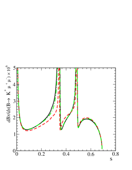
FIG. 2.: BR of $B\to K^{*}\mu^{+}\mu^{-}$ as a function of $s=q^{2}/m^{2}_{B}$. Legend is the same as Figure 1.

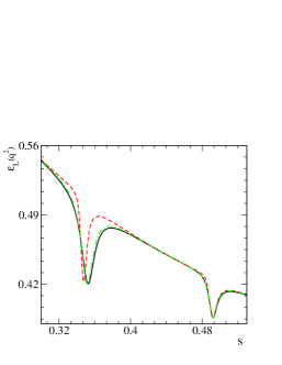
FIG. 3.: The statistical significance of $\langle{\cal O}_{L}\rangle$ as a function of $s=q^{2}/m^{2}_{B}$. Legend is the same as Figure 1.

    

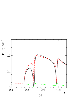
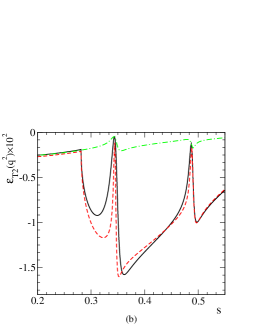
FIG. 4.: Same as Figure 3 but for (a) $\langle{\cal O}_{T1}\rangle$ and (b) $\langle{\cal O}_{T2}\rangle$ with $\omega=-0.15$.

REFERENCES

• [1] CLEO Collaboration, M. S. Alam et. al., Phys. Rev. Lett. 74, 2885 (1995).
• [2] Belle Collaboration, K. Abe et. al., Phys. Rev. Lett. 88, 021801 (2002).
• [3] For a recent review, see A. Ali et. al., Phys. Rev. D61, 074024 (2000).
• [4] N. Cabibbo, Phys. Rev. Lett. 10, 531 (1963); M. Kobayashi and T. Maskawa, Prog. Theor. Phys. 49, 652 (1973).
• [5] M. Ahmady, Phys. Rev. D53, 2843 (1996).
• [6] C.Β Q.Β Geng and C.Β P.Β Kao, Phys.Β Rev.Β D 57, 4479 (1998); C.H. Chen and C.Q. Geng, ibid. D64, 074001 (2001).
• [7] G. Buchalla, A. J. Buras and M. E. Lautenbacher, Rev. Mod. Phys 68, 1230 (1996).
• [8] N.G. Deshpande, J. Trampetic and K. Panose, Phys. Rev. D39, 1462 (1989).
• [9] C.S. Lim, T. Morozumi, and A.T. Sanda, Phys. Lett. B218, 343 (1989).
• [10] A. Ali, T. Mannel, and T. Morozumi, Phys. Lett. B273, 505 (1991).
• [11] P. O’Donnell and K. Tung, Phys. Rev. D43, R2067 (1991).
• [12] F. KrΓΌger and L.M. Sehgal, Phys. Lett. B380, 199 (1996).
• [13] A. Khodjamirian et. al., Lett. B402, 167 (1997); D. Melikhov, ibid. B516, 61 (2001).
• [14] D. Melikhov, N. Nikitin and S. Simula, Phys. Lett. B430, 332 (1998).
• [15] M.Β Beneke and T.Β Feldmann, Nucl.Β Phys.Β B 592, 3 (2001); M.Β Beneke, T.Β Feldmann and D.Β Seidel, ibid. B 612, 25 (2001).
• [16] C.H. Chen and C.Q. Geng, Phys. Rev. D63, 114025 (2001).
• [17] C.H. Chen and C.Q. Geng, hep-ph/0203003, to be published in Nucl. Phys. B.
• [18] C.S. Kim et. al., Phys. Rev. D62, 034013 (2000); C.Β S.Β Kim, Y.Β G.Β Kim and C.Β D.Β LΓΌ, ibid. D 64, 094014 (2001); T. M. Aliev et. al., Phys. Lett. B511, 49 (2001); Q.Β S.Β Yan et. al., Phys.Β Rev.Β D 62, 094023 (2000).
• [19] F.Β Kruger et. al., Phys.Β Rev.Β D 61, 114028 (2000) [Erratum-ibid.Β D 63, 019901 (2000)].
• [20] Y.Β Grossman and D.Β Pirjol, JHEP 0006, 029 (2000).
Refer to captionΒ Β Β Β Refer to caption