hep-ph/0207036 CERN–TH/2002–147 IFUP–TH/2002–17

Minimal Flavour Violation:

an effective field theory approach

G. D’Ambrosio,^a,b G.F. Giudice,^a G. Isidori,^a,c A. Strumia^a,d

^aTheoretical Physics Division, CERN, CH-1211 Genève 23, Switzerland

^bINFN, Sezione di Napoli, I-80126 Napoli, Italy

^cINFN, Laboratori Nazionali di Frascati, I-00044 Frascati, Italy

^dDipartimento di Fisica dell’Università di Pisa and INFN

Abstract

We present a general analysis of extensions of the Standard Model which satisfy the criterion of Minimal Flavour Violation (MFV). We define this general framework by constructing a low-energy effective theory containing the Standard Model fields, with one or two Higgs doublets and, as the only source of ${\rm SU}(3)^{5}$ flavour symmetry breaking, the background values of fields transforming under the flavour group as the ordinary Yukawa couplings. We analyse present bounds on the effective scale of dimension-six operators, which range between 1 and 10 TeV, with the most stringent constraints imposed by $B\to X_{s}\gamma$. In this class of theories, it is possible to relate predictions for FCNC processes in $B$ physics to those in $K$ physics. We compare the sensitivity of various experimental searches in probing the hypothesis of MFV. Within the two-Higgs-doublet scenario, we develop a general procedure to obtain all $\tan\beta$-enhanced Higgs-mediated FCNC amplitudes, discussing in particular their impact in $B\to\ell^{+}\ell^{-}$, $\Delta M_{B}$ and $B\to X_{s}\gamma$. As a byproduct, we derive some two-loop $\tan\beta$-enhanced supersymmetric contributions to $B\to X_{s}\gamma$ previously unknown.

1 Introduction

The Standard Model (SM) is a successful effective theory of particle interactions valid up to some still undetermined cut-off energy scale $\Lambda$. The goal of the search for physics beyond the SM is to find evidence for effects that are present in the theory with a finite value of $\Lambda$, but disappear in the limit $\Lambda\to\infty$. The theoretical argument based on a natural solution of the hierarchy problem requires that $\Lambda$ should not exceed few TeV, in order to stabilize the Higgs mass parameter. Experimental searches mostly provide lower bounds on $\Lambda$. Evidence for neutrino masses and limits on the proton lifetime push the effective scale of baryon and lepton number violating interactions close to the GUT scale. Limits on electron and neutron electric dipole moments require that the scale of (flavour-conserving) CP violation is larger than $10^{7}$ GeV, while the $K^{0}$–${\bar{K}}^{0}$ mass difference sets a lower bound of about $10^{6}$ GeV on the scale of $\Delta S=2$ flavour transitions. Generic contact interactions that preserve all selection rules are limited by LEP data, and their effective scales have bounds in the 1–10 TeV range.

If we insist with the theoretical prejudice that new physics has to emerge in the TeV region, then we have to conclude that the new theory is highly non-generic and we should use the lower limits on $\Lambda$ to constrain its form. In particular, $B$, $L$, and CP have to be approximate symmetries of the new theory at the TeV scale. The case of the flavour symmetry is less straightforward. Indeed the ${\rm U}(3)^{5}$ flavour symmetry of the SM gauge interactions is already broken by Yukawa couplings. Therefore, it does not seem very plausible to impose that the new interactions respect flavour, a symmetry which is not realized in the SM, i.e. in the low-energy limit of the new theory. On the other hand, generic flavour-violating interactions at $\Lambda\simeq$ TeV are experimentally excluded.

The most reasonable solution to this impasse is to impose that the effective theory respect what we call Minimal Flavour Violation (MFV). Although more rigorously defined in section 2, MFV essentially requires that all flavour and CP-violating interactions are linked to the known structure of Yukawa couplings. This concept is a familiar one in the case of supersymmetry, where this hypothesis is often adopted. In this paper we take a more general point of view: we show how the MFV hypothesis can be consistently defined independently of the structure of the new-physics model, we describe the generic form of an effective theory obeying this hypothesis, and derive the present constraints on the characteristic scale $\Lambda$. As shown in section 4, we find that the constraints vary from 1 TeV to about 10 TeV, with the strongest bound coming from $B\to X_{s}\gamma$.

In the context of MFV it is possible to relate various flavour-changing neutral current (FCNC) processes. Not only is this possible within the $B$ or $K$ systems, but one can also relate predictions for $B$ processes to $K$ rare decays. This can be achieved because, as shown in section 2, MFV implies that all flavour-changing effective operators are proportional to the same non-diagonal structure. In turn, this is a consequence of the top Yukawa coupling being much larger than all other Yukawa couplings.

An interesting novelty emerges in models in which the low-energy limit is not simply described by the SM, but it is enlarged to contain two Higgs doublets. If $\tan\beta$ (the ratio between the two vacuum expectation values) is large, then the bottom Yukawa coupling can become comparable to the top-quark coupling and the operators of the MFV effective theory contain a second non-negligible flavour-violating structure. Particularly interesting is the case in which the masses of the new Higgs bosons are smaller than $\Lambda$, since the new effects are perturbatively computable. In section 5 we derive the form of the currents coupled to the neutral and charged Higgs bosons, including all terms enhanced by $\tan\beta$ and in section 6 we discuss their phenomenological implications.

We believe that the description of flavour violations in terms of an effective theory is a useful tool to analyse future data on $B$ and $K$ mesons. When deviations from the SM predictions are observed, the comparison among various processes will indicate if they can be described in the general framework of MFV, or if they require new flavour structures. This will be a crucial hint to identify the correct theory valid above the cut-off scale $\Lambda$.

In the case of supersymmetry, the MFV hypothesis is valid when the scalar-mass soft terms are universal and the trilinear soft terms are proportional to Yukawa couplings, at an arbitrary high-energy scale. Then the physical squark masses are not equal, but the induced flavour violation is described in terms of the usual CKM parameters. In this case, the coefficients of the MFV operators described in section 3 can be perturbatively computed in terms of supersymmetric masses. However, given the large number of free parameters in a supersymmetric model, the effective-theory description can still be useful as a bookkeeping device. The concrete meaning of MFV in supersymmetric models is discussed in section 7. Moreover, in section 6 we show how the effective theory approach provides a simple systematic tool to identify $\tan\beta$-enhanced Higgs-mediated FCNC amplitudes and, using it, we identify a contribution to $B\to X_{s}\gamma$ which so far has not been discussed in the literature.

On the other hand, the effective-theory language becomes compulsory to address the flavour problem in models with non-perturbative interactions at energies $\Lambda$, like in scenarios with low-energy quantum-gravity scale. In section 7 we shall briefly discuss the natural size of the effective operators expected in some of these models.

2 Minimal Flavour Violation

The SM fermions consist of three families with two ${\rm SU}(2)_{L}$ doublets ($Q_{L}$ and $L_{L}$) and three ${\rm SU}(2)_{L}$ singlets ($U_{R}$, $D_{R}$ and $E_{R}$). The largest group of unitary field transformations that commutes with the gauge group is ${\rm U}(3)^{5}$ [1]. This can be decomposed as

$$G_{F}\equiv{\rm SU}(3)^{3}_{q}\otimes{\rm SU}(3)^{2}_{\ell}\otimes{\rm U}(1)_{B}\otimes{\rm U}(1)_{L}\otimes{\rm U}(1)_{Y}\otimes{\rm U}(1)_{\rm PQ}\otimes{\rm U}(1)_{E_{R}}~{},$$ (1)

where

$${\rm SU}(3)^{3}_{q} = {\rm SU}(3)_{Q_{L}}\otimes{\rm SU}(3)_{U_{R}}\otimes{\rm SU}(3)_{D_{R}}~{},$$ (2)

$${\rm SU}(3)^{2}_{\ell} = {\rm SU}(3)_{L_{L}}\otimes{\rm SU}(3)_{E_{R}}~{}.$$

Out of the five ${\rm U}(1)$ charges, three can be identified with baryon ($B$) and lepton ($L$) numbers and hypercharge ($Y$), which are respected by Yukawa interactions. The two remaining ${\rm U}(1)$ groups can be identified with the Peccei-Quinn symmetry of two-Higgs-doublet models [2] and with a global rotation of a single ${\rm SU}(2)_{L}$ singlet. Rearranging these two groups, we denote by ${\rm U}(1)_{\rm PQ}$ a rotation which affects only and in the same way $D_{R}$ and $E_{R}$, and by ${\rm U}(1)_{E_{R}}$ a rotation of $E_{R}$ only. The breaking of these two ${\rm U}(1)$ play an important role in flavour dynamics in models with more than one Higgs doublet, where the source of the breaking can be controlled by fields different than those that generate the Yukawa couplings. This case will be analysed in section 5.

In the SM the Yukawa interactions break the symmetry group ${\rm SU}(3)^{3}_{q}\otimes{\rm SU}(3)^{2}_{\ell}\otimes{\rm U}(1)_{\rm PQ}\otimes{\rm U}(1)_{E_{R}}$. We can formally recover flavour invariance by introducing dimensionless auxiliary fields ${Y}_{U}$, ${Y}_{D}$, and ${Y}_{E}$ transforming under ${\rm SU}(3)^{3}_{q}\otimes{\rm SU}(3)^{2}_{\ell}$ as

$${Y}_{U}\sim(3,\bar{3},1)_{{\rm SU}(3)^{3}_{q}}~{},\qquad{Y}_{D}\sim(3,1,\bar{3})_{{\rm SU}(3)^{3}_{q}}~{},\qquad{Y}_{E}\sim(3,\bar{3})_{{\rm SU}(3)^{2}_{\ell}}~{}.$$ (3)

This allows the appearance of Yukawa interactions, consistently with the flavour symmetry

$$\mathscr{L}={\bar{Q}}_{L}{Y}_{D}D_{R}H+{\bar{Q}}_{L}{{Y}_{U}}U_{R}H_{c}+{\bar{L}}_{L}{{Y}_{E}}E_{R}H{\rm~{}+~{}h.c.}~{},$$ (4)

where $H_{c}=i\tau_{2}H^{*}$ and $\langle H^{\dagger}H\rangle=v^{2}/2$, with $v=246\,{\rm GeV}$. Notice that eq. (4) describes the most general coupling of the fields ${Y}$ to renormalizable SM operators. Indeed, couplings of ${Y}$ with the kinetic terms of quarks and leptons can be eliminated with a redefinition of the fermionic fields, and Yukawa interactions with more ${Y}$ insertions can be absorbed in a redefinition of the fields ${Y}$.

Using the ${\rm SU}(3)^{3}_{q}\otimes{\rm SU}(3)^{2}_{\ell}$ symmetry, we can rotate the background values of the auxiliary fields ${Y}$ such that

$${Y}_{D}={\lambda}_{d}~{},\qquad{Y}_{L}={\lambda}_{\ell}~{},\qquad{Y}_{U}=V^{\dagger}{\lambda}_{u}~{},$$ (5)

where ${\lambda}$ are diagonal matrices and $V$ is the CKM matrix.

We define that an effective theory satisfies the criterion of Minimal Flavour Violation if all higher-dimensional operators, constructed from SM and ${Y}$ fields, are invariant under CP and (formally) under the flavour group $G_{F}$. In other words, MFV requires that the dynamics of flavour violation is completely determined by the structure of the ordinary Yukawa couplings. In particular, all CP violation originates from the CKM phase.

It is easy to realize that, since the SM Yukawa couplings for all fermions except the top are small, the only relevant non-diagonal structure is obtained by contracting two ${Y}_{U}$, transforming as $(8,1,1)$. For later convenience we define

$$(\lambda_{\rm FC})_{ij}=\left\{\begin{array}[]{ll}\left({Y}_{U}{Y}_{U}^{\dagger}\right)_{ij}\approx\lambda_{t}^{2}V^{*}_{3i}V_{3j}{}&\qquad i\not=j~{},\\ 0&\qquad i=j~{}.\end{array}\right.$$ (6)

The off-diagonal component of a generic polynomial $P({Y}_{U}{Y}_{U}^{\dagger})$ is (approximately) proportional to $\lambda_{\rm FC}$. Therefore, $\lambda_{\rm FC}$ is the effective coupling governing all FCNC processes with external down-type quarks.

3 The MFV dimension-six operators

In this section, we want to construct all possible dimension-six FCNC operators, in the context of an effective theory with MFV. For processes with external down-type quarks, three basic bilinear FCNC structures can be identified:

$${\bar{Q}}_{L}{Y}_{U}{Y}_{U}^{\dagger}Q_{L}~{},\qquad{\bar{D}}_{R}{Y}_{D}^{\dagger}{Y}_{U}{Y}_{U}^{\dagger}Q_{L}~{},\qquad{\bar{D}}_{R}{Y}_{D}^{\dagger}{Y}_{U}{Y}_{U}^{\dagger}{Y}_{D}D_{R}~{}.$$ (7)

Expanding in powers of off-diagonal CKM matrix elements and in powers of small Yukawa couplings, it is easy to realize that the only relevant bilinear FCNC structures are

$${\bar{Q}}_{L}\lambda_{\rm FC}Q_{L}\qquad{\rm and}\qquad{\bar{D}}_{R}{\lambda}_{d}\lambda_{\rm FC}Q_{L}~{}.$$ (8)

Although suppressed by ${\lambda}_{d}$, the $LR$ term has to be kept because of its unique ${\rm SU}(2)_{L}$ transformation property. Similarly to the SM case, FCNC involving external up-type quarks are absolutely negligible in this context, because of the smallness of down-type Yukawa couplings.

We are now ready to build the complete basis of gauge-invariant dimension-six FCNC operators (relevant for processes with external down-type quarks), obtained by breaking $G_{F}$ only by means of the background values of ${Y}$. Since we are interestesd also in amplitudes mediated by off-shell gauge bosons, we start writing a basis where we use the equations of motion (to reduce the number of independent terms) only on the fermion fields. The operators can be classified as follows:

• $\underline{\Delta F=2.}$ Non-negligible $\Delta F=2$ structures are of the type $({\bar{Q}}_{L}\lambda_{\rm FC}\gamma^{\mu}X^{a}Q_{L})^{2}$ where $X^{a}$ denotes either the identity or a generator of ${\rm SU}(3)_{c}\otimes{\rm SU}(2)_{L}$. In principle, these lead to four independent operators. However, once we restrict the attention to down-type quarks, by use of Fiertz identities all these structures turn out to be equivalent and we are left with a single independent term, which we choose to be

  $${\cal O}_{0}=\frac{1}{2}\left({\bar{Q}}_{L}\lambda_{\rm FC}\gamma_{\mu}Q_{L}\right)^{2}~{}.$$ (9)

• $\underline{\Delta F=1\ \mbox{Higgs field}.}$ Neglecting terms which are suppressed by quark masses via the equations of motion, we are left with the following two operators

  $${\cal O}_{H1}=i\left({\bar{Q}}_{L}\lambda_{\rm FC}\gamma_{\mu}Q_{L}\right)H^{\dagger}D_{\mu}H~{},\qquad{\cal O}_{H2}=i\left({\bar{Q}}_{L}\lambda_{\rm FC}\tau^{a}\gamma_{\mu}Q_{L}\right)H^{\dagger}\tau^{a}D_{\mu}H~{}.$$ (10)

• $\underline{\Delta F=1\ \mbox{gauge fields}.}$ The couplings of the currents (8) to the gluon field are

  $${\cal O}_{G1}=H^{\dagger}\left({\bar{D}}_{R}{\lambda}_{d}\lambda_{\rm FC}\sigma_{\mu\nu}T^{a}Q_{L}\right)G^{a}_{\mu\nu}~{},\qquad{\cal O}_{G2}=\left({\bar{Q}}_{L}\lambda_{\rm FC}\gamma_{\mu}T^{a}Q_{L}\right)D_{\mu}G^{a}_{\mu\nu}~{}.$$ (11)

  In principle, one could write similar structures for the electroweak gauge bosons. However, after the spontaneous breaking of ${\rm SU}(2)_{L}\otimes{\rm U}(1)_{Y}$, the only terms relevant for low-energy processes ($p^{2}\ll v^{2}$) are those involving the photon field, namely

  $${\cal O}_{F1}=H^{\dagger}\left({\bar{D}}_{R}{\lambda}_{d}\lambda_{\rm FC}\sigma_{\mu\nu}Q_{L}\right)F_{\mu\nu}~{},\qquad{\cal O}_{F2}=\left({\bar{Q}}_{L}\lambda_{\rm FC}\gamma_{\mu}Q_{L}\right)D_{\mu}F_{\mu\nu}~{}.$$ (12)

• $\underline{\Delta F=1\ \mbox{four-fermion operators.}}$ The operators involving leptons are

  $${\cal O}_{\ell 1}=\left({\bar{Q}}_{L}\lambda_{\rm FC}\gamma_{\mu}Q_{L}\right)({\bar{L}}_{L}\gamma_{\mu}L_{L})~{},\qquad{\cal O}_{\ell 2}=\left({\bar{Q}}_{L}\lambda_{\rm FC}\gamma_{\mu}\tau^{a}Q_{L}\right)({\bar{L}}_{L}\gamma_{\mu}\tau^{a}L_{L})~{},$$

  $${\cal O}_{\ell 3}=\left({\bar{Q}}_{L}\lambda_{\rm FC}\gamma_{\mu}Q_{L}\right)({\bar{E}}_{R}\gamma_{\mu}E_{R})~{}.$$ (13)

  The operators involving only quarks are

  $$\begin{array}[]{ll}{\cal O}_{q1}=\left({\bar{Q}}_{L}\lambda_{\rm FC}\gamma_{\mu}Q_{L}\right)({\bar{Q}}_{L}\gamma_{\mu}Q_{L})~{},&{\cal O}_{q2}=\left({\bar{Q}}_{L}\lambda_{\rm FC}\gamma_{\mu}\tau^{a}Q_{L}\right)({\bar{Q}}_{L}\gamma_{\mu}\tau^{a}Q_{L})~{},\\ {\cal O}_{q3}=\left({\bar{Q}}_{L}\lambda_{\rm FC}\gamma_{\mu}T^{a}Q_{L}\right)({\bar{Q}}_{L}\gamma_{\mu}T^{a}Q_{L})~{},&{\cal O}_{q4}=\left({\bar{Q}}_{L}\lambda_{\rm FC}\gamma_{\mu}T^{a}\tau^{b}Q_{L}\right)({\bar{Q}}_{L}\gamma_{\mu}T^{a}\tau^{b}Q_{L})~{},\\ {\cal O}_{q5}=\left({\bar{Q}}_{L}\lambda_{\rm FC}\gamma_{\mu}Q_{L}\right)({\bar{D}}_{R}\gamma_{\mu}D_{R})~{},&{\cal O}_{q6}=\left({\bar{Q}}_{L}\lambda_{\rm FC}\gamma_{\mu}T^{a}Q_{L}\right)({\bar{D}}_{R}\gamma_{\mu}T^{a}D_{R})~{},\\ {\cal O}_{q7}=\left({\bar{Q}}_{L}\lambda_{\rm FC}\gamma_{\mu}Q_{L}\right)({\bar{U}}_{R}\gamma_{\mu}U_{R})~{},&{\cal O}_{q8}=\left({\bar{Q}}_{L}\lambda_{\rm FC}\gamma_{\mu}T^{a}Q_{L}\right)({\bar{U}}_{R}\gamma_{\mu}T^{a}U_{R})~{}.\end{array}$$ (14)

The number of independent $\Delta F=1$ terms is substantially reduced once we consider the spontaneous breakdown of the gauge group, we integrate out off-shell gauge fields, and we restrict the attention to the down-type component of the terms between square brackets. This corresponds to project the ${\cal O}_{i}$ into the SM basis of FCNC operators:

$$\mathscr{H}^{\Delta F=1}_{\rm eff}=\frac{1}{\Lambda^{2}}\sum_{n}a_{n}{\cal O}_{n}~{}+~{}{\rm h.c.}\qquad\longrightarrow\qquad\frac{G_{\rm F}\alpha}{2\sqrt{2}\pi\sin^{2}\theta_{\rm W}}V^{*}_{3i}V_{3j}\sum_{n}C_{n}{\cal Q}_{n}~{}+~{}{\rm h.c.}$$ (15)

The sum on the r.h.s. of eq. (15) includes 13 terms (see appendix B), namely four QCD-penguin operators (${\cal Q}_{3\ldots 6}$), four electroweak-penguin operators (${\cal Q}_{7\ldots 10}$), magnetic and chromo-magnetic dipole operators (${\cal Q}_{7\gamma}$ and ${\cal Q}_{8G}$), and three quark-lepton operators (${\cal Q}_{9V}$, ${\cal Q}_{10A}$ and ${\cal Q}_{\nu\bar{\nu}}$). In this approach, the projection (15) defines the leading non-standard contributions to the initial conditions of the $C_{i}$ at the electroweak scale. Note that the normalization of the r.h.s.  of (15) is such that the pure electroweak contribution to the $C_{i}(M^{2}_{W})$ is of order one. Since we assumed that CP is broken only by the background values of ${Y}$, the $a_{i}$ coefficients are real.

Defining

$$\epsilon_{i}=\left(\frac{\Lambda_{0}}{\Lambda}\right)^{2}a_{i}~{},\qquad\Lambda_{0}=\frac{{\lambda}_{t}\sin^{2}\theta_{\rm W}M_{W}}{\alpha}\approx 2.4~{}{\rm TeV}~{},$$ (16)

in the case of quark-lepton and electroweak-penguin operators we find

$$\delta C_{\nu\bar{\nu}} = \epsilon_{Z}+\epsilon_{\ell 1}-\epsilon_{\ell 2}$$ (17)

$$\delta C_{10A} = \epsilon_{Z}-\epsilon_{\ell 1}-\epsilon_{\ell 2}+\epsilon_{\ell 3}$$ (18)

$$\delta C_{9V} = \epsilon_{\ell 1}+\epsilon_{\ell 2}+\epsilon_{\ell 3}-\left[(1-4\sin^{2}\theta_{\rm W})\epsilon_{Z}+2e\epsilon_{F2}\right]$$ (19)

$$\delta C_{7} = -\epsilon_{q5}+\epsilon_{q7}+\frac{1}{2N_{c}}(\epsilon_{q6}-\epsilon_{q8})-\frac{1}{2}\epsilon_{Z}+\frac{1}{2}\left[(1-4\sin^{2}\theta_{\rm W})\epsilon_{Z}+2e\epsilon_{F2}\right]$$ (20)

$$\delta C_{8} = -\frac{1}{2}(\epsilon_{q6}-\epsilon_{q8})$$ (21)

$$\delta C_{9} = -2\epsilon_{q2}+\frac{1}{N_{c}}\epsilon_{q4}+\frac{3}{2}\epsilon_{Z}+\frac{1}{2}\left[(1-4\sin^{2}\theta_{\rm W})\epsilon_{Z}+2e\epsilon_{F2}\right]$$ (22)

$$\delta C_{10} = -\epsilon_{q4}$$ (23)

where $\delta C_{i}=C_{i}(M_{W}^{2})-C_{i}^{\rm SM}(M_{W}^{2})$ and $\epsilon_{Z}=(\epsilon_{H1}+\epsilon_{H2})/2$. Some comments are in order:

• The seven combinations of $\epsilon_{i}$ appearing in eqs. (17–23) are all independent (even if the suppressed term between square brackets is neglected). This result was not obvious a priori, since the ${\cal Q}_{i}$ basis is not ${\rm SU}(2)_{L}\otimes{\rm U}(1)_{Y}$ invariant.

• The leading SM contribution to the above $C_{i}$, at the electroweak scale, can be expressed as

  $$\epsilon^{\rm SM}_{\ell 2}=\epsilon^{\rm SM}_{q2}=Z_{0}(x_{t})-\left[X_{0}(x_{t})+Y_{0}(x_{t})\right]/2~{},\qquad\epsilon^{\rm SM}_{\ell 1}=\left[X_{0}(x_{t})-Y_{0}(x_{t})\right]/2~{},$$

  $$\epsilon^{\rm SM}_{Z}=Z_{0}(x_{t})~{},\qquad\epsilon^{\rm SM}_{F2}=\epsilon^{\rm SM}_{\ell 3}=\epsilon^{\rm SM}_{q3\ldots q8}=0~{},$$

  where $X$, $Y$ and $Z$ are the ${\cal O}(1)$ loop functions defined as in [3]. Thus, in general, the non-standard contributions cannot be re-absorbed into a redefinition of the SM electroweak contributions.

• Since the $\epsilon_{i}$ appear with ${\cal O}(1)$ coefficients in eqs. (17–23), an experimental determination of the parameters $C_{i}$, at the weak scale, with a precision $p$, allow, in general, to set bounds of ${\cal O}(\Lambda_{0}/\sqrt{p})$ on the effective scale of dimension-six operators. Thus precision experiments on rare decays could aim to probe effective scales of new physics up to $\sim 10$ TeV, within MFV models.

• The seven independent combinations appearing in eqs. (17–23) could be determined by experimental data on one type of $d_{i}\to d_{j}$ amplitudes only. Then the MFV hypothesis could be tested by comparing different types of FCNC transitions (namely $b\to d$, $b\to s$ and $s\to d$).

In the case of $C_{3\ldots 6}$ the SM contribution is strongly enhanced by QCD and is likely to obscure any effect of the $\epsilon_{i}$, if these are ${\cal O}(1)$ or smaller. On the other hand, the $\epsilon_{i}$ have a potential non-negligible impact on the initial conditions of dipole operators,

$$\delta C_{7\gamma}=\frac{2g^{2}}{e}\epsilon_{F1}~{},\qquad\qquad\delta C_{8G}=\frac{2g^{2}}{g_{s}}\epsilon_{G1}~{},$$ (24)

whose SM contributions are

$$C^{\rm SM}_{7\gamma}(M_{W}^{2})=-\frac{1}{2}D^{\prime}_{0}(x_{t}),\qquad\qquad C^{\rm SM}_{8G}(M_{W}^{2})=-\frac{1}{2}E^{\prime}_{0}(x_{t})~{}.$$

The loop functions $D^{\prime}_{0}$ and $E^{\prime}_{0}$ are given in [3]. The last term needed for a complete analysis of the flavour sector is the universal modification of $\Delta F=2$ amplitudes. This leads to

$$\delta C_{0}=2\epsilon_{0}~{},$$ (25)

where

$$\mathscr{H}^{\Delta F=2}_{\rm eff}=\frac{G^{2}_{F}M_{W}^{2}}{8\pi^{2}}(V^{*}_{3i}V_{3j})^{2}C_{0}\left[\bar{d}_{i}\gamma_{\mu}(1-\gamma_{5})d_{j}\right]^{2}~{},$$ (26)

so that $C_{0}^{\rm SM}(M_{W}^{2})=S_{0}(x_{t})/2$ [3].

In conclusion, the leading non-standard FCNC effects in (one-Higgs doublet) models with MFV can be described in terms of the ten independent $\epsilon_{i}$ combinations appearing in eqs. (17)–(25).

4 Experimental bounds

$$\begin{array}[]{rlc|ccc}\lx@intercol\hfil\hbox{Minimally flavour violating}\hfil\lx@intercol&\hbox{main}&\lx@intercol\hfil\Lambda\hbox{ [TeV]}\hfil\lx@intercol&\\ \lx@intercol\hfil\hbox{dimension~{}six~{}operator}\hfil\lx@intercol&\hbox{observables}&-&+\\ \hline\cr{\cal O}_{0}=&\frac{1}{2}(\bar{Q}_{L}\lambda_{\rm FC}\gamma_{\mu}Q_{L})^{2}\phantom{X^{X^{X}}}&\epsilon_{K},\quad\Delta m_{B_{d}}&6.4&5.0\\ {\cal O}_{F1}=&H^{\dagger}\left({\bar{D}}_{R}{\lambda}_{d}\lambda_{\rm FC}\sigma_{\mu\nu}Q_{L}\right)F_{\mu\nu}&B\to X_{s}\gamma&9.3&12.4\\ {\cal O}_{G1}=&H^{\dagger}\left({\bar{D}}_{R}{\lambda}_{d}\lambda_{\rm FC}\sigma_{\mu\nu}T^{a}Q_{L}\right)G^{a}_{\mu\nu}&B\to X_{s}\gamma&2.6&3.5\\ {\cal O}_{\ell 1}=&(\bar{Q}_{L}\lambda_{\rm FC}\gamma_{\mu}Q_{L})(\bar{L}_{L}\gamma_{\mu}L_{L})&B\to(X)\ell\bar{\ell},\quad K\to\pi\nu\bar{\nu},(\pi)\ell\bar{\ell}&3.1&2.7&*\\ {\cal O}_{\ell 2}=&({\bar{Q}}_{L}\lambda_{\rm FC}\gamma_{\mu}\tau^{a}Q_{L})({\bar{L}}_{L}\gamma_{\mu}\tau^{a}L_{L})&B\to(X)\ell\bar{\ell},\quad K\to\pi\nu\bar{\nu},(\pi)\ell\bar{\ell}&3.4&3.0&*\\ {\cal O}_{H1}=&(\bar{Q}_{L}\lambda_{\rm FC}\gamma_{\mu}Q_{L})(H^{\dagger}iD_{\mu}H)&B\to(X)\ell\bar{\ell},\quad K\to\pi\nu\bar{\nu},(\pi)\ell\bar{\ell}&1.6&1.6&*\\ {\cal O}_{q5}=&(\bar{Q}_{L}\lambda_{\rm FC}\gamma_{\mu}Q_{L})(\bar{D}_{R}\gamma_{\mu}D_{R})&B\to K\pi,\quad\epsilon^{\prime}/\epsilon,\ldots&\lx@intercol\hfil\sim 1\hfil\lx@intercol\\ \end{array}$$

Table 1: Bounds on MFV operators. The SM is extended by adding minimally flavour-violating dimension-six operators with coefficient $\pm 1/\Lambda^{2}$ ($+$ or $-$ denote their constructive or destructive interference with the SM amplitude). Here we report the bounds at $99\%$ CL on $\Lambda$, in $\,{\rm TeV}$, for the single operator (in the most representative cases). Fine-tuned scenarios with small $\Lambda$, such that new physics flips the sign of the SM amplitude are not reported (see text). The $*$ signals the cases where a significant increase in sensitivity is expected in the near future.

         

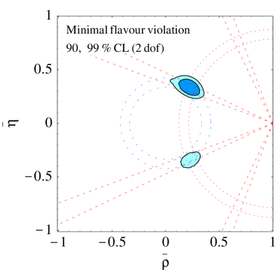
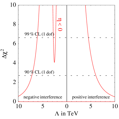
Figure 1: Fit of $\Delta F=2$ data in MFV models. Left: fit of $\bar{\rho}$ and $\bar{\eta}$ in models with minimal flavour violation. The dotted lines denotes 68% CL intervals imposed by the observables insensitive to $|C_{0}(M_{W}^{2})|$, namely $|V_{ub}|$, $\Delta M_{B_{d}}/\Delta M_{B_{s}}$ and $a^{CP}_{\Psi K}$. Input values are shown in table 2. Right: $\Delta\chi^{2}$ of the global CKM fit as a function of the scale of the operator ${\cal O}_{0}$.

$$\begin{array}[]{rcll}m_{t}(m_{t})&=&(166.8\pm 5.1)\,{\rm GeV}&\hbox{running top masss}\\ m_{b}(m_{b})&=&(4.23\pm 0.07)\,{\rm GeV}&\hbox{running bottom masss}\\ m_{c}(m_{c})&=&(1.3\pm 0.1)\,{\rm GeV}&\hbox{running charm masss}\\ \alpha_{\rm s}(M_{Z})&=&0.119\pm 0.003&\hbox{strong coupling}\\ \Delta M_{B_{d}}&=&(0.487\pm 0.014)/\hbox{ps}&\hbox{$B_{d}$ mass difference}\\ \lambda&=&0.2237\pm 0.0033&\hbox{Cabibbo angle}\\ A&=&0.819\pm 0.035&\hbox{Wolfenstein $A$ parameter}\\ \left|V_{ub}/V_{cb}\right|&=&0.0865\pm 0.0094&\hbox{ratio of CKM mixings}\\ a^{CP}_{\Psi K}&=&0.732\pm 0.063&\hbox{CP-violation in $B_{d}\to\Psi K$ \cite[cite]{[\@@bibref{}{sin2b}{}{}]}}\\ \hline\cr f_{B_{d}}B_{B_{d}}^{1/2}&=&(0.230\pm 0.025)\,{\rm GeV}&\hbox{Matrix element for $B_{d}$ mixing}\\ \xi&=&1.14\pm 0.04&\hbox{Relative matrix element for $B_{s}$ vs $B_{d}$ mixing}\\ B_{K}&=&0.87\pm 0.06&\hbox{matrix element for $K$ mixing}\\ \eta_{1}&=&1.38\pm 0.25&\hbox{RGE factor for $cc$-induced $K$ mixing}\\ \eta_{2}&=&0.57\pm 0.01&\hbox{RGE factor for $tt$-induced $K$ mixing}\\ \eta_{3}&=&0.47\pm 0.04&\hbox{RGE factor for $ct$-induced $K$ mixing}\\ \eta_{B}&=&0.55\pm 0.01&\hbox{RGE factor for $B$ mixing}\\ \end{array}$$

Table 2: Data used to produce the CKM fit in fig. 1. The probability distribution of $\Delta M_{B_{s}}$, as well as input values not reported above, are taken from [5].

4.1 $\Delta F=2$ and the CKM fit

In generic models with MFV, the CKM matrix can still be determined with good accuracy [6, 7]. Employing the improved Wolfenstein parametrization [8], $\lambda$ and $A$ are completely determined by tree-level processes and only $\bar{\rho}$ and $\bar{\eta}$ are potentially affected by new physics. The data used to constrain $\bar{\rho}$ and $\bar{\eta}$ are $|V_{ub}|$, determined from a tree-level transition, $\Delta M_{B_{d}}/\Delta M_{B_{s}}$, $a^{CP}_{J/\Psi K}$, $\Delta M_{B_{d}}$ and $\epsilon_{K}$, which are sensitive to $\Delta F=2$ amplitudes. If the modification of $\Delta F=2$ amplitudes is induced only by the operator ${\cal O}_{0}$ in eq. (9), then the ratio $\Delta M_{B_{d}}/\Delta M_{B_{s}}$ remains unchanged and the relation between $a^{CP}_{\Psi K}$ and $\sin(2\beta)$ can only be modified by an overall sign [7].

In fig. 1 (left) we show the result of a $\bar{\rho}$–$\bar{\eta}$ fit where $C_{0}(M_{W}^{2})$, or the Wilson coefficient of ${\cal O}_{0}$ at the electroweak scale, is treated as a free parameter. As can be noted, in addition to the standard solution with $\bar{\eta}>0$, also a solution with $\bar{\eta}<0$ appears. The latter arises from the fine-tuned scenario where $C_{0}(M_{W}^{2})$ is about equal in magnitude to the SM case but has the opposite sign. The solution with $\bar{\eta}<0$ is somewhat disfavoured, as can be more precisely seen in the right panel of fig. 1. In fact, while the SM contribution to $\epsilon_{K}$ proportional to the charm mass cannot be neglected because is enhanced by infra-red logarithms, the new physics contribution to $\epsilon_{K}$ is dominated by the top, see eq. (6). This breaks the $(C_{0},\bar{\eta})\leftrightarrow(-C_{0},-\bar{\eta})$ symmetry of all other observables.

The low-quality solution with $\bar{\eta}<0$ is obtained for $\Lambda\approx\Lambda_{0}$. Barring this fine-tuned possibility, the results in fig. 1 can be translated into a bound on the effective scale of the non-standard $\Delta F=2$ operator, reported in the first row of table 1. It will be difficult to improve these bounds in the near future, because hadronic uncertainties on the matrix elements of $\Delta S=2$ and $\Delta B=2$ operators are the main limiting factor. Even with ${\cal O}(1\%)$ experimental uncertainties on $a^{CP}_{\Psi K}$ and $\Delta M_{B_{d}}/\Delta M_{B_{s}}$, the $\Delta F=2$ bounds on $\Lambda$ will remain below 10 TeV as long as the theoretical errors on the matrix elements will remain above $10\%$. The constraint from $|V_{ub}/V_{cb}|$ (circle centered on the origin) around the best fit regions is consistent and tangent to the constraint from $a^{CP}_{\Psi K}$ (rays originating from $\bar{\rho}=1$), and therefore has little impact in the global fit.

4.2 $B\to X_{s}\gamma$

The inclusive rare decay $B\to X_{s}\gamma$ provides, at present, the most stringent bound on the effective scale of the new FCNC operators. Taking into account the new precise measurements reported by CLEO [9], Belle [10], and Babar [11] the world average is

$${\cal B}(B\to X_{s}\gamma)=(3.46\pm 0.34)\times 10^{-4}~{},$$ (27)

to be compared with the SM expectation [12]

$${\cal B}(B\to X_{s}\gamma)_{\rm SM}=(3.73\pm 0.30)\times 10^{-4}~{}.$$ (28)

As is well known, NLO QCD corrections play a rather important role in this process. For this reason, we will assume that $\delta C_{7\gamma,8G}$, defined in eq. (16), describe the deviations of $C_{7\gamma,8G}^{\rm NLO}(M_{W}^{2})$ from their SM values, although this is formally not correct since QCD corrections to the new effective operators have not been included. The full NLO expression for ${\cal B}(B\to X_{s}\gamma)$ (see refs. [12, 13, 14]), used in our numerical computation, can be approximated as

$$\frac{{\cal B}(B\to X_{s}\gamma)}{{\cal B}(B\to X_{s}\gamma)_{\rm SM}}=1-2.4\delta C_{7\gamma}-0.7\delta C_{8G}+{\cal O}(\delta C^{2})~{}.$$ (29)

Since the error in eq. (28) is largely dominated by low-energy dynamics (in particular by the value of $m_{c}$), we ignore the correlations between ${\cal B}(B\to X_{s}\gamma)_{\rm SM}$ and the coefficients on the r.h.s. of eq. (29). Combining all errors in quadrature and setting, alternatively, $\delta C_{8G}=0$ or $\delta C_{7\gamma}=0$, we obtain the fits shown in fig. 2 and the bounds reported in table 1. Also in this case there is a particular value of $\Lambda$ for which we obtain the condition $C_{7\gamma}(m_{b})\approx-C_{7\gamma}^{\rm SM}(m_{b})$, allowed by data. This corresponds to the sharp peaks shown in fig. 2, located at $\Lambda\approx 3$ TeV for ${\cal O}_{F1}$ and $\Lambda\approx 1$ TeV for ${\cal O}_{G1}$.

         

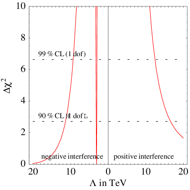
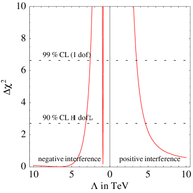
Figure 2: Bounds on the scale of the operators ${\cal O}_{F1}$ (left) and ${\cal O}_{G1}$ (right) from $B\to X_{s}\gamma$.

In presence of both $\delta C_{8G}\not=0$ and $\delta C_{7\gamma}\not=0$ there can be cancellations between their effects, giving rise to two allowed bands for their coefficients. When studying processes related to $b\to s\gamma$, such as $b\to s\bar{\ell}\ell$, one has to keep in mind that the effective constraint is that the renormalized coefficient $|C_{7\gamma}(m_{b})|$ must be very close to the its SM value.

It is interesting to compare the limits on the effective scale of ${\cal O}_{F1}$ with limits on flavour-diagonal dipole-type operators. Since we assumed no new sources of CP violation, we get no useful bounds from electric-dipole moments. On the other hand, the anomalous magnetic moment of the muon does provide a bound on the operator $eH^{\dagger}\left(\bar{E}_{R}{\lambda}_{\ell}\sigma_{\mu\nu}L_{L}\right)F_{\mu\nu}$. Taking into account theoretical and experimental uncertainties, the limit on its effective scale is around 2 TeV, much weaker than in the $B\to X_{s}\gamma$ case.

We finally note that in this approach the stringent constraints from $B\to X_{s}\gamma$ can directly be translated into bounds on non-standard effects in $s\to d\gamma$ and $b\to d\gamma$ transitions. The former could in principle tested by CP-asymmetries in $K\to\pi\pi\gamma$ decays [15]. However, due long-distance contaminations, only an order-of-magnitude enhancement of the short-distance amplitude could eventually be seen in $K\to\pi\pi\gamma$: the constraint from $B\to X_{s}\gamma$ implies this cannot occur in MFV models. More promising from the experimental point of view is the inclusive $B\to X_{d}\gamma$ rate, whose bound in MFV models is shown in table 3.

$$\begin{array}[]{l|lc|l}\hbox{Observable }&\hbox{99(90)\% MFV limit}\!\!\!\!\!\!&\ \ \hbox{determined by}&\hbox{90\% exp. limit ~{}\cite[cite]{[\@@bibref{}{PDG}{}{}]}}\\ \hline\cr{\cal B}(B\to X_{d}\gamma)&2(2)\times 10^{-5}&{\cal B}(B\to X_{s}\gamma)&-\\ \hline\cr{\cal B}(B\to X_{s}\nu\bar{\nu})&8(6)\times 10^{-4}&&6.4\times 10^{-4}\\ {\cal B}(B\to X_{d}\nu\bar{\nu})&3(2)\times 10^{-5}&{\cal B}(K^{+}\to\pi^{+}\nu\bar{\nu})&-\\ {\cal B}(K_{L}\to\pi^{0}\nu\bar{\nu})&5(4)\times 10^{-10}&&5.9\times 10^{-7}\\ \hline\cr{\cal B}(B_{s}\to\tau^{+}\tau^{-})&4(3)\times 10^{-6}&&-\\ {\cal B}(B_{d}\to\tau^{+}\tau^{-})&1(1)\times 10^{-7}&{\cal B}(B\to X_{s}\bar{\ell}\ell)&-\\ {\cal B}(B_{s}\to\mu^{+}\mu^{-})&2(1)\times 10^{-8}&[{\cal B}(K_{L}\to\mu^{+}\mu^{-})_{\rm short}]{}&2.0\times 10^{-6}\\ {\cal B}(B_{d}\to\mu^{+}\mu^{-})&6(5)\times 10^{-10}&&2.0\times 10^{-7}\quad\cite[cite]{[\@@bibref{}{Babar_mm}{}{}]}\\ {\cal B}(K_{L}\to\pi^{0}e^{+}e^{-})_{\rm CP-dir}&2(2)\times 10^{-11}&&5.6\times 10^{-10}\\ \end{array}$$

Table 3: Bounds on various decay rates obtained in MFV models with one Higgs doublet.

4.3 Rare FCNC decays into a lepton pair

These processes provide constraints on the three Wilson coefficients $C_{\nu\bar{\nu}}$, $C_{9V}$ and $C_{10A}$ which, in turn, receive non-standard contributions from ${\cal O}_{H1,H2}$, ${\cal O}_{F1,F2}$ and ${\cal O}_{\ell 1\ldots\ell 3}$, as shown in eqs. (17)–(19). The simplest cases are the decays into a neutrino pair, sensitive only to $C_{\nu\bar{\nu}}$, or the helicity suppressed pure-leptonic decays [$K_{L}(B)\to\ell^{+}\ell^{-}$], sensitive only to $C_{10A}$.

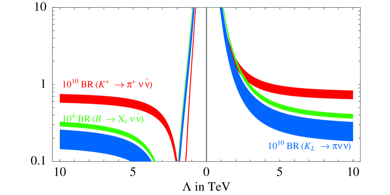
Figure 3: Branching ratios of various processes involving $d_{i}\to d_{j}\nu\bar{\nu}$ transitions as functions of the scale of the effective operator ${\cal O}_{\ell 1}$. The bands represent $1\sigma$ uncertainties, taking into account the present determination of the CKM parameters.

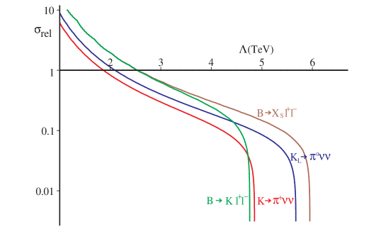
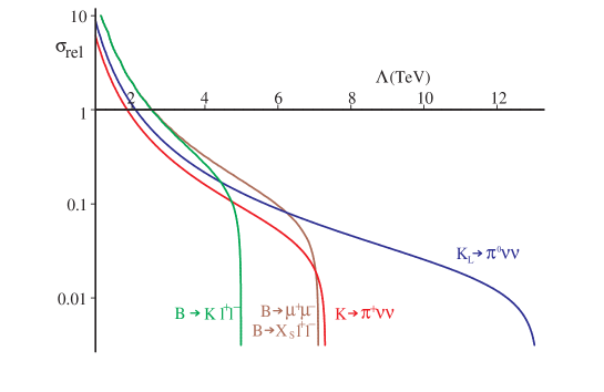
Figure 4: Comparison of the effectiveness of different rare modes in setting future bounds on the scale of the operator ${\cal O}_{\ell 1}$. The vertical axis indicates the relative precision of an hypothetic measurement of the rate, with central value equal to the SM expectation. The curves in the two panels are obtained assuming an uncertainty of 10% (left) or 1% (right) on the corresponding overall CKM factor (e.g. $|V_{tb}^{*}V_{td}|^{2}$ in the case of $B_{d}\to\mu^{+}\mu^{-}$).

Concerning $\nu\bar{\nu}$ modes, the most significant bounds come from ${\cal B}(K^{+}\to\pi^{+}\nu\bar{\nu})$. Using the SM expression of this observable [18] and treating $C_{\nu\bar{\nu}}$ as a free parameter, the recent E787 result [19]

$${\cal B}(K^{+}\to\pi^{+}\nu\bar{\nu})=\left(1.57^{~{}+~{}1.75}_{~{}-~{}0.82}\right)\times 10^{-10}~{}.$$ (30)

leads to the $99\%$ CL limit

$$-4.8<C_{\nu\bar{\nu}}/C^{\rm SM}_{\nu\bar{\nu}}<4.0~{}.$$ (31)

These bounds are still rather weak, corresponding to effective scales of the new physics operator around 1 TeV, nonetheless they already imply significant bounds on ${\cal B}(K_{L}\to\pi^{0}\nu\bar{\nu})$ and ${\cal B}(B\to X_{s}\nu\bar{\nu})$, as shown in table 3 (see also ref. [20]). In few years, at the end of the E949 experiment, assuming that the central value of ${\cal B}(K^{+}\to\pi^{+}\nu\bar{\nu})$ will move towards the SM prediction, we can expect to probe $\Lambda$ from this observable up to about $3$ TeV, a sensitivity comparable to the one of electroweak precision data on the corresponding flavour-diagonal terms. At the end of the CKM experiment, with a $10\%$ measurement of this branching ratio, the search on $\Lambda$ could be pursued up to above 5 TeV. As illustrated in fig. 4, a sensitivity above 10 TeV could in principle be reached by a measurement of ${\cal B}(K_{L}\to\pi^{0}\nu\bar{\nu})$ with a precision of few percent around the SM value, since this rate is free from the theoretical uncertainty due to charm contributions.

The most interesting constraint on pure-leptonic decays is provided by $K_{L}\to\mu^{+}\mu^{-}$. The branching ratio of this decay is measured very precisely; however, this mode receives also a large long-distance amplitude by the two-photon intermediate state. Actually short- and long-distance dispersive parts cancel each other to a good extent, since the total $K_{L}\to\mu^{+}\mu^{-}$ rate is almost saturated by the absorptive two-photon contribution. Taking into account the recent experimental result on ${\cal B}(K_{L}\to\mu^{+}\mu^{-})$ [21] and following the analyses of the long-distance amplitude in [22], we shall impose the conservative upper bound

$${\cal B}(K_{L}\to\mu^{+}\mu^{-})^{\rm short}\leq 3.0\times 10^{-9}~{},$$ (32)

that we shall treat as an absolute limit. Employing the SM expression of ${\cal B}(K_{L}\to\mu^{+}\mu^{-})^{\rm short}$ [3] and taking into account the uncertainty of the CKM fit, this information can be translated into the $99\%$ CL limit

$$-3.2<C_{10A}/C^{\rm SM}_{10A}<2.6~{}.$$ (33)

We then conclude that the present level of precision reached by $K_{L}\to\mu^{+}\mu^{-}$ and $K^{+}\to\pi^{+}\nu\bar{\nu}$ is comparable, although the bounds from the former process are still more stringent. However, it should stressed that in the $K_{L}\to\mu^{+}\mu^{-}$ case the limiting error is theoretical and very difficult to substantially improve in the near future.

Differential rate and forward-backward asymmetries in $B\to X_{s}\ell^{+}\ell^{-}$ offer, in principle, the possibility to disentangle the contributions of both $C_{9V}$ and $C_{10A}$, as well as their relative sign with $C_{7\gamma}$ [23]. Experiments are still far from such a detailed analysis, nonetheless recent data from Belle [24] and Babar [25] already start to provide significant constraints on these coefficients. Referring to [26] for a detailed discussion of the interplay of the various measurements, here we shall limit to analyse the consequences of the most interesting result, namely

$${\cal B}(B\to K\ell^{+}\ell^{-})=(0.76\pm 0.19)\times 10^{-6}~{}\cite[cite]{[\@@bibref{}{Belle_rare,Babar_rare}{}{}]}~{}.$$ (34)

Employing the $B\to K$ form factors in [27], the $B\to K\ell^{+}\ell^{-}$ rate can be fitted using the following approximate expression

$${\cal B}(B\to K\ell^{+}\ell^{-})=\left[2.8(1.0-\delta C_{10A})^{2}+2.7(1.1+\delta C_{9V}\pm 0.13)^{2}\right]\times 10^{-7}~{},$$ (35)

where the overall normalization is affected by a $30\%$ theoretical uncertainty. The $\pm$ term in eq. (35) corresponds to the small contribution of $C_{7}(m_{b})$, after the $B\to X_{s}\gamma$ constraint has been imposed (the negative sign corresponds to the SM solution). Setting to zero the vector contribution (i.e. in the most conservative scenario) we find a $99\%$ CL bound on $C_{10A}$ slightly more stringent than in eq. (33):

$$-2.3<C_{10A}/C^{\rm SM}_{10A}<2.3~{}.$$ (36)

Given the important role of hadronic uncertainties in the derivation of both eq. (36) and eq. (33), we do not combine these two constraints on $C_{10A}$: the MFV bounds on $B\to\ell^{+}\ell^{-}$ reported in table 3 are obtained from eq. (36) only. Using eqs. (34)–(35) we also derived a rather stringent bound on the direct-CP-violating contribution to $K_{L}\to\pi^{0}e^{+}e^{-}$, sensitive both to $C_{9V}$ and $C_{10A}$ [3].

The constraints on $C_{\nu\bar{\nu}}$, $C_{10A}$ and $C_{9V}$ can finally be combined to derive significant bounds on the effective scale of the dimension-six operators ${\cal O}_{H1,H2}$ and ${\cal O}_{\ell 1\ldots\ell 3}$. We report in table 1 the results of three representative cases: $O_{H1}$, which modifies in the same way $C_{\nu\bar{\nu}}$ and $C_{10A}$, leaving $C_{9V}$ almost unaffected; $O_{\ell 2}$, which increases or decreases simultaneously the three coefficients; $O_{\ell 1}$, which acts constructively on $C_{10A,9V}$ and destructively on $C_{\nu\bar{\nu}}$, or viceversa (the first possibility is reported under the + sign in table 1).

Focusing on $d_{i}\to d_{j}\nu\bar{\nu}$ transitions, we plot in fig.  3 the predicted rates for the $K^{+}\to\pi^{+}\nu\bar{\nu}$, $K_{L}\to\pi^{0}\nu\bar{\nu}$ and $B\to X_{s}\nu\bar{\nu}$ decay rates in presence of the ${\cal O}_{\ell 1}$ operator. The left and right panels correspond to destructive and constructive interference with the SM contribution. The bands show the present one standard deviation uncertainty, combining all errors in quadrature. Improved determinations of the CKM parameters will make the predictions more precise. Since these modes are all affected by the same combination of effective operators, the presence of other operators, such as ${\cal O}_{H1}$ or ${\cal O}_{\ell 2}$, induces only a rescaling of the horizontal axis.

In view of future precise measurements of rare modes, in fig. 4 we compare the effectiveness of different channels in setting bounds on the scale of ${\cal O}_{\ell 1}$. This figure should be taken with some care since the bounds strongly depend on the central values of the measurements (here assumed to coincide with SM expectations) and the comparison is modified in presence of additional operators. However, some interesting conclusions can still be drawn. For instance, it is clear that in the short term an important rôle will be played by $B\to X_{s}\ell^{+}\ell^{-}$: a $10\%$ measurement of this rate — within the reach of $B$ factories — should lead to bounds on $\Lambda$ up to above 5 TeV. On the other hand, $K_{L}\to\pi^{0}\nu\bar{\nu}$ is probably the most interesting channel in a long-term perspective.

4.4 Non-leptonic decays

In principle also non-leptonic $B$ and $K$ decays could be used to put constrains on MFV operators: to obtain significant bounds it is necessary to disentangle the tiny contribution of electroweak operators (${\cal Q}_{7\ldots 10}$) from the dominant effects due to tree-level and gluon-penguin amplitudes (described by ${\cal Q}_{1\ldots 6}$). Penguin-dominated $B$ decays, such as $B\to K\pi$, seems the most promising candidates for this program. However, theoretical and experimental uncertainties are still quite large and do not allow to extract competitive bounds at the moment.

Hadronic uncertainties are drastically reduced in CP-violating time-dependent asymmetries, such as $a^{CP}_{\Psi K}$. However, in the MFV scenario we do not expect significant effects on these observables due to the absence of new CP-violating phases. For instance, a prediction of the MFV scenario is that CP asymmetries in $B\to\phi K_{S}$ and $B\to\Psi K_{S}$ decays are approximately the same, as in the SM.

5 Yukawa interaction with two Higgs doublets

As anticipated, the two-Higgs-doublet (2HD) case is particularly interesting since we can separate the breaking of ${\rm SU}(3)^{3}_{q}$, induced by the ${Y}$, and the breaking of ${\rm U}(1)_{\rm PQ}$. The latter is usually invoked to forbid tree-level FCNCs, which would naturally arise if $H_{U}$ and $H_{D}$ can couple to both up- and down-type quarks. Indeed if $H_{D}$ has ${\rm U}(1)_{\rm PQ}$ charge opposite to $\bar{D}_{R}$, and $H_{U}$ is neutral, the ${\rm U}(1)_{\rm PQ}$-invariant effective Yukawa interaction is

$$\mathscr{L}_{Y_{0}}={\bar{Q}}_{L}{Y}_{D}D_{R}H_{D}+{\bar{Q}}_{L}{Y}_{U}U_{R}H_{U}+{\bar{L}}_{L}{Y}_{E}E_{R}H_{D}{\rm~{}+~{}h.c.}$$ (37)

In this framework the smallness of the $b$ quark and $\tau$ lepton masses is naturally attributed to the smallness of $\langle H_{D}\rangle/\langle H_{U}\rangle=1/\tan\beta$ and not to the corresponding Yukawa couplings. This implies, in particular, that ${Y}_{D}{Y}^{\dagger}_{D}$ represents a new non-negligible $(8,1,1)$ source of ${\rm SU}(3)^{3}_{q}$ breaking. Up to negligible terms suppressed by $m_{s,d}/m_{b}$, this spurion can be written, in the basis (5), as

$${Y}_{D}{Y}^{\dagger}_{D}\approx\frac{2m^{2}_{b}\tan^{2}\beta}{v^{2}}\Delta~{},\qquad\Delta={\rm diag}(0,0,1)~{}.$$ (38)

The ${\rm U}(1)_{\rm PQ}$ symmetry cannot be exact: it has to be broken at least in the scalar potential in order to avoid the presence of a massless pseudoscalar Higgs. Coherently with our general definition of minimal flavour-violating models, we shall assume that the ${\rm U}(1)_{\rm PQ}$ breaking does not induces new sources of ${\rm SU}(3)^{3}_{q}$ breaking. Despite this minimal assumption, we can still induce an important modification on the Yukawa interaction, allowing terms of the type

$$\epsilon_{i}{\bar{Q}}_{L}({Y}_{D}{Y}_{D}^{\dagger})^{n_{1}}({Y}_{U}{Y}_{U}^{\dagger})^{n_{2}}({Y}_{D}{Y}_{D}^{\dagger})^{n_{3}}{Y}_{D}D_{R}(H_{U})^{c}~{},$$ (39)

$$\epsilon_{j}{\bar{Q}}_{L}({Y}_{D}{Y}_{D}^{\dagger})^{n_{4}}({Y}_{U}{Y}_{U}^{\dagger})^{n_{5}}({Y}_{D}{Y}_{D}^{\dagger})^{n_{6}}{Y}_{U}U_{R}(H_{D})^{c}~{},$$ (40)

where the $\epsilon_{i}$ denote generic ${\rm SU}(3)^{3}_{q}$-invariant ${\rm U}(1)_{\rm PQ}$-breaking sources. Even if $\epsilon_{i}\ll 1$, the product $\epsilon_{i}\times\tan\beta$ can be ${\cal O}(1)$, inducing ${\cal O}(1)$ corrections to $\mathscr{L}_{Y_{0}}$ [28].

Since the freedom to redefine the ${Y}$ has already been used to eliminate higher-order operators from $\mathscr{L}_{Y_{0}}$, we cannot trivially ignore ${\rm U}(1)_{\rm PQ}$-breaking operators with several powers of ${Y}$. However, we can still perform the usual expansion in powers of suppressed off-diagonal CKM elements. To first non-trivial order, this leads to the following modification of $D_{R}$ and $U_{R}$ Yukawa interactions

$$\mathscr{L}_{\epsilon{Y_{D}}} = {\bar{Q}}_{L}\left(\epsilon_{0}+\epsilon_{1}\Delta+\epsilon_{2}{\hat{\lambda}_{\rm FC}}+\epsilon_{3}{\hat{\lambda}_{\rm FC}}\Delta+\epsilon_{4}\Delta{\hat{\lambda}_{\rm FC}}\right){\hat{\lambda}}_{d}D_{R}(H_{U})^{c}{\rm~{}+~{}h.c.},$$ (41)

$$\mathscr{L}_{\epsilon{Y_{U}}} = {\bar{Q}}_{L}\left(\epsilon^{\prime}_{0}+\epsilon^{\prime}_{1}\Delta+\epsilon^{\prime}_{2}{\hat{\lambda}_{\rm FC}}+\epsilon^{\prime}_{3}{\hat{\lambda}_{\rm FC}}\Delta+\epsilon^{\prime}_{4}\Delta{\hat{\lambda}_{\rm FC}}\right){\hat{V}}^{\dagger}{\hat{\lambda}}_{u}U_{R}(H_{D})^{c}{\rm~{}+~{}h.c.},$$ (42)

written in the basis (5) for the ${Y}$ and defining the Higgs doublets as

$$H_{D}=\left(\begin{array}[]{c}H_{D}^{+}\\ H_{D}^{0}\end{array}\right),\quad H_{U}=\left(\begin{array}[]{c}H_{U}^{0}\\ H_{U}^{-}\end{array}\right),\quad(H_{D})^{c}=\left(\begin{array}[]{c}-H_{D}^{0*}\\ H_{D}^{-}\end{array}\right),\quad(H_{U})^{c}=\left(\begin{array}[]{c}-H_{U}^{+}\\ H_{U}^{0*}\end{array}\right).\quad$$ (43)

As discussed in specific supersymmetric scenarios, for $\epsilon_{i}\tan\beta={\cal O}(1)$ the ${\rm U}(1)_{\rm PQ}$-breaking terms induce ${\cal O}(1)$ corrections to down-type Yukawa couplings [28], CKM matrix elements [29] and charged-Higgs couplings [14, 30, 31], and allows a sizeable FCNC coupling of down-type quarks to the neutral Higgs fields [32, 33].

We shall proceed first with the diagonalization of down-type mass terms generated by $\mathscr{L}_{Y_{0}}+\mathscr{L}_{\epsilon{Y_{D}}}$. Since $\epsilon_{i}\tan\beta$ can be of order one, we shall not make any expansion on these couplings. On the other hand, we shall perform the usual perturbative expansion in off-diagonal CKM elements. Then the diagonalization of down-type mass terms is obtained by the rotation

$$D_{L}\to V_{D_{L}}D_{L}~{},\qquad D_{R}\to V_{D_{R}}D_{R}~{},$$ (44)

$$(V_{D_{L}})_{ij}=\delta_{ij}-\frac{(\Sigma{\lambda}_{d}+{\lambda}_{d}\Sigma^{\dagger})_{ij}}{\left({\lambda}^{2}_{d}\right)_{ii}-\left({\lambda}^{2}_{d}\right)_{jj}}~{},\qquad(V_{D_{R}})_{ij}=\delta_{ij}-\frac{(\Sigma^{\dagger}{\lambda}_{d}+{\lambda}_{d}\Sigma)_{ij}}{\left({\lambda}^{2}_{d}\right)_{ii}-\left({\lambda}^{2}_{d}\right)_{jj}}$$ (45)

where $\Sigma=\tan\beta(\epsilon_{2}{\hat{\lambda}_{\rm FC}}+\epsilon_{3}{\hat{\lambda}_{\rm FC}}\Delta+\epsilon_{4}\Delta{\hat{\lambda}_{\rm FC}}){\hat{\lambda}}_{d}$ and ${\lambda}_{d}$ defines the mass eigenvalues via the relation

$$M_{d}={\rm diag}\{m_{d},m_{s},m_{b}\}=\langle H_{D}\rangle{\lambda}_{d}=\langle H_{D}\rangle\left[1+(\epsilon_{0}+\epsilon_{1}\Delta)\tan\beta\right]{\hat{\lambda}}_{d}~{}.$$ (46)

The perturbations induced by $\mathscr{L}_{\epsilon{Y_{U}}}$ on up-type mass terms are very small, since they are suppressed by $\epsilon_{i}/\tan\beta$. In the limit where we neglect such terms, the up-type mass matrix remains unaffected by the ${\rm U}(1)_{\rm PQ}$-breaking (${\lambda}_{u}={\hat{\lambda}}_{u}$) and its diagonalization is obtained by the usual rotation $U_{L}\to{\hat{V}}^{\dagger}U_{L}$. However, because of the rotation of $D_{L}$ in eq. (44), ${\hat{V}}$ does not correspond anymore to the physical CKM matrix ($V$), which is defined by gauge charged-current interactions to be $V=\hat{V}V_{D_{L}}$. Keeping only the leading corrections, we find

$$\frac{{\hat{V}}_{i3}}{V_{i3}}=\frac{{\hat{V}}_{3i}}{V_{3i}}=1+r_{V}~{},\qquad i\not=3;$$ (47)

$$r_{V}\equiv\frac{(\epsilon_{2}+\epsilon_{3})\tan\beta}{1+(\epsilon_{0}+\epsilon_{1}-\epsilon_{2}-\epsilon_{3})\tan\beta}~{}.$$ (48)

In all other cases, to first order, $V_{ij}={\hat{V}}_{ij}$. Therefore, we also obtain

$$\lambda_{t}^{2}{\hat{\lambda}_{\rm FC}}=(1+r_{V})\left[\lambda_{\rm FC}+r_{V}(\lambda_{\rm FC}-\Delta\lambda_{\rm FC}-\lambda_{\rm FC}\Delta)\right]~{},$$ (49)

where $\lambda_{\rm FC}$ is defined as in eq. (6) in terms of the physical CKM matrix and the top Yukawa coupling.

Because of the presence of two Higgs fields, with different vevs, the diagonalization of the mass terms does not eliminate scalar FCNC interactions. In the case of down-type quarks, the effective FCNC coupling surviving after the diagonalization can be written as

$$\mathscr{L}_{\rm FCNC}^{D}=\frac{1}{\cos\beta}\left[2\sqrt{2}G_{F}\right]^{1/2}{\bar{D}}_{L}\left(a_{0}\lambda_{\rm FC}+a_{1}\lambda_{\rm FC}\Delta+a_{2}\Delta\lambda_{\rm FC}\right)M_{d}D_{R}\left[\frac{1}{\tan\beta}H_{U}^{0*}-H_{D}^{0}\right]{\rm+~{}h.c.},$$ (50)

where

$$a_{0} = \frac{\epsilon_{2}\tan\beta(1+r_{V})^{2}}{\lambda_{t}^{2}\left[1+\epsilon_{0}\tan\beta\right]^{2}}~{},\qquad\qquad a_{1}+a_{0}=\frac{r_{V}}{\lambda_{t}^{2}\left[1+(\epsilon_{0}+\epsilon_{1})\tan\beta\right]}~{},$$

$$a_{2}-a_{1} = \frac{(\epsilon_{4}-\epsilon_{3})\tan\beta}{\lambda_{t}^{2}\left[1+\epsilon_{0}\tan\beta\right]\left[1+(\epsilon_{0}+\epsilon_{1}-\epsilon_{2}-\epsilon_{3})\tan\beta\right]}~{}.$$ (51)

By construction, the neutral Higgs combination in eq. (50) has zero vacuum expectation value (and no Goldstone-boson component). In the limit where $\tan\beta\gg 1$ and $M^{2}_{H^{\pm}}\gg M_{W}^{2}$, we can identify it with the physical component of $H^{0}_{D}$, or with the combination $[H^{0}-iA^{0}]/\sqrt{2}\approx[\langle H_{D}\rangle-H_{D}^{0}]$ of heavy scalar ($H^{0}$) and pseudoscalar ($A^{0}$) fields almost degenerate in mass ($M_{A^{0}}\approx M_{H^{0}}\approx M_{H^{\pm}}$).

Also in the up sector an effective FCNC coupling of the type ${\bar{U}}^{i}_{L}{\bar{U}}^{j}_{R}[H_{U}^{0}/{\tan\beta}-H_{D}^{0*}]$ arises: its structure can easily be read from $\mathscr{L}_{\epsilon{Y_{U}}}$ in eq. (42), performing the rotation $U_{L}\to{\hat{V}}^{\dagger}U_{L}$. However, this term is less interesting than $\mathscr{L}_{\rm FCNC}^{D}$ since in this case the $a^{\prime}_{i}$ coefficients (defined in analogy with the $a_{i}$) turn out to be ${\cal O}(\epsilon^{\prime}_{i})$ and not of ${\cal O}(\epsilon_{i}\tan\beta)$ as in eq. (5).

Charged-current interactions with the physical Higgs boson ($H^{+}\approx H^{+}_{D}$, in the large $\tan\beta$ limit) also receive ${\cal O}(1)$ corrections. Performing the diagonalization and neglecting, among homogeneous terms, those suppressed by $1/\tan\beta$, we can write

$$\mathscr{L}_{\rm H^{+}} = \frac{1}{\cos\beta}\left[2\sqrt{2}G_{F}\right]^{1/2}\Big{[}{\bar{U}}_{L}\left(b_{0}V+b_{1}V\Delta+b_{2}\Delta V+b_{3}\Delta\right)M_{d}D_{R}$$ (52)

$$\qquad+\frac{1}{\tan^{2}\beta}{\bar{U}}_{R}M_{u}\left(b^{\prime}_{0}V+b^{\prime}_{1}V\Delta+b^{\prime}_{2}\Delta V+b^{\prime}_{3}\Delta\right)D_{L}\Big{]}H^{+}{\rm~{}+~{}h.c.}~{},$$

where the explicit expressions of $b_{i}$ and $b^{\prime}_{i}$ in terms of $\epsilon_{i}$ and $\epsilon^{\prime}_{i}$ are

$$\begin{array}[]{ll}b_{0}=[1+\epsilon_{0}\tan\beta]^{-1}&b_{1}=-b_{0}+[1+(\epsilon_{0}+\epsilon_{1}-\epsilon_{2}-\epsilon_{3})\tan\beta]^{-1}\\ b_{2}=-\lambda_{t}^{2}(a_{0}+a_{2})&b_{3}=-(b_{0}+b_{1}+b_{2})+[1+(\epsilon_{0}+\epsilon_{1})\tan\beta]^{-1}\\ b^{\prime}_{0}=1+\epsilon^{\prime}_{0}\tan\beta&b^{\prime}_{1}=(\epsilon^{\prime}_{1}-\epsilon^{\prime}_{2}-\epsilon^{\prime}_{4})\tan\beta(1+r_{V})\\ b^{\prime}_{2}=\left[-r_{V}\epsilon^{\prime}_{1}+(1+r_{V})(\epsilon^{\prime}_{2}+\epsilon^{\prime}_{3})\right]\tan\beta&b^{\prime}_{3}=-(b^{\prime}_{0}+b^{\prime}_{1}+b^{\prime}_{2})+1+(\epsilon^{\prime}_{0}+\epsilon^{\prime}_{1})\tan\beta\end{array}$$ (53)

In this case the $\epsilon^{\prime}$ coefficients cannot be neglected since they induce ${\cal O}(\epsilon^{\prime}\tan\beta)$ modifications to the suppressed ${\bar{U}}_{R}D_{L}H^{+}$ coupling.

6 FCNC transitions in the 2HD case

In this scenario the determination of the effective low-energy Hamiltonian relevant to FCNC processes involves the following three steps:

• construction of the gauge-invariant basis of dimension-six operators (suppressed by $\Lambda^{-2}$) in terms of SM fields and two Higgs doublets;

• breaking of ${\rm SU}(2)\times{\rm U}(1)_{Y}$ and integration of the ${\cal O}(M_{H}^{2})$ heavy Higgs fields;

• integration of the ${\cal O}(M_{W}^{2})$ SM degrees of freedom (top quark and electroweak gauge bosons).

These steps are well separated if we assume the scale hierarchy $\Lambda\gg M_{H}\gg M_{W}$. On the other hand, if $\Lambda\sim M_{H}$, the first two steps can be joined, resembling the one-Higgs-doublet scenario discussed before. The only difference is that now, at large $\tan\beta$, ${Y}_{D}$ is not negligible and this leads to enlarge the basis of effective dimension-six operators.

In the rest of this section we shall first discuss the general features of dimension-six operators, both for up-type and down-type FCNC transitions. Then we shall analyse in detail specific aspects of the second step, which characterize the case $\Lambda\gg M_{H}$.

6.1 Dimension-six FCNC operators with external down-type quarks

Since ${Y}_{D}$ is not negligible, in this framework we can in principle consider also $\Delta F=1$ operators built in terms of the bilinear

$${\bar{D}}_{R}{Y}_{D}^{\dagger}{Y}_{U}{Y}_{U}^{\dagger}{Y}_{D}D_{R}~{},$$ (54)

which has not been considered in section 3. However, it is easy to realize that such terms are still very suppressed. Indeed in FCNC processes the two ${Y}_{D}$ cannot be both contracted with an external $b$ quark: this implies at least a $m_{s}/m_{b}={\cal O}(10^{-2})$ suppression with respect to the first term in eq. (7). A similar argument holds also for the $\Delta F=2$ operator

$$({\bar{D}}_{R}{Y}_{D}^{\dagger}{Y}_{U}{Y}_{U}^{\dagger}Q_{L})({\bar{Q}}_{L}{Y}_{U}{Y}_{U}^{\dagger}{Y}_{D}D_{R})~{}.$$ (55)

It would not hold for $({\bar{D}}_{R}{Y}_{D}^{\dagger}{Y}_{U}{Y}_{U}^{\dagger}Q_{L})^{2}$, but this structure is not ${\rm SU}(2)_{L}\times{\rm U}(1)_{Y}$ invariant and therefore it can only arise at the level of dimension-8 operators (the absence of this term is a clear example of the discriminating power of our approach compared to a naïve analysis of dimension-six four-quark operators).

The only new structure involving right-handed fields which cannot be ignored is the $\Delta F=1$ scalar operator

$$({\bar{D}}_{R}{\lambda}_{d}\lambda_{\rm FC}Q_{L}){\bar{L}}_{L}{\lambda}_{\ell}E_{R}~{}.$$ (56)

In the case of $B\to X_{s,d}\tau^{+}\tau^{-}$ transitions its contribution is suppressed compared to vector and axial-vector ones only by the product $({\lambda}_{d})_{33}({\lambda}_{\ell})_{33}$, which may be of ${\cal O}(1)$. Second, and more important, in all $B_{s,d}\to\ell^{+}\ell^{-}$ amplitudes its effect is suppressed only by $({\lambda}^{2}_{d})_{33}$ compared to the axial-vector one which, in turn, is helicity suppressed $[{\cal A}(B_{s,d}\to\ell^{+}\ell^{-})_{\rm axial}\propto m_{\ell}/m_{b}]$. We shall discuss the effect of this operator in more detail later on. Here we simply note that, due to this term, the bounds on $B_{s,d}\to\ell^{+}\ell^{-}$ decays reported in table 3 do not hold in a MFV scenario with two Higgs doublets and large $\tan\beta$ (as explicitly shown in [32, 33, 34, 36] in the framework of supersymmetry).

In addition to the scalar operator in (56), in this framework we can generate a whole new set of vector and axial-vector operators inserting the spurion ${Y}_{D}{Y}_{D}^{\dagger}$ in the ${\cal O}_{i}$ of section 3. To be more precise, we can perform the replacement

$${\bar{Q}}_{L}\lambda_{\rm FC}Q_{L}\quad\longrightarrow\quad{\bar{Q}}_{L}\Delta\lambda_{\rm FC}Q_{L}\quad{\rm or}\quad{\bar{Q}}_{L}\lambda_{\rm FC}\Delta Q_{L}~{}.$$ (57)

By this way we generate a new set of terms which affect in the same way $b\to s$ and $b\to d$ transitions and are negligible in $s\to d$ ones. In the analysis of the unitarity triangle these new terms do not spoil the fact that $|V_{ub}|$, $\Delta M_{B_{d}}/\Delta M_{B_{s}}$ and $|a^{CP}_{J/\Psi K}|$ are insensitive to new-physics effects. However, they allow us to modify independently $\Delta M_{B_{d}}$ and $\epsilon_{K}$. As a result, in this framework there is no hope to distinguish the two solutions in fig. 1. Similarly, the bounds in table 3 on $b\to(s,d)$ transitions obtained from $s\to d$ ones (and viceversa) do not hold anymore.

Finally, concerning dipole operators, we note that in the absence of ${\rm U}(1)_{\rm PQ}$ breaking the corresponding dimension-six operators are obtained from ${\cal O}_{G1,F1}$ with the substitution $H\to H_{D}$. In this limit the corresponding bounds on $\Lambda$ are completely independent from $\tan\beta$. On the other hand, if we allow for a large breaking of the ${\rm U}(1)_{\rm PQ}$ symmetry, the bounds can receive receive ${\cal O}(\epsilon\tan\beta)$ corrections. For $\epsilon\tan\beta>1$, when ${\rm U}(1)_{\rm PQ}$-breaking operators become dominant, the bounds on their effective scales are $(\epsilon\tan\beta)^{1/2}$ times larger than those in table 1.

6.2 Dimension-six FCNC operators with external up-type quarks

Although substantially enhanced with respect to the one-Higgs-doublet case, FCNC transitions with external up-type quarks remain well below a realistic experimental sensitivity. This is because in up-type transitions the SM long-distance background is much larger than in the down case. Then long-distance contributions obscure possible tiny short-distance effects, which in our framework are strongly suppressed by the CKM hierarchy. To illustrate more clearly this point, we discuss the case of $D^{0}$–$\bar{D}^{0}$ mixing.

The basis (5) is not a convenient choice to discuss FCNC operators with external up-type quarks. In this case the most suitable basis is the one where ${Y}_{U}$ is diagonal and the non-diagonal terms are obtained from ${Y}_{D}{Y}_{D}^{\dagger}$. It is then easy realize that the only non-negligible operator contributing to $D^{0}$–$\bar{D}^{0}$ mixing is

$${\cal O}^{\prime}_{0}=\frac{1}{2}(\lambda_{d})_{33}^{4}\left({\bar{Q}}_{L}V\Delta V^{\dagger}\gamma_{\mu}Q_{L}\right)^{2}~{}.$$ (58)

This generates a contribution to $D^{0}$–$\bar{D}^{0}$ mass difference which, adopting the usual $1/\Lambda^{2}$ normalization, can be written as

$$\frac{\Delta M_{D}}{\Gamma_{D}} = \frac{\eta_{D}B_{D}F_{D}^{2}M_{D}}{3\Lambda^{2}\Gamma_{D}}(\lambda_{d})_{33}^{4}\left|V_{td}V_{ts}\right|^{2}$$ (59)

$$\approx 10^{-3}\times\left(\frac{\sqrt{B_{D}}F_{D}}{200~{}\mbox{MeV}}\right)^{2}\left(\frac{1~{}\mbox{TeV}}{\Lambda}\right)^{2}\left(\frac{m_{b}\tan\beta}{m_{t}}\right)^{4}~{},$$

where $\eta_{D}$, $B_{D}$ and $F_{D}$ are defined in analogy to neutral $K$- and $B$-meson systems. The numerical coefficient in (59) is more than one order of magnitude above the present experimental limit on $\Delta M_{D}/\Gamma_{D}$. But, what is even more important, it is of the same order of magnitude of long-distance contributions to $\Delta M_{D}/\Gamma_{D}$ [37]. We then conclude that this observables cannot be used to put significant constraints on MFV models, even in the 2HD case at large $\tan\beta$.

Similar arguments holds for all rare charm decays which have a realistic chance to be detected. On the other hand, MFV expectations for cleaner observables, such as $D\to K\nu\bar{\nu}$ or $D\to\mu^{+}\mu^{-}$ [38], are beyond the experimental reach, at least in the near future.

6.3 Integration of the heavy Higgs fields

The integration of the heavy Higgs fields leads to calculable contributions to the Wilson coefficients of the effective FCNC operators. These can naturally be separated in two classes: those which receive non-vanishing contributions already at the tree-level and those which are generated only at the one-loop level.

The only structures generated at the tree level are scalar operators of the type (55) or (56), obtained by integrating out the neutral Higgs fields in eq. (50). The leading $b_{R}$–$d_{L}$ components of these two terms are

$$\mathscr{H}_{\rm tree}^{\Delta F=1} = \frac{a_{0}+a_{1}}{M_{H}^{2}}({\bar{b}}_{R}\lambda_{d}\lambda_{\rm FC}d_{L})({\bar{\ell}}_{L}{\lambda}_{\ell}\ell_{R}){\rm~{}+~{}h.c.}$$ (60)

$$\mathscr{H}_{\rm tree}^{\Delta F=2} = -\frac{(a_{0}+a_{1})(a_{0}+a_{2})}{M_{H}^{2}}({\bar{b}}_{R}\lambda_{d}\lambda_{\rm FC}d_{L})({\bar{b}}_{L}\lambda_{\rm FC}\lambda_{d}d_{R}){\rm~{}+~{}h.c.},$$ (61)

where, as in section 5, we denote by $M_{H}$ the common mass of the heavy Higgs fields in the large $\tan\beta$ limit. The most interesting effect induced by $\mathscr{H}_{\rm tree}^{\Delta F=1}$ is a possible sizeable enhancement of $B\to\ell^{+}\ell^{-}$ rates, as discussed first in ref. [32] in the context of supersymmetry. Taking into account the pseudoscalar contribution plus the ordinary axial-vector one (induced by $Q_{10A}$) we can write

$${\cal B}(B_{q}\to\ell^{+}\ell^{-})=\frac{f^{2}_{B_{q}}M_{B_{q}}\tau_{B_{q}}m_{\ell}^{2}|C_{10A}V_{tb}V^{*}_{tq}|^{2}\lambda_{t}^{4}}{32\pi\Lambda_{0}^{4}}\left(1-\frac{4m^{2}_{\ell}}{M^{2}_{B_{q}}}\right)^{1/2}\left[(1+\delta_{S})^{2}+\left(1-\frac{4m^{2}_{\ell}}{M^{2}_{B_{q}}}\right)\delta_{S}^{2}\right]~{},$$ (62)

where

$$\delta_{S}=\frac{\pi\sin^{2}\theta_{\rm W}M^{2}_{B_{q}}\lambda_{t}^{2}(a_{0}+a_{1})\tan^{2}\beta}{\alpha M_{H}^{2}C_{10A}}\approx 27~{}(a_{0}+a_{1})\left(\frac{\tan\beta}{50}\right)^{2}\left(\frac{500~{}\mbox{GeV}}{M_{H}}\right)^{2}~{}.$$ (63)

The numerical result has been obtained by setting $C_{10A}\approx 1$ (as in the SM) and using the $B_{s}$ mass. Note that in this case there is no explicit dependence on the $b$-quark mass since the $m_{b}$ factor of the Yukawa is cancelled by the $1/m_{b}$ in the matrix element of the pseudoscalar current.

The $\Delta F=2$ term can induce a non-negligible contribution only to $\Delta M_{B_{s}}$. This can be written as

$$\frac{\Delta M_{B_{s}}}{(\Delta M_{B_{s}})_{\rm SM}} = 1-B(\mu^{2}_{b})m_{b}(\mu^{2}_{b})m_{s}(\mu^{2}_{b})\frac{32\pi\sin^{2}\theta_{\rm W}\lambda_{t}^{4}(a_{0}+a_{1})(a_{0}+a_{2})\tan^{2}\beta}{\alpha M^{2}_{H}C_{0}(M_{W}^{2})}$$ (64)

$$\approx 1-5~{}(a_{0}+a_{1})(a_{0}+a_{2})\left(\frac{\tan\beta}{50}\right)^{2}\left(\frac{500~{}\mbox{GeV}}{M_{H}}\right)^{2}~{},$$

where $B(\mu^{2}_{b})\approx 1$ takes into account the ratio of scalar and vector matrix elements, evaluated at a scale $\mu_{b}\approx m_{b}$. Eq. (64) generalizes the result of ref. [39] obtained in the framework of supersymmetry. Note that, an important difference with ref. [39] arises already within supersymmetry, due to the fact that in eq. (64) we re-sum all the leading $\epsilon_{i}\tan\beta$ terms (hidden in the $a_{i}$ coefficients). As pointed out in ref. [33], this makes an important numerical difference for $\epsilon_{i}\tan\beta={\cal O}(1)$.

     

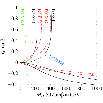
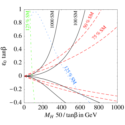
Figure 5: Large $\tan\beta$ effects: $B\to\ell^{+}\bar{\ell}^{-}$ (continuous line), $\Delta M_{B_{s}}$ (dashed red line), $B\to X_{s}\gamma$ (dotted blue line), $B\to X\tau\bar{\nu}_{\tau}$ (dot-dashed green line). Left and right panels correspond to $\epsilon_{2}=\epsilon_{0}$ and $\epsilon_{2}=-\epsilon_{0}$, respectively, in addition to the constraints in eqs. (67).

The most interesting effects generated at the one-loop level are the contributions to dipole operators entering $B\to X_{s}\gamma$. Here we have non-vanishing results both from neutral- and charged-Higgs exchange. Using the effective couplings derived in section 5 we find

$$\delta C_{7\gamma,8G}^{H^{0}}(M^{2}_{W}) = -\frac{(\epsilon_{2}+\epsilon_{3})\tan^{3}\beta}{[1+(\epsilon_{0}+\epsilon_{1})\tan\beta]^{2}[1+(\epsilon_{0}+\epsilon_{1}-\epsilon_{2}-\epsilon_{3})\tan\beta]}~{}\frac{m_{b}^{2}(M^{2}_{W})}{36M_{H}^{2}}~{},$$ (65)

$$\delta C_{7\gamma,8G}^{H^{\pm}}(M^{2}_{W}) = \frac{1}{1+(\epsilon_{0}+\epsilon_{1})\tan\beta}\left[\frac{}{}1+(\epsilon_{0}^{\prime}+\epsilon_{2}^{\prime}+\epsilon_{3}^{\prime})\tan\beta\right.$$ (66)

$$\qquad\qquad\qquad\qquad\left.+\frac{(\epsilon_{2}+\epsilon_{3})(\epsilon_{2}^{\prime}+\epsilon_{3}^{\prime}-\epsilon_{1}^{\prime})\tan^{2}\beta}{1+(\epsilon_{0}+\epsilon_{1}-\epsilon_{2}-\epsilon_{3})\tan\beta}\right]F_{7,8}^{(2)}\left(\frac{m^{2}_{t}}{M_{H}^{2}}\right)~{},\qquad$$

where the functions $F_{7,8}^{(2)}(x)$ can be found in appendix A [in our conventions $C_{7\gamma}^{\rm SM}(M^{2}_{W})<0$]. These results extend those presented in ref. [31]. Even within supersymmetry we find a difference, since the neutral-Higgs-exchange amplitude and the $\epsilon_{i}^{2}\tan^{2}\beta$ terms in the charged-Higgs one (appearing only at the three-loop level in a pure diagrammatic approach) have not been considered in ref. [31]. However, since the neutral-Higgs contribution is numerically small, the effect of these new corrections is limited. Explicit formulæ for the supersymmetric case can be found in appendix A.

If all the $\epsilon_{i}$ are treated as free parameters, the three constraints imposed by $B\to\ell^{+}\ell^{-}$, $\Delta M_{B_{s}}$ and $B\to X_{s}\gamma$ are completely independent. On the other hand, in models where the $\epsilon_{i}$ are calculable these constraints can be combined, leading to interesting bounds on $M_{H}$ and $\tan\beta$. This happens for instance in supersymmetry (see appendix A) where, to a good approximation,

$$\epsilon_{1}=\epsilon_{2}~{},\qquad\epsilon^{\prime}_{0}=-\epsilon_{0}~{},\qquad\epsilon^{\prime}_{1}=-({\hat{\lambda}}_{b}^{2}/{\lambda}_{t}^{2})\epsilon_{1}~{},\qquad\epsilon_{3}=\epsilon_{4}=\epsilon^{\prime}_{2}=\epsilon^{\prime}_{3}=\epsilon^{\prime}_{4}=0~{}.$$ (67)

Motivated by this scenario, in fig. 5 we compare the three constraints employing eqs. (67), supplemented by the additional (simplifying) assumption $\epsilon_{2}=\epsilon_{0}$ or $\epsilon_{2}=-\epsilon_{0}$. We use as variables $\epsilon_{0}\tan\beta$ and $M_{H}/\tan\beta$ because all the effects, except the charged-Higgs amplitude in $B\to X_{s}\gamma$, depend only on these combinations. The $B\to X_{s}\gamma$ bound has been computed assuming $\tan\beta=50$; it can be approximatively rescaled to other $\tan\beta$ values taking into account that, in the limit where the (small) neutral-Higgs exchange amplitude is neglected, the horizontal scale (of this curve only) should be understood as $M_{H}$ instead of $(50/\tan\beta)M_{H}$. For comparison, we have also shown the limit imposed by the tree-level charged-Higgs exchange in $B\to X\tau\bar{\nu}_{\tau}$ [40], which also depends only on $\epsilon_{0}\tan\beta$ and $M_{H}/\tan\beta$ [41]:

$$\frac{{\cal B}(B\to X\tau\bar{\nu}_{\tau})}{{\cal B}(B\to X\tau\bar{\nu}_{\tau})_{\rm SM}}=1-1.2(b_{0}+b_{1})\bigg{(}\frac{m_{\tau}\tan\beta}{m_{H}}\bigg{)}^{2}+\bigg{(}\frac{m_{\tau}m_{b}(b_{0}+b_{1})\tan^{2}\beta}{2m_{H}^{2}}\bigg{)}^{2}~{}.$$ (68)

As can be noted, while the constraints from $B\to X_{s}\gamma$ becomes weaker for large $\epsilon_{0}\tan\beta$ (especially for $\epsilon_{2}=\epsilon_{0}$), the opposite is true for $B_{s}\to\mu\bar{\mu}$ and $\Delta M_{B_{s}}$. As a result, for any value of $\epsilon_{0}\tan\beta$ there is at least one FCNC process setting a bound on $M_{H}$ much stronger than the one imposed by $B\to X\tau\bar{\nu}_{\tau}$.

In the case of the precise measurements of $B\to X\tau\bar{\nu}_{\tau}$ and $B\to X_{s}\gamma$, we have shown in fig. 5 only one curve, corresponding to a maximal enhancement of $25\%$ with respect to the SM value (close to the 90% C.L. limit in both cases). In the case of $\Delta M_{B_{s}}$, where the new contribution leads to a decrease with respect to the SM value, the two curves denotes $50\%$ and $75\%$ of the SM expectation. Due to theoretical uncertainties on the latter, the present 90% C.L. limit is close to the $50\%$ curve. Finally, concerning ${\cal B}(B\to\ell^{+}\ell^{-})$, the two curves correspond to a possible enhancement of two or three orders of magnitude with respect to the SM value (for $\ell=e,\mu$). At the moment the best experimental bound is set by ${\cal B}(B_{s}\to\mu^{+}\mu^{-})$ [16], whose 90% C.L. upper limit is about 900 times the SM value. Clearly, $B\to\ell^{+}\ell^{-}$ decays still have a large discovery potential, for scenarios with large $\tan\beta$, which will be explored in the future both at $e^{+}e^{-}$ $B$-factories and hadron colliders.

7 Some concrete examples

In this section we want to discuss the relation between the MFV operators in our effective theory approach and the flavour-violating interactions in some commonly studied extensions of the SM (partly motivated by the hierarchy problem).

7.1 Supersymmetry

Let us first consider the minimal supersymmetric extension of the SM, with conserved $R$-parity and supersymmetry soft-breaking terms. To understand its structure of flavour-violating couplings, it is convenient to follow the same approach used in previous sections for the SM and the 2HD model. We then take the supersymmetric model as the low-energy effective theory, and we construct all flavour-invariant interactions that contain the spurion fields $Y_{U,D}$. An important difference with the non-supersymmetric case is that we find, beside the ordinary Yukawa couplings, other renormalizable terms with non-trivial flavour structure. Indeed, following the MFV rules, we can write the supersymmetry-breaking squark mass terms and the trilinear couplings as

$${\tilde{m}}_{Q_{L}}^{2} = {\tilde{m}}^{2}\left(a_{1}1{\rm l}+b_{1}Y_{U}Y_{U}^{\dagger}+b_{2}Y_{D}Y_{D}^{\dagger}+b_{3}Y_{D}Y_{D}^{\dagger}Y_{U}Y_{U}^{\dagger}+b_{4}Y_{U}Y_{U}^{\dagger}Y_{D}Y_{D}^{\dagger}\right)~{},$$ (69)

$${\tilde{m}}_{U_{R}}^{2} = {\tilde{m}}^{2}\left(a_{2}1{\rm l}+b_{5}Y_{U}^{\dagger}Y_{U}\right)~{},$$ (70)

$${\tilde{m}}_{D_{R}}^{2} = {\tilde{m}}^{2}\left(a_{3}1{\rm l}+b_{6}Y_{D}^{\dagger}Y_{D}\right)~{},$$ (71)

$$A_{U} = A\left(a_{4}1{\rm l}+b_{7}Y_{D}Y_{D}^{\dagger}\right)Y_{U}~{},$$ (72)

$$A_{D} = A\left(a_{5}1{\rm l}+b_{8}Y_{U}Y_{U}^{\dagger}\right)Y_{D}~{}.$$ (73)

Here $\tilde{m}$ and $A$ set the mass scale of the soft terms, $a_{i}$ and $b_{i}$ are unknown numerical coefficients, and $1{\rm l}$ is the $3\times 3$ identity matrix. In obtaining eqs. (69)–(73), we have kept all independent flavour structures proportional to third-generation Yukawa couplings (similarly to the $\epsilon_{i}$ of sect. 5, possible polynomials of $({\lambda}_{u,d})_{33}$ can be reabsorbed in the definition of $a_{i}$ and $b_{i}$) but we have neglected contributions quadratic in the Yukawas of the first two families. When $\tan\beta$ is not too large and the bottom Yukawa coupling is small, the terms quadratic in $Y_{D}$ can be dropped from eqs. (69)–(73).

The assumption of universality of soft masses and proportionality of trilinear terms corresponds to setting all $b_{i}$ coefficients to zero. This hypothesis is not renormalization-group invariant, and it is usually taken to hold at a high-energy scale $\Lambda$, whose value can be inferred by knowledge of the specific mechanism of supersymmetry breaking. Then the coefficients $b_{i}$ are generated by renormalization-group evolution, and their typical size is $(1/4\pi)^{2}\ln\Lambda^{2}/{\tilde{m}}^{2}$. For sufficiently large values of $\Lambda$, the effect can be significant. The $b_{i}$ coefficients can also be generated by integrating out heavy states at the cut-off scale $\Lambda$ (assuming that the high-energy dynamics satisfies MFV). This mechanism can also lead to sizable effects, since the new contributions to $b_{i}$ are not suppressed by powers of the scale $\Lambda$. This high-energy sensitivity of the flavour structure in the soft terms [42] makes the MFV assumption in supersymmetry rather tottery. In particular, in supergravity where $\Lambda$ has to be identified with a scale close to the Planck mass, MFV in the soft terms requires that all dynamics up to the gravitational scale must satisfy MFV. This is quite possible but, from the low-energy point of view, it appears as a strong assumption. The situation improves in models with gauge-mediated supersymmetry breaking [43], since the scale $\Lambda$ is identified with the mass of hypothetical messenger particles. This mass scale is arbitrary, and it can be low enough to reduce the region of high-energy sensitivity. In anomaly mediation [44] the problem is bypassed, since the soft terms are driven towards universality by renormalization-group evolution, irrespectively of their high-energy values.

Using the soft terms in eqs. (69)–(73), the physical squark $6\times 6$ mass matrices, after electroweak breaking, are given by

$${\tilde{M}}_{U}^{2}=\pmatrix{{\tilde{m}}_{Q_{L}}^{2}+Y_{U}Y_{U}^{\dagger}v_{U}^{2}+\left(\frac{1}{2}-\frac{2}{3}\sin^{2}\theta_{\rm W}\right)M_{Z}^{2}\cos 2\beta&\left(A_{U}-\mu Y_{U}\cot\beta\right)v_{U}\cr\left(A_{U}-\mu Y_{U}\cot\beta\right)^{\dagger}v_{U}&\!\!\!\!\!\!{\tilde{m}}_{U_{R}}^{2}+Y_{U}^{\dagger}Y_{U}v_{U}^{2}+\frac{2}{3}\sin^{2}\theta_{\rm W}M_{Z}^{2}\cos 2\beta}~{},$$ (74)

$${\tilde{M}}_{D}^{2}=\pmatrix{{\tilde{m}}_{Q_{L}}^{2}+Y_{D}Y_{D}^{\dagger}v_{D}^{2}-\left(\frac{1}{2}-\frac{1}{3}\sin^{2}\theta_{\rm W}\right)M_{Z}^{2}\cos 2\beta&\left(A_{D}-\mu Y_{D}\tan\beta\right)v_{D}\cr\left(A_{D}-\mu Y_{D}\tan\beta\right)^{\dagger}v_{D}&\!\!\!\!\!\!{\tilde{m}}_{D_{R}}^{2}+Y_{D}^{\dagger}Y_{D}v_{D}^{2}-\frac{1}{3}\sin^{2}\theta_{\rm W}M_{Z}^{2}\cos 2\beta}~{}.$$ (75)

Here $\mu$ is the higgsino mass parameter and $v_{U,D}$ the two Higgs vacuum expectation values ($\tan\beta=v_{U}/v_{D}$).

The squark mass matrices are diagonalized by the unitary transformations $T_{U,D}{\tilde{M}}_{U,D}^{2}T_{U,D}^{\dagger}$. When all $b_{i}$ coefficients in eqs. (69)–(73) are negligible, in the basis of eq. (5), the rotation matrices are given by

$$T_{U}=\pmatrix{C_{U}V&S_{U}\cr-S_{U}V&C_{U}}~{},~{}~{}~{}~{}T_{D}=\pmatrix{C_{D}&S_{D}\cr-S_{D}&C_{D}}~{},$$ (76)

$$C_{U,D}={\rm diag}\left(\cos\theta_{U_{i},D_{i}}\right)~{},~{}~{}~{}~{}S_{U,D}={\rm diag}\left(\sin\theta_{U_{i},D_{i}}\right)~{},$$ (77)

$$\tan 2\theta_{U_{i}}=\frac{2(Aa_{4}-\mu\cot\beta)m_{u_{i}}}{(a_{1}-a_{2}){\tilde{m}}^{2}+\left(\frac{1}{2}-\frac{4}{3}\sin^{2}\theta_{\rm W}\right)M_{Z}^{2}\cos 2\beta}~{},$$ (78)

$$\tan 2\theta_{D_{i}}=\frac{2(Aa_{5}-\mu\tan\beta)m_{d_{i}}}{(a_{1}-a_{3}){\tilde{m}}^{2}-\left(\frac{1}{2}-\frac{2}{3}\sin^{2}\theta_{\rm W}\right)M_{Z}^{2}\cos 2\beta}~{}.$$ (79)

Here $m_{u_{i}}$ and $m_{d_{i}}$ are the corresponding tree-level quark masses. In this case, the rotations in flavour space of squarks and quarks are the same, therefore tree-level flavour-changing transitions occur only in the charged current coupled to charginos, with angles equal to those of $V$. Notice that the left-right squark mixing does not modify the flavour structure, although it complicates the expressions of the diagonalization matrices.

When non-vanishing $b_{i}$ coefficients are included in the soft terms, the diagonalization of the mass matrices in eqs. (74) and (75) is, in general, more involved. However, if $\tan\beta$ is not large and the bottom Yukawa coupling can be neglected, we can easily express the squark rotations as

$$T_{U}=\pmatrix{C_{U}^{\prime}V&S_{U}^{\prime}\cr-S_{U}^{\prime}V&C_{U}^{\prime}},~{}~{}~{}~{}T_{D}=\pmatrix{V&0\cr 0&1{\rm l}}~{},$$ (80)

$$C_{U}^{\prime}={\rm diag}\left(\cos\theta_{U_{i}}^{\prime}\right)~{},~{}~{}~{}~{}S_{U}^{\prime}={\rm diag}\left(\sin\theta_{U_{i}}^{\prime}\right)~{},$$ (81)

$$\tan 2\theta_{U_{i}}^{\prime}=\frac{2(Aa_{4}-\mu\cot\beta)m_{u_{i}}}{(a_{1}-a_{2}){\tilde{m}}^{2}+(b_{1}-b_{5}){\tilde{m}}^{2}m_{u_{i}}^{2}/v_{U}^{2}+\left(\frac{1}{2}-\frac{4}{3}\sin^{2}\theta_{\rm W}\right)M_{Z}^{2}\cos 2\beta}~{}.$$ (82)

In this case, the rotation in flavour space of down-type quarks and left down squarks is different, and tree-level flavour-changing transitions occur in neutral currents coupled to gluinos and neutralinos, with angles equal to those of $V$.

The next step is to integrate out the supersymmetric particles at one loop. In the limit where the soft mass parameters are sufficiently larger than the Higgs vacuum expectation values, this step should be performed before considering the ${\rm SU}(2)_{L}$ breaking. As a result, one obtains a series of higher-dimensional ${\rm SU}(2)_{L}$-invariant operators, whose leading (dimension-six) terms are those discussed in the previous sections. Following this approach, the coefficients of the MFV operators are computable in terms of supersymmetric soft-breaking parameters. In principle, one could be worried by the fact that the assumption ${\tilde{m}}\gg v_{U,D}$ is not necessarily a good approximation; however, it should be noticed that the leading ${\rm SU}(2)_{L}$-breaking effects associated with the third family do not spoil the structure of the operator basis discussed in the previous sections, since they can be reabsorbed by appropriate coefficient functions. Notice also that the integration of the supersymmetric degrees of freedom leads to a modification of the renormalizable operators and, in particular, of the Yukawa interaction. As a result, in an effective field theory with supersymmetric degrees of freedom, the relations between $Y_{U,D}$ and the physical quark masses and CKM angles are potentially modified. Since no large logarithms are involved, this effect is usually small, with the exception of the large $\tan\beta$ case, discussed in detail in sect. 5 and 6.

We stress that the MFV hypothesis does not imply that the physical squark masses are all equal, but the form of the mass splittings is tightly constrained, see eqs. (74) and (75). One could think of a departure from MFV, by assuming that the squark masses of the third generation are different from those of the other two, as motivated by the requirement of a reduced fine tuning [45]. In this case, some SU(3) factors of the flavour group are broken into SU(2). Then new flavour spurions with non-vanishing background values along the third-generation component, in a basis in which neither $Y_{U}$ nor $Y_{D}$ is necessarily diagonal, should be added in the effective-theory analysis. The flavour effects in this scenario have been studied in ref. [46].

7.2 Technicolour and extra dimensions

In technicolour theories, the generation of fermion masses leads to a chronic problem with flavour violation. In the absence of a completely successful solution, the MFV effective-theory approach seems well suited to compare experimental results with model-building attempts. Indeed the approach we are following in this paper is closely related to the one pioneered by Chivukula and Georgi in the framework of technicolour [1].

Models with a low quantum-gravity scale, based on extra-dimensional scenarios, are also a natural arena for the MFV effective theory [47], since the underlying theory is unknown and its low-energy limit becomes strongly-interacting at a scale which is expected to be not much larger than the weak scale. In some cases the effects in extra-dimensional models are nevertheless computable. Tree level exchange of Kaluza-Klein excitations of SM fermions [48], of the SM vector bosons, of the Higgs, and of the graviton do not give rise to significant flavour-violating effects. For instance, it is easy to realize that the exchange of the Higgs excitations can sizeably affect only four-fermion operators involving the top quark, which are not relevant for our discussion.

As noticed in [49], large tree-level flavour-violating effects mediated by Kaluza-Klein excitations of gauge bosons appear in models in which fermions are confined on different locations within a thick brane where gauge forces can propagate. Such models have been proposed to give a geometrical justification of the observed hierarchy of quarks and lepton masses [50]. The dangerous flavour-violating interactions are caused by the non-trivial profile of the excited gauge modes along the new dimensions, which leads to flavour-dependent couplings with the fermions situated at different positions in the extra coordinates. These models violate the MFV hypothesis, and indeed the limit on the mass of the first Kaluza-Klein gauge-boson mode is extremely stringent, of the order of 5000 TeV [49].

At first sight it appears quite problematic to impose MFV to a quantum-gravity theory with fundamental scale at the TeV. This is because we cannot play with a very high-energy scale to suppress unwanted flavour-violating operators. The most realistic attempt so far proposed makes use of the extra dimensions to solve the problem. It is based on locality (flavour-violating interactions are confined on one brane) and geometry (we live on a second brane, distant from the first one, and therefore we observe very suppressed flavour-violating effective interactions) [51]. In this scheme, to generate Yukawa couplings, it is necessary to have bulk fields, charged under the flavour group, which mediate the information of flavour symmetry breaking between the two branes. These bulk fields can also generate new flavour violating effects, which respect the hypothesis of MFV by construction. In the context of models with a warped extra dimension [52], the emergence of bulk fields with flavour charge from the request of MFV has a nice interpretation through the AdS/CFT correspondence. Indeed, if we impose a global flavour symmetry on the 4-dimensional CFT, we find in the AdS picture, 5-dimensional bulk gauge fields for the flavour group and also Yukawa couplings promoted to scalar bulk fields [53]. Using this language, one can also understand the relation between the usual flavour suppressions due to operators with a very high-energy effective scale and suppression due to extra-dimensional locality, since the distance along the 5th coordinate is mapped into the renormalization energy scale of the 4-dimensional CFT.

Vector bosons of the SU(3)⁵ flavour symmetry in the bulk generate, at low energies, various effective operators. Their tree-level exchange, in the case of a 5-dimensional theory, is particularly interesting since the coefficients of these operators are finite and computable. In the exact flavour limit (with the Yukawa couplings set to zero), the strongest constraint comes from the flavour-conserving operator $\frac{1}{2}(\bar{L}\gamma_{\mu}\tau^{a}L)^{2}$, whose coefficient is limited by present data on muon decay to have an effective scale larger than $\Lambda\,\raise 1.29167pt\hbox{$>$\kern-7.5pt\lower 4.30554pt\hbox{$\sim$}}\,5\,{\rm TeV}$ at $99\%$ CL [54]. Once we consider insertions of the scalar bulk fields $Y_{U,D,E}$ (whose background values determine the Yukawa couplings), then specific MFV operators are generated: the $\Delta F=2$ operator ${\cal O}_{0}$ and some combinations of the $\Delta F=1$ four-quark operators. Operators giving rise to $b\to s\gamma$ are generated at one-loop level.

8 Conclusions

The starting point of our analysis has been a general definition of MFV, in an effective-theory approach. The basic assumption of MFV is that the only source of SU(3)⁵ flavour breaking is given by the background value of scalar fields $Y$ which have the same transformation properties under the flavour group as the ordinary Yukawa couplings. The interaction Lagrangian of the MFV effective theory valid below the energy scale $\Lambda$ is constructed, in terms of the SM fields and the spurions $Y$, by assuming flavour and CP invariance.

We believe that this definition of MFV leads to a realistic description of the minimal effects in flavour physics almost necessarily present in any extension of the Standard Model with non-trivial dynamics at the scale $\Lambda$. It would be unrealistic to impose the more restrictive assumption that all higher-dimensional effective operators are flavour invariant and contain only SM fields (and not $Y$), since SU(3)⁵ flavour is not a symmetry of the SM. Our definition of MFV is consistent with the existence of Yukawa couplings in the low-energy theory. Also, the more restrictive assumption indeed does not hold in known extensions of the SM, like supersymmetry. On the other hand, for an effective theory derived from supersymmetry, our definition coincides with the usual requirements of supersymmetric MFV: $R$-parity conservation, flavour-universal soft scalar masses, and trilinear terms proportional to the corresponding Yukawa couplings. In the case of supersymmetry, the effective-theory language employed here is just a useful bookkeeping device, but its use is especially suited for theories in which the dynamics at the scale $\Lambda$ is not fully known or perturbatively calculable, as in the case of technicolour or theories with low-scale quantum gravity.

If the effective theory is built from the SM with a single Higgs doublet, we have found that all new (non-negligible) flavour-violating effects involve a single flavour structure $\lambda_{\rm FC}$. We have then presented a general classification of dimension-6 effective operators containing $\lambda_{\rm FC}$ and we have collected in table 1 the present bounds on their coefficients $1/\Lambda^{2}$ (assuming the presence of a single operator at a time).

The most stringent bound, coming from $B\to X_{s}\gamma$, is on the coefficient of the magnetic operator ${\cal O}_{F_{1}}$, whose scale $\Lambda$ is constrained to be larger than 12.4 TeV (for constructive interference with the SM amplitude) or 9.3 TeV (for destructive interference) at 99% CL. A narrow range of $\Lambda$ around 3 TeV is allowed by the data (see fig. 2), corresponding to a decay amplitude equal in size to the SM value but opposite in sign. Leaving aside this fine-tuned case (or the case in which the contribution from the chromomagnetic operator ${\cal O}_{G_{1}}$ compensates the effect from ${\cal O}_{F_{1}}$), this result shows that $B\to X_{s}\gamma$ poses a highly non-trivial bound on $\Lambda$, especially for theories in which this cut-off scale has to be identified with the electroweak scale, as in many theories motivated by the hierarchy problem.

The second best bound after $B\to X_{s}\gamma$ is obtained, at present, by the CP-violating parameter $\epsilon_{K}$, which constrains the scale of the $\Delta F=2$ effective operator ${\cal O}_{0}$ to be larger than 5.0 or 6.4 TeV (for constructive or destructive interference with the SM amplitude). This bound is determined within a global fit of the CKM unitarity triangle which, to a large extent, is not affected by the existence of the new operators. In particular, time-dependent CP-violating asymmetries in the $B$ system are not by themselves, or when compared to tree-level processes, good probes of MFV models. If MFV is realized, deviations from SM expectations can be detected only by measuring the full strenght of FCNC transitions.

An important feature of the existence of a single flavour-violating structure $\lambda_{\rm FC}$ is the possibly of relating predictions for various FCNC processes both in the $K$ and in the $B$ system. In table 3 we show limits on some FCNC decays (stronger than the present experimental bounds) derived from the MFV assumption and from data on other processes. If future experimental searches give evidence for violation of any of the bounds in table 3, not only will we discover new physics, but we will also learn that its dynamics at the scale $\Lambda$ has a flavour structure beyond MFV. This will have important consequences for model building.

Moreover, the MFV interplay between various processes in $K$ and $B$ physics allows an interesting comparison between different experimental searches, as illustrated in figs. 3 and 4. For instance, future experimental investigation of the process $B\to X_{s}\ell^{+}\ell^{-}$ is expected to improve the sensitivity on the coefficients of the operators ${\cal O}_{\ell_{1}\ldots\ell_{3}}$, and ${\cal O}_{H_{1},H_{2}}$. These new results (in case of a negative search) will strengthen the MFV limits presented in table 3. Because of its theoretical cleanliness, the process $K_{L}\to\pi^{0}\nu\bar{\nu}$ has an even bigger potential for setting bounds on $\Lambda$, in the long-term future.

A significant difference in the analysis emerges if we construct the effective theory starting from the SM with an enlarged Higgs sector containing two scalar doublets. Since the bottom-quark Yukawa coupling can now be non-negligible and even of order unity (when $\tan\beta$ is large and of order $m_{t}/m_{b}$), then it is possible to construct flavour-violating operators with a flavour structure different than $\lambda_{\rm FC}$. We have presented a general procedure to include all new flavour-violating effects, when $\tan\beta$ is large. These effects can be parametrized by the eight (PQ-violating) $\epsilon$ coefficients defined in eqs. (42) and  (41), which modify the flavour-violating neutral and charged currents coupled to the Higgs bosons as given in eqs. (50) and (52). New significant contributions appear in several $B$ processes, with the most interesting effects in $B\to\ell^{+}\ell^{-}$ and $B\to X_{s}\gamma$. These two processes play a complementary rôle in constraining the charged Higgs mass, in the large $\tan\beta$ limit, see fig. 5. Indeed, $B\to\ell^{+}\ell^{-}$ is more constraining at large values of $|\epsilon|\tan\beta$ while, for small $|\epsilon|\tan\beta$, $B\to X_{s}\gamma$ becomes more effective.

The two-Higgs doublet analysis can also be used in supersymmetric models with large $\tan\beta$. In this case, the $\epsilon$ parameters are determined by a one-loop diagram involving supersymmetric particles. Our procedure gives the exact result to all orders in $\epsilon\tan\beta$, in the ${\rm SU}(2)_{L}$-symmetric limit, therefore it effectively resums the leading terms at any loop level. With this technique, we have found two-loop contributions to $B\to X_{s}\gamma$ mediated by neutral Higgs bosons and three-loop contributions mediated by the charged Higgs boson, which were not known but that can be non-negligible in the large $\tan\beta$ limit.

Appendix

Appendix A Higgs-mediated $\tan\beta$-enhanced contributions to $B\to X_{s}\gamma$ in supersymmetry

In this appendix we collect the formulæ necessary to compute the $\epsilon_{i}\tan\beta$ corrections to the heavy-Higgs (charged and neutral) $B\to X_{s}\gamma$ amplitude in supersymmetry. As is well known, these corrections do not vanish in the limit of heavy sparticles: using the general results of section 5, we can re-sum them to all orders in the ${\rm SU}(2)_{L}$-symmetric limit ($v^{2}\ll{\tilde{m}}^{2}$).

The dimension-four non-holomorphic terms generated at one loop by gluino and Higgsino diagrams [28], computed in the ${\rm SU}(2)_{L}$-symmetric limit, can be written as

$$\mathscr{L}_{\epsilon Y}^{\rm SUSY} = -\frac{2\alpha_{\rm s}\mu}{3\pi m_{\tilde{g}}}\left[H_{2}\left(\frac{m_{{\tilde{q}}_{L}}^{2}}{m_{\tilde{g}}^{2}},\frac{m_{{\tilde{d}}_{R}}^{2}}{m_{\tilde{g}}^{2}}\right){\bar{Q}}_{L}{Y}_{D}D_{R}(H_{U})^{c}-H_{2}\left(\frac{m_{{\tilde{q}}_{L}}^{2}}{m_{\tilde{g}}^{2}},\frac{m_{{\tilde{u}}_{R}}^{2}}{m_{\tilde{g}}^{2}}\right){\bar{Q}}_{L}{Y}_{U}U_{R}(H_{D})^{c}\right]$$ (83)

$$-\frac{A}{16\pi^{2}\mu}H_{2}\left(\frac{m_{{\tilde{q}}_{L}}^{2}}{\mu^{2}},\frac{m_{{\tilde{u}}_{R}}^{2}}{\mu^{2}}\right){\bar{Q}}_{L}{Y}_{U}{Y}_{U}^{\dagger}{Y}_{D}D_{R}(H_{U})^{c}$$

$$+\frac{A}{16\pi^{2}\mu}H_{2}\left(\frac{m_{{\tilde{q}}_{L}}^{2}}{\mu^{2}},\frac{m_{{\tilde{d}}_{R}}^{2}}{\mu^{2}}\right){\bar{Q}}_{L}{Y}_{U}{Y}_{D}{Y}_{D}^{\dagger}U_{R}(H_{D})^{c}~{}+{\rm h.c.},$$

where

$$H_{2}(x,y)=\frac{x\ln\,x}{(1-x)(x-y)}+\frac{y\ln\,y}{(1-y)(y-x)}$$ (84)

and, as usual, $\mu$ denotes the supersymmetric Higgs mass term and $A$ the three-linear soft-breaking term. Comparing $\mathscr{L}_{\epsilon Y}^{\rm SUSY}$ with the general expression in eqs. (41)–(42), it follows

$$\epsilon_{0}=-\frac{2\alpha_{\rm s}\mu}{3\pi m_{\tilde{g}}}H_{2}\left(\frac{m_{{\tilde{q}}_{L}}^{2}}{m_{\tilde{g}}^{2}},\frac{m_{{\tilde{d}}_{R}}^{2}}{m_{\tilde{g}}^{2}}\right)~{},\qquad\epsilon_{0}^{\prime}=\frac{2\alpha_{\rm s}\mu}{3\pi m_{\tilde{g}}}H_{2}\left(\frac{m_{{\tilde{q}}_{L}}^{2}}{m_{\tilde{g}}^{2}},\frac{m_{{\tilde{u}}_{R}}^{2}}{m_{\tilde{g}}^{2}}\right)~{},$$

$$\epsilon_{2}=-\frac{A\lambda_{t}^{2}}{16\pi^{2}\mu}H_{2}\left(\frac{m_{{\tilde{q}}_{L}}^{2}}{\mu^{2}},\frac{m_{{\tilde{u}}_{R}}^{2}}{\mu^{2}}\right)~{},\qquad\epsilon_{1}=\epsilon_{2}~{},$$

$$\epsilon_{1}^{\prime}=\frac{A{\hat{\lambda}}_{b}^{2}}{16\pi^{2}\mu}H_{2}\left(\frac{m_{{\tilde{q}}_{L}}^{2}}{\mu^{2}},\frac{m_{{\tilde{d}}_{R}}^{2}}{\mu^{2}}\right)~{},\qquad\epsilon_{3}=\epsilon_{4}=\epsilon^{\prime}_{2}=\epsilon^{\prime}_{3}=\epsilon^{\prime}_{4}=0~{},$$ (85)

where

$${\hat{\lambda}}_{b}=\frac{1}{\cos\beta}\left[2\sqrt{2}G_{F}\right]^{1/2}\frac{m_{b}}{[1+(\epsilon_{0}+\epsilon_{2})\tan\beta]}~{}.$$ (86)

In the limit where right-handed up and down squarks are degenerate, only two of these terms are independent and we recover the relations (67).

Figure 6: Deviations of ${\cal B}(B\to X_{s}\gamma)$ with respect to the SM value due to (supersymmetric) heavy-Higgs exchanges. The two full (red) lines correspond to the full result in eq. (87), for $\epsilon_{2}=\pm\epsilon_{0}$. The dashed lines do not contain the new (higher-order) contributions identified in this paper (see text). All curves have been obtained for $M_{H}=250$ GeV, $\tan\beta=50$ and $\epsilon^{\prime}_{0}=-\epsilon_{0}$.

The supersymmetric $\epsilon_{i}$ induce four types of $\tan\beta$-enhanced corrections, which all affect the $B\to X_{s}\gamma$ amplitude: i) the modified relation between $m_{b}$ and the $b$-quark Yukawa coupling; ii) the modified relation between $m_{t}$ and the $\bar{t}_{R}d_{L}H^{+}$ vertex; iii) the FCNC ${\bar{s}}_{L}b_{R}H^{0}_{D}$ coupling; iv) the modification of $V_{ts}$. All these effects are taken into account to all orders when using the effective Lagrangians (50) and (52) to compute the Higgs couplings. Computing both charged- and neutral-Higgs exchange amplitudes, at one loop, with these effective vertices, we find

$$C_{7\gamma,8G}^{H}(\mu_{\scriptscriptstyle W}) = \frac{1}{1+(\epsilon_{0}+\epsilon_{2})\tan\beta}\left[1+\epsilon^{\prime}_{0}\tan\beta-\frac{\epsilon_{2}\epsilon_{1}^{\prime}\tan^{2}\beta}{1+\epsilon_{0}\tan\beta}\right]F_{7,8}^{(2)}\left(\frac{m^{2}_{t}(\mu_{\scriptscriptstyle W})}{M_{H}^{2}}\right)$$ (87)

$$- \frac{\epsilon_{2}\tan^{3}\beta}{[1+(\epsilon_{0}+\epsilon_{2})\tan\beta]^{2}[1+\epsilon_{0}\tan\beta]}~{}\frac{m_{b}^{2}(\mu_{\scriptscriptstyle W})}{36M_{H}^{2}}~{},\qquad$$

where

$$F_{7}^{(2)}(y) = \frac{y(3-5y)}{12(y-1)^{2}}+\frac{y(3y-2)}{6(y-1)^{3}}\ln y~{},$$ (88)

$$F_{8}^{(2)}(y) = \frac{y(3-y)}{4(y-1)^{2}}-\frac{y}{2(y-1)^{3}}\ln y~{}.$$ (89)

The contributions which have not been considered before in the literature, namely the $\tan^{2}\beta$ term in the charged-Higgs part and the full neutral-Higgs amplitude, are numerically rather suppressed, except for large $\epsilon\tan\beta$. As illustrated in figure 6, these contributions are essentially negligible, independently of $\epsilon_{0}\tan\beta$, if $\epsilon_{2}\approx\epsilon_{0}$. On the other hand, sizable effects arise if $\epsilon_{2}\approx-\epsilon_{0}$. In particular, for $\epsilon^{\prime}_{0}\tan\beta\approx-\epsilon_{0}\tan\beta\approx-1$, where the leading term vanishes, these higher-order contributions could even become the dominant non-standard effect.

Appendix B The ${\cal Q}_{i}$ basis

Quark-lepton currents:

$${\cal Q}_{\nu\bar{\nu}} = \bar{d}_{i}\gamma_{\mu}(1-\gamma_{5})d_{j}~{}\bar{\nu}\gamma_{\mu}(1-\gamma_{5})\nu$$

$${\cal Q}_{10A} = \bar{d}_{i}\gamma_{\mu}(1-\gamma_{5})d_{j}~{}\bar{\ell}\gamma_{\mu}\gamma_{5}\ell$$

$${\cal Q}_{9V} = \bar{d}_{i}\gamma_{\mu}(1-\gamma_{5})d_{j}~{}\bar{\ell}\gamma_{\mu}\ell$$ (90)

Non-leptonic electroweak operators:

$${\cal Q}_{7} = \bar{d}^{\alpha}_{i}\gamma_{\mu}(1-\gamma_{5})d^{\alpha}_{j}~{}\sum_{q}e_{q}\bar{q}^{\beta}\gamma_{\mu}(1+\gamma_{5})q^{\beta}$$

$${\cal Q}_{8} = \bar{d}^{\alpha}_{i}\gamma_{\mu}(1-\gamma_{5})d^{\beta}_{j}~{}\sum_{q}e_{q}\bar{q}^{\beta}\gamma_{\mu}(1+\gamma_{5})q^{\alpha}$$

$${\cal Q}_{9} = \bar{d}^{\alpha}_{i}\gamma_{\mu}(1-\gamma_{5})d^{\alpha}_{j}~{}\sum_{q}e_{q}\bar{q}^{\beta}\gamma_{\mu}(1-\gamma_{5})q^{\beta}$$

$${\cal Q}_{10} = \bar{d}^{\alpha}_{i}\gamma_{\mu}(1-\gamma_{5})d^{\beta}_{j}~{}\sum_{q}e_{q}\bar{q}^{\beta}\gamma_{\mu}(1-\gamma_{5})q^{\alpha}$$ (91)

Dipole operators:

$${\cal Q}_{7\gamma} = \frac{1}{g^{2}}m_{d_{i}}\bar{d}_{i}(1-\gamma_{5})\sigma_{\mu\nu}d_{j}(eF_{\mu\nu})$$

$${\cal Q}_{8G} = \frac{1}{g^{2}}m_{d_{i}}\bar{d}_{i}(1-\gamma_{5})\sigma_{\mu\nu}T^{a}d_{j}(g_{s}G^{a}_{\mu\nu})$$ (92)

References

• [1] R. S. Chivukula and H. Georgi, Phys. Lett. B 188 (1987) 99.
• [2] R. D. Peccei and H. R. Quinn, Phys. Rev. D 16 (1977) 1791.
• [3] G. Buchalla, A.J. Buras and M.E. Lautenbacher, Rev. Mod. Phys. 68 (1996) 1125 [hep-ph/9512380].
• [4] B. Aubert et al. [Babar Collab.], hep-ex/0203007; K. Abe et al. [Belle Collab.], hep-ex/0207098
• [5] M. Ciuchini et al., JHEP 0107 (2001) 013 [hep-ph/0012308].
• [6] A. Ali and D. London, Eur. Phys. J. C 9 (1999) 687 [hep-ph/9903535]; A. J. Buras et al., Phys. Lett. B 500 (2001) 161 [hep-ph/0007085].
• [7] A. J. Buras and R. Fleischer, Phys. Rev. D 64 (2001) 115010 [hep-ph/0104238]; S. Laplace, Z. Ligeti, Y. Nir and G. Perez, Phys. Rev. D 65 (2002) 094040 [hep-ph/0202010].
• [8] A. J. Buras, M. E. Lautenbacher and G. Ostermaier, Phys. Rev. D 50 (1994) 3433 [hep-ph/9403384].
• [9] S. Chen et al. [CLEO Collab.], hep-ex/0108032.
• [10] K. Abe et al. [Belle Collab.], Phys. Lett. B 511 (2001) 151 [hep-ex/0103042].
• [11] B. Aubert et al [Babar Collab.], hep-ex/0207076.
• [12] P. Gambino and M. Misiak, Nucl. Phys. B 611 (2001) 338 [hep-ph/0104034].
• [13] K. G. Chetyrkin, M. Misiak and M. Munz, Phys. Lett. B 400 (1997) 206; ibid. 425 (1998) 414(E) [hep-ph/9612313].
• [14] M. Ciuchini, G. Degrassi, P. Gambino and G. F. Giudice, Nucl. Phys. B 534 (1998) 3 [hep-ph/9806308].
• [15] G. D’Ambrosio and G. Isidori, Int. J. Mod. Phys. A 13 (1998) 1 [hep-ph/9611284]; G. Colangelo, G. Isidori and J. Portoles, Phys. Lett. B 470 (1999) 134 [hep-ph/9908415].
• [16] Particle data group, Eur. Phys. J. C 15 (2000) 1 and 2001 off-year partial update for the 2002 edition, available at the internet address pdg.lbl.gov.
• [17] B. Aubert et al.  [BABAR Collab.],   hep-ex/0207083.
• [18] G. Buchalla and A. J. Buras, Nucl. Phys. B 548 (1999) 309 [hep-ph/9901288].
• [19] S. Adler et al.  [E787 Collab.],  hep-ex/0111091; S. Adler et al. [E787 Collab.], Phys. Rev. Lett. 84 (2000) 3768 [hep-ex/0002015]; ibid. 79 (1997) 2204 [hep-ex/9708031];
• [20] S. Bergmann and G. Perez, Phys. Rev. D 64 (2001) 115009 [hep-ph/0103299].
• [21] D. Ambrose et al. [E871 Collab.], Phys. Rev. Lett. 84 (2000) 1389.
• [22] G. D’Ambrosio, G. Isidori and J. Portolés, Phys. Lett. B 423 (1998) 385 [hep-ph/9708326]; G. Dumm and A. Pich, Phys. Rev. Lett. 80 (1998) 4633 [hep-ph/980129].
• [23] A. Ali, G. F. Giudice and T. Mannel, Z. Phys. C 67 (1995) 417 [hep-ph/9408213].
• [24] K. Abe et al. [Belle Collab.], Phys. Rev. Lett. 88 (2002) 021801 [hep-ex/0109026]; K. Abe et al. [Belle Collab.], hep-ex/0107072.
• [25] B. Aubert et al. [Babar Collab.], arXiv:hep-ex/0207082.
• [26] A. Ali, E. Lunghi, C. Greub and G. Hiller, hep-ph/0112300.
• [27] A. Ali, P. Ball, L. T. Handoko and G. Hiller, Phys. Rev. D 61 (2000) 074024 [hep-ph/9910221].
• [28] L. J. Hall, R. Rattazzi and U. Sarid, Phys. Rev. D 50 (1994) 7048 [hep-ph/9306309].
• [29] T. Blazek, S. Raby and S. Pokorski, Phys. Rev. D 52 (1995) 4151 [hep-ph/9504364].
• [30] M. Carena, D. Garcia, U. Nierste and C. E. Wagner, Nucl. Phys. B 577 (2000) 88 [hep-ph/9912516].
• [31] G. Degrassi, P. Gambino and G. F. Giudice, JHEP 0012 (2000) 009 [hep-ph/0009337]; M. Carena, D. Garcia, U. Nierste and C. E. Wagner, Phys. Lett. B 499 (2001) 141 [hep-ph/0010003].
• [32] C. Hamzaoui, M. Pospelov and M. Toharia; Phys. Rev. D 59 (1999) 095005 [hep-ph/9807350]. K. S. Babu and C. Kolda, Phys. Rev. Lett. 84 (2000) 228 [hep-ph/9909476].
• [33] G. Isidori and A. Retico, JHEP 0111 (2001) 001 [hep-ph/0110121].
• [34] C. Bobeth, T. Ewerth, F. Kruger and J. Urban, Phys. Rev. D 64 (2001) 074014 [hep-ph/0104284].
• [35] Q. S. Yan, C. S. Huang, W. Liao and S. H. Zhu, Phys. Rev. D 62, 094023 (2000) [hep-ph/0004262]; D. A. Demir, K. A. Olive and M. B. Voloshin, hep-ph/0204119.
• [36] P. H. Chankowski and L. Slawianowska, Phys. Rev. D 63 (2001) 054012 [hep-ph/0008046]. C. S. Huang, W. Liao, Q. S. Yan and S. H. Zhu, Phys. Rev. D 63 (2001) 114021, ibid. 64 (2001) 059902 (E) [hep-ph/0006250]; A. Dedes, H. K. Dreiner and U. Nierste, Phys. Rev. Lett. 87 (2001) 251804 [hep-ph/0108037].
• [37] See e.g. A. F. Falk, Y. Grossman, Z. Ligeti and A. A. Petrov, Phys. Rev. D 65 (2002) 054034 [hep-ph/0110317] and references there in.
• [38] G. Burdman, E. Golowich, J. Hewett and S. Pakvasa, hep-ph/0112235.
• [39] A. J. Buras, P. H. Chankowski, J. Rosiek and L. Slawianowska, Nucl. Phys. B 619 (2001) 434 [hep-ph/0107048].
• [40] R. Barate et al. [ALEPH Collab.] Eur. Phys. J. C 19 (2001) 213 [hep-ex/0010022].
• [41] J. Kalinowski, Phys. Lett. B 245 (1990) 201; Y. Grossman and Z. Ligeti, Phys. Lett. B 332 (1994) 373 [hep-ph/9403376].
• [42] L. J. Hall, V. A. Kostelecky and S. Raby, Nucl. Phys. B 267 (1986) 415.
• [43] M. Dine and A. E. Nelson, Phys. Rev. D 48 (1993) 1277 [hep-ph/9303230]; M. Dine, A. E. Nelson and Y. Shirman, Phys. Rev. D 51 (1995) 1362 [hep-ph/9408384]; G. F. Giudice and R. Rattazzi, Phys. Rep. 322 (1999) 419 [hep-ph/9801271].
• [44] L. Randall and R. Sundrum, Nucl. Phys. B 557 (1999) 79 [hep-th/9810155]; G. F. Giudice, M. A. Luty, H. Murayama and R. Rattazzi, JHEP 9812 (1998) 027 [hep-ph/9810442].
• [45] S. Dimopoulos and G. F. Giudice, Phys. Lett. B 357 (1995) 573 [hep-ph/9507282]; A. G. Cohen, D. B. Kaplan and A. E. Nelson, Phys. Lett. B 388 (1996) 588 [hep-ph/9607394].
• [46] A. G. Cohen, D. B. Kaplan, F. Lepeintre and A. E. Nelson, Phys. Rev. Lett. 78 (1997) 2300 [hep-ph/9610252].
• [47] See e.g. Z. Berezhiani and G. R. Dvali, Phys. Lett. B 450 (1999) 24 [hep-ph/9811378]; T. Banks, M. Dine and A. E. Nelson, JHEP 9906 (1999) 014 [hep-th/9903019]; N. Arkani-Hamed, L. J. Hall, D. R. Smith and N. Weiner, Phys. Rev. D 61 (2000) 116003 [hep-ph/9909326].
• [48] F. del Aguila and J. Santiago, Phys. Lett. B 493 (2000) 175 [hep-ph/0008143] and JHEP 0203 (2002) 010 [hep-ph/0111047]; F. del Aguila, M. Perez-Victoria and J.Santiago, Phys. Lett. B 492 (2000) 98 [hep-ph/0007160].
• [49] A. Delgado, A. Pomarol and M. Quiros, JHEP 0001 (2000) 030 [hep-ph/9911252].
• [50] N. Arkani-Hamed and M. Schmaltz, Phys. Rev. D 61 (2000) 033005 [hep-ph/9903417].
• [51] N. Arkani-Hamed and S. Dimopoulos, Phys. Rev. D 65 (2002) 052003 [hep-ph/9811353].
• [52] L. Randall and R. Sundrum, Phys. Rev. Lett. 83 (1999) 3370 [hep-ph/9905221].
• [53] R. Rattazzi and A. Zaffaroni, JHEP 0104 (2001) 021 [hep-th/0012248].
• [54] R. Barbieri and A. Strumia, hep-ph/0007265.