LU TP 02-13

July 2002

The $\lambda$-Measure and the Generalised Dipoles in the Lund Model
Bo Andersson

Sandipan Mohanty

Fredrik Söderberg

Department of Theoretical Physics, Lund University,

Sölvegatan 14A, S-223 62 Lund, Sweden

Abstract We demonstrate that the multiple gluon emission phase space in the dipole cascade model has a strong linear correlation with the number of gluons emitted. The number of gluons per unit available phase space at a certain resolution scale is found to be remarkably independent of the cms energy and global event properties like thrust, and even changes in the ordering variable or resolution scale. We show that the distribution of sizes of gluon-gluon dipoles in a parton cascade has stability properties which are sufficient to account for those of the phase space variable. We observe that certain more abstract entities, defined in the context of hadronisation and related to the gluon emission phase space, share those properties of colour dipoles and name them Generalised Dipoles. We also present an analytical model to qualitatively describe our findings.

1 Introduction

The phase space for multiple bremsstrahlung emission of photons in QED is entirely given by the properties of the original current. The reason is that the photon-quanta are uncharged and therefore the currents are not changed because of emission of photons (besides the recoil effects from hard emissions).

On the other hand the QCD field quanta, the gluons, are charged. Already the emission of a first QCD gluon in $e^{+}e^{-}$-annihilation means that the original ${\mathrm{q}}{\mathrm{\overline{q}}}$ dipole is changed. It so happens that the change is (to a very good approximation) from one dipole to two independent dipoles, one between the quark $({\mathrm{q}})$ and the first gluon and the other between the gluon and the anti-quark $({\mathrm{\overline{q}}})$. The initial dipole is at rest in the total cms whereas the two “new” dipoles move away from each other. The combined phase space for emitting from either one or the other of these dipoles is found to be larger. In rapidity space the increase can be described as an extra region of a size corresponding to the logarithm of the squared transverse momentum of the first emitted gluon.

In the Dipole Cascade Model [1], as implemented in the event generator Ariadne [2], a second emission leads to three independent dipoles and so on. The ordering variable is an invariantly defined transverse momentum of the emitted gluons. The dipole masses decrease quickly with successive emissions.

Herwig [3], and Pythia [4], subdivide the emerging dipole angular regions into independent cones for each emitting parton. One way to state the coherence conditions is that they do not permit double-counting in the emission process. Herwig and Pythia implement the coherence conditions by means of angular ordering to avoid such overlaps. The ordering variable for Herwig is just the angle (or the rapidity variable) occurring in the coherence conditions. Pythia uses the “virtuality” along the emission lines as an ordering variable and only afterwards introduces an angular ordering condition.

In this paper we will mainly describe the emerging features in terms of the notions of the Dipole Cascade Model (Ariadne) and only perform a cursory comparison to similar results from Pythia. Our aim is to investigate a set of distributions stemming from the perturbative parton cascades. We will show that the cascades result in a local structure, corresponding to sets of independent entities, which we are going to call Generalised Dipoles ($GD$s). The $GD$s are linked together along the colour lines of the QCD force field. They have a common distribution in a generalised rapidity range $\lambda$, and in the (local) transverse momentum. This structure is independent of the total cms energy, the global event variables like thrust and the number of hard emissions. Further the $GD$s show a surprisingly small scale dependence, i.e. almost the same distributions occur inside a wide range of the ordering variable.

We will concentrate upon $e^{+}e^{-}$-annihilation events, where the gluon cascade is produced through the bremsstrahlung from an originally produced ${\mathrm{q}}{\mathrm{\overline{q}}}$ pair (although we expect that the same structures will emerge also in other dynamical situations). Such a multi-gluon state is conveniently described by means of a four-vector valued function, the directrix $\mathcal{A}_{\mu}$ [5]. The directrix is obtained by laying out the energy–momentum vectors, $k_{j}$, of the emitted partons in colour-order, starting with the ${\mathrm{q}}$ and ending with the ${\mathrm{\overline{q}}}$ (we will neglect the production of “new” ${\mathrm{q}}{\mathrm{\overline{q}}}$-pairs through the gluon splitting process). As we will use massless partons, the directrix is a curve with a tangent that is lightlike everywhere.

As mentioned earlier the phase space available for gluon emission at a certain value of the ordering variable $k_{\perp}$ depends on the partons present and their colour order. It could, therefore, be regarded as a functional of the directrix $\mathcal{A}_{\mu}$. In section 2, we will discuss a measure of this phase space, to be called $\ell$, for multiple gluon emission in perturbative QCD. An infrared stable generalisation of this phase space, involving a “resolution parameter” $m_{0}$ leads to the concept of the $\lambda$-measure [6].

The $\lambda$-measure was introduced many years ago [6], as a generalisation of the rapidity range, to describe the phase space for hadronisation. At the same time [6], a curve similar in appearance to a set of connected hyperbolae along the directrix was introduced, the $\mathcal{X}$-curve. Its length is related to $\lambda$ in the same way as the “ordinary” rapidity variable measures the length of a hyperbola spanned between two lightlike vectors.

The tangent vector, to be called $q_{T}$, at a point on the $\mathcal{X}$-curve that reaches out to a point on the directrix quickly reaches a constant length, $q_{T}^{2}=m_{0}^{2}$, just like the constant distance in Minkowski metric between the lightcones and an ordinary hyperbola. The parameter $m_{0}$ is a resolution parameter for the properties of the directrix. In the context of hadronisation, it is fixed by the properties of the spectrum of hadrons produced. Thought of as a generalisation of $\ell$, the $\lambda$-measure has a resolution parameter which can be directly related to the ordering variable in the perturbative cascade. When the tangent vector $q_{T}$ follows the directrix it will span a surface between the directrix and the $\mathcal{X}$-curve. The $\lambda$-measure is also proportional to the area of this surface.

In the dipole model, the available phase space for gluon emission, $\ell$, in the Leading Log Approximation (LLA) [7] and in the Modified Leading Log Approximation (MLLA) [7] schemes is a sum of a series of terms , $(\Delta\ell)_{j}$, one for each pair of consecutive vectors along the directrix [6]. These terms are contributions to the phase space from individual dipoles in the Dipole Cascade Model. We will show that the $\lambda$-measure can be similarly subdivided into a number of parts $(\Delta\lambda)_{j}$, one for each vector along the directrix, and that they are strongly related to the contribution from the dipoles, $(\Delta\ell)_{j}$. The process of subdividing $\lambda$ corresponds to a partitioning of the surface mentioned above into ”plaquettes” that are enclosed by one “initial” $q_{T}$ and one “final” $q_{T}$ vector together with a hyperbolic segment of the $\mathcal{X}$-curve and the parton energy–momentum vector in between, cf. Fig 1 in section 2. It is the regularity in the $(\Delta\lambda)$ distribution that will lead to the definition of the $GD$s. For the surface mentioned above this regularity implies a simple general structure, which shows only a slowly varying dependence on the ordering variable.

The directrix also plays a major role in the description of the state of the massless relativistic string, which is used as a model for the QCD force fields in String Fragmentation [5]. The surface spanned by the string during one period is a minimal surface. This has two consequences. On the one hand the surface is completely determined by its boundary curve. On the other hand the surface is stable against small deformations (the model is infrared stable). In the motion of a massless relativistic string, a wave moves across the string surface bouncing at the endpoints defined by the orbits of the ${\mathrm{q}}$ and the ${\mathrm{\overline{q}}}$. This means that the internal excitations (which in the Lund Model are identified as the gluons) will reach and affect the endpoints in turn, i.e. in the colour order of their emission. The corresponding orbit of the ${\mathrm{q}}$ endpoint is the directrix.

It is interesting to note that the $\mathcal{X}$-curve (or rather a close relative, called the $\mathcal{P}$-curve in [8]) and the $\lambda$-measure play a major role in the String Fragmentation process for multigluon string states. In the process that we devised in [8], the final state hadron energy–momenta, laid out in rank order, constitute a curve, the $X$-curve. The $X$-curve follows the directrix at a typical stochastically fluctuating distance and the area in between the two curves could be thought of as the area in the Lund Model Area law [8]. It turns out that the average $X$-curve is just the $\mathcal{P}$ curve with a length given by $\lambda$. The generalised dipoles to be defined in this note also play an interesting role in the fragmentation process. Just as they emerge as independent entities from the partonic cascades, they also fragment essentially independently of each other into the final state hadrons, in a fragmentation scheme along the directrix.

The $\lambda$-measure has been used in many different contexts in investigations over the years. It was quickly found, that the $\mathcal{X}$-curve shows properties of a fractal character [9] and the multi-fractal dimensions were shown to be identical to the so-called anomalous dimensions of QCD [10].

In section 2, we recapitulate some features of the gluon emission phase space $\ell$-measure and the $\lambda$-measure with the aim of pointing out similarities and differences between the two quantities. We also introduce the quantities $\Delta\lambda$ and present a geometrical interpretation for them. In section 3, we describe our findings and define the Generalised Dipoles. In section 4, we present a model to understand the distributions we have obtained. At the same time we will consider some earlier results and the theoretical analysis. Finally, in section 5 we make some concluding remarks.

2 The $\lambda$-Measure and The Perturbative Cascades

2.1 The phase space in a dipole cascade and the $\ell$-Measure

The probability for the emission of gluons in the Dipole Model can be described in terms of an inclusive density of gluons (cf. [1]):

$$\mathrm{d}n=\alpha_{\mathrm{eff}}dy\frac{dk_{\perp}^{2}}{k_{\perp}^{2}}\times{\textstyle(\sum_{p})}$$ (1)

with $\alpha_{\mathrm{eff}}$ the effective running coupling and $(\sum_{p})$ the polarisation sum, i.e. the coupling between the spin of the emitters and the gluon. The coherence conditions in this case are identical to energy–momentum conservation, i.e. the cms energy of the gluon cannot exceed half the total cms energy

$$k_{\perp}\cosh(y)\leq\frac{\sqrt{s}}{2}$$ (2)

A convenient approximation, corresponding to the Leading Log Approximation, is $|y|<\frac{1}{2}\ln(\frac{s}{k_{\perp}^{2}})$ so that the total rapidity range is $\Delta y\simeq\ln(\frac{s}{k_{\perp}^{2}})$. As we mentioned above the emission of a gluon will change the current. But it is an immense simplification that this change is simply a change from one dipole to two independent dipoles (to a very good approximation) [7, 11]. Thus the density for the emission of two gluons is factorisable, so that we obtain

$$\mathrm{d}n({\mathrm{q}}\mathrm{g_{1}g_{2}}{\mathrm{\overline{q}}})\simeq\mathrm{d}n({\mathrm{q}}\mathrm{g_{1}}{\mathrm{\overline{q}}})\left[\mathrm{d}n({\mathrm{q}}\mathrm{g_{2}g_{1}})+\mathrm{d}n(\mathrm{g_{1}g_{2}}{\mathrm{\overline{q}}})\right]$$ (3)

(with a negative correction that formally is of the order of $1/N_{c}^{2}$ for a finite number of colours, but reduced further in practice due to kinematics). Eq. (3) is valid if the transverse momenta are ordered so that $k_{\perp 1}>k_{\perp 2}$ or else the two gluons are exchanged. While the original $({\mathrm{q}}{\mathrm{\overline{q}}})$ dipole is at rest in the cms the two “new” dipoles move apart. Each of them will decay in its own restframe with a phase space given by Eq. (2) and this means that the combined rapidity region for emitting the second gluon with transverse momentum $k_{\perp}$ is

$$(\Delta\ell)_{01}+(\Delta\ell)_{12} = \ln\left(\frac{s_{01}}{k_{\perp}^{2}}\right)+\ln\left(\frac{s_{12}}{k_{\perp}^{2}}\right)$$

$$= \ln\left(\frac{s}{k_{\perp}^{2}}\right)+\ln\left(\frac{s_{01}s_{12}}{sk_{\perp}^{2}}\right)$$

The expression $\frac{s_{01}s_{12}}{s}$ is the conventionally defined invariant squared transverse momentum of the first gluon, $k_{\perp 1}^{2}$. Similarly, for an emission at $k_{\perp}^{2}$ from a system of $n$ gluons, we can write the phase space as:

$$\ell = \sum_{i=0}^{n}(\Delta\ell)_{i,i+1}=\sum_{i=0}^{n}\ln(\frac{s_{i,i+1}}{k_{\perp}^{2}})=\ln\prod_{i=0}^{n}(\frac{s_{i,i+1}}{k_{\perp}^{2}})$$ (5)

At this point, it is necessary to differ between two definitions of the transverse momentum. The one we have used up to now is the ordering variable $k_{\perp}$, i.e. the value used for the emission of a gluon and defined by the partitioning of a dipole of mass $M$ into a pair of dipoles with masses $(m_{1},m_{2})$ so that $k_{\perp}^{2}=m_{1}^{2}m_{2}^{2}/M^{2}$. There is another local variable, to be called $k_{t}$, which is defined along the directrix so that we have

$$k_{tj}^{2}=\frac{(2k_{j-1}k_{j})(2k_{j}k_{j+1})}{(2k_{j-1}k_{j})+(2k_{j}k_{j+1})+(2k_{j-1}k_{j+1})}\equiv\frac{s_{j-1,j}s_{j,j+1}}{s_{j-1,j,j+1}}$$ (6)

in terms of the energy–momentum vectors of the (colour) adjacent gluons.

We note that the two values of $k_{\perp}$ and $k_{t}$ coincide for the last emitted gluon. But in general the transverse momentum $k_{t}$ of a gluon may be much smaller than the $k_{\perp}$ value at which it was emitted, because of the recoils from subsequent emissions. In fact, in this way $k_{t}$ can even become smaller than the resolution scale at which the state is being sampled. But the “emission” $k_{\perp}$ and the concepts of the “first emitted” gluon and the “second emitted” gluon etc are necessities of the strategies used to simulate this quantum mechanical process, and not properties of the final state of partons. When one asks what the probability is for the production of a state with a certain number of partons, where colour connected partons with transverse momenta smaller than a certain value would not be considered as resolved emissions, the only relevant transverse momentum is the $k_{t}$, which is calculated using vectors in the final state. Therefore, it is undesirable that this variable is pushed to values smaller than the resolution parameter. We have used two different methods to avoid such situations. The first is to veto such emissions along the cascade and the second to change the ensuing directrix vectors so that three neighbouring lightlike vectors are combined into two. All the results of this investigation are independent of the method that is used. Furthermore, such a procedure is essential for the inclusion of the second order matrix element corrections into Ariadne [12].

2.2 The $\lambda$-measure, its properties and its connection with the $\ell$-measure

When a string without gluonic excitations fragments under the usual Lund Model assumptions, hadrons are formed by breaking of the string field at “vertices” which, on the average, lie on a typical hyperbola parametrised by a squared proper time from the origin, usually called $\Gamma_{0}$ or $m_{0}^{2}$. The rapidity range available along this hyperbola is given by $\ln\frac{s}{m_{0}^{2}}$.

In the Lund Model interpretation for a string with a single gluon excitation, there will be two parts of the string; one string piece spanned between the ${\mathrm{q}}$ and the ${\mathrm{g}}$ and one between the ${\mathrm{g}}$ and the ${\mathrm{\overline{q}}}$. Therefore there will be two hyperbolic angular ranges $(\Delta y)_{01}$ and $(\Delta y)_{12}$ for hadron formation. The sum of these ranges is

$$(\Delta y)_{01}+(\Delta y)_{12}=\ln(\frac{s_{01}}{2m_{0}^{2}})+\ln(\frac{s_{12}}{2m_{0}^{2}})=\ln(\frac{s}{m_{0}^{2}})+\ln\left(\frac{s_{01}s_{12}}{4sm_{0}^{2}}\right)$$ (7)

We draw attention to the factor of 4 in Eq. (7), and its absence in Eq. (2.1). In the Lund Model, when the partons move apart stretching a string-like field between them, they lose energy–momentum to the string field. A gluon is attached to two string pieces while a quark or an anti-quark is attached to one. Therefore a gluon will lose energy–momentum twice as quickly as a quark or an anti-quark. Flat string regions will therefore be formed, bounded by the whole of quark or anti-quark momenta, but half of gluon momenta. Since hadrons form from this field, the phase space is calculated by adding up the lengths of typical hyperbolae in each of these flat string regions. For instance, the invariant mass of the region involving the quark and the gluon, for the system in Eq. (7), is $(k_{\mathrm{quark}}+\frac{1}{2}k_{\mathrm{gluon}})^{2}=\frac{s_{01}}{2}$, and its contribution to the phase space for hadronisation is $\frac{s_{01}}{2m_{0}^{2}}$.

Such a factor was not necessary in Eq. (2.1). A gluon is shared between two dipoles, but both of those dipoles are modified by the emission of a single gluon from either of these dipoles. This is because the gluon in common between them would receive a recoil and that would change the invariant masses of both the dipoles. Formation of a single hadron in string fragmentation does not give recoils to the partons making up the string. Hadron formation occurs from the string, which has a spatial extent. Gluon emission, on the other hand, is a perturbative phenomenon and the new emission is thought to come directly from one or the other of the two partons making a dipole, or from the dipole as a whole regarded as a unit. Therefore, in the implementation of the dipole cascade model in Ariadne, the full gluon momentum is used for both the dipoles involving the gluon. There is no problem in conserving energy–momentum because both the dipoles can not emit “simultaneously”. As soon as there is an emission from one dipole, the whole system is updated into a new chain of dipoles.

The expression in Eq. (7) does not make sense for soft or collinear gluons, as these would give negative contributions to the effective rapidity range. An infrared stable generalisation applicable for arbitrarily many gluons was presented in [6] and its relation to the hadronisation process was discussed in [13]. For a state with a single gluon we replace the expression in Eq. (7) with:

$$\ln\left(\frac{s}{m_{0}^{2}}+\frac{s_{01}s_{12}}{4m_{0}^{4}}\right)$$ (8)

This is a nicely interpolating expression between the results for a string with and without a gluon. It can be generalised to an arbitrary number of gluons by introducing the following quantities, defined as integrals along the directrix $\mathcal{A}(\xi)$ (with $\xi$ a suitable parameter, here taken to be the energy along the directrix):

$$t_{j} = \int_{0}^{E_{tot}}\!\!d\xi_{1}\int_{0}^{\xi_{1}}d\xi_{2}\left[\frac{d\mathcal{A}}{d\xi_{1}}\cdot\frac{d\mathcal{A}}{d\xi_{2}}\right]\int_{0}^{\xi_{2}}\!\!d\xi_{3}\int_{0}^{\xi_{3}}d\xi_{4}\left[\frac{d\mathcal{A}}{d\xi_{3}}\cdot\frac{d\mathcal{A}}{d\xi_{4}}\right]\cdots$$

$$\cdots\int_{0}^{\xi_{2j-2}}\!\!d\xi_{2j-1}\int_{0}^{\xi_{2j-1}}d\xi_{2j}\left[\frac{d\mathcal{A}}{d\xi_{2j-1}}\cdot\frac{d\mathcal{A}}{d\xi_{2j}}\right]$$

This corresponds to a $2j$-fold partitioning of the directrix into non-overlapping pieces and then to multiplying the adjacent vector differentials two by two. For a massless relativistic string, a point on the string (parametrised by the energy ($\sigma$) between the point and the quark end) at time $t$ will be at $x(\sigma,t)$:

$$x(\sigma,t)=\frac{[\mathcal{A}(t+\sigma)+\mathcal{A}(t-\sigma)]}{2}$$ (10)

i.e. it is given by one left-moving and one right-moving vector defined by points on the directrix. As the differentials of the directrix are lightlike the quantities $d\mathcal{A}(\xi)\cdot d\mathcal{A}(\xi^{\prime})$ occurring in the integrals in Eq. (2.2) are surface elements on the string. The integrals in this way correspond to all the possibilities of obtaining $j$-fold partitionings into non-overlapping areas on the string surface.

We may then define a functional $T\equiv\exp(\lambda)$ as

$$T=1+\sum_{j=1}^{\infty}\frac{t_{j}}{(m_{0}^{2})^{j}}$$ (11)

i.e. as the generating function of the partitioning functionals $t_{j}$ in Eq. (2.2) with $m_{0}$ an energy scale to make it dimensionless. We note that the integrals $t_{j}$ will vanish if $j>n+1$ where $n$ is the number of gluons emitted. The term involving one power of $m_{0}$ is always equal to $\frac{s}{2m_{0}^{2}}$ and the last (nonvanishing) term will have the generic form

$$\frac{1}{2}\frac{s_{01}}{2m_{0}^{2}}\frac{s_{12}}{4m_{0}^{2}}\frac{s_{23}}{4m_{0}^{2}}\cdots\frac{s_{n,n+1}}{2m_{0}^{2}}$$ (12)

with $(j,j+1)$ indices of colour-consecutive partons ( index $0$ for the ${\mathrm{q}}$, indices 1 .. n for gluons, and $n+1$ for the ${\mathrm{\overline{q}}})$. Besides the addition of $1$ and a factor of $1/2$ (both introduced to obtain simple factorisation properties, cf. below) the $T$ functional in Eq. (11) coincides with the argument of the logarithm in Eq. (8).

It is useful to define a generalisation, $T(\xi)$, by exchanging the upper limit in Eq. (2.2) from $E_{tot}$ to $\xi$ [6]. This functional fulfils

$$T(\xi)=1+\int_{0}^{\xi}\int_{0}^{\xi_{1}}\frac{d\mathcal{A}(\xi_{1})\cdot d\mathcal{A}(\xi_{2})}{m_{0}^{2}}T(\xi_{2})$$ (13)

and together with the four-vector valued functional $q_{T}$:

$$q_{T}(\xi)=\frac{1}{T(\xi)}\int_{0}^{\xi}d\mathcal{A}(\xi^{\prime})T(\xi^{\prime})$$ (14)

we obtain the differential equations

$$dT = \frac{q_{T}d\mathcal{A}}{m_{0}^{2}}T$$

$$dq_{T} = d\mathcal{A}-\frac{q_{T}d\mathcal{A}}{m_{0}^{2}}q_{T}$$

$$dq_{T}^{2} = 2(1-\frac{q_{T}^{2}}{m_{0}^{2}})q_{T}d\mathcal{A}$$ (15)

They can be integrated to

$$T(\xi) = \exp\left(\int_{0}^{\xi}\frac{q_{T}(\xi^{\prime})d\mathcal{A}(\xi^{\prime})}{m_{0}^{2}}\right)$$

$$q_{T}^{2}(\xi) = m_{0}^{2}[1-T(\xi)^{-2}]$$ (16)

Finally, we define a four-vector valued function $\mathcal{X}_{\mu}=\mathcal{A}_{\mu}-{q_{T}}_{\mu}$ so that

$$d\mathcal{X}=\frac{(q_{T}d\mathcal{A})}{m_{0}^{2}}q_{T}$$ (17)

i.e. the vector $q_{T}$ is the tangent to the $\mathcal{X}$-curve reaching out to the directrix. From Eq. (2.2) we conclude that the functional $T$ is the exponential of an area (note that the vector $d\mathcal{A}$ is lightlike, and $q_{T}d\mathcal{A}$ is an area element between the directrix and the $\mathcal{X}$-curve). This area is proportional to the functional $\lambda$ as mentioned in the Introduction. We also note that the vector $q_{T}$ quickly reaches the length $m_{0}$. Integrating the differential equations for a directrix built up from a set of lightlike vectors $\{k_{j}\}$ we obtain the iterative equations [6]:

$$T_{j+1} = (1+q_{Tj}k_{j+1}/m_{0}^{2})T_{j}\equiv\frac{T_{j}}{\gamma_{j+1}}$$

$$q_{Tj+1} = \gamma_{j+1}q_{Tj}+\frac{1+\gamma_{j+1}}{2}k_{j+1}$$ (18)

The starting values are $T_{0}=1$ and $q_{T0}=k_{0}$.

The factorisability of the functional $T$ means that its logarithm, $\lambda$, can be written as a sum containing one term for each $k_{j}$:

$$\lambda\equiv\sum_{j=1}^{n+1}\Delta\lambda_{j}=\sum_{j=1}^{n+1}\ln\left(1+q_{Tj-1}k_{j}/m_{0}^{2}\right)$$ (19)

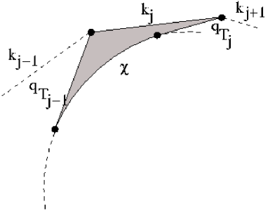
Figure 1: A plaquette bordered by $q_{Tj}$, $q_{Tj+1}$ , $k_{j}$ and a hyperbolic segment from the $\mathcal{X}$-curve, as described in the text.

The $\Delta\lambda_{j}$ defined in this way is the size of a subarea just as the total $\lambda$ represents the area spanned between the $\mathcal{X}$ and the directrix curves. In Fig. 1 we exhibit such a region bordered by the “initial” $q_{Tj-1}$ and the “final” $q_{Tj}$ together with a hyperbolic segment from the $\mathcal{X}$-curve and the gluon energy–momentum vector $k_{j}$ from the directrix.

If we define $\gamma_{0}\equiv 1$ and the vectors $\acute{k_{j}}\equiv\frac{1}{2}k_{j}(1+\gamma_{j})$, then it is easy to see that the vector $q_{Tj}$ is a weighted sum of the $\acute{k_{l}}$ vectors ($l\leq j$). The weight for any vector $\acute{k_{m}}$ is exponentially suppressed with $\sum_{l=m}^{j-1}\Delta\lambda_{l+1}$.

To see that $\Delta\lambda_{j}$ as defined in Eq. (19) actually has the meaning of a rapidity we go to the rest frame of the vector $q_{Tj-1}$ and assume for simplicity that it has the length $m_{0}$. Further assume that the lightlike vector $k_{j}$ is directed along the $3$-axis with the length $\omega$ so that $\Delta\lambda_{j}=\ln(1+\omega/m_{0})$. Then it is easy to show that the “next” $q_{T}$-vector $q_{Tj}$ will have the lightcone coordinates along the $3$-axis equal to $(m_{0}\exp(\Delta\lambda_{j}),m_{0}\exp(-\Delta\lambda_{j}))$, i.e. the $q_{T}$ vector has been accelerated from rest to the rapidity $\Delta\lambda_{j}$ by “the step” $k_{j}$ along the directrix. The corresponding segment of the $\mathcal{X}$-curve is a part of a hyperbola.

For sufficiently well ordered emissions and a resolution scale much smaller than the smallest transverse momentum present, the last term (Eq. (12)) will dominate in Eq. (11) and therefore $\lambda(m_{0}=\frac{1}{2}k_{\perp})$ will be approximately equal to $\ell(k_{\perp})$ defined in Eq. (5).

From the definition in Eq. (19) it is easy to show (cf. the definition of the vectors $q_{Tj}$ in Eq. (2.2)) that the argument in the logarithm of the $\Delta\lambda_{j}$ is equal to $(1+s_{j-1,j}/4m_{0}^{2})$ plus terms down by at least a factor of $\gamma$. From the definition of the local $k_{t}$ variables, Eq. (6), we may also conclude that

$$k_{tj}^{2}<\frac{s_{j-1,j}s_{j,j+1}}{(s_{j-1,j}+s_{j,j+1})}$$ (20)

and consequently we obtain

$$\Delta\lambda_{j} > \ln(\frac{s_{j-1,j}}{4m_{0}^{2}})=\ln(\frac{s_{j-1,j}}{k_{\perp}^{2}})\equiv\ell_{j-1,j}$$

$$\ln(\frac{k_{tj}^{2}}{k_{\perp}^{2}}) < \min(\ell_{j-1,j},\ell_{j,j+1})$$ (21)

This implies that there is a minimum positive value of $\Delta\lambda$, if a procedure to exclude or filter out emissions creating gluons with $k_{t}<k_{\perp}$ has been used.

3 The Properties of the $\Delta\lambda$ Distributions

We will now exhibit a very noticeable regularity of the dipole cascades, cf. Fig. 2. In this figure, we show a plot of the average number of gluons as a function of $k_{\perp}$, $n(k_{\perp})$, versus $\ell(k_{\perp})$ for $e^{+}e^{-}$-events with $\sqrt{s}=200$ GeV and for a range of values of $k_{\perp}$ from $4$ down to $1$ GeV. We have switched off the gluon splitting process so that we end up with one colour connected set of partons.

There are several interesting properties of this plot:

• There is a linear correlation between the average gluon multiplicity $\langle n(k_{\perp})\rangle$ and the phase space variable $\ell(k_{\perp})$ inside a very narrow band. The fact that the different lines obtained for different values of $k_{\perp}$ are so close to each other means that the slope of this linear correlation is rather insensitive to changes in the ordering variable in this range. It should be noted that the $\ell(k_{\perp})$-distributions are widely varying for these $k_{\perp}$-values as we show in Fig. 3. We have used a running coupling (with ${\Lambda_{QCD}}=0.22$ GeV, i.e. the default value in Ariadne). The region with $\ell(k_{\perp})>20$ is mainly populated by the results from small $k_{\perp}$-values, $k_{\perp}<2$ GeV.

• We find that the linear correlation in Fig. 2 is independent of the cms energy (we have used different cms energies ranging from $40$ GeV and up to even $2000$ GeV, though for small energies there are too few gluons emitted to allow detailed studies), cf. Fig. 4. Not only do we find a linear correlation at each value of cms energy (when the number of gluons is more than 2), the slope of the correlation varies rather weakly with respect to energy. This property is also not a function of the total thrust, or the presence of particularly hard emissions (e.g. gluon of $k_{\perp}>7$ GeV for $\sqrt{s}=200$ GeV). There is a minimum value of $\ell\simeq 10$, corresponding to no gluon emission (for $k_{\perp}=1$ GeV and $\sqrt{s}=200$ GeV), and there is a (small) transition region for a few more units, until the number of gluons exceeds two. But after that $dn/d\ell$ is a constant.

• As a consistency check we have used two procedures for sampling the events. It is possible to run the parton cascade in Ariadne down to a certain value of the ordering variable $k_{\perp}$, i.e. emit all gluons with larger $k_{\perp}$’s, sample the emerging directrix and investigate its properties, e.g. calculate the number of gluons emitted to that point, $n(k_{\perp})$, the total length of the $\mathcal{X}$-curve, $\ell(k_{\perp})$, the individual $\Delta\lambda(m_{0})$’s and the local $k_{t}$’s. After that we may continue the cascade for the same event down to smaller $k_{\perp}$-values and do the same exercise. Another possibility is to run the cascade down to a certain value $k_{\perp}\equiv{k_{\perp}}_{cut}$ and collect a large sample of events to investigate. After this we can pick a new value of ${k_{\perp}}_{cut}$ and repeat the process. The result in Fig. 2 does not depend upon which of the two methods for sampling the events we use.

Figure 2: The figure shows a plot of $\langle n(k_{\perp})\rangle$ versus $\ell(k_{\perp})$ for an $e^{+}e^{-}$-event with $\sqrt{s}=$ 200 GeV from Ariadne.

Figure 3: The $\ell(k_{\perp})$-distribution for different $k_{\perp}$-values at $\sqrt{s}=$ 200 GeV.

Figure 4: The figure shows a plot of $\langle n(k_{\perp})\rangle$ versus $\ell(k_{\perp})$ ($k_{\perp}=1.0$ GeV) for different cms energies from Ariadne.

  Figure 5: The figure to the left shows a plot of $\langle n(k_{\perp})\rangle$ versus $\ell(k_{\perp})$ for an $e^{+}e^{-}$-event with $\sqrt{s}=$ 200 GeV from Pythia. The figure to the right shows $\langle n(k_{\perp})\rangle$ $\pm$ $\sigma$ versus $\ell(k_{\perp})$ at $\sqrt{s}=$ 200 GeV, $k_{\perp}=$ 1.0 GeV for coherent and incoherent showers in Pythia.

We observe the same effect in the parton shower in Pythia as in Ariadne. The ordering variable in Pythia is the parton virtuality $Q^{2}$, and the variable $\hat{k}_{\perp}^{2}=z(1-z)Q^{2}$ (where $z$ is the lightcone fraction taken by the emitted parton) is used as the argument for the running coupling. This is a good approximation for the transverse momentum in the case of massless parton kinematics. However, since transverse momentum itself is not the ordering variable in this case, there is no real lower limit to it. Therefore, in order to make the comparisons we filtered the events obtained from Pythia and combined partons such that all gluons had $k_{t}$ above a certain value proportional to $Q$.

It is then possible to use Pythia to obtain an inclusive sample of $n_{g}(CQ)$ and $\ell(CQ)$. We just note that it is possible to tune the constant $C$ such that, as shown in Fig. 5, there is the same $dn/d\ell$ as in Ariadne. We find that $C\approx 0.5$

It is possible to switch off the coherence conditions in the parton shower in Pythia, since the strong angular ordering is implemented only after the generation using the ordering variable $Q^{2}$. We show the effect of this feature in Fig. 5. For the same $C$ we obtain many more partons per unit phase space for an incoherent shower, although they still show a linear correlation to the $\ell$-measure.

The linear relation between $\langle n\rangle$ and $\ell$ can be understood as follows. If one considers a variable such as $\ell$ defined as in Eq. (5) where the parts $\Delta\ell_{j}$ are distributed with the averages $\mu_{j}$ and the variances $\sigma^{2}_{j}$, then $\ell$ itself will mostly have a gaussian distribution according to the central limit theorem. The average is $\bar{\mu}=\sum\mu_{j}$ and the variance $\bar{\sigma^{2}}=\sum\sigma^{2}_{j}$. The numbers $\bar{\mu}$ and $\bar{\sigma^{2}}$ are in general well-defined for large $n$ unless the values of the $\Delta\ell_{j}$ are correlated. We find that the $\Delta\ell_{j}$’s indeed show very little correlation, even between adjacent dipoles, cf. Fig 6. We also find that the average $\mu_{j}$ shows only a weak dependence upon the total number of gluons in the event, n, for a wide range of n.

Figure 6: Scatter plot of two adjacent $\Delta\ell$ values

Figure 7: The $\frac{dP}{d(\Delta\ell)}\equiv P_{\ell}(\Delta\ell)$-distribution from Ariadne.

We will therefore go over to the investigation of the distribution of the $\Delta\ell_{j}$ defined in Eq. (5). We notice that the first and the last term in Eq. (5) are different from the other terms in one important aspect. They are contributions from dipoles involving a quark or an antiquark (with different colour charges than gluons), whereas all the other terms come from purely gluonic dipoles. It turns out that the dipoles at the ends have slightly different distributions than all the rest. However, if the gluon splitting process is switched off, there are only two such dipoles in an event. This means that we can write for the average $\bar{\mu}=2\langle\mu_{{\mathrm{q}}}\rangle+(n-1)\langle\mu_{\mathrm{gg}}\rangle$. In Fig. 4 we see this effect clearly, because it is only for $n>2$ that we find a constant slope, i.e. when we have purely gluonic dipoles present. The properties we noted above are about variation of the number of gluons or dipoles with respect to $\ell(k_{\perp})$ and the stability of the slope of the correlations, and should correspond to the properties of purely gluonic dipoles. Therefore, from now on we will not include the very first and the very last $\Delta\ell$-values in the investigations. We have seen that purely gluonic dipoles, irrespective of their position along the directrix, have the same distribution in size. In Fig. 7, we show the distribution $\frac{dP}{d(\Delta\ell)}\equiv P_{\ell}(\Delta\ell)$ from Ariadne and observe that:

Figure 8: The average value of $\Delta\ell$ as a function of $\kappa\equiv\ln(k_{\perp}^{2}/\Lambda^{2})$. Note that the variation in the average $\Delta\ell$ in the figure is much smaller than the width of the distribution of $\Delta\ell$ as seen in Fig. 7.

• The distribution $P_{\ell}$ has an average $\mu$ and a variance $\sigma^{2}$, consistent with the results in Fig. 2. We have found that it is independent of the cms energy, of the global event variables like thrust and the total $\ell$-value for the event, and also of hard gluon emissions.

• The distribution $P_{\ell}$ is rather insensitive to the value of $k_{\perp}$. In Fig. 8, we show the average value of $\Delta\ell$ as a function of $\kappa\equiv\ln(k_{\perp}^{2}/\Lambda^{2})$ and we find that it changes about 5 %, when the ordering variable goes from $0.8$ to $3$ GeV.

  

  Figure 9: The figure shows the average $\Delta\ell$ (and the standard deviations around it) for chains of $n$ connected $\Delta\ell$ called $a(n)$ ($a(n)\equiv\langle\sum_{j=1}^{n}\Delta\ell_{j}\rangle$). The statistics is collected from events with a fixed number of gluons.

• There are no noticeable correlations between adjacent $\Delta\ell$’s as we have noted before. In Fig. 6, we show the scatter plot beween two adjacent $\Delta\ell$, taken from stochastically chosen pairs in many different events. In Fig. 9, we show the values of the average $a(n)$ (defined as $a(n)\equiv\langle\sum_{j=1}^{n}\Delta\ell_{j}\rangle$), and the standard deviations around it, for chains of $n$ connected $\Delta\ell$. For this figure the statistics was collected from events with a fixed number of gluons.

• In order to further investigate the independence of the $\Delta\ell$ values in an event we have examined events containing a fixed number ($N$) of gluons. We may then ask about the multiplicity distribution, $\hat{P}(N_{\Delta})$, of events with $N_{\Delta}$ values of $\Delta\ell\leq\Delta$. We find a binomial distribution with the mean $Np$ and variance $Np(1-p)$ where $p=\int_{0}^{\Delta}dxP_{\ell}(x)$ as expected from uncorrelated dipoles. We have also investigated the average number of $\Delta\ell$-values, which are consecutive and satisfy $\Delta\ell\leq\Delta$. We find a geometric distribution, weighted with the average number of $\Delta\ell$ not fulfilling the condition (which is, once again, expected when we have uncorrelated dipoles). We also find that the distribution $P_{\ell n}$ obtained from the sum of the lengths of $n$ consecutive $\Delta\ell$ is an $n$-fold convolution of the distribution $P_{\ell}$.

  Figure 10: The figure to the left shows the $P_{\ell}(\Delta\ell)$-distribution from Pythia compared to the distribution obtained from Ariadne. The figure to the right shows the corresponding plot for the $P_{\lambda}(\Delta\lambda)$ distribution.

The corresponding results in Pythia are very similar to the results in Ariadne (with the appropriate choice of the constant $C$ as discussed above). To the left in Fig. 10 , we show the distributions from Pythia and note that Pythia is somewhat more concentrated towards small $\Delta\ell$ values and also has a somewhat wider tail so that the average values are the same as in Ariadne. The “incoherent” option gives a much more narrow distribution centred around smaller values, as expected.

It is also possible to investigate the distributions in terms of the $\lambda$-measure defined in Eq. (19). In Fig. 10 to the right, we show two distributions (one from Ariadne and one from Pythia), to be called $P_{\lambda}(\Delta\lambda)$ using as before $2m_{0}=k_{\perp}=CQ$ where $m_{0}$ is the argument of the $\lambda$-measure. Once again we find the same properties as for the distributions $P_{\ell}(\Delta\ell)$.

We conclude that, inside the whole region relevant to the hadronisation procedure in String Fragmentation, the partonic states are dominated by this structure of independent entities. It is tempting to consider them as a kind of collective variables for the QCD force fields. The $\Delta\ell$ variables represent the local size of the dipoles between adjacent parton energy–momentum vectors, whereas the $\Delta\lambda$ values correspond to a similar although more non-local property depending upon a set of adjacent vectors.

These properties of the distributions of $\Delta\ell$’s are properties of gluonic dipoles, and result from perturbative QCD. In the next section we will make models in the LLA and the MLLA schemes based on simple gain loss considerations on the dipole cascade model, and show that it is possible to understand many qualitative features of these distributions.

The $\Delta\lambda$’s on the other hand are complicated objects, and there is no obvious way to calculate their distributions except by relying on the similarity between the $\lambda$-measure and $\ell$. But the fact that there are as many $\Delta\lambda$’s as $\Delta\ell$’s, and the $\Delta\lambda$’s have parallels for each of the properties of the $\Delta\ell$’s discussed here, lead us to introduce the notion of Generalised Dipoles (GD) to be the “source” of the contributions to the $\Delta\lambda_{j}$’s. Whereas a dipole is spanned between two colour connected partons, a GD corresponds to one flat block or “plaquette” in the surface traced between the directrix and the $\mathcal{X}$-curve by the tangent to the $\mathcal{X}$-curve. Regularities in the properties of dipoles which are mirrored in the GD’s would be passed on to the hadronised state in a hadronisation scheme based on the $\lambda$-measure, such as the one introduced in [8].

4 Models to Describe The Dipole Distributions

4.1 A Simple Cascade Model

Multiplicity distributions were presented in the parton cascade formalism in [14] and in the dipole cascade formalism in [15] to leading logarithmic order. In this paper we will follow the approach presented in [16].

In order to provide a theoretical framework for our findingsin the previous section, we will consider an analytical model for a dipole cascade. We will assume that there is a distribution, $f(\mu,\kappa)d\mu$, that describes the dipoles with size $\mu$ at the scale $\kappa\equiv\ln(k_{\perp}^{2}/\Lambda^{2})$ (where $k_{\perp}$ is the ordering variable and $\mu\equiv\ln(M_{d}^{2}/k_{\perp}^{2})$, in terms of the dipole masses $M_{d}$). We will consider the change in $f$ when we make a small change in the scale $\kappa$. We note that $\mu+\kappa=ln\frac{M_{d}^{2}}{\Lambda^{2}}$ is independent of $\kappa$. If dipoles never decayed, the distribution $f(\mu,\kappa)$ would not change if $\mu+\kappa$ is kept constant as $\kappa$ varies. Therefore any change in the distribution along the lines $\mu+\kappa=constant$ must purely come from decays.

There are two contributions to this. A dipole of size $\mu$ may decay into two smaller dipoles. A dipole of size bigger than $\mu$ may decay such that one of the daughter dipoles is of size $\mu$. Gathering these terms together we get a partial integro-differential equation, cf. [16, 17], based upon Eq. 1 with $\alpha_{\mathrm{eff}}=\frac{\alpha_{0}}{\kappa}$ for gluonic dipoles ($\alpha_{0}=\frac{6}{11-2N_{f}/N_{c}}$ ):

$$Df\equiv\frac{\partial f}{\partial\kappa}-\frac{\partial f}{\partial\mu}=\frac{\alpha_{0}}{\kappa}\left[\mu f(\mu,\kappa)-2\int_{\mu}d\mu^{\prime}f(\mu^{\prime},\kappa)\right]$$ (22)

The factor of 2 in the contribution from the larger dipoles stems from the fact that we are only considering “central” or purely gluonic dipoles here. When a gluonic dipole decays, there are 2 equivalent ways to obtain a gluonic dipole of size $\mu$.

This integro-differential equation can be made into two coupled differential equations in terms of the first two moments of $f$, $N_{1}$ and $N_{2}$

$$N_{j}(\mu,\kappa) = \int_{\mu}d\mu_{1}(\mu_{1})^{j-1}f(\mu_{1},\kappa)$$

$$DN_{1} = -\frac{\alpha_{0}}{\kappa}(N_{2}-2\mu N_{1})$$

$$DN_{2} = -N_{1}+\frac{\alpha_{0}}{\kappa}\mu^{2}N_{1}$$ (23)

For the normalisation we note that $N_{1}(0,\kappa)$ is the total number of dipoles available at the scale $\kappa$, to be called $\bar{n}$ in this section. $N_{2}(0,\kappa)$ is their combined length, to be called $\bar{\ell}$. The equations for these quantities can be obtained directly from Eqs. (4.1) in the $LLA$-scheme:

$$\frac{d\bar{n}}{d\kappa} = -\frac{\alpha_{0}}{\kappa}\bar{\ell}$$

$$\frac{d\bar{\ell}}{d\kappa} = -\bar{n}$$ (24)

These equations are solvable in terms of combinations of the modified Bessel functions (cf. the next subsection) as soon as we have defined a “starting value”, $\kappa_{max}\equiv L_{0}$, for the cascade.

In order to solve the coupled equations in Eq. (4.1), we introduce the combination $g(\mu,\kappa)=N_{2}-\mu N_{1}$, which fulfils the equation:

$$Dg = \frac{\alpha_{0}}{\kappa}(\mu g)$$ (25)

with the boundary value

$$g(0,x) = \bar{\ell}(x)$$ (26)

It is related to $N_{1}$ through $N_{1}(\mu,\kappa)=-\frac{\partial}{\partial\mu}g(\mu,\kappa)$.

Including the boundary condition above, we obtain:

$$N_{1}(\mu,\kappa) = -\frac{\partial}{\partial\mu}\left\{\bar{\ell}(\mu+\kappa)\exp\left[-\int_{\kappa}^{\mu+\kappa}dy\frac{\alpha_{0}}{y}(\mu+\kappa-y)\right]\right\}$$ (27)

This is a derivative of two contributing factors. The first is $\bar{\ell}$ evaluated at $\mu+\kappa\equiv\ln(M_{d}^{2}/\Lambda^{2})$, i.e. at the largest $\kappa$ value where the dipole could have been produced. It is multiplied by the probability that the dipole has not decayed until $\kappa$. In field theoretical language this second contribution, the Sudakov form factor, corresponds to the sum of all the virtual corrections during the “lifetime” of the dipole. This Sudakov form factor can be easily calculated

$$S(\mu,\kappa) = \exp\left[-\int_{\kappa}^{\mu+\kappa}dy\frac{\alpha_{0}}{y}(\mu+\kappa-y)\right]=\frac{\exp(\alpha_{0}\mu)}{(1+\frac{\mu}{\kappa})^{\alpha_{0}(\mu+\kappa)}}$$ (28)

It fulfils

$$S(0,\kappa) = 1$$ (29)

$$\frac{\partial S}{\partial\mu}(\mu,\kappa) = -\alpha_{0}\ln(1+\frac{\mu}{\kappa})S$$

The derivative vanishes at $\mu=0$.

The distribution $f$ is obtained by a partial differentiation of $N_{1}$, cf. Eq. (4.1)

$$f(\mu,\kappa)=-\frac{\partial N_{1}}{\partial\mu}$$ (30)

so that using Eqs. (4.1), (27) and (29) we obtain:

$$f(\mu,\kappa) = [\bar{\ell}(L_{0},\mu+\kappa)\alpha_{0}\ln(1+\mu/\kappa)^{2}+$$ (31)

$$2\bar{n}(L_{0},\mu+\kappa)\alpha_{0}\ln(1+\mu/\kappa)]S(\mu,\kappa)$$

The result can be understood in a simple and useful way. The logarithmic factors in the parenthesis are equal to

$$\alpha_{0}\ln(1+\mu/\kappa)=\int_{\kappa}^{\mu+\kappa}\frac{\alpha_{0}dx}{x}$$ (32)

i.e. the probability that there will be a dipole breakup somewhere between $\mu+\kappa$, the largest virtuality where a dipole with size $\mu$ at $\kappa$ can be produced, and $\kappa$, where it is found. There are two such factors multiplying all interior points in the dipoles at $\mu+\kappa$ , counted by $\bar{\ell}(\mu+\kappa)$, and there is one factor multiplying twice the number of dipoles at $\mu+\kappa$ (because if there is already a dipole one can keep either its “left” side or its “right” side and produce the “other” side of the dipole with size $\mu$ by a breakup in between). Finally, the Sudakov form factor describes the probability that there is no decay affecting the existence of the dipole at $\kappa$.

In the limit when $L_{0}\gg(\mu+\kappa)$, and $\mu+\kappa$ is significantly positive, the two functions $\bar{n}$ and $\bar{\ell}$ factorise and we may write in the $LLA$

$$\bar{n}(L_{0},x) \simeq V(L_{0})(x)^{-\frac{1}{4}}\exp(-2\sqrt{\alpha_{0}x})$$ (33)

$$\bar{\ell}(L_{0},x) \simeq \sqrt{x/\alpha_{0}}\bar{n}(L_{0},x)$$

Figure 11: The $f_{\kappa}(\mu)$ function, obtained from Eq. 31, normalised to unity.

In Fig. 11, we show the function $f_{\kappa}(\mu)$, obtained from $f$ in Eq. (31) by normalising it to unity, for a set of values of the parameter $\kappa$. There is a weak dependence upon the ordering variable $\kappa$ and for large $\mu$-values it has an essentially exponential falloff with a slope very similar to the ones we find in the distributions $P_{\ell}(\Delta\ell)$ and $P_{\lambda}(\Delta\lambda)$ in Section 3.

For small values of $\mu$ there are quantitative differences. The reason is that the $LLA$ is not sufficient to describe the behaviour of small dipoles. In that case it is necessary to include both the contributions from the $(\sum_{p})$ term in the dipole cross section in Eq. (1), and also to take into account the recoil contributions which are particularly noticeable for small dipoles. We will consider this question in the next subsection.

4.2 The $MLLA$ and Earlier Investigations

In the so-called Modified Leading Log Approximation, subleading effects from the polaristaion sum are included [7, 18]. In general, the assumptions have been that the cms energy $\sqrt{s}$ (or rather its logarithm $L\equiv\ln(s/\Lambda^{2})$) is very large and that the main contributions from the cascades will come from well-ordered emissions, i.e. that $k_{\perp j}\gg k_{\perp j+1}$ (at least for adjacent emissions).

Using this approximation, it is possible to write out analytical equations for the expected changes in the average $\ell$ (to be called $\bar{\ell}(\kappa)$) and the average $n$ (similarly $\bar{n}(\kappa)$) for a given ordering variable $\kappa\equiv\ln(k_{\perp}^{2}/\Lambda^{2})$ [7, 17, 18]:

$$\frac{d\bar{\ell}}{d\kappa} = -\bar{n}$$

$$\frac{d\bar{n}}{d\kappa} = -\alpha_{\mathrm{eff}}(\bar{\ell}-\bar{n}\delta)$$ (34)

Eqs. (4.2) are simplified versions of the Modified Leading Log Approximation (MLLA) formulae. A more elaborate treatment should include the difference between the quark and antiquark endpoint dipoles with a different effective coupling $\alpha$ and a different correction $\delta$, cf. [18], but these are small corrections if the starting value $L=\ln(s/\Lambda^{2})$ is large.

The interpretation is that in a step $d\kappa$, $\bar{\ell}$ changes by $\bar{n}$ contributions from the scale change according to Eq. (5), just like the second line in Eq. (4.1). Further, the change in $\bar{n}$ in that step is given by the coupling times the available phase space. This phase space is given by $\bar{\ell}$ to first approximation; but there is a correction from each dipole from the term $\sum_{p}$ in Eq. (1). The polarisation sum $\sum_{p}\simeq 2$ near the centre of a dipole but decreases in the neighbourhood of the emitters. It has been shown [18] that the suppression of emissions because of this can be approximated by (and this is essentially the MLLA) a constant decrease in the dipole size $\delta=11/6$ for gluonic dipoles (this number only depends upon the triple gauge boson vertex for 3 colours). In Eqs. (4.2) it is also assumed that the gluon splitting process $g\rightarrow q\bar{q}$ is neglected and therefore $\alpha_{\mathrm{eff}}\equiv\alpha_{0}/\kappa$ with $\alpha_{0}=6/11$ for all dipoles and not only the purely gluonic ones.

The decay of one dipole also affects the two adjacent ones due to recoils. A method to estimate this effect was suggested in [19]. Therefore an extra “loss-term” is added to the first line in Eq. (4.2):

$$\frac{d\bar{\ell}}{d\kappa}=-\bar{n}-C_{r}\frac{d\bar{n}}{d\kappa}$$ (35)

with a constant recoil correction estimated to be $C_{r}\simeq 2$.

These equations can be solved using the following combinations of the modified Bessel functions:

$$\mathcal{I}_{1}(x) = \sqrt{2}x^{\gamma/2}I_{\gamma}(2\sqrt{\alpha_{0}x})$$

$$\mathcal{I}_{2}(x) = \sqrt{2\alpha_{0}}x^{(\gamma-1)/2}I_{\gamma-1}(2\sqrt{\alpha_{0}x})$$ (36)

and similarly for $\mathcal{K}_{1}$ and $\mathcal{K}_{2}$ in terms of the exponentially falling Bessel function $K$. Note that they are normalised so that

$$\mathcal{I}_{1}(x)\mathcal{K}_{2}(x)+\mathcal{I}_{2}(x)\mathcal{K}_{1}(x)=x^{\gamma-1}$$ (37)

and that there are simple differential relations between them:

$$\frac{d\mathcal{I}_{1}}{dx} = \mathcal{I}_{2}(x)$$

$$\frac{d\mathcal{I}_{2}}{dx} = \frac{\alpha_{0}}{x}\mathcal{I}_{1}(x)+\frac{(\gamma-1)}{x}\mathcal{I}_{2}(x)$$ (38)

Similar relations hold for the exponentially falling modified Bessel function pair $(\mathcal{K}_{1},-\mathcal{K}_{2})$.

If we start the cascade at a large value of $L\equiv\ln(s/\Lambda^{2})\gg\kappa$ we obtain, with the boundary values $\bar{\ell}=0$ and $\bar{n}=1$ at $L$, the results:

$$a = L^{1-\gamma}\left[C_{r}\mathcal{K}_{2}(L)-\mathcal{K}_{1}(L)\right]$$ (39)

$$b = L^{1-\gamma}\left[C_{r}\mathcal{I}_{2}(L)+\mathcal{I}_{1}(L)\right]$$

$$\bar{n} = b\mathcal{K}_{2}(\kappa)-a\mathcal{I}_{2}(\kappa)$$

$$\bar{\ell}+C_{r}\bar{n} = a\mathcal{I}_{1}(\kappa)+b\mathcal{K}_{1}(\kappa)$$

using the notations $\gamma=1+\alpha_{0}(\delta+C_{r})$.

It is difficult to obtain an anlytically solvable partial integro-differential equation corresponding to Eq. (22). The method of moments runs into difficulties because the variation in the $\sum_{p}$ term in the cross section (Eq. (1)) affects the integral contribution, i.e. the gain from the decays of larger dipoles, in such a way that the equations for the first few moments are no longer independent of higher moments. Therefore, we will directly go over to the solution in Eq. (31) instead, and modify the ingoing terms according to the MLLA, keeping in mind the interpretation given there.

We assume that each dipole of size $\mu$ can decay only in the interior excluding a region $\delta/2$ on each extreme. Then the effective phase space at $(\mu+\kappa)$ in Eq. (31) is changed from $\ell(\mu+\kappa)$ into $[\ell(\mu+\kappa)-\delta\cdot n(\mu+\kappa)]$. A dipole of size $\mu$ is produced by a breakup first at a point $\kappa=\kappa_{1}$ and then at $\kappa_{2}<\kappa_{1}$. The region where the “no emission probability” is to be calculated in the Sudakov form factor is changed in the MLLA, first by a loss of $\delta/2$ at $\kappa_{1}$ and then by a loss of a further $\delta/2$ at $\kappa_{2}$.

$$S_{\kappa_{1},\kappa_{2}} = \exp\left(-\int_{\kappa}^{\kappa_{2}}\frac{\alpha_{0}dz(\mu+\kappa-\delta-z)}{z}\right)\exp\left(-\int_{\kappa_{2}}^{\kappa_{1}}\frac{\alpha_{0}dz(\mu+\kappa-\delta/2-z)}{z}\right)\times$$ (40)

$$\exp\left(-\int_{\kappa_{1}}^{\mu+\kappa}\frac{\alpha_{0}dz(\mu+\kappa-z)}{z}\right)=\left(\frac{\kappa_{1}\kappa_{2}}{\kappa^{2}}\right)^{\frac{\alpha_{0}\delta}{2}}S(\mu,\kappa)$$

where $S(\mu,\kappa)$ is the Sudakov form factor without the term $\delta$ as given in Eq. (28). Since this is a function of $\kappa_{1}$ and $\kappa_{2}$ now, we obtain, for the contribution to $f(\mu,\kappa)$ from situations where both gluons involved in a dipole are emitted below $\mu+\kappa$, the result:

$$f_{1} \equiv 2(\bar{\ell}-\delta\bar{n})(\mu+\kappa)\int_{\kappa}^{\mu+\kappa}\frac{\alpha_{0}d\kappa_{1}}{\kappa_{1}}\int_{\kappa}^{\kappa_{1}}\frac{\alpha_{0}d\kappa_{2}}{\kappa_{2}}S_{\kappa_{1},\kappa_{2}}$$ (41)

$$= (\bar{\ell}-\delta\bar{n})(\mu+\kappa)\frac{4\left((1+\mu/\kappa)^{\frac{\alpha_{0}\delta}{2}}-1\right)^{2}}{\delta^{2}}S(\mu,\kappa)$$

The fact that the first break may be either on the “left” or on the “right” side contributes a factor of $2$ in the above equation .

  Figure 12: The figure to the left shows the distribution $f_{\delta}(\mu,\kappa)$, obtained from the MLLA approach at $k_{\perp}=$$1GeV$, compared with the $P_{\ell}(\Delta\ell)$ distribution from Ariadne and Pythia (cf. Fig. 10). The figure to the right shows the average value of $\mu$ as a function of $\kappa$, from the same distribution $f_{\delta}(\mu,\kappa)$. In the figure to the right, we also compare with the average value of $\ell$ (cf. Eq. (2.2)) as a function of $\kappa$ obtained from Ariadne and Pythia, and we also include the standard deviation in the result from Pythia and Ariadne. This result is obtained using $\alpha_{0}=0.7$ and $C_{r}=2$ in the MLLA distribution as explained in the text.

In the same way, for the second contribution related to the number of dipoles at $\mu+\kappa$, ie the situations where only one gluon involved in a dipole is produced below the scale $\mu+\kappa$, we obtain,

$$f_{2}=\theta(\mu-\delta/2)\bar{n}(\mu+\kappa)\frac{4\left((1+(\mu-\delta/2)/\kappa)^{\frac{\alpha_{0}\delta}{2}}-1\right)}{\delta}S(\mu-\delta/2,\kappa)$$ (42)

In this case there can never be a breakup until the dipole size has at least reached $\delta/2$, because one of the end points is already fixed at the virtuality $\mu+\kappa$.

We note for consistency that the result $f_{\delta}\equiv f_{1}+f_{2}$ has the limit $f$ in Eq. (31) when $\delta$ vanishes. In Fig. 12, we show the result of this $MLLA$ version of the dipole size distribution. We have used a fixed value $\delta=11/6$ but we have allowed the parameters $\alpha_{0}$ and $C_{r}$ vary. The reason for allowing $\alpha_{0}$ to vary is that it is feasible to shut off the gluon splitting process in Ariadne, but the running coupling will always receive contributions from the different number of “active” flavours at different virtualities. From the figure to the left, we conclude that it is in between the distributions from Ariadne and Pythia for the central dipoles when we use $\alpha_{0}=0.70$ (i.e. for three to four active flavours), and $C_{r}=2$ (according to [19]). This result is rather insensitive to $C_{r}$ and it can therefore not be used as a test for the claims in [19]. We have also checked the dependence upon the ordering variable. In Fig. 12 to the right, we show that $f_{\delta}$ also exhibits a slow change of its average value as a function of the (relevant) ordering variable like the Ariadne and Pythia $P_{\ell}$ distributions.

5 Concluding Remarks

The number of gluons emitted above a certain value of the ordering variable shows an interesting linear correlation (with gaussian fluctuations) with the phase space available at that scale. We have called the phase space variable the $\ell$-measure in this paper to distinguish it from the $\lambda$-measure, which is an infrared stable generalisation of the $\ell$-measure, useful in the context of hadronisation.

Both these quantities are functions of not only the resolution scale ($k_{\perp cut}$ for a dipole cascade, $\Gamma_{0}$ in string fragmentation), but also of the precise geometry of the state under consideration. Therefore they change with every new gluon emitted in the system.

The resolution parameter relevant for hadronisation is a parameter fixed by the break-up properties of the string and the mass spectrum of the hadrons produced. The $\lambda$-measure is constructed in such a way that addition of gluons at transverse momenta much smaller than the scale $\Gamma_{0}$ does not change its value. In that way it is infrared stable.

However, since the resolution parameter for the $\ell$-measure is the transverse momentum of the gluon to be emitted, the transverse momenta of all gluons already emitted must be higher in an ordered dipole cascade. Therefore, the only kind of infrared stability relevant for this measure would be the stability, when the ordering variable, which is also the resolution parameter, is small. Technically this is not the case. However, since in this approach we will never compute phase space available at a value of the ordering variable below the $\Lambda_{QCD}$, there is an effective infrared stability for the phase space, if all local transverse momenta $k_{tj}$ are required to be above $k_{\perp}$. It is easily shown that the mass of any dipole with a gluon at one end is greater than the transverse momentum $k_{t}$ of that gluon, which in turn, will be greater than $\Lambda_{QCD}$. Besides, we must remember that it is kinematically not possible for dipoles of mass smaller than $2\Lambda_{QCD}$ to emit gluons above $\Lambda_{QCD}$.

The two measures discussed here are quite strongly related. If one keeps only the last (often the dominant) term in the argument of the logarithm in the $\lambda$-measure, one gets an expression very similar to the $\ell$-measure.

The linear correlation between the $\ell$-measure and the number of gluons is a direct consequence of the following facts that we have demonstrated. The $\ell$-measure is the sum of a series of terms $\Delta\ell_{j}$, one for each dipole. A given $\Delta\ell_{j}$ is the contribution from one particular dipole to the $\ell$-measure, and is in some sense the “size” of that dipole. There are two kinds of dipoles. The first kind involves either the quark or the antiquark energy–momentum. The second kind involves only the gluon energy–momenta. These two kinds of dipoles have different distributions in sizes.

It turns out that the size of the dipoles do not show any significant correlations. Therefore the $\ell$-measure of a state consisting of a certain number of dipoles, which is just the sum of the corresponding $\Delta\ell_{j}$’s, is distributed like the sum of several independent random variables, i.e. like a gaussian with a mean that is the sum of the means of the individual independent distributions. This shows up as a linear correlation between the number of partons and the $\ell$-measure.

More interesting than the linear relation is the stability of the slope of these lines, which represents the number of gluons per unit phase space, with respect to changes in global event parameters like cms energy or thrust and even with changes in the ordering variable. It seems that parton cascades tend to form structures at one (relative) size when sizes are measured with the $\ell$-measure with a resolution parameter proportional to the ordering variable. As we go down in the ordering variable, the running coupling should increase the number of emissions per unit phase space. However, the phase space variable itself scales appropriately to effectively absorb any increase of emissions per unit phase space.

We have also made another observation in this paper. Just like the $\ell$-measure, the $\lambda$-measure can be thought of as a sum of terms $\Delta\lambda_{j}$, one for each vector along the directrix in colour order. Out of the two vectors involved in a particular $\Delta\lambda_{j}$, only one is a vector along the directrix. The other vector, in a sense a cumulative variable, is a weighted average of the vectors $k_{i}$’s along the directrix with $i<j$.

It is interesting that all the properties of the $\ell$-measure we have discussed here are also reflected in the $\lambda$-measure. There is a similar linear correlation to the number of gluons, similar lack of correlation among adjacent terms and similar stability with respect to change of global event variables and the ordering variable. Partitioning the $\lambda$-measure into a series of $\Delta\lambda_{j}$’s corresponds to partitioning the surface spanned between the directrix and the $\mathcal{X}$-curve into a series of “plaquettes” or flat regions along the directrix. Each plaquette is spanned between a parton energy momentum vector $k_{j}$, a vector $q_{Tj-1}$ (weighted average of $k_{i}$’s along the directrix with $i<j$), another vector $q_{Tj}$ and a hyperbolic section of the $\mathcal{X}$-curve. The size of the plaquette $\Delta\lambda_{j}$ is the length of the section of the $\mathcal{X}$-curve, and is determined by $k_{j}$ and $q_{Tj-1}$. Since these plaquettes share so many properties with dipoles, we will call them “Generalised Dipoles”.

We note in passing that the possibility of partitioning the contributions to the $\lambda$-measure as contributions from connected flat regions has an interesting consequence for the fragmentation of a string according to the Lund model area law. Such a fragmentation scheme was presented in [8], which was closely related to the $\lambda$-measure and the $\mathcal{X}$-curve. Particle production in this scheme can be thought of as partitioning the plaquettes mentioned here into smaller plaquettes, one for each hadron. Since the hadron energy–momenta will mostly come from these flat regions in the string, particles stemming from one GD will have energy–momenta aligned in a plane in Minkowski space, up to transverse momentum fluctuations. We have found such chains of particles and examined their properties. These chains, which we will call “coherence chains” are important for the study of Bose Einstein correlations in the Lund Model for multigluon systems, which we will elaborate on in a forthcoming publication.

We have also presented here an analytical model for the observations we have made about dipoles, in the LLA and MLLA schemes. There are limitations to this approach, since complications such as the polarisation sum make it very difficult to obtain differential equations which can be solved analytically. Nevertheless, our analysis based on simple gain-loss considerations broadly reproduces the qualitative features of the observations.

6 Acknowledgements

We would like to thank G. Gustafson, T. Sjöstrand and L. Lönnblad for helpful discussions. This work was completed by S. Mohanty and F. Söderberg, about two months after the untimely death of our collaborator Bo Andersson.

References

- [1] G. Gustafson, U. Pettersson Nucl. Phys. B306 (1988) 746
- [2] L. Lönnblad, Computer Phys. Commun. 71 (1992) 15
- [3] G. Corcella, I.G. Knowles, G. Marchesini, S. Moretti, K. Odagiri, P. Richardson, M.H. Seymour and B.R. Webber J. High Energy Phys. 0101 (2001) 010
- [4] T. Sjöstrand, P. Edén, C. Friberg, L. Lönnblad, G. Miu, S. Mrenna and E. Norrbin, Computer Phys. Commun. 135 (2001) 238
- [5] X. Artru, Phys. Rept. 97 (1983) 147
- [6] B. Andersson, G. Gustafson and B. Söderberg, Z. Phys. C20 (1983) 317
- [7] Yu.L. Dokshitzer, V.A. Khoze, A.H. Mueller and S.I. Troyan, Basics of Perturbative QCD (Edition Frontières 1991).
- [8] B. Andersson, S. Mohanty and F. Söderberg, Eur. Phys. J. C21 (2001) 631
- [9] B. Andersson, G. Gustafson, P. Dahlqvist, Nucl. Phys. B328 (1989) 76
- [10] G. Gustafson and A. Nilsson, Z. Phys. C52 (1991) 553
- [11] Ya.I. Azimov et al. Phys. Lett. B165 (1985) 147
- [12] L. Lönnblad, hep-ph/0112284.
- [13] B. Andersson, P. Dahlqvist and G. Gustafson, Z. Phys. C44 (1989) 455;Z. Phys. C44 (1989) 461
- [14] Yu.L. Dokshitzer, V.S. Fadin, V.A. Khoze, Z. Phys. C15 (1982) 325; A. Bassetto, M. Ciafaloni, G. Marchesini, A.H. Mueller, Nucl. Phys. B207 (1982) 189
- [15] B. Andersson, P. Dahlqvist and G. Gustafson, Phys. Lett. B214 (1988) 604
- [16] B. Andersson , Nucl. Phys. B360 (1991) 109
- [17] B. Andersson, The Lund Model, (Cambridge University Press 1998)
- [18] G. Gustafson, Nucl. Phys. B392 (1993) 251; G. Gustafson, M. Olsson, Nucl. Phys. B406 (1993) 293
- [19] P. Edén, G. Gustafson, J. High Energy Phys. 09 (1998) 015