DESY 02-084

NBI-HE-02-08

hep-ph/0207023

July 2002

Non-thermal Leptogenesis from the Heavier Majorana Neutrinos

T. Asaka^a,,  H. B. Nielsen^a,b, and  Y. Takanishi^a,b,

^a Deutsches Elektronen-Synchrotron DESY,
Notkestraße 85,
D-22603 Hamburg,
Germany
^b The Niels Bohr Institute,
Blegdamsvej 17,
DK-2100 Copenhagen Ø,
Denmark

We investigate a scheme for making leptogenesis by means of the $CP$ violating decays of the seesaw Majorana neutrinos proposed by Fukugita and Yanagida. However, in order to avoid the wash-out of the produced lepton number we propose the production of the Majorana neutrinos to occur non-thermally and sufficiently late. After this time, in consequence, the $B-L$ (baryon minus lepton) quantum number becomes a good “accidental symmetry” protecting the asymmetry produced. This non-thermal leptogenesis at late time is realized by a boson decaying into the Majorana neutrinos with a long lifetime. Suggestively this boson could correspond to a scalar field which causes the cosmic inflation, the inflaton, and thus its decay means really the reheating of the Universe. We find that this mechanism works well even if the lightest Majorana neutrinos are not produced sufficiently or not present, and the decays of the heavier seesaw Majorana neutrinos can be responsible to the baryon asymmetry in the present Universe, as we illustrate by the example of the family replicated gauge group model.

PACS numbers: 12.15.Ff, 13.35.Hb, 13.60.Rj, 14.60.St.
 Keywords: Non-thermal leptogenesis, Inflation, Seesaw mechanism, Family replicated gauge group model.

1 Introduction

Matter-antimatter asymmetry in the present Universe is one of the biggest puzzles in particle physics as well as in cosmology. This baryon asymmetry is usually expressed by the ratio of baryon (minus anti-baryon) number density $n_{B}$ to the entropy density $s_{0}$ in the present Universe as [1]

$$\frac{n_{B}}{s_{0}}=(3.7-8.8)\times 10^{-11}\hskip 5.69054pt.$$ (1)

It is only one, but mysterious, number in nature which we would like to understand. If our Universe experienced the inflationary stage in the beginnings of the history, the primordial baryon asymmetry would be diluted away and be essentially zero. The observed asymmetry in Eq. (1) should, therefore, be generated after the inflation. Such a generation mechanism is called baryogenesis and various scenarios have been proposed so far.

Evidence of the neutrino oscillations gives an important clue for baryogenesis, since Fukugita and Yanagida [2] proposed that lepton-number violation in nature might account for the present baryon asymmetry. The experimental data suggest tiny but non-zero masses for the neutrinos. Introducing the right-handed Majorana neutrinos having heavy masses is the natural set up to explain such neutrino masses through the seesaw mechanism [3]. If this is the case, the lepton number violation which is crucial for leptogenesis is naturally explained. In fact, non-equilibrium decays of Majorana neutrinos can produce a lepton number in the early Universe, which is partially converted into a baryon number through the electroweak sphaleron processes [5]. Therefore, the Fukugita-Yanagida mechanism [2], called leptogenesis, is probably the most attractive possibility to generate dynamically the observed baryon asymmetry in the present Universe.

There is a variety of scenarios for leptogenesis in the literature [2, 6, 7, 8, 9]. Here we restrict ourselves to leptogenesis via decays of the seesaw Majorana neutrinos ($N_{i}$: $i=1,2,3$) having the hierarchical masses $M_{3}\!\gg\!M_{2}\!\gg\!M_{1}$. It is usually considered that the decays of the lightest Majorana neutrinos $N_{1}$ are responsible for the present baryon asymmetry, although the decays of $N_{2}$ and $N_{3}$ also generate a lepton asymmetry. This is because the $N_{1}$, having the lightest mass, can remain in thermal equilibrium after the decays of $N_{2}$ and $N_{3}$, and may induce additional rapid processes changing the lepton number (other than the sphaleron process). These processes wash out the lepton asymmetry from $N_{2}$ and $N_{3}$ “too much” to make $N_{2}$ and $N_{3}$ work as the producers of baryon number [10], and hence the resultant asymmetry only comes from the decays of $N_{1}$.

In this paper, however, we point out that the decays of the heavier Majorana neutrinos $N_{2}$ and $N_{3}$ can be a dominant source of the present baryon asymmetry if they are produced non-thermally and also at very late time. The $N_{2}$ and $N_{3}$ produced non-thermally decay immediately after the production and generate the lepton asymmetry through the Fukugita-Yanagida mechanism. Furthermore, this production time is so late that the cosmic temperature is low enough to prevent thermalization of the $B-L$ (baryon minus lepton) asymmetry due to the lightest Majorana neutrinos $N_{1}$ as well as the wash-out processes caused by the existence of $N_{1}$. As a result, after that time the $B-L$ quantum number becomes a good “accidental symmetry”, which ensures the sphaleron conversion from the lepton asymmetry from $N_{2}$ and $N_{3}$ into the baryon asymmetry. This scheme is easily realized by a scalar field which dominates the energy of the Universe when it decays into the Majorana neutrinos with a long lifetime. Suggestively this boson could be described by a scalar field which causes the cosmic inflation, the inflaton, and thus its decay means really the reheating of the Universe [7].

The leptogenesis picture by the heavier Majorana neutrinos produced non-thermally in inflaton decays works well even if the leptogenesis by the $N_{1}$ decays is ineffective and also even if the $N_{1}$-neutrinos are absent in the early Universe. This means that our proposed scheme for the leptogenesis can be applied to a wider class of models. For example, we illustrate it in the family replicated gauge group model [11, 12] in which all the lepton and quark masses and mixing angles are well fitted order of magnitudewise. The proposed leptogenesis is well suited for this model, since the leptogenesis by the decays of $N_{1}$ is not sufficient to explain the phenomenological baryon asymmetry in this model. It is found that the proposed leptogenesis works well even in this model and also, interestingly, we can determine values of the reheating temperature as well as the inflaton mass from the present baryon asymmetry using this family replicated gauge group model.

The organization of this paper is as follows: In Section 2 we briefly review the leptogenesis by using the inflaton decays and we discuss the possibility of the baryon asymmetry generated by the decays of the heavier Majorana neutrinos. In Section 3 we review the family replicated gauge group model in which we illustrate our idea. In Section 4 we then derive the $B-L$ asymmetry obtainable by the proposed ideas. Some problems of naturalness of the rather isolated inflaton or just scalar needed are discussed in Section 5 by suggesting some possible – speculative – solutions. Our conclusions go into Section 6.

2 Leptogenesis in the inflaton decays

Let us start by explaining briefly the leptogenesis in inflaton decays scenario (see Ref. [7]). After de Sitter expansion of inflation ends, the inflaton decays, when the Hubble parameter of the Universe, $H$, becomes comparable to the decay width of the inflaton $\Gamma_{\phi}$. The vacuum energy of the inflaton $\phi$-field is completely released into decay products, and the Universe is reheated through their thermal scattering. The temperature at this time, the reheating temperature, $T_{R}$, is given using $\Gamma_{\phi}$ by

$$T_{R}=0.55\sqrt{M_{*}\Gamma_{\phi}}\hskip 5.69054pt,$$ (2)

where $M_{*}=2.4\times 10^{18}~{}\mbox{\rm GeV}$ is the reduced Planck mass.

We consider the seesaw Majorana neutrinos $N_{i}$ ($i=1,2,3$) produced by the decays of the inflaton $\phi$. If $N_{i}$ are produced “non-thermally”, the ratio between the number density of produced $N_{i}$ and the entropy density $s$ is estimated to be

$$\frac{n_{N_{i}}}{s}={\rm Br}_{i}\,\frac{3\,T_{R}}{2\,m_{\phi}}\hskip 5.69054pt,$$ (3)

where ${\rm Br}_{i}$ denotes the branching ratio of the decay channel $\phi\rightarrow N_{i}\,N_{i}$. When the decay rate of $N_{i}$ is much larger than $\Gamma_{\phi}$, the $N_{i}$ decays immediately after being produced by the inflaton decays. (As we shall discuss later, we are interested in low reheating temperatures which ensure this condition.)

Decays of Majorana neutrinos $N_{i}$ break the lepton-number conservation and have the $CP$ violation. There are two classes of decay channels:

$$N_{i}\rightarrow\phi_{\rm\scriptscriptstyle WS}+\ell\hskip 5.69054pt,~{}~{}~{}~{}N_{i}\rightarrow\phi_{\rm\scriptscriptstyle WS}^{\dagger}+\overline{\ell}\hskip 5.69054pt,$$ (4)

where $\phi_{\rm\scriptscriptstyle WS}$ and $\ell$ denote the Weinberg-Salam Higgs and lepton doublets in the Standard Model, respectively. The lepton asymmetry generated by $N_{i}$ decays can be expressed by

$$\epsilon_{i}\equiv\frac{\Gamma(N_{i}\rightarrow\phi_{\rm\scriptscriptstyle WS}+\ell)-\Gamma(N_{i}\rightarrow\phi_{\rm\scriptscriptstyle WS}^{\dagger}+\overline{\ell})}{\Gamma(N_{i}\rightarrow\phi_{\rm\scriptscriptstyle WS}+\ell)+\Gamma(N_{i}\rightarrow\phi_{\rm\scriptscriptstyle WS}^{\dagger}+\overline{\ell})}\hskip 5.69054pt.$$ (5)

Just after the reheating completes, we obtain the lepton asymmetry induced by $N_{i}$ decays as

$$\frac{n_{L}}{s}=\sum_{i=1}^{3}\ \epsilon_{i}\,{\rm Br}_{i}\,\frac{3\,T_{R}}{2\,m_{\phi}}\hskip 5.69054pt.$$ (6)

We will assume for a while an accidental $B-L$ conservation (in the sense that it is not imposed upon the model, but comes out). If the lepton asymmetry in (6) is produced well before the electroweak phase transition of the thermal history, i.e., $T_{R}\gg 100~{}\mbox{\rm GeV}$, the $B$ and $L$ conversion by the sphaleron process is active, and it brings a part of this lepton asymmetry into the baryon asymmetry as [13]

$$\frac{n_{B}}{s}=-\,\frac{28}{79}\,\frac{n_{L}}{s}\hskip 5.69054pt.$$ (7)

Here we have assumed that there is only one weak Higgs doublet. Finally, we obtain the following expression of the produced baryon asymmetry [7]

$$\frac{n_{B}}{s}=-\,\frac{42}{79}\,\sum_{i=1}^{3}\,\epsilon_{i}\,{\rm Br}_{i}\,\frac{T_{R}}{m_{\phi}}\hskip 5.69054pt.$$ (8)

Now we are at the point of justifying the assumptions which we have made in the above discussion. First, the production of $N_{i}$ in the inflaton decays is available only when

$$m_{\phi}>2\,M_{i}\hskip 5.69054pt.$$ (9)

Second, the estimation of the lepton asymmetry in Eq. (6) is obtained under the requirement that the $N_{i}$ are produced non-thermally by the inflaton decays, which leads to the following condition on the reheating temperature

$$T_{R}<\kappa_{i}\,M_{i}\hskip 5.69054pt,$$ (10)

where $\kappa_{i}$ are constants of order one defined by the decoupling temperatures of $N_{i}$ to be $T_{i}^{dec}=\kappa_{i}M_{i}$. Therefore, considering the inflation model satisfying the conditions (9) and (10), the decays of the Majorana neutrinos $N_{i}$ generate the lepton asymmetry which is given in Eq. (6) just after the reheating.

However, the lepton asymmetry might be washed out, after it is produced, by the lepton-number violating processes. The most dangerous ones are the processes mediated by $N_{1}$, since $N_{1}$ is the lightest Majorana neutrino, so that it survives and still can be produced in the thermal bath after $N_{2}$ and $N_{3}$ have disappeared. If those processes are well in thermal equilibrium the produced lepton asymmetry is washed-out strongly [10]. To avoid these wash-out processes, we have to invoke that the production of the Majorana neutrinos (i.e. lepton asymmetry) takes place at a sufficiently late time so that the wash-out processes have already decoupled and been ineffective. Thus, we have to consider sufficiently low reheating temperatures,

$$T_{R}<\kappa_{1}\,M_{1}\hskip 5.69054pt.$$ (11)

With such low reheating temperatures, the lighter Majorana neutrino(s) are completely decoupled from the thermal bath of the Universe, and the $B-L$ becomes a good “accidental symmetry” for $T<T_{R}$. The conditions Eqs. (9) and (11) justify our estimation of the baryon asymmetry in Eq. (8), by explaining why there is no wash-out effect.

It should be noted that Eq. (11) ensures the non-thermal production of the heavier Majorana neutrinos $N_{2}$ and $N_{3}$ if $m_{\phi}>2M_{3}$. This means that the decays of $N_{2}$ and $N_{3}$ can be dominant sources of the present baryon asymmetry (if $\epsilon_{2}\,{\rm Br}_{2}$, $\epsilon_{3}\,{\rm Br}_{3}\gg\epsilon_{1}\,{\rm Br}_{1}$). Further, this mechanism works even if there is no $N_{1}$, i.e., if ${\rm Br}_{1}=0$. This feature is completely different from the conventional thermal leptogenesis [6] where the lepton asymmetry is generated by the decays of $N_{2}$ ($N_{3}$) at the temperature of $T\sim M_{2}(M_{3})\gg M_{1}$, and hence the produced lepton asymmetry may be easily washed out and the resultant baryon asymmetry comes from the decays of the lightest Majorana neutrinos $N_{1}$.

These observations lead to that our proposed scheme for the leptogenesis can be applied to a wider class of models of the sort explaining fermion masses and mixings. In the next to next section, we will illustrate it in a specific example, a model presented in the following section.

3 Family replicated gauge group model

In this section we review briefly the family replicated gauge group model [11, 12]. This model is based on a large gauge group being the Cartesian product of family specific gauge groups, namely,

$${}\;\;\raisebox{3.87495pt}{$\times$}\raisebox{-2.15277pt}{$\!\!\!\!\!\!\!\!\scriptscriptstyle i=1,2,3$}\,(SMG_{i}\times U(1)_{\scriptscriptstyle B-L,i})\hskip 5.69054pt,$$ (12)

where $SMG_{i}$ denotes $SU(3)_{i}\times SU(2)_{i}\times U(1)_{i}$ (Standard Model gauge group), $U_{\scriptscriptstyle B-L,i}$ is $B-L$ gauge group, and $i$ denotes the generation. This group in Eq. (12) is represented only by representations that do not mix the different irreducible representation of the Standard Model and it breaks spontaneously down to the group $SU(3)\times SU(2)\times U(1)\times U(1)_{\scriptscriptstyle B-L}$ at the scale about $1$ to $2$ orders of magnitude under the Planck scale. The breaking to the Standard Model gauge group is supposed to occur by means of five Higgs fields which we have invented and denoted by the symbols $W$, $T$, $\rho$, $\omega$ and $\phi_{\rm\scriptscriptstyle SS}$. Their quantum numbers are given in Table $1$. Finally the breaking of $SU(2)\times U(1)$ of the Standard Model is caused by a Weinberg-Salam Higgs field, $\phi_{\scriptscriptstyle\rm WS}$ (also its quantum numbers are found in Table $1$).

We summarize here the vacuum expectation values (VEVs) of the six Higgs fields which the model contains:

• The smallest VEV Higgs field is the Weinberg-Salam Higgs field, $\phi_{\scriptscriptstyle\rm WS}$, with the VEV at the weak scale, $246~{}\mbox{\rm GeV}$.

• The next smallest VEV Higgs field, called $\phi_{\scriptscriptstyle\rm SS}$, is also alone in its class and breaks the “diagonal $B-L$” gauge group $U(1)_{\scriptscriptstyle B-L}$, common to all the families. This symmetry is supposed to be broken (Higgsed) at the seesaw scale as needed for the neutrino oscillation scale in seesaw mechanism. This VEV turns out of the order of $10^{16}~{}\mbox{\rm GeV}$.

• The next four Higgs fields are called $W$, $T$, $\rho$ and $\omega$ and have VEVs of the order of a factor $4$ to $50$ under the Planck unit. It means that if intermediate propagators have scales given by the Planck scale, as we assume, they will give rise to suppression factors of the order $1/4$ to $1/50$ each time they are needed to cause a transition [14].

The quantum numbers of the $45$ well-known Weyl particles and the three additional Majorana neutrinos to be used as seesaw neutrinos are strongly restricted by the requirement that all anomalies (gauge and mixed ones) shall vanish even without using Green-Schwarz anomaly cancellation mechanism [15]. Thus the family replicated gauge group model is an anomaly free model. All the $U(1)$ quantum charges in this model can be found in Table $1$.

In the family replicated gauge group model there exist many bosons and fermions at the fundamental scale (the Planck scale). However, in order to have no mass protection, the left-handed fermions and its right-handed partner must combine to a Dirac or vector-like-coupled fermion, in the sense that they are described as Dirac particles from the picture of the Weyl particles: they are combinations of left-handed and right-handed states with the same (gauge) quantum numbers. The left-over Weyl particles (in other word those without chiral partners) in this model – i.e. those that could get small masses relative to the Planck scale – are specified in more detail and are actually assumed to form a system of three proto-generations, each consisting of the $16$ Weyl particles of a usual Standard Model generation plus one seesaw particle. In this way we can label these particle as proto-left-handed or proto-right-handed $u$-quark, $d$-quark, electron etc. To get the quantum numbers in the model under the gauge group for a given fermion proto-irreducible representation, we proceed in the following way: We note the generation number of the particle for which we want the quantum numbers and we look up, in the Standard Model, what the quantum numbers are for the irreducible representation in question and what the $B-L$ quantum number is. For instance, if we want to find the quantum numbers of the proto-right-handed strange quark, we note that the quantum numbers of the right-handed strange quark in the Standard Model are: weak hypercharge $y/2=-1/3$, singlet under $SU(2)$, and triplet under $SU(3)$, while $B-L$ is equal to the baryon number $=1/3$. Moreover, ignoring mixing angles (as we do for proto quarks), the generation is denoted as number $i=1$. That it belongs to generation $i=1$ means that all the quantum numbers for $SMG_{j}$, $j=2,3$ are trivial. Also the baryon number minus lepton number for the proto-generation number two and three are zero: only the quantum numbers associated with proto-generation one are non-trivial. Thus, in our model, the quantum numbers of the proto-right-handed down quark are $y_{2}/2=-1/3$, singlet under $SU(2)_{1}$, triplet under $SU(3)_{1}$ and $(B-L)_{1}=1/3$.

For each proto-generation the following charge quantization rule applies

$$\frac{t_{i}}{3}+\frac{d_{i}}{2}+\frac{y_{i}}{2}=0~{}~{}{\rm(mod~{}1)}\hskip 5.69054pt,$$ (13)

where $t_{i}$ and $d_{i}$ are the triality and duality for the $i$’th proto-generation gauge groups $SU(3)_{i}$ and $SU(2)_{i}$ respectively, of course a consequence of the corresponding rule in the Standard Model (See Refs. [11, 12]).

Combining Eq. (13) with the principle of taking the smallest possible representation of the groups $SU(3)_{i}$ and $SU(2)_{i}$, is sufficient to specify the non abelian quantum numbers in terms of the six Abelian quantum numbers $y_{i}/2$ and $(B-L)_{i}$. Using this rule we easily specify the fermion representations as in Table $1$.

Table 1: All $U(1)$ quantum charges in the family replicated model. The symbols for the fermions shall be considered to mean “proto”-particles. Non-abelian representations are given by a rule from the abelian ones (see Eq. (13)).

	$SMG_{1}$	$SMG_{2}$	$SMG_{3}$	$U_{\scriptscriptstyle B-L,1}$	$U_{\scriptscriptstyle B-L,2}$	$U_{\scriptscriptstyle B-L,3}$
$u_{L},d_{L}$	$\frac{1}{6}$	$0$	$0$	$\frac{1}{3}$	$0$	$0$
$u_{R}$	$\frac{2}{3}$	$0$	$0$	$\frac{1}{3}$	$0$	$0$
$d_{R}$	$-\frac{1}{3}$	$0$	$0$	$\frac{1}{3}$	$0$	$0$
$e_{L},\nu_{e_{\scriptscriptstyle L}}$	$-\frac{1}{2}$	$0$	$0$	$-1$	$0$	$0$
$e_{R}$	$-1$	$0$	$0$	$-1$	$0$	$0$
$\nu_{e_{\scriptscriptstyle R}}$	$0$	$0$	$0$	$-1$	$0$	$0$
$c_{L},s_{L}$	$0$	$\frac{1}{6}$	$0$	$0$	$\frac{1}{3}$	$0$
$c_{R}$	$0$	$\frac{2}{3}$	$0$	$0$	$\frac{1}{3}$	$0$
$s_{R}$	$0$	$-\frac{1}{3}$	$0$	$0$	$\frac{1}{3}$	$0$
$\mu_{L},\nu_{\mu_{\scriptscriptstyle L}}$	$0$	$-\frac{1}{2}$	$0$	$0$	$-1$	$0$
$\mu_{R}$	$0$	$-1$	$0$	$0$	$-1$	$0$
$\nu_{\mu_{\scriptscriptstyle R}}$	$0$	$0$	$0$	$0$	$-1$	$0$
$t_{L},b_{L}$	$0$	$0$	$\frac{1}{6}$	$0$	$0$	$\frac{1}{3}$
$t_{R}$	$0$	$0$	$\frac{2}{3}$	$0$	$0$	$\frac{1}{3}$
$b_{R}$	$0$	$0$	$-\frac{1}{3}$	$0$	$0$	$\frac{1}{3}$
$\tau_{L},\nu_{\tau_{\scriptscriptstyle L}}$	$0$	$0$	$-\frac{1}{2}$	$0$	$0$	$-1$
$\tau_{R}$	$0$	$0$	$-1$	$0$	$0$	$-1$
$\nu_{\tau_{\scriptscriptstyle R}}$	$0$	$0$	$0$	$0$	$0$	$-1$
$W$	$0$	$-\frac{1}{2}$	$\frac{1}{2}$	$0$	$-\frac{1}{3}$	$\frac{1}{3}$
$T$	$0$	$-\frac{1}{6}$	$\frac{1}{6}$	$0$	$0$	$0$
$\rho$	$0$	$0$	$0$	$-\frac{1}{3}$	$\frac{1}{3}$	$0$
$\omega$	$\frac{1}{6}$	$-\frac{1}{6}$	$0$	$0$	$0$	$0$
$\phi_{\scriptscriptstyle\rm SS}$	$0$	$1$	$-1$	$0$	$2$	$0$
$\phi_{\scriptscriptstyle\rm WS}$	$0$	$\frac{2}{3}$	$-\frac{1}{6}$	$0$	$\frac{1}{3}$	$-\frac{1}{3}$

3.1 Mass matrices

We can easily evaluate using the system of quantum numbers given in Table $1$ the numbers of Higgs field VEVs of the different types needed to construct the transition between the left- and right-handed Weyl fields corresponding to a given element in a mass matrix.

The main point is that the order of magnitudes of the mass matrix elements are determined by the number and order of magnitudes of the Higgs field VEV factors needed to accomplish a given quantum number transition. We have namely assumed that all the Yukawa couplings, and also other couplings, as well as the masses of particles that are not mass-protected are of order unity in some fundamental scale (which we usually take to be the Planck scale). Thereby of course the whole calculation can only give order of magnitudewise results.

We shall now write down the mass matrices – five Dirac type and one Majorana neutrino mass matrix – which are necessary to fit the fermion masses and mixing angles and also to discuss the mechanism of the baryogenesis:

the up-type quarks:

$$M_{\scriptscriptstyle U}\simeq\frac{\left\langle(\phi_{\scriptscriptstyle\rm WS})^{\dagger}\right\rangle}{\sqrt{2}}\left(\!\begin{array}[]{ccc}(\omega^{\dagger})^{3}W^{\dagger}T^{2}&\omega\rho^{\dagger}W^{\dagger}T^{2}&\omega\rho^{\dagger}(W^{\dagger})^{2}T\\ (\omega^{\dagger})^{4}\rho W^{\dagger}T^{2}&W^{\dagger}T^{2}&(W^{\dagger})^{2}T\\ (\omega^{\dagger})^{4}\rho&1&W^{\dagger}T^{\dagger}\end{array}\!\right)$$ (17)

the down-type quarks:

$$M_{\scriptscriptstyle D}\simeq\frac{\left\langle\phi_{\scriptscriptstyle\rm WS}\right\rangle}{\sqrt{2}}\left(\!\begin{array}[]{ccc}\omega^{3}W(T^{\dagger})^{2}&\omega\rho^{\dagger}W(T^{\dagger})^{2}&\omega\rho^{\dagger}T^{3}\\ \omega^{2}\rho W(T^{\dagger})^{2}&W(T^{\dagger})^{2}&T^{3}\\ \omega^{2}\rho W^{2}(T^{\dagger})^{4}&W^{2}(T^{\dagger})^{4}&WT\end{array}\!\right)$$ (21)

the charged leptons:

$$M_{\scriptscriptstyle E}\simeq\frac{\left\langle\phi_{\scriptscriptstyle\rm WS}\right\rangle}{\sqrt{2}}\left(\begin{array}[]{ccc}\omega^{3}W(T^{\dagger})^{2}&(\omega^{\dagger})^{3}\rho^{3}W(T^{\dagger})^{2}&(\omega^{\dagger})^{3}\rho^{3}W^{4}(T^{\dagger})^{5}\\ \omega^{6}(\rho^{\dagger})^{3}W(T^{\dagger})^{2}&W(T^{\dagger})^{2}&W^{4}(T^{\dagger})^{5}\\ \omega^{6}(\rho^{\dagger})^{3}(W^{\dagger})^{2}T^{4}&(W^{\dagger})^{2}T^{4}&WT\end{array}\right)$$ (25)

the Dirac neutrinos:

$$M^{D}_{\nu}\simeq\frac{\left\langle(\phi_{\scriptscriptstyle\rm WS})^{\dagger}\right\rangle}{\sqrt{2}}\left(\begin{array}[]{ccc}(\omega^{\dagger})^{3}W^{\dagger}T^{2}\par&(\omega^{\dagger})^{3}\rho^{3}W^{\dagger}T^{2}&(\omega^{\dagger})^{3}\rho^{3}W^{2}(T^{\dagger})^{7}\\ (\rho^{\dagger})^{3}W^{\dagger}T^{2}&W^{\dagger}T^{2}&W^{2}(T^{\dagger})^{7}\\ (\rho^{\dagger})^{3}(W^{\dagger})^{4}T^{8}&(W^{\dagger})^{4}T^{8}&W^{\dagger}T^{\dagger}\end{array}\right)$$ (29)

and the Majorana (right-handed) neutrinos:

$$M_{R}\simeq\left\langle\phi_{\scriptscriptstyle\rm SS}\right\rangle\left(\begin{array}[]{ccc}(\rho^{\dagger})^{6}T^{6}&(\rho^{\dagger})^{3}T^{6}&(\rho^{\dagger})^{3}W^{3}(T^{\dagger})^{3}\\ (\rho^{\dagger})^{3}T^{6}&T^{6}&W^{3}(T^{\dagger})^{3}\\ (\rho^{\dagger})^{3}W^{3}(T^{\dagger})^{3}&W^{3}(T^{\dagger})^{3}&W^{6}(T^{\dagger})^{12}\end{array}\right)$$ (33)

We know neither the Yukawa couplings nor the precise masses of the fundamental fermions, but it is one of our basic assumptions of naturalness of the model that these couplings are of order unity and random complex numbers at the Planck scale. In the numerical evaluation of the consequences of the model we explicitly take into account these uncertain factors of order unity by providing each matrix element with an explicit random number factor $\lambda_{ij}$ with a distribution, so that its logarithm average $\left\langle\log{\lambda_{ij}}\right\rangle\approx 0$ and its spread is $64\%$. At the end we then average the obtained results over these random number distributions. Note that the random complex order of unity factors which are supposed to multiply all the mass matrix elements are not written explicitly in Eqs. (17)-(33) but are understood to be there anyway.

The philosophy of the model is that these mass matrices correspond to effective Yukawa couplings to be identified with running Yukawa couplings at the fundamental/Planck scale for the Higgs field $\phi_{\scriptscriptstyle\rm WS}$ in the case of the first three mass matrices and for $\phi_{\scriptscriptstyle\rm SS}$ in the case of the right-handed neutrino mass matrix. Therefore these effective Yukawa couplings have in principle to be run down by the beta-functions to the scale of observation, see section 3.2. It is also important that we include the “running” of the irrelevant operator of dimension $5$ giving the neutrino oscillation masses.

The right-handed neutrino couplings – or equivalently mass matrix elements – are used to produce an effective mass matrix for the left-handed neutrinos which we after the five dimensional running down mentioned take as the ones observed in neutrino oscillations [3, 4]:

$$M_{\rm eff}\simeq M_{\nu}^{D}M_{R}^{-1}(M_{\nu}^{D})^{T}.$$ (34)

3.2 Renormalization group equations

It should be kept in mind that the effective Yukawa couplings for the Weinberg-Salam Higgs field, which are given by the Higgs field factors in the above mass matrices multiplied by the understood order of unity factors (taken as random numbers), are the running (effective) Yukawa couplings at a scale very close to the Planck scale. Thus, in our calculations, we had to use the renormalization group $\beta$-functions to run these couplings down to the experimentally observable scale, i.e. $\mu=1~{}\mbox{\rm GeV}$ where $\mu$ is the renormalization point. This is because we took the charged fermion masses to be compared to “measurements” at the conventional scale of $1~{}\mbox{\rm GeV}$. In other words, what we take as input quark masses are the current algebra masses, corresponding to running masses at $1~{}\mbox{\rm GeV}$. We used though for the top quark the pole mass instead [16]:

$$M_{t}=m_{t}(M)\left(1+\frac{4}{3}\frac{\alpha_{s}(M)}{\pi}\right)\hskip 5.69054pt,$$ (35)

where we set $M=180~{}\mbox{\rm GeV}$ as an input, for simplicity.

From the Planck scale down to the seesaw scale or rather from where our gauge group break down to $SMG\times U(1)_{B-L}$ we use the one-loop renormalization group running of the Yukawa coupling constant matrices, $Y_{\scriptscriptstyle U}$, $Y_{\scriptscriptstyle D}$, $Y_{\scriptscriptstyle E}$, $Y_{\scriptscriptstyle\nu}$ and $Y_{\scriptscriptstyle R}$ (being proportional to the mass matrices $M_{\scriptscriptstyle U}$, $M_{\scriptscriptstyle D}$, $M_{\scriptscriptstyle E}$, $M_{\scriptscriptstyle\nu}^{D}$ and $M_{\scriptscriptstyle R}$, respectively), and the gauge couplings [16, 11]:

$$16\pi^{2}{dg_{1}\over dt} \!=\! \frac{41}{10}\,g_{1}^{3}\hskip 5.69054pt,$$ (36)

$$16\pi^{2}{dg_{2}\over dt} \!=\! -\frac{19}{16}\,g_{2}^{3}\hskip 5.69054pt,$$ (37)

$$16\pi^{2}{dg_{3}\over dt} \!=\! -7\,g_{3}^{3}\hskip 5.69054pt,$$ (38)

$$16\pi^{2}{dY_{\scriptscriptstyle U}\over dt} \!=\! \frac{3}{2}\,\left(Y_{\scriptscriptstyle U}(Y_{\scriptscriptstyle U})^{\dagger}-Y_{\scriptscriptstyle D}(Y_{\scriptscriptstyle D})^{\dagger}\right)\,Y_{\scriptscriptstyle U}+\left\{\,Y_{\scriptscriptstyle S}-\left(\frac{17}{20}g_{1}^{2}+\frac{9}{4}g_{2}^{2}+8g_{3}^{2}\right)\right\}\,Y_{\scriptscriptstyle U}\hskip 5.69054pt,$$ (39)

$$16\pi^{2}{dY_{\scriptscriptstyle D}\over dt} \!=\! \frac{3}{2}\,\left(Y_{\scriptscriptstyle D}(Y_{\scriptscriptstyle D})^{\dagger}-Y_{\scriptscriptstyle U}(Y_{\scriptscriptstyle U})^{\dagger}\right)\,Y_{\scriptscriptstyle D}+\left\{\,Y_{\scriptscriptstyle S}-\left(\frac{1}{4}g_{1}^{2}+\frac{9}{4}g_{2}^{2}+8g_{3}^{2}\right)\right\}\,Y_{\scriptscriptstyle D}\hskip 5.69054pt,$$ (40)

$$16\pi^{2}{dY_{\scriptscriptstyle E}\over dt} \!=\! \frac{3}{2}\,\left(Y_{\scriptscriptstyle E}(Y_{\scriptscriptstyle E})^{\dagger}-Y_{\scriptscriptstyle\nu}(Y_{\scriptscriptstyle\nu})^{\dagger}\right)\,Y_{\scriptscriptstyle E}+\left\{\,Y_{\scriptscriptstyle S}-\left(\frac{9}{4}g_{1}^{2}+\frac{9}{4}g_{2}^{2}\right)\right\}\,Y_{\scriptscriptstyle E}\hskip 5.69054pt,$$ (41)

$$16\pi^{2}{dY_{\scriptscriptstyle\nu}\over dt} \!=\! \frac{3}{2}\,\left(Y_{\scriptscriptstyle\nu}(Y_{\scriptscriptstyle\nu})^{\dagger}-Y_{\scriptscriptstyle E}(Y_{\scriptscriptstyle E})^{\dagger}\right)\,Y_{\scriptscriptstyle\nu}+\left\{\,Y_{\scriptscriptstyle S}-\left(\frac{9}{20}g_{1}^{2}+\frac{9}{4}g_{2}^{2}\right)\right\}\,Y_{\scriptscriptstyle\nu}\hskip 5.69054pt,$$ (42)

$$16\pi^{2}{dY_{\scriptscriptstyle R}\over dt} \!=\! \left((Y_{\scriptscriptstyle\nu})^{\dagger}Y_{\scriptscriptstyle\nu}\right)\,Y_{\scriptscriptstyle R}\,+\,Y_{\scriptscriptstyle R}\,\left((Y_{\scriptscriptstyle\nu})^{\dagger}Y_{\scriptscriptstyle\nu}\right)^{T}\hskip 5.69054pt,$$ (43)

$$Y_{\scriptscriptstyle S} \!=\! {{\rm Tr}{}}(\,3\,Y_{\scriptscriptstyle U}^{\dagger}\,Y_{\scriptscriptstyle U}+3\,Y_{\scriptscriptstyle D}^{\dagger}\,Y_{\scriptscriptstyle D}+Y_{\scriptscriptstyle E}^{\dagger}\,Y_{\scriptscriptstyle E}+Y_{\scriptscriptstyle\nu}^{\dagger}\,Y_{\scriptscriptstyle\nu}\,)\hskip 5.69054pt,$$ (44)

where $t=\ln\mu$ and $\mu$ is the renormalization point.

However, below the seesaw scale the right-handed neutrino are no more relevant and the Dirac neutrino terms in the renormalization group equations should be removed, and also the Dirac neutrino Yukawa couplings themselves are not accessible anymore. That means that, from the seesaw scale down to the weak scale, the only leptonic Yukawa $\beta$-functions should become as follows:

$$16\pi^{2}{dY_{\scriptscriptstyle E}\over dt}=\frac{3}{2}\,\left(Y_{\scriptscriptstyle E}(Y_{\scriptscriptstyle E})^{\dagger}\right)\,Y_{\scriptscriptstyle E}+\left\{\,Y_{\scriptscriptstyle S}-\left(\frac{9}{4}g_{1}^{2}+\frac{9}{4}g_{2}^{2}\right)\right\}\,Y_{\scriptscriptstyle E}\hskip 5.69054pt.$$ (45)

Note that the quantity, $Y_{\scriptscriptstyle S}$, must be also changed below the seesaw scale:

$$Y_{\scriptscriptstyle S}={{\rm Tr}{}}(\,3\,Y_{\scriptscriptstyle U}^{\dagger}\,Y_{\scriptscriptstyle U}+3\,Y_{\scriptscriptstyle D}^{\dagger}\,Y_{\scriptscriptstyle D}+Y_{\scriptscriptstyle E}^{\dagger}\,Y_{\scriptscriptstyle E}\,)\hskip 5.69054pt.$$ (46)

In fact we stopped the running down according to formula (42) differently for the different matrix elements in the $Y_{\nu}$ matrix corresponding to the right-handed neutrino mass supposed most important for the matrix element in question.

Starting the running in an analogous way, we further should evolve the effective neutrino mass matrix considered as two Higgs two fermion irrelevant – a five dimensional – term [17] from the different right-handed neutrino masses to the weak scale ($180~{}\mbox{\rm GeV}$) depending on the terms:

$$16\pi^{2}{dM_{\rm eff}\over dt}=(-3g_{2}^{2}+2\lambda+2Y_{\scriptscriptstyle S})\,M_{\rm eff}-{3\over 2}\left(M_{\rm eff}\,(Y_{\scriptscriptstyle E}Y_{\scriptscriptstyle E}^{\dagger})+(Y_{\scriptscriptstyle E}Y_{\scriptscriptstyle E}^{\dagger})^{T}\,M_{\rm eff}\right)\hskip 5.69054pt,$$ (47)

where $Y_{\scriptscriptstyle S}$ defined in Eq. (46) and in this energy range the Higgs self-coupling constant running equation is

$$16\pi^{2}{d\lambda\over dt}=12\lambda^{2}-\left(\frac{9}{5}g_{1}^{2}+9g_{2}^{2}\right)\,\lambda+\frac{9}{4}\left(\frac{3}{25}g_{1}^{4}+\frac{2}{5}g_{1}^{2}g_{2}^{2}+g_{2}^{4}\right)+4Y_{\scriptscriptstyle S}\lambda-4H_{\scriptscriptstyle S}\hskip 5.69054pt,$$ (48)

with

$$H_{\scriptscriptstyle S}={{\rm Tr}{}}\left\{3\left(Y_{\scriptscriptstyle U}^{\dagger}Y_{\scriptscriptstyle U}\right)^{2}+3\left(Y_{\scriptscriptstyle D}^{\dagger}Y_{\scriptscriptstyle D}\right)^{2}+\left(Y_{\scriptscriptstyle E}^{\dagger}Y_{\scriptscriptstyle E}\right)^{2}\right\}\hskip 5.69054pt.$$ (49)

The mass of the Standard Model Higgs boson is given by $M_{H}^{2}=\lambda\left\langle\phi_{WS}\right\rangle^{2}$ and, for definiteness, we took $M_{H}=115~{}\mbox{\rm GeV}$ at weak scale.

From $180~{}\mbox{\rm GeV}$ down to $1~{}\mbox{\rm GeV}$ – experimental scale ($1~{}\mbox{\rm GeV}$) – we have evaluated the beta-functions with only the gauge coupling constants. In order to run the renormalization group equations, we use the following initial values:

$$U(1):\quad g_{1}(M_{Z})=0.462\hskip 5.69054pt,\quad g_{1}(M_{\rm Planck})=0.614\hskip 5.69054pt,$$ (50)

$$SU(2):\quad g_{2}(M_{Z})=0.651\hskip 5.69054pt,\quad g_{2}(M_{\rm Planck})=0.504\hskip 5.69054pt,$$ (51)

$$SU(3):\quad g_{3}(M_{Z})=1.22\hskip 5.69054pt,\quad g_{3}(M_{\rm Planck})=0.491\hskip 5.69054pt.$$ (52)

Note that we have ignored the influence of the $B-L$ gauge coupling constants; however, this effect should not be significant, because there is from the Planck scale to the seesaw scale $(\approx 10^{16}~{}\mbox{\rm GeV})$ only a factor $10^{3}$. So it should be good enough for our order magnitude calculations.

3.3 $CP$ violation in Majorana sector

The $CP$ violation in the Majorana neutrino decays in Eq. (5), $\epsilon_{i}$, arises when the effects of loops are taken into account, and at the one-loop level, the $CP$ asymmetry comes both from the wave function renormalization and from the vertex correction [18]:

$$\epsilon_{i}=\frac{1}{4\pi\left\langle\phi_{\scriptscriptstyle WS}\right\rangle^{2}((\widetilde{M_{\nu}^{D}})^{\dagger}\widetilde{M_{\nu}^{D}})_{ii}}\sum_{j\not=i}{\rm Im}[((\widetilde{M_{\nu}^{D}})^{\dagger}\widetilde{M_{\nu}^{D}})^{2}_{ji}]\left[\,f\left(\frac{M_{j}^{2}}{M_{i}^{2}}\right)+g\left(\frac{M_{j}^{2}}{M_{i}^{2}}\right)\,\right]\hskip 5.69054pt,$$ (53)

where $\widetilde{M_{\nu}^{D}}$ can be expressed through the unitary matrix diagonalizing of the right-handed neutrino mass matrix $V_{R}$:

$$\widetilde{M_{\nu}^{D}}\! \equiv \!M_{\nu}^{D}\,V_{R}\hskip 5.69054pt,$$ (54)

$$V_{R}^{\dagger}\,M_{R}\,M_{R}^{\dagger}\,V_{R}\! = \!{\rm diag}\left(\,M^{2}_{1},M^{2}_{2},M^{2}_{3}\,\right)\hskip 5.69054pt.$$ (55)

The functions in Eq. (53), $f(x)$ and $g(x)$, are obtained by the calculations in perturbation theory, the one-loop vertex contribution and the self-energy contribution, respectively, under the condition that the differences between Majorana neutrino masses are sufficiently large compared to their decay widths. Their precise forms are as follows:

$$f(x)=\sqrt{x}\left[1-(1+x)\ln\frac{1+x}{x}\right]\hskip 5.69054pt,\hskip 5.69054ptg(x)=\frac{\sqrt{x}}{1-x}\hskip 5.69054pt.$$ (56)

We have taken into account the renormalization group running effects in all sectors, not only the charged sectors, but also Dirac- and Majorana neutrino sectors to evaluate from the Planck scale down to the scale, $1~{}\mbox{\rm GeV}$. Furthermore, we have even taken into account the running of the dimension five operator involving two $\phi_{\rm\scriptscriptstyle WS}$’s and two left-handed neutrinos which give the neutrino oscillation masses. The $\epsilon_{i}$’s were obtained at the corresponding temperature, i.e., the Majorana neutrino masses $(T=M_{i})$.

3.4 Mass and mixing results

Table 2: Best fit to conventional experimental data. All masses are running masses at $1~{}\mbox{\rm GeV}$ except the top quark mass which is the pole mass. Note that we use the square roots of the neutrino data in this Table, as the fitted neutrino mass and mixing parameters, in our goodness of fit (g.o.f.) definition, Eq. (57).

$$\begin{array}[]{|c|c|c||c|c|c|}\hline\cr&{\rm Fitted}&{\rm Experiment}&&{\rm Fitted}&{\rm Experiment}\\ \hline\cr m_{u}&4.9~{}\mbox{\rm MeV}&4~{}\mbox{\rm MeV}&m_{d}&4.8~{}\mbox{\rm MeV}&9~{}\mbox{\rm MeV}\\ m_{c}&0.68~{}\mbox{\rm GeV}&1.4~{}\mbox{\rm GeV}&m_{s}&325~{}\mbox{\rm MeV}&200~{}\mbox{\rm MeV}\\ M_{t}&202~{}\mbox{\rm GeV}&180~{}\mbox{\rm GeV}&m_{b}&6.0~{}\mbox{\rm GeV}&6.3~{}\mbox{\rm GeV}\\ m_{e}&1.7~{}\mbox{\rm MeV}&0.5~{}\mbox{\rm MeV}&V_{us}&0.11&0.22\\ m_{\mu}&122~{}\mbox{\rm MeV}&105~{}\mbox{\rm MeV}&V_{cb}&0.028&0.041\\ m_{\tau}&1.53~{}\mbox{\rm GeV}&1.78~{}\mbox{\rm GeV}&V_{ub}&0.0030&0.0035\\ \hline\cr\tan^{2}\theta_{\odot}&0.27&0.38&\Delta m^{2}_{\odot}&9.0\times 10^{-5}~{}\mbox{\rm eV}^{2}&6.9\times 10^{-5}~{}\mbox{\rm eV}^{2}\\ \tan^{2}\theta_{\rm atm}&0.55&1.0&\Delta m^{2}_{\rm atm}&1.8\times 10^{-3}~{}\mbox{\rm eV}^{2}&2.5\times 10^{-3}~{}\mbox{\rm eV}^{2}\\ \cline{4-6}\cr\tan^{2}\theta_{\rm chooz}&2.57\times 10^{-2}&\raisebox{-2.58334pt}{${\textstyle\stackrel{{\scriptstyle<}}{{\sim}}}$}~{}2.6\times 10^{-2}&\mbox{\rm g.o.f.}&3.51&-\\ \hline\cr\hline\cr&{\rm Prediction}&{\rm Experiment}&&{\rm Prediction}&{\rm Experiment}\\ \hline\cr J_{\scriptscriptstyle CP}&4.4\times 10^{-6}&(2-3.5)\times 10^{-5}&\left\langle\left|m_{ee}\right|\right\rangle&3.3\times 10^{-3}~{}\mbox{\rm eV}&(0.11-0.56)~{}\mbox{\rm eV}\\ \tau{\scriptscriptstyle(p\to\pi^{0}e^{+})}&\raisebox{-2.58334pt}{${\textstyle\stackrel{{\scriptstyle>}}{{\sim}}}$}~{}10^{43}~{}{\rm yrs}&\raisebox{-2.58334pt}{${\textstyle\stackrel{{\scriptstyle>}}{{\sim}}}$}~{}2.6\times 10^{33}~{}{\rm yrs}&{\rm Br}{\scriptscriptstyle(\mu\to e\gamma)}&\sim~{}7.0\times 10^{-56}&\raisebox{-2.58334pt}{${\textstyle\stackrel{{\scriptstyle<}}{{\sim}}}$}~{}1.2\times 10^{-11}\\ \hline\cr\end{array}$$

The calculation using random numbers and performed numerically was used to fit the masses and mixing angles to the phenomenological estimates by minimizing what we call “goodness of fit”,

$$\mbox{\rm g.o.f.}\equiv\sum_{i}\left[\ln\left(\frac{m_{i\,,{\rm fit}}}{m_{i\,,{\rm exp}}}\right)\right]^{2}\hskip 5.69054pt,$$ (57)

a kind of $\chi^{2}$ for the case that we have only order of magnitude accuracy. The results presented in Table $2$ were obtained from the following values of the set of Higgs VEVs – where the Higgs field VEVs for the fields $W$, $T$, $\rho$ and $\omega$ causing the breaking to the diagonal subgroup $SMG\times U(1)_{B-L}$ are quoted with the VEV in Planck units, while they are for $\phi_{\scriptscriptstyle\rm SS}$ (and the not fitted $\phi_{\scriptscriptstyle\rm WS}$) given in GeV units:

$$\left\langle W\right\rangle=0.157\hskip 5.69054pt,\hskip 5.69054pt\left\langle T\right\rangle=0.0804\hskip 5.69054pt,\hskip 5.69054pt\left\langle\rho\right\rangle=0.265\hskip 5.69054pt,\hskip 5.69054pt\left\langle\omega\right\rangle=0.244$$

$$\left\langle\phi_{\scriptscriptstyle\rm SS}\right\rangle=5.25\times 10^{15}~{}\mbox{\rm GeV}\hskip 5.69054pt,\hskip 5.69054pt\left\langle\phi_{\scriptscriptstyle\rm WS}\right\rangle=246~{}\mbox{\rm GeV}\hskip 5.69054pt.$$ (58)

The results of the best fit, with the VEVs in Eq. (3.4), are shown in Table $2$ and the fit has $\mbox{\rm g.o.f.}=3.51$. To see a typical error, say average error, compared to the experimental values we should divide this value with the number of predictions $(17-5=12)$ and then take the square root of it: $\sqrt{3.51/12}=0.54$. This means that the $12$ degrees of freedom have each of them a logarithmic deviation of about $55\%$, i.e., we have fitted all quantities with a typical error of a factor $\exp\left(\pm\sqrt{3.51/12}\right)\simeq{}1.00^{+0.72}_{-0.58}$. This agrees with theoretically predicted deviations [19].

Note that to make the best fit values of the mass squared difference and mixing angle parameters presented in Table $2$ we used the following point as fit values from the combination of the latest Super-Kamiokande and SNO experimental results [20]:

$$\Delta m^{2}_{\odot}=6.9\times 10^{-5}~{}\mbox{\rm eV}^{2}~{}~{}{\rm and}~{}~{}\tan^{2}\theta_{\odot}=0.38\hskip 5.69054pt.$$ (59)

The atmospheric neutrino parameters are the following according to the Super-Kamiokande results [21]:

$$\Delta m^{2}_{\rm atm}=2.5\times 10^{-3}~{}\mbox{\rm eV}^{2}~{}~{}{\rm and}~{}~{}\tan^{2}\theta_{\rm atm}=1.0\hskip 5.69054pt.$$ (60)

With the VEVs in Eq. (3.4) we can calculate several physical observables [1] – Jarlskog triangle area [22] $J_{\scriptscriptstyle CP}$, proton lifetime $\tau{(p\to\pi^{0}e^{+})}$, the effective electro-neutrino mass $\left\langle\left|m_{ee}\right|\right\rangle$ relevant for the neutrinoless double beta decay [23], and the branching ratio ${\rm Br}(\mu\to e\gamma)$ – which can be found also in Table $2$.

We also present our predicted hierarchical left-handed neutrino masses $(m_{i})$ and the right-handed neutrino masses $(M_{i})$ as well as the $CP$ violation in the Majorana neutrino decays $(\epsilon_{i})$ with mass eigenstate indices $(i=1,2,3)$:

$$m_{1} \!=\! 1.3\times 10^{-3}~{}~{}\mbox{\rm eV}\hskip 5.69054pt,\hskip 5.69054pt\hskip 5.69054ptM_{1}=1.4\times 10^{6}~{}\mbox{\rm GeV}\hskip 5.69054pt,\hskip 5.69054pt\hskip 5.69054pt\left|\epsilon_{1}\right|=1.8\times 10^{-10}\hskip 5.69054pt,$$

$$m_{2} \!=\! 9.6\times 10^{-3}~{}~{}\mbox{\rm eV}\hskip 5.69054pt,\hskip 5.69054pt\hskip 5.69054ptM_{2}=1.4\times 10^{10}~{}\mbox{\rm GeV}\hskip 5.69054pt,\hskip 5.69054pt\hskip 5.69054pt\left|\epsilon_{2}\right|=2.2\times 10^{-6}\hskip 5.69054pt,$$ (61)

$$m_{3} \!=\! 4.3\times 10^{-2}~{}~{}\mbox{\rm eV}\hskip 5.69054pt,\hskip 5.69054pt\hskip 5.69054ptM_{3}=1.6\times 10^{10}~{}\mbox{\rm GeV}\hskip 5.69054pt,\hskip 5.69054pt\hskip 5.69054pt\left|\epsilon_{3}\right|=1.8\times 10^{-6}\hskip 5.69054pt.$$

Due to the philosophy that all coupling constants are of order unity and complex random numbers at fundamental scale, i.e., the phases are rotated randomly. So we are not able to predict the sign of these quantities. Therefore, we present absolute values for the $CP$-violating parameters in the Majorana sector.

We estimate for later calculations of baryon asymmetry in this model the uncertainties for the calculated physical quantities. The order unity complex numbers are given by a Gaussian distribution with mean value zero, which leads to a fluctuation in the logarithm of $\pm 64\%$. So the expected fluctuation in the natural exponent is $64\%\cdot\sqrt{8}$ for the $\epsilon$’s (straight forward assumption of independence of ${\cal O}(1)$ factor fluctuations in numerator and denominator of Eq. (53) would lead to $64\%\cdot\sqrt{11}$, but crude expectation of compensating correlations may justify $64\%\cdot\sqrt{8}$) and $64\%$ for the right-handed neutrino masses, respectively. Here are these quantities with the errors:

$$M_{1}=1.4^{+1.3}_{-0.66}\times 10^{6}~{}\mbox{\rm GeV}\hskip 5.69054pt,\hskip 5.69054pt\hskip 5.69054pt\left|\epsilon_{1}\right|=1.8^{+9.2}_{-1.5}\times 10^{-10}\hskip 5.69054pt,$$

$$M_{2}=1.4^{+1.3}_{-0.66}\times 10^{10}~{}\mbox{\rm GeV}\hskip 5.69054pt,\hskip 5.69054pt\hskip 5.69054pt\left|\epsilon_{2}\right|=2.2^{+11}_{-1.8}\times 10^{-6}\hskip 5.69054pt,$$ (62)

$$M_{3}=1.6^{+1.4}_{-0.76}\times 10^{10}~{}\mbox{\rm GeV}\hskip 5.69054pt,\hskip 5.69054pt\hskip 5.69054pt\left|\epsilon_{3}\right|=1.8^{+9.2}_{-1.5}\times 10^{-6}\hskip 5.69054pt.$$

4 Estimation of $B-L$ production

We shall discuss here the $B-L$ production in the model described above. It is found from the results given in Eq. (3.4) that the leptogenesis induced by the lightest Majorana neutrinos $N_{1}$ cannot account for the present baryon asymmetry (see Eq. (1)), since the decay rate asymmetry $\left|\epsilon_{1}\right|$ for $N_{1}$ is too small. Therefore, we have to investigate the possibility of the leptogenesis by the heavier ones, $N_{2}$ and $N_{3}$, being then produced non-thermally in inflaton decays.

With well-suited assumptions on the inflaton mass $m_{\phi}$ and the reheating temperature $T_{R}$ the formula (8) gives the baryon asymmetry produced by decays of $N_{2}$ and $N_{3}$ as

$$\frac{n_{B}}{s}\! \simeq \!\frac{42}{79}\,\sum_{i=2}^{3}\,\left|\epsilon_{i}\right|\,{\rm Br}_{i}\,\frac{T_{R}}{m_{\phi}}$$ (63)

$$\approx \!\left(1.2\times 10^{-6}\,{\rm Br}_{2}+0.96\times 10^{-6}\,{\rm Br}_{3}\right)\,\frac{T_{R}}{m_{\phi}}\hskip 5.69054pt.$$ (64)

As we have already mentioned that the applied model is not able to predict the sign of the considered quantities, $\epsilon$’s, we will use Eq. (63) instead of Eq. (8) for baryogenesis calculation. Here and hereafter we use the central values of physical quantities given in Eq. (3.4) in the calculation.

First of all, we make the rough estimate on the possible value of the baryon asymmetry generated by the proposed mechanism. The condition on $m_{\phi}$ in Eq. (9) leads to

$$\frac{n_{B}}{s}\,\raisebox{-2.58334pt}{${\textstyle\stackrel{{\scriptstyle<}}{{\sim}}}$}\,\left(1.2\times 10^{-6}\,{\rm Br}_{2}+0.96\times 10^{-6}\,{\rm Br}_{3}\right)\frac{T_{R}}{2M_{3}}\hskip 5.69054pt.$$ (65)

Moreover, the reheating temperature should be low enough to avoid the wash-out processes by $N_{1}$ as explained in Eq. (11). By taking $\kappa_{1}=1$, we find the produced baryon asymmetry to be

$$\frac{n_{B}}{s}\! {\textstyle\stackrel{{\scriptstyle<}}{{\sim}}} \!\left(1.2\times 10^{-6}\,{\rm Br}_{2}+0.96\times 10^{-6}\,{\rm Br}_{3}\right)\,\frac{M_{1}}{2M_{3}}$$ (66)

$$= \!5.1\times 10^{-11}\,{\rm Br}_{2}+4.2\times 10^{-11}\,{\rm Br}_{3}\hskip 5.69054pt,$$

which gives, in the extreme case of ${\rm Br}_{2}={\rm Br}_{3}=1/2$,

$$\frac{n_{B}}{s}\,\raisebox{-2.58334pt}{${\textstyle\stackrel{{\scriptstyle<}}{{\sim}}}$}\,4.7\times 10^{-11}\hskip 5.69054pt.$$ (67)

Therefore, broadly speaking, in the family replicated gauge group model described in the previous section the observed baryon asymmetry (1) can be explained by invoking the proposed non-thermal leptogenesis.

This non-thermal scenario for the leptogenesis requires the reheating temperature in the region of

$$T_{R}~{}\raisebox{-2.58334pt}{${\textstyle\stackrel{{\scriptstyle<}}{{\sim}}}$}~{}\kappa_{1}\,M_{1}\sim 10^{6}~{}\mbox{\rm GeV}\hskip 5.69054pt.$$ (68)

It is important to mention that such low reheating temperatures can be naturally obtained in the considered model. We expect naturally that the inflaton $\phi$ is totally singlet under the gauge groups of the model given in Eq. (12) in order to prevent the large radiative corrections disturbing the flatness of the inflaton potential. Then, we obtain the couplings between inflaton $\phi$ and Majorana neutrinos $N_{i}$ as

$${\cal L} = \frac{\phi}{M_{*}}\left(\mbox{gauge invariant terms}\right)$$ (69)

$$\supset \frac{\phi}{M_{*}}\,c_{i}\,M_{i}~{}N_{i}\,N_{i}\hskip 5.69054pt,$$

where we have taken the effective cut-off scale as the reduced Plank scale $M_{*}$. It is crucial to notice that the strength of these interactions are determined up to ${\cal O}(1)$ factors $c_{i}$ by the charges of the Majorana neutrinos under the flavor (gauge) symmetries [14]. The inflaton might couple to other fermions and/or Higgs fields similar to $N_{i}$, which might disturb our leptogenesis by raising the reheating temperature and by lowering the branching ratios ${\rm Br}_{i}$ (See the discussion in the next section.).

It is found from Eq. (69) that the dominant channels of the inflaton decay are $\phi\rightarrow N_{2}\,N_{2}$ and/or $\phi\rightarrow N_{3}\,N_{3}$ when $m_{\phi}>2M_{3}$, and the total decay rate of the inflaton is given by

$$\Gamma_{\phi}\simeq\frac{1}{4\pi}\,m_{\phi}\,\sum_{i=2}^{3}\,\left|c_{i}\right|^{2}\,\left(\frac{M_{i}}{M_{*}}\right)^{2}\,\left(1-\frac{4M_{i}^{2}}{m_{\phi}^{2}}\right)^{3/2}\hskip 5.69054pt.$$ (70)

The reheating temperature is estimated from Eq. (2), by neglecting the factor $(1-4M_{i}^{2}/m_{\phi}^{2})^{3/2}$ and by taking $\left|c_{2}\right|=\left|c_{3}\right|=1$, as

$$T_{R} \simeq 0.16~{}\sqrt{\left(\frac{M_{2}}{M_{\ast}}\right)^{2}+\left(\frac{M_{3}}{M_{\ast}}\right)^{2}}~{}\sqrt{m_{\phi}M_{\ast}}~{}$$ (71)

$$= 3.1\times 10^{5}~{}\mbox{\rm GeV}\times\left(\frac{m_{\phi}}{10^{11}~{}\mbox{\rm GeV}}\right)^{1/2}\hskip 5.69054pt.$$

Interestingly, it shows that the required reheating temperatures in Eq. (68) are naturally obtained when $m_{\phi}\sim 2M_{2,3}$ with couplings $\left|c_{2,3}\right|$ of order one. Therefore, the interaction Lagrangian (69) ensures the late decay of the inflaton, i.e., the non-thermal leptogenesis at late time.

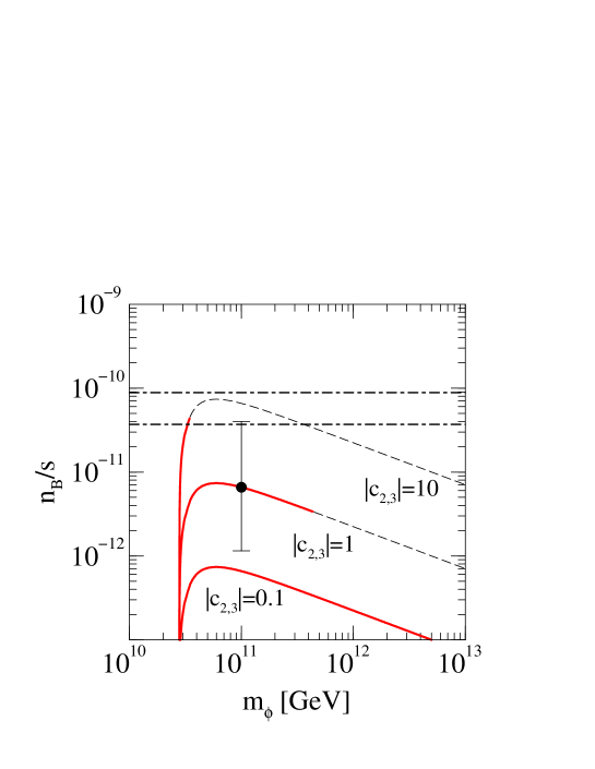
Figure 1: The produced baryon asymmetries $n_{B}/s$ are shown by the (red) thick-solid lines for $\left|c_{2,3}\right|=0.1,1$ and $10$, respectively. The dashed lines represent the regions where the reheating temperature is higher than the lightest Majorana mass $T_{R}>M_{1}$. The typical effect of the statistical error of the $CP$ asymmetries $\epsilon_{2,3}$ is also represented for $m_{\phi}=1\times 10^{11}~{}\mbox{\rm GeV}$ and $\left|c_{2,3}\right|=1$. The observed $n_{B}/s$ are denoted by the region between the horizontal dot-dashed lines.

In Figure 1 we show the produced baryon asymmetries (63) by using the exact formula for the inflaton decay width in Eq. (70). We neglect the region where the reheating temperature is higher than the lightest Majorana neutrino mass $T_{R}>M_{1}$. It can be seen that the observed baryon asymmetry is obtained when the inflaton mass is close to $2M_{2,3}$ with $\left|c_{2,3}\right|\sim 10$. The inflaton mass of $m_{\phi}\sim 2M_{2,3}$ but $m_{\phi}>2M_{2,3}$ is crucial to have a sufficiently low reheating temperature $T_{R}\,\raisebox{-2.58334pt}{${\textstyle\stackrel{{\scriptstyle<}}{{\sim}}}$}\,M_{1}$ in order to avoid the wash-out of the produced asymmetry by $N_{1}$, as well as to have a larger baryon asymmetry.

One might worry that we only get agreement with the baryon asymmetry for the value $10$ of the order one constants, $c_{2}=c_{3}=10$, given in Eq. (69). However, it is basically not a problem at all: we have used the best fitted values for the $CP$-asymmetry parameters $\epsilon_{2,3}$, but they have large statistical uncertainty as represented in Eq. (3.4). We show this typical error also in Figure 1. It is found that the observed baryon asymmetry is easily obtained with $\left|c_{2,3}\right|\sim$ a few, which is very consistent with the philosophy that every dimensionless coupling takes an order one value at the fundamental scale.

To summarize, we have found that the proposed non-thermal scenario for the leptogenesis indeed works well in the family replicated gauge group model, and the dominant contributions to the present baryon asymmetry comes from the out-of-equilibrium decays of the heavier Majorana neutrinos $N_{2}$ and $N_{3}$ rather than the lightest one, $N_{1}$. To avoid the strong wash-out of the produced lepton asymmetry mediated by $N_{1}$, it is crucial that the inflaton decays into $N_{2}$ and $N_{3}$ at the late time via the interaction terms in Eq. (69), which ensures naturally the reheating temperature of sufficiently low. Interesting enough, we have observed that the successful baryogenesis requires (or predicts) the mass of the inflaton of $m_{\phi}\sim 2M_{2,3}\sim 10^{10}~{}\mbox{\rm GeV}$.

5 Discussion

5.1 Problem of decay into Weinberg-Salam Higgs particles

For the successful baryogenesis the inflaton particle should survive until the era of the temperature $T\raisebox{-2.58334pt}{${\textstyle\stackrel{{\scriptstyle<}}{{\sim}}}$}M_{1}$, when the “accidental” conservation law of the $B-L$ charge has been installed to prevent the wash-out of the produced lepton asymmetry. Furthermore, the branching ratio of the inflaton decays into the heavier Majorana neutrinos $N_{2}$ and $N_{3}$ should be sufficiently large to account for the observed baryon asymmetry. To realize this long-lived inflaton it is crucial that the total decay width of the inflaton $\Gamma_{\phi}$ is really dominated by the decays into the Majorana neutrinos $N_{2}$ and $N_{3}$ via the interaction (69).

In the family replicated gauge group model discussed above, other inflaton decay channels than the Majorana neutrinos do exist. In fact, the inflaton can also decay into pairs of quarks or charged leptons. These decay amplitudes are proportional to the masses of the produced fermions, and hence it is naturally understandable that the heaviest fermions ${N_{2}}$ and $N_{3}$ will dominate among the final states of two fermions. Moreover, by assuming the philosophy that the dimensionless couplings are of order one, we naturally expect that the Higgs fields in the considered model obtain the masses of order of their VEVs. Among these the Higgs fields, the masses of $W$, $T$, $\rho$, $\omega$, and $\phi_{\scriptscriptstyle\rm SS}$ are sufficiently heavy (see Eq. (3.4)) that the inflaton of mass $m_{\phi}\sim 2M_{2,3}$ cannot kinematically decay into them. The inflaton also decays into pairs of gauge bosons in the Standard Model, i.e., photons, $W^{\pm}$-bosons, $Z^{0}$-bosons, and gluons. These decay channels would be potentially dangerous depending on the inflaton mass. However, in the inflaton mass region we are interested in (i.e., $m_{\phi}\sim 2M_{2,3}$ but well above threshold) the partial widths of decays into the Standard Model gauge bosons are comparable to those of $\phi\rightarrow N_{2,3}N_{2,3}$. Therefore, they do not disturb our successful leptogenesis scenario. Other gauge fields appear in the considered model obtain the masses from the Higgs fields $W$, $T$, $\rho$, $\omega$, and $\phi_{\scriptscriptstyle\rm SS}$, and the inflaton decays into these gauge fields are kinematically forbidden.

However, there is one point that needs discussions: why should the inflaton not decay into a couple of Weinberg-Salam Higgs bosons, one Higgs and one anti-Higgs? A priori there could exist interaction terms in the Lagrangian density of the form

$${\cal L}=\mu~{}\phi~{}\left|\phi_{\rm\scriptscriptstyle WS}\right|^{2}\,+\lambda\,\phi^{2}\,\left|\phi_{\rm\scriptscriptstyle WS}\right|^{2}\,,$$ (72)

where $\mu$ is a mass parameter and $\lambda$ a coupling constant. These interactions allow the inflaton decay with a width

$$\Gamma(\phi\rightarrow\phi_{\rm\scriptscriptstyle WS}\,\phi_{\rm\scriptscriptstyle WS}^{\dagger})=\frac{1}{8\pi}\frac{\left(\mu+\lambda\left\langle\phi\right\rangle\right)^{2}}{m_{\phi}}~{}.$$ (73)

That would, however, have the adverse effect of allowing the fast decay of the inflaton and making the formal reheating temperature $T_{R}$ in Eq. (2) higher than the mass of $\phi$, $m_{\phi}$, since we expect from our philosophy the coupling $\lambda$ be the order unity and also the inflaton and its VEV be of the same order, $m_{\phi}\sim\left\langle\phi\right\rangle$. It means that the $\phi$ inflaton would decay immediately after the inflation, with exceedingly small branching rations to seesaw neutrinos and our picture would be spoiled. In practice, in order that the $\phi_{\rm\scriptscriptstyle WS}\,\phi_{\rm\scriptscriptstyle WS}^{\dagger}$-channel leave the Majorana neutrino channel(s) to dominate, the required suppression of the effective coupling $\lambda_{\rm\scriptscriptstyle eff}$ compared to unity is found from Eqs. (70) and (73) to be of the order of

$$\lambda_{\rm\scriptscriptstyle eff}=\lambda+\frac{\mu}{\left\langle\phi\right\rangle} \ll \left|c_{2,3}\right|\frac{m_{\phi}}{\left\langle\phi\right\rangle}\,\frac{M_{2,3}}{M_{\ast}}$$ (74)

$$\approx \left|c_{2,3}\right|\frac{M_{2,3}}{M_{\ast}}\approx 10^{-8}\cdot\left|c_{2,3}\right|\left(\frac{M_{2,3}}{10^{10}~{}\mbox{\rm GeV}}\right)\hskip 5.69054pt,$$

where we assumed that the mass of the inflaton and its VEV are of the same order, $m_{\phi}/\left\langle\phi\right\rangle\approx 1$. Therefore, to realize the successful leptogenesis the coefficients $\lambda$ and $\mu/\left\langle\phi\right\rangle$ should be extremely small contrary to our basic philosophy. This is a drawback of the proposed scenario.

However, first of all, we must say that we had already accepted this kind of finetuning of parameters in the model. Since we have no symmetry to control radiative corrections, we would expect every mass parameter in the model to be of the order of the fundamental cutoff scale, e.g., the Planck mass, under the assumption of dimensionless coupling being order unity. On the contrary, we had already introduced the mass scales which is smaller than the Planck scale, which are the VEVs (or masses) of the Higgs fields. The most severe one is the mass of the Weinberg-Salam Higgs. Although the hierarchy in various Yukawa couplings to explain the observed mass spectrum of fermions can be very elegantly explained by the flavor (gauge) symmetry, we had not explained the hierarchy between the Planck scale and the mass scales of interest, but just realized it by finetuning by hand. In fact, as an example, the order unity coupling $\lambda_{\rm\scriptscriptstyle eff}={\cal O}(1)$ also induces the huge correction to the mass of the Weinberg-Salam Higgs particle, i.e., $\delta m_{\rm\scriptscriptstyle WS}=\sqrt{\lambda_{\rm\scriptscriptstyle eff}}\left\langle\phi\right\rangle\sim\sqrt{\lambda_{\rm\scriptscriptstyle eff}}\,m_{\phi}\sim 10^{10}~{}\mbox{\rm GeV}$. To have the weak scale mass $\sim 10^{2}~{}\mbox{\rm GeV}$ for the Weinberg-Salam Higgs, the coupling would be extremely small $\lambda_{\rm\scriptscriptstyle eff}\ll 10^{-16}$, which is more stringent than Eq. (74). However, this is not a matter at all from our standpoint, since, in addition to other dangerous (radiative) corrections, such a huge contribution is tremendously tuned so as to have the Weinberg-Salam Higgs mass of the weak scale $\sim 100~{}\mbox{\rm GeV}$. In the considered model we had already accepted the finetuning for the mass parameters in the scalar sector. Therefore, the required suppression of the coefficients as given in Eq. (74), which makes the non-thermal leptogenesis works well, is a problem of our attitude toward the finetuning. Although we loose the simple philosophy of couplings being order unity, the successful leptogenesis might be obtained just by accepting not only the finetuning for the hierarchy problem, but also of the dimensionless couplings appearing in the scalar sector. Moreover, it should be remarked that inflaton scheme in general suffers from difficulties to allow the inflaton interactions with the Standard Model particles for the reheating, since the interactions should be sufficiently weak not to spoil the slow-roll inflation scenario.

Although the required suppression in Eq. (74) would be easily achieved by the finetuning, hereafter we will briefly discuss two possible resolutions of the finetuning problems.

5.1.1 Multiple point principle “explanation” of suppression of inflaton decay to Weinberg-Salam Higgses

One possible attempt to explain the absence of the terms, e.g., $\lambda\,\left|\phi_{\rm\scriptscriptstyle WS}\right|^{2}\,\phi^{2}$ term consists in calling upon a principle which has actually been developed in connection with the model discussed here as the example. This is the postulate of the multiple point principle (MPP) [24], saying that the effective potential as a function of the scalars such as $\phi_{\scriptscriptstyle\rm WS}$ and $\phi$ $\hbox{\it etc}{}.$ should have many (as many as possible) equally deep minima. This is a principle that is actually true in superdsymmetric models in as far as there all the superdsymmetric states have to have zero and (thus) minimal energy density.

In the article [25] it was argued that such a principle of equally deep minima would have a tendency to split into separate sectors – totally decoupling ones – once there are only one (or a few) free parameters adjustable interactions between potentially separable sectors.

Ignoring the irrelevant terms such as Eq. (69) the only interaction between an “inflation sector” and “our sector” – meaning the Standard Model fields plus the seesaw neutrinos as well as possible gauge fields or scalars associated with it – is supposed to be the term $\lambda\,\left|\phi_{\rm\scriptscriptstyle WS}\right|^{2}\,\left|\phi\right|^{2}$ in Eq. (72).

Now we want to argue that provided we could find solutions for the coupling constants with, say, two degenerate minima in both of the mentioned sectors, when they were separate, we can argue for that $\lambda=0$ is at least one possible solution for satisfying the MPP requirement. Let us argue for that by counting relations ($\approx$ finetunings) between the coupling constants needed to achieve degenerate minima in effective potentials: to achieve $n$ degenerate minima in an effective potential $V_{\rm eff}$ – it be a function of one or more scalar fields – one needs to finetune $(n-1)$ couplings or parameters. Let us for example imagine that if we had our sector alone MPP could tune in $2-1=1$ relation between the couplings and thereby achieve $2$ degenerate minima (in the Weinberg-Salam Higgs effective potential) and that one also by tuning $2-1=1$ coupling/parameter can achieve two generate minima in the inflaton effective potential, if that were alone. Then we can see easily that by combining the two sets of coupling constants and taking further $\lambda=0$, we achieve $4=2\cdot 2$ degenerate minima for the effective potential of the full model. This effective potential is (at least) a function of both $\phi$ and $\phi_{\rm\scriptscriptstyle WS}$ and it has its degenerate minima in all the $(\phi,\,\phi_{\rm\scriptscriptstyle WS})$-pairs which are obtained by combining the $\phi$-values from the degenerate minima in the $\phi$-potential alone and the $\phi_{\rm\scriptscriptstyle WS}$-values from the generate minima of “our sector” alone. There are $2\cdot 2=4$ such combinations $(\phi,\,\phi_{\rm\scriptscriptstyle WS})$ and thus this special solution with $\lambda=0$ provides $4$ degenerate minima. A priori we expect that $4$ degenerate minima requires $4-1=3$ finetuning relations between the couplings/parameters. The proposed solution with $\lambda=0$ uses just $3$ finetunings in as far as we used one finetuning relations for each of the two sectors plus the finetuning $\lambda=0$. The proposed solution has therefore not used more finetunings to be fixed by MPP than what is expected to be needed anyway. Had we instead imagined that we had got arranged say $3$ degenerate minima in the two sectors separately we would have been able to produce a solution with $\lambda=0$ and $9$ generate minima, that would have needed only $2+2+1=5$ finetunings against the a priori expected $9-1=8$ in this case. So in this case we would quite clearly get $\lambda=0$. We see here the possibility for the MPP to produce decoupling (totally) of only loosely coupled sectors, such as the inflaton one and ours.

The region in field space in which this kind of argument fixes $\lambda$ conceived of as renormalization group running with the fields $(\phi,\,\phi_{\rm\scriptscriptstyle WS})$ is of course where $\left|\phi\right|^{2}\,\left|\phi_{\rm\scriptscriptstyle WS}\right|^{2}$ is large. So a priori one may wonder if the running of $\lambda$ could let it be non-zero for some other field values. It is, however, rather easily seen that the $\beta$-function for $\lambda$ only obtain terms proportional to $\lambda$ itself. Thus once zero the coupling $\lambda$ will remain zero under the running.

5.1.2 Supersymmetric Extension

One of the most natural ways to explain the huge mass hierarchy between the fundamental Planck scale and the electroweak scale is to introduce an additional symmetry, supersymmetry (SUSY). It can stabilize the electroweak scale against the dangerous radiative corrections. Here we briefly discuss the SUSY extension of the family gauge replicated model and also its non-thermal leptogenesis.

In the family gauge replicated model with SUSY, we have to introduce two Weinberg-Salam Higgs (chiral super) fields, say $\phi_{u\rm\scriptscriptstyle WS}$ and $\phi_{d\rm\scriptscriptstyle WS}$, in order give masses to both the up-type quarks and the down-type quarks, respectively. Further, to ensure the cancellation of gauge and mixed anomalies, we introduce mirror (chiral super) fields of our Higgses, say, $W^{\prime}$, $T^{\prime}$, $\rho^{\prime}$, $\omega^{\prime}$, and $\phi_{\rm\scriptscriptstyle SS}^{\prime}$, for which the gauge charges are as if they were complex conjugates of $W$, $T$, $\rho$, $\omega$ and $\phi_{\rm\scriptscriptstyle SS}$. Then, in the SUSY models, the number of the (chiral super) fields for Higgs becomes doubled.

The first question we would like to ask is: “Can we reproduce the successful fitting of the masses and mixing for fermions which we performed in section 3?”. The answer is yes, to the first approximation. From the gauge invariance (i.e., six $U(1)$’s) we can write down the fermion mass matrices as Eqs. (17), (21), (25) and (29) by replacing $\left\langle\phi_{\rm\scriptscriptstyle WS}\right\rangle\to\left\langle\phi_{d\rm\scriptscriptstyle WS}\right\rangle$ and $\left\langle\phi_{\rm\scriptscriptstyle WS}^{\dagger}\right\rangle\to\left\langle\phi_{u\rm\scriptscriptstyle WS}\right\rangle$, and also by replacing the dagger Higgs fields to the mirror (chiral super) fields, e.g., $W^{\dagger}\to W^{\prime}$, as we must do since the superpotential shall be holomorphic. If we take $\left\langle\phi_{u\rm\scriptscriptstyle WS}\right\rangle=\left\langle\phi_{d\rm\scriptscriptstyle WS}\right\rangle$, the overall scale of the Dirac matrices is the same for the up-quarks, down-quarks, charged-leptons, and Dirac neutrinos, but is suppressed by $1/\sqrt{2}$ comparing with the non-SUSY model which is outside of our discussion. Furthermore, from the $D$-term flatness conditions, we expect that the VEVs of our Higgs fields are the same as those of mirror fields, e.g., $\left\langle W\right\rangle=\left\langle W^{\prime}\right\rangle$. It should thus be noted that in this use we have only the five VEVs $\left\langle W\right\rangle=\left\langle W^{\prime}\right\rangle$, $\left\langle T\right\rangle=\left\langle T^{\prime}\right\rangle$, $\left\langle\rho\right\rangle=\left\langle\rho^{\prime}\right\rangle$, $\left\langle\omega\right\rangle=\left\langle\omega^{\prime}\right\rangle$ and $\left\langle\phi_{\rm\scriptscriptstyle SS}\right\rangle=\left\langle\phi^{\prime}_{\rm\scriptscriptstyle SS}\right\rangle$ for the fitting even though we had introduced the doubled Higgs fields in the model compared with the non-SUSY model. Therefore, the structure of the Dirac and Majorana mass matrices remains unchanged at the cutoff scale, taken as the Planck scale. If we neglect the effects of the evolution by the renormalization group equation, we obtain the similar results given in Table $2$. Therefore, to the first approximation, we could say that we keep the successful fitting of masses and mixings even with SUSY introduced into the model.

The non-thermal leptogenesis is found to work in the SUSY version. By introducing SUSY, the total decay rate of the inflaton $\Gamma_{\phi}$ through the interaction Eq. (69), the decay rate asymmetry parameters of Majorana neutrinos $\epsilon_{i}$, and the degree of freedom of the thermal bath of the universe change only within a factor two which is also out of our discussion. Then, the inflaton of mass $m_{\phi}\sim 2M_{2,3}$ induce the reheating temperature of $T_{R}\sim 10^{6}\mbox{\rm GeV}$ and hence the correct order of baryon asymmetry is produced via the proposed scheme. Interestingly, with such low reheating temperatures we can avoid the cosmological gravitino problem [26].

Finally, we would like to ask; “Can we suppress the interactions between the Weinberg-Salam Higgs fields and the inflaton?”. The potentially dangerous interactions would be induced from the term in the superpotential as ${\cal W}=\phi\phi_{u\rm\scriptscriptstyle WS}\phi_{d\rm\scriptscriptstyle WS}$. This term can be killed by using the chiral $U(1)_{R}$ symmetry and the global $U(1)_{X}$ symmetry. We assign the $R$-charges $0$ for the Higgs fields and the inflaton, and $1$ for the matter fields. On the other hand, we assign the $X$-charges $0$ for our Higgs fields ($W$, $T$, $\rho$ and $\omega$) and the inflaton, $-2x$ for two Weinberg-Salam Higgs fields and the seesaw Higgs, and $x$ for the quark and lepton fields ($x$ is the charge corresponding to $U(1)_{X}$). This symmetry forbids ${\cal W}=\phi\phi_{u\rm\scriptscriptstyle WS}\phi_{d\rm\scriptscriptstyle WS}$ as well as the $\mu$-term ${\cal W}=\mu\phi_{u\rm\scriptscriptstyle WS}\phi_{d\rm\scriptscriptstyle WS}$. The required $\mu$-term may be generated by the effect of the SUSY breaking. Therefore, we can avoid the fast decay of the inflaton into the Weinberg-Higgs fields. Notice that the dangerous proton decay induced by the dimension five operator is also absent due to this $U(1)_{R}$ symmetry.

As we had briefly sketched, in the family replicated gauge group with SUSY, we have, to the first approximation, the successful fitting of masses and mixings for fermions as well as the non-thermal leptogenesis via heavier Majorana neutrinos produced by the late decays of the inflatons.

5.2 Further generalization, abstracting the model

It should be remarked that the idea of how to get the heavier seesaw neutrinos produced non-thermally in decay of an inflation boson, could be generalized to letting the boson – replacing the $\phi$ boson above – be any sufficiently long lived boson at the end decaying dominantly into the (heavier) seesaw neutrinos. Then it is possible that at the stage of the cosmological development when the temperature passes the mass $m_{\phi}$ of these particles, they become non-relativistic and we obtain a matter dominated era. Such an era will end when Hubble expansion rate, $H$, becomes of the order of the width $\Gamma_{\phi}$ by the decay of these particles – pretty analogous to the “reheating” talked about above.

That it is a true inflaton does not really matter, we could get by the same calculation as we did the same leptogenesis anyway. In this way we could escape completely mass estimates suggested for the inflaton. However, since the inflaton mass is very strongly dependent on the form of the inflation effective potential used, there is really no general mass estimation for the inflaton (in a model independent way). Therefore, it was correct that we used the mass for fitting $m_{\phi}{}\sim{}2M_{2,3}{}\sim 10^{10}~{}\mbox{\rm GeV}$.

6 Conclusions

In this article the leptogenesis by the decays of the heavier Majorana neutrinos $N_{2}$ and $N_{3}$ was considered. We pointed out that the $N_{2}$ and $N_{3}$ decays could be responsible for generating the baryon asymmetry in the present Universe, if they are produced non-thermally in the inflaton decays. In our picture then the reheating temperature of the inflation is sufficiently low that the wash-out processes mediated by the lighter Majorana neutrino are ineffective.

Accepting this picture for baryogenesis would release the family replicated gauge group model from its only severe deviation from agreement with experiment – the amount of baryon minus lepton number produced in the seesaw era – and thus make it agree within its pretended only order of magnitude accuracy with all quantities it predicts.

This means that with the combined picture of an inflaton as suggested here and the family replicated gauge group model – in the latest version – we have a very viable model where we used the five parameters to produce the fit of Table $2$ and some adjustment of the inflation properties essentially all the parameters useful for going beyond the Standard Model, however, only order of magnitudewise. Indeed we have now fit all the quark and lepton masses and mixings – including the neutrinos and the $CP$ violation – and the baryon asymmetry, and further successfully coped with bounds on proton decay and lepton flavor violating decays. Also bounds on the neutrinoless beta decay are respected though so that neither the positive findings of the Heidelberg-Moscow collaboration of $\left\langle\left|m_{ee}\right|\right\rangle\approx 0.39~{}\mbox{\rm eV}$ [23] nor the LSND neutrino [27] are welcome in our scheme.

References

- [1] D. E. Groom et al. [Particle Data Group Collaboration], Eur. Phys. J. C 15 (2000) 1.
- [2] M. Fukugita and T. Yanagida, Phys. Lett. B 174 (1986) 45.
-
[3]
T. Yanagida, in Proceedings of the Workshop on Unified
Theories and Baryon Number in the Universe, Tsukuba, Japan (1979), eds.
O. Sawada and A. Sugamoto, KEK Report No. 79-18;
M. Gell-Mann, P. Ramond and R. Slansky, in Supergravity, Proceedings of the Workshop at Stony Brook, NY (1979), eds. P. van Nieuwenhuizen and D. Freedman (North-Holland, Amsterdam, 1979). -
[4]
F. Wilczek, in Proceedings of the 9th International Symposium
on Lepton and Photon Interactions at High Energies, Batavia, Illinois, USA,
23-29 August, 1979, eds. T. B. W. Kirk and H. D. I. Abarbanel;
E. Witten, Phys. Lett. B 91 (1980) 81;
R. N. Mohapatra and G. Senjanović, Phys. Rev. Lett. 44 (1980) 912. - [5] V. A. Kuzmin, V. A. Rubakov and M. E. Shaposhnikov, Phys. Lett. B 155 (1985) 36.
- [6] For a review and references, see: W. Buchmüller and M. Plümacher, Int. J. Mod. Phys. A 15 (2000) 5047 [arXiv:hep-ph/0007176] and references therein.
-
[7]
G. Lazarides and Q. Shafi,
Phys. Lett. B 258, 305 (1991);
K. Kumekawa, T. Moroi and T. Yanagida, Prog. Theor. Phys. 92 (1994) 437 [arXiv:hep-ph/9405337];
G. Lazarides, Springer Tracts Mod. Phys. 163 (2000) 227 [arXiv:hep-ph/9904428] and references therin;
G. F. Giudice, M. Peloso, A. Riotto and I. Tkachev, JHEP 9908 (1999) 014 [arXiv:hep-ph/9905242];
T. Asaka, K. Hamaguchi, M. Kawasaki and T. Yanagida, Phys. Lett. B 464 (1999) 12 [arXiv:hep-ph/9906366]; Phys. Rev. D 61 (2000) 083512 [arXiv:hep-ph/9907559];
M. Kawasaki, M. Yamaguchi and T. Yanagida, Phys. Rev. D 63 (2001) 103514 [arXiv:hep-ph/0011104]. - [8] G. F. Giudice, M. Peloso, A. Riotto and I. Tkachev, in [7].
-
[9]
B. A. Campbell, S. Davidson and K. A. Olive, Nucl. Phys. B 399 (1993) 111 [arXiv:hep-ph/9302223];
H. Murayama and T. Yanagida, Phys. Lett. B 322 (1994) 349 [arXiv:hep-ph/9310297];
H. Murayama, H. Suzuki, T. Yanagida and J. Yokoyama, Phys. Rev. Lett. 70 (1993) 1912; Phys. Rev. D 50 (1994) 2356 [arXiv:hep-ph/9311326]. -
[10]
W. Buchmüller, arXiv:hep-ph/0204288;
W. Buchmüller, P. Di Bari and M. Plümacher, arXiv:hep-ph/0205349. - [11] H. B. Nielsen and Y. Takanishi, Nucl. Phys. B 588 (2000) 281 [arXiv:hep-ph/0004137]; Nucl. Phys. B 604 (2001) 405 [arXiv:hep-ph/0011062]; Phys. Scripta T93 (2001) 44 [arXiv:hep-ph/0101181]; Phys. Lett. B 507 (2001) 241 [arXiv:hep-ph/0101307]; C. D. Froggatt, H. B. Nielsen and Y. Takanishi, Nucl. Phys. B 631 (2002) 285 [arXiv:hep-ph/0201152]; H. B. Nielsen and Y. Takanishi, Nucl. Phys. B 636 (2002) 305 [arXiv:hep-ph/0204027].
- [12] H. B. Nielsen and Y. Takanishi, Phys. Lett. B 543 (2002) 249 [arXiv:hep-ph/0205180].
-
[13]
S. Y. Khlebnikov and M. E. Shaposhnikov, Nucl. Phys. B 308 (1988) 885;
J. A. Harvey and M. S. Turner, Phys. Rev. D 42 (1990) 3344. - [14] C. D. Froggatt and H. B. Nielsen, Nucl. Phys. B 147 (1979) 277.
- [15] M. B. Green and J. H. Schwarz, Phys. Lett. B 149 (1984) 117.
- [16] H. Arason, D. J. Castaño, B. Keszthelyi, S. Mikaelian, E. J. Piard, P. Ramond and B. D. Wright, Phys. Rev. D 46 (1992) 3945.
-
[17]
S. Antusch et al., Phys. Lett. B 519 (2001) 238
[arXiv:hep-ph/0108005];
P. H. Chankowski and P. Wasowicz, Eur. Phys. J. C 23 (2002) 249 [arXiv:hep-ph/0110237]. -
[18]
M. A. Luty, Phys. Rev. D 45 (1992) 455;
L. Covi, E. Roulet and F. Vissani, Phys. Lett. B384 (1996) 169 [arXiv:hep-ph/9605319];
W. Buchmüller and M. Plümacher, Phys. Lett. B431 (1998) 354 [arXiv:hep-ph/9710460]. - [19] C. D. Froggatt, H. B. Nielsen and D. J. Smith, Phys. Rev. D 65 (2002) 095007 [arXiv:hep-ph/0108262].
-
[20]
Q. R. Ahmad et al. [SNO Collaboration], Phys. Rev. Lett. 89 (2002) 011301 [arXiv:nucl-ex/0204008]; Phys. Rev. Lett. 89 (2002) 011302 [arXiv:nucl-ex/0204009];
S. Fukuda et al. [Super-Kamiokande Collaboration], Phys. Lett. B 539 (2002) 179 [arXiv:hep-ex/0205075]. - [21] M. B. Smy [Super-Kamiokande Collaboration], in the proceedings of 37th Rencontres de Moriond on Electroweak Interactions and Unified Theories, Les Arcs, France, 9-16 Mar 2002; arXiv:hep-ex/0206016.
- [22] C. Jarlskog, Phys. Rev. Lett. 55 (1985) 1039.
- [23] H. V. Klapdor-Kleingrothaus, A. Dietz, H. L. Harney and I. V. Krivosheina, Mod. Phys. Lett. A 16 (2001) 2409 [arXiv:hep-ph/0201231].
- [24] D. L. Bennett and H. B. Nielsen, Int. J. Mod. Phys. A 9 (1994) 5155 [arXiv:hep-ph/9311321]; Int. J. Mod. Phys. A 14 (1999) 3313 [arXiv:hep-ph/9607278].
- [25] C. D. Froggatt, H. B. Nielsen and Y. Takanishi, Phys. Rev. D 64 (2001) 113014 [arXiv:hep-ph/0104161].
-
[26]
M. Y. Khlopov and A. D. Linde,
Phys. Lett. B 138 (1984) 265;
J. R. Ellis, J. E. Kim and D. V. Nanopoulos, Phys. Lett. B 145 (1984) 181;
M. Kawasaki and T. Moroi, Prog. Theor. Phys. 93 (1995) 879 [arXiv:hep-ph/9403364]. - [27] C. Athanassopoulos et al. [LSND Collaboration], Phys. Rev. Lett. 77 (1996) 3082 [arXiv:nucl-ex/9605003]; Phys. Rev. C 58 (1998) 2489 [arXiv:nucl-ex/9706006]; Phys. Rev. Lett. 81 (1998) 1774 [arXiv:nucl-ex/9709006].