CERN-TH/2002-145

hep-ph/0207020

July 2002

Analytic Continuation of
Massless Two-Loop Four-Point Functions
T. Gehrmann^a and E. Remiddi^b
a Theory Division, CERN, CH-1211 Geneva 23, Switzerland
^b Dipartimento di Fisica, Università di Bologna and INFN, Sezione di Bologna, I-40126 Bologna, Italy

We describe the analytic continuation of two-loop four-point functions with one off-shell external leg and internal massless propagators from the Euclidean region of space-like $1\to 3$ decay to Minkowskian regions relevant to all $1\to 3$ and $2\to 2$ reactions with one space-like or time-like off-shell external leg. Our results can be used to derive two-loop master integrals and unrenormalized matrix elements for hadronic vector-boson-plus-jet production and deep inelastic two-plus-one-jet production, from results previously obtained for three-jet production in electron–positron annihilation.

1 Introduction

In recent years, considerable progress has been made towards the extension of QCD calculations of jet observables towards the next-to-next-to-leading order (NNLO) in perturbation theory. One of the main ingredients in such calculations are the two-loop virtual corrections to the multi leg matrix elements relevant to jet physics, which describe either $1\to 3$ decay or $2\to 2$ scattering reactions: two-loop four-point functions with massless internal propagators and up to one off-shell external leg.

Using dimensional regularization [1, 2] with $d\neq 4$ dimensions as regulator for ultraviolet and infrared divergences, the large number of different integrals appearing in the two-loop Feynman amplitudes for $2\to 2$ scattering or $1\to 3$ decay processes can be reduced to a small number of master integrals. The techniques used in these reductions are integration-by-parts identities [2, 3] and Lorentz invariance [4]. A computer algorithm for the automatic reduction of all two-loop four-point integrals was described in [4].

The use of these techniques allowed the calculation of two-loop QED and QCD corrections to many $2\to 2$ scattering processes with massless on-shell external particles [5], which require master integrals corresponding to massless four-point functions with all legs on-shell [6, 7]. The results in [5] are given for all three physical Mandelstam channels, which are related by analytic continuation. In [8], the full set of two-loop four-point master integrals with one external leg off-shell was computed, for the kinematical situation of a $1\to 3$ decay, by solving the differential equations in external invariants [4] fulfilled by these master integrals. These integrals were employed in the calculation of the two-loop QCD corrections to the $e^{+}e^{-}\to 3$ jets matrix element and to the corresponding helicity amplitudes in [9], which can be expressed as a linear combination (with rational coefficients in the invariants and the space-time dimension $d$) of the corresponding master integrals. The $2\to 2$ scattering processes related to $e^{+}e^{-}\to 3$ jets by analytic continuation and crossing are both of high phenomenological importance: hadronic vector-boson-plus-jet production and deep inelastic two-plus-one-jet production.

The two-loop four-point functions with all legs on-shell can be expressed in terms of Nielsen’s polylogarithms [10], which have a well-defined analytic continuation [10, 11]. The continuation of the master integrals in the on-shell case [6, 7] was discussed in detail in [7]. In contrast, the closed analytic expressions for two-loop four-point functions [8] with one leg off-shell contain two new classes of functions: harmonic polylogarithms (HPLs) [12, 13] and two-dimensional harmonic polylogarithms (2dHPLs) [14]. Accurate numerical implementations for HPLs [13] and 2dHPLs [14] are available. The implementations apply to HPLs of arbitrary real arguments [12, 13], but only for a limited range of arguments of the 2dHPLs. This range of arguments corresponds precisely to the Euclidean region (space-like $1\to 3$ decay) for the corresponding off-shell master integrals [8]. Continuation from the Euclidean region to any physical (Minkowskian) region requires in general the analytic continuation of the 2dHPLs outside the range of arguments considered in  [14]. Only in the special case of a time-like $1\to 3$ decay (relevant to $e^{+}e^{-}\to 3$ jets), which corresponds to the simultaneous continuation of all three external invariants from Euclidean to Minkowskian values, this continuation can be carried out by simply replacing an overall scaling factor, while preserving all 2dHPLs (which depend only on dimensionless ratios of the invariants). These results were used in [9] for the calculation of the two-loop matrix elements for $e^{+}e^{-}\to 3$ jets.

It is the aim of the present paper to derive the relations for HPLs and 2dHPLs needed for the analytic continuation of the two-loop four-point master integrals of [8] to the kinematics of all the $2\to 2$ scattering reactions with one off-shell external leg, working out real and imaginary parts explicitly. We also provide the algorithms for expressing them in terms of HPLs and 2dHPLs whose arguments lie within the range covered by the numerical routine of [14], which allows them to be evaluated numerically. Given that the matrix elements are linear combinations of the master integrals, this will in turn allow us to determine the matrix element for all $2\to 2$ reactions related to $e^{+}e^{-}\to 3$ jets by crossing.

In the context of the next-to-leading order (NLO) corrections to jet observables, the first calculation [15] was also for the kinematics of the $1\to 3$ decay, relevant to $e^{+}e^{-}\to 3$ jets. The one-loop matrix element obtained in this calculation contained only logarithms and dilogarithms, which have a known analytic continuation. The results of [15] were continued to the kinematic situation relevant to hadronic vector-boson-plus-jet production in [16], and to deep inelastic two-plus-one-jet production in [17, 18]. The analytic continuation procedure used in these calculations is documented in detail in [18]. In particular it is already observed at the one-loop level that the kinematic region relevant to the hadronic vector-boson-plus-jet production is free of kinematic cuts, while two kinematic cuts are present inside the region of deep inelastic two-plus-one-jet production. We shall see below that the same pattern is preserved at the two-loop level.

The paper is structured as follows. In Section 2, we define the kinematical variables used to describe two-loop four-point functions with one off-shell leg and describe the ranges of variables relevant to each different process by making a detailed decomposition of the kinematic plane. The basic features of analytic continuation are discussed in Section 3 on the example of the continuation of the $1\to 3$ decay from the Euclidean to the Minkowskian region. In Sections 4 and 5, we derive the algorithms for the analytic continuation in one invariant for a time-like and a space-like off-shell leg. Section 6 contains conclusions and an outlook. Finally, the Appendix recalls definitions and main properties of the HPLs and 2dHPLs.

2 Kinematic regions and notation

We label the external momenta on the four-point functions with $p_{1}$, $p_{2}$, $p_{3}$ and $p_{4}$, and write momentum conservation as $p_{1}+p_{2}+p_{3}+p_{4}=0\ ,$ with on-shell conditions $p_{i}^{2}=0$ for $i=1,2,3$ while $p_{4}$ is off-shell $p_{4}^{2}=(-p_{1}-p_{2}-p_{3})^{2}=q^{2}\neq 0$. We further define

$$s_{12}=(p_{1}+p_{2})^{2}\;,\quad s_{13}=(p_{1}+p_{3})^{2}\;,\quad s_{23}=(p_{2}+p_{3})^{2}\;,$$ (2.1)

so that the Mandelstam relation reads

$$s_{12}+s_{13}+s_{23}=q^{2}\ .$$ (2.2)

We will use the metric in which time-like invariants are positive. The kinematic plane defined by $s_{12}$, $s_{13}$ and $s_{23}$ is shown in Fig. 1, where equilateral (non-Cartesian) coordinates were used to display the symmetry in the three invariants. The lines indicate the locations of potential cuts in the four-point functions. For later use, all regions defined by these cuts are labelled as (1a), (1b), $\ldots$, (4d).

Figure 1: Kinematic plane in terms of Lorentz invariants $s_{ij}=(p_{i}+p_{j})^{2}$ displayed in equilateral coordinates.

The regions physically relevant to different processes are displayed in Fig. 2. In $e^{+}e^{-}\to 3$ jet ($3j$) production, $q^{2}$ is time-like (hence positive) and all $s_{ij}$ are positive as well. The relevant region is the inner triangle of the kinematic plane, as shown in Fig. 2(a). This inner triangle corresponds to region (1a) in Fig. 1. To indicate space-like ($q^{2}<0$) and time-like ($q^{2}>0$) kinematics for a region under discussion, we will use in the following the subscripts “$-$” (space-like) and “$+$” (time-like). The region relevant to $3j$-production is thus denoted by (1a)₊.

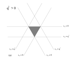
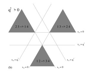
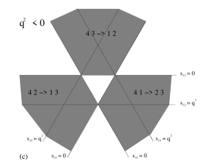
Figure 2: Regions of the kinematic plane relevant to (a) $e^{+}e^{-}\to 3$ jets $(q^{2}>0)$, (b) $(V+1)$ jet production $(q^{2}>0)$ and (c) deep inelastic $(2+1)$ jet production $(q^{2}<0)$.

Vector-boson-plus-jet ($V+1j$) production at hadron colliders and deep-inelastic two-plus-one-jet (DIS-$(2+1)j$) production are described by three subprocesses each (corresponding to the $s_{12},s_{13},s_{23}$ channels, which all contribute to these final states).

For $V+1j$ production, $q^{2}$ is time-like, and for $p_{i}+p_{j}\to p_{k}+p_{4}$ the invariants fulfil

$$q^{2}>0\;,\quad s_{ij}>q^{2}>0\;,\quad s_{jk}<0\;,\quad s_{ik}<0\;,$$ (2.3)

where $(i,j,k)$ stand for the three non-ordered permutations of $(1,2,3)$. The relevant regions are shown in Fig. 2(b) and correspond to the regions (2a,3a,4a)₊ of the kinematic plane, Fig. 1.

Finally, for DIS-$(2+1)j$ production, $q^{2}$ is space-like (hence negative) and for $p_{4}+p_{k}\to p_{i}+p_{j}$ the invariants fulfil

$$q^{2}<0\;,\quad s_{ij}>-q^{2}>0\;,\quad s_{jk}<0,\quad s_{ik}<0\;,$$ (2.4)

where $(i,j,k)$ stand again for the three non-ordered permutations of $(1,2,3)$. We display the relevant kinematic regions in Fig. 2(c). Each of those regions cannot be identified with a single region in the kinematic plane, Fig. 1, but is instead patched together from four regions, (1d,2c,3b,4d), (1b,2d,3c,4c) and (1c,2b,3d,4b).

Figure 3: Kinematic plane in Cartesian coordinates.

It is customary to introduce the dimensionless variables

$$x=\frac{s_{12}}{q^{2}}\;,\quad y=\frac{s_{13}}{q^{2}}\;,\quad z=\frac{s_{23}}{q^{2}}\;,$$ (2.5)

for which (2.2) reads

$$x+y+z=1\;.$$ (2.6)

As independent variables, we will use mainly $q^{2}$, $y$ and $z$, with $x$ therefore given as $x=1-y-z$. We will further represent the various kinematical configurations, at given $q^{2}$, in the Cartesian $y,z$ plane. For convenience of later use, we represent in Fig. 3 the whole $y,z$ plane properly partitioned in all the regions which will be of interest later. The labelling of the regions is as in Fig. 1.

When the three regions ($3j$, $V+1j$, DIS-$(2+1)j$), are superimposed, regardless of $q^{2}$, they cover the entire $(y,z)$ plane.

Despite using mainly $q^{2}$, $y$ and $z$ as independent variables, all analytic continuations are to be carried out in the original Mandelstam variables $s_{12}$, $s_{13}$ and $s_{23}$, adding to them, when time-like, the usual infinitesimal imaginary part with positive sign, $s_{ij}+i\epsilon$. Indeed, no definite sign can be attributed a priori to the imaginary parts of the dimensionless invariants $x$, $y$ and $z$, given the constraint $x+y+z=1$. In practice, this means that any function of $y$ and $z$ that is to be continued analytically, has to be expressed first in terms of $s_{12}$, $s_{13}$ and $s_{23}$, then continued taking correct account of the well defined imaginary parts of the $s_{ij}$, then finally re-expressed in $q^{2}$ and $y,z$ or other dimensionless variables appropriate to the considered region.

3 Basics of analytic continuation

The problem of analytic continuation is best discussed starting from the unphysical Euclidean case in which $q^{2},s_{12},s_{13}$ and $s_{23}$ are all space-like (hence negative). Let us give them the values

$$q^{2}=-Q^{2},\quad s_{ij}=-\sigma_{ij}$$ (3.1)

with

$$Q^{2}>0\;,\quad\sigma_{ij}>0\;,\quad\sigma_{12}+\sigma_{13}+\sigma_{23}=Q^{2}\;.$$ (3.2)

All master integrals are indeed real in this configuration. According to Eq. (2.5), we introduce

$$x=\frac{s_{12}}{q^{2}}=\frac{\sigma_{12}}{Q^{2}}\;,\quad y=\frac{s_{13}}{q^{2}}=\frac{\sigma_{13}}{Q^{2}}\;,\quad z=\frac{s_{23}}{q^{2}}=\frac{\sigma_{23}}{Q^{2}}\;,$$

and observe that, because of Eq. (3.2), we have $(0<y<1,\ 0<z<1-y)$ or equivalently $(0<z<1,\ 0<y<1-z)$, i.e. $(y,z)$ are in the region (1a) of Fig. 3. Any of the master integrals evaluated in [8], say $\Psi(s_{12},s_{13},s_{23})$, can be written as

$$\Psi(s_{12},s_{13},s_{23}) = (Q^{2})^{\alpha}\Phi\left(\frac{\sigma_{13}}{Q^{2}},\frac{\sigma_{23}}{Q^{2}}\right)$$ (3.3)

$$= (-q^{2})^{\alpha}\Phi\left(\frac{s_{13}}{q^{2}},\frac{s_{23}}{q^{2}}\right)$$

$$= (-q^{2})^{\alpha}\Phi(y,z)\ ,$$

where use is made of Eq. (3) and $\alpha$ is an exponent accounting for the mass dimension of the integral: $\alpha=d-r+s$, where $d$ is the continuous space-time dimension used in dimensional regularization, while the integers $r$ and $s$ denote the number of propagators and scalar products in the integral. For a two-loop seven-propagator master integral (e.g. a scalar double box or crossed box integral), with all propagators raised to unit power and no scalar products, one thus has $\alpha=d-7=-3+(d-4)$. The function $\Phi(y,z)$ is in general a Laurent series in $(d-4)$, whose coefficients are combinations of simple algebraic factors in $y,z$ times HPLs of various weight and argument $z$ and 2dHPLs of various weight and argument $y$, with indices depending on $z$.

Note that the dimensionless ratios $y,z$ are both real and positive, and lie within the boundaries $0<z<1$, $0<y<1-z$. In that range of values of the arguments, all the HPLs and 2dHPLs are analytic and real – as expected, of course, as all the kinematical variables are Euclidean. This region coincides with the triangle (1a)_- of Fig. 3.

As a consequence of the symmetry and analyticity properties of the HPLs and 2dHPLs, within the region (1a)_- we can exchange the roles of $y$ and $z$ and re-express the master integrals as

$$\Psi(s_{12},s_{13},s_{23})=(-q^{2})^{\alpha}\Phi^{\prime}(z,y)\ ,$$ (3.4)

where $\Phi^{\prime}(z,y)$ consists of HPLs of argument $y$ and 2dHPLs of argument $z$ with indices depending on $y$, all within their analyticity region. The transformation from $\Phi(y,z)$ to $\Phi^{\prime}(z,y)$ can be implemented, within the triangle (1a) of Fig. 3, by re-expressing the HPLs $\hbox{H}(\vec{m};z)$ and 2dHPLs $\hbox{G}(\vec{m}(z);y)$ as a combination of HPLs $\hbox{H}(\vec{m};y)$ and 2dHPLs $\hbox{G}(\vec{m}(y);z)$, by means of the ‘interchange-of-arguments’ procedure described in Appendix A.2.2 of [8]. All algorithms used for this procedure (and for all subsequent transformations derived in this paper) were coded in FORM [19].

Similarly, within the region (1a) we can replace $z=1-x-y$ by $x$, obtaining another representation of the master integrals

$$\Psi(s_{12},s_{13},s_{23})=(-q^{2})^{\alpha}\Phi^{\prime\prime}(y,x)\ ,$$ (3.5)

where $\Phi^{\prime\prime}(y,x)$ consists of HPLs of argument $x$ and 2dHPLs of argument $y$, with indices depending on $x$, all within their analyticity region. The above transformation, which amounts to re-expressing the HPLs $\hbox{H}(\vec{m};z)$ and 2dHPLs $\hbox{G}(\vec{m}(z);y)$ appearing in the original $\Phi(y,z)$ in terms of HPLs $\hbox{H}(\vec{n};x)$ and 2dHPLs $\hbox{G}(\vec{n}(x);y)$, with $x=1-y-z$, can be implemented as a result of the combination of the ‘interchange-of-arguments’-procedure described in Appendix A.2.2 of [8] with the reflection algorithm derived in Section 5 of [14].

The notation for the 2dHPLs used in the present work is shortly recalled in the Appendix. It is the same as was introduced in [14], which is however different from the notation originally proposed and used in [8] to present the two-loop four-point master integrals. The notation of [14] was already employed in [9] to represent the result for the two-loop QCD corrections to the $3j$ matrix element. Detailed transformation rules between the two notations can be found in [14]. A summary of definitions and properties of HPLs and 2dHPLs is provided in the appendix of [9].

In the $3j$ case, all the kinematical variables are time-like, hence positive; the proper analytic continuation is obtained by starting from the Euclidean case and giving to each positive variable (hence to all the variables in this case) a small positive imaginary part (the usual $+i\epsilon$ prescription). Equation (3.3) then becomes

$$\Psi(s_{12}+i\epsilon,s_{13}+i\epsilon,s_{23}+i\epsilon)=(-q^{2}-i\epsilon)^{\alpha}\Phi\left(\frac{s_{13}+i\epsilon}{q^{2}+i\epsilon},\frac{s_{23}+i\epsilon}{q^{2}+i\epsilon}\right).$$ (3.6)

The real parts of $(s_{13}+i\epsilon)/(q^{2}+i\epsilon)$ and $(s_{23}+i\epsilon)/(q^{2}+i\epsilon)$,

$$\frac{s_{13}}{q^{2}}=y\;,\quad\quad\frac{s_{23}}{q^{2}}=z\;,$$ (3.7)

lie in the region $0<y<1$, $0<z<1-y$, the triangle (1a) of Fig. 3, where all the HPLs and 2dHPLs are analytic and real. The $\epsilon\to 0$ limit is then trivial (i.e. the $i\epsilon$ can be simply ignored) and Eq. (3.6) becomes

$$\Psi(s_{12}+i\epsilon,s_{13}+i\epsilon,s_{23}+i\epsilon)=(-q^{2}-i\epsilon)^{\alpha}\Phi(y,z)\ ,$$ (3.8)

where $\Phi(y,z)$ is exactly the same as in the fully Euclidean case. The continuation from (1a)_- to (1a)₊ performed here leaves $\Phi(y,z)$ unchanged. The imaginary parts of the $3j$ master integrals (which are of course complex) are entirely due to the factor $(-q^{2}-i\epsilon)^{\alpha}$. The integer part of $\alpha$ does not matter, while the expansion in $(d-4)$ gives

$$(-q^{2}-i\epsilon)^{d-4}=1+(d-4)\bigl{(}\hbox{ln}(q^{2})-i\pi\bigr{)}+\frac{1}{2}(d-4)^{2}\bigl{(}\hbox{ln}(q^{2})-i\pi\bigr{)}^{2}+...\;.$$ (3.9)

It is worth recalling that the master integrals, as well as the physical matrix elements, develop polar singularities around $d=4$ in dimensional regularization, so that these higher-order terms in the $(d-4)$-expansion and their imaginary parts become of actual importance.

It is to be emphasised here that in [8], strictly speaking, the master integrals $\Psi(s_{12},s_{13},s_{23})$ were never directly evaluated in the fully Euclidean region; but as $\Phi(y,z)$ is the same function, and for the same range of arguments, in both the fully Euclidean case, Eq. (3.3), and the $3j$ case, Eq. (3.8), we can define in that way (i.e. by just replacing in the overall scale factor $(-q^{2}-i\epsilon)^{\alpha}$ by $(Q^{2})^{\alpha}$) the Euclidean master integrals in terms of the master integrals given in [8] for the $3j$ case. From now on, we will therefore take the Euclidean master integrals as known, and will show how to get by analytic continuation the master integrals in the various kinematical regions of physical interest.

4 Analytic continuation in one invariant for time-like $q^{2}$

To continue from region (1a)_- to regions (2a,3a,4a)₊, which are relevant to $V+1j$ production at hadron colliders (with a time-like momentum of the vector boson $V$), it is necessary to continue simultaneously in one of three Lorentz invariants $s_{ij}$ and in the vector boson virtuality $q^{2}$.

We start by discussing the continuation from (1a)_- to (4a)₊ .

In region (4a)₊ of Fig. 3, relevant for $V+1j$ production in the momentum arrangement $p_{2}+p_{3}\to p_{1}+p_{4}$, ($1<z<\infty,\ 1-z<y<0$) or ($-\infty<y<0,\ 1-y<z<\infty$) and

$$q^{2}>0,\ \ s_{12}<0,\ \ s_{13}<0,\ \ \ s_{23}=q^{2}-s_{12}-s_{13}>q^{2}>0\ ,$$ (4.1)

so that for the analytic continuation $q^{2}$ and $s_{23}$ must be given infinitesimal imaginary parts $+i\epsilon$. From Eq. (3.3) one gets in this case

$$\Psi(s_{12},s_{13},s_{23}+i\epsilon)=(-q^{2}-i\epsilon)^{\alpha}\Phi\left(\frac{s_{13}}{q^{2}+i\epsilon},\frac{s_{23}+i\epsilon}{q^{2}+i\epsilon}\right)=(-q^{2}-i\epsilon)^{\alpha}\Phi(y+i\epsilon,z-i\epsilon),$$ (4.2)

where, because of Eqs. (4.1) and of the very definition of $y,z$, Eqs. (2.5), we have used

$$\frac{s_{13}}{q^{2}+i\epsilon}=\frac{s_{13}}{q^{2}}+i\epsilon=y+i\epsilon\ ,\ \ \ \frac{s_{23}+i\epsilon}{q^{2}+i\epsilon}=\frac{s_{23}}{q^{2}}-i\epsilon=z-i\epsilon\ .$$ (4.3)

We introduce new dimensionless variables $u,v$ through the relations

$$u_{{\rm 4a}}=u=-\frac{s_{13}}{s_{23}}=-\frac{y}{z},\qquad v_{{\rm 4a}}=v=\frac{q^{2}}{s_{23}}=\frac{1}{z}\;,$$ (4.4)

so that

$$y=-\frac{u}{v}\ ,\ \ \ z=\frac{1}{v}\ .$$ (4.5)

As $y$ and $z$ span the region (4a) of Fig. 3, we find that $u,v$ vary in the ranges $0<v<1$ and $0<u<1-v$, i.e. the above parametrisation maps region (4a) into region (1a).

Equation (4.2) then reads

$$\Psi(s_{12},s_{13},s_{23}+i\epsilon)=(-q^{2}-i\epsilon)^{\alpha}\Phi\left(-\frac{u}{v}+i\epsilon,\frac{1}{v}-i\epsilon\right).$$ (4.6)

Given the above prescription, it is relatively straightforward to determine the proper analytic continuation of the various HPLs and 2dHPLs appearing in the analytic expression $\Phi(y,z)$ of any master integral and then to express them as HPLs of argument $v$ and 2dHPLs of argument $u$ and indices depending on $v$, with $(u,v)$, as already observed, within the analyticity triangle of the functions. Let us start from the HPLs and 2dHPLs of weight $w$ equal to 1, which are just logarithms. According to the definitions of the appendix, one has

$$\hbox{H}(0;z-i\epsilon) = \log\left(\frac{1}{v}-i\epsilon\right)=-\log{v}$$

$$= -\hbox{H}(0;v)\;,$$

$$\hbox{H}(1;z-i\epsilon) = -\log\left(1-\frac{1}{v}+i\epsilon\right)=-\log(1-v)+\log{v}-i\pi$$ (4.7)

$$= \hbox{H}(1;v)+\hbox{H}(0;v)-i\pi\;.$$

Notice that for $\hbox{H}(0;z)$, the $i\epsilon$-term can safely be ignored.

The 2dHPLs at $w=1$, again according to the definitions of the appendix, are continued as

$$\hbox{G}(0;y+i\epsilon) = \log\left(-\frac{u}{v}+i\epsilon\right)=\log\left(\frac{u}{v}\right)+i\pi$$

$$= \hbox{G}(0;u)-\hbox{H}(0;v)+i\pi$$

$$\hbox{G}(1;y+i\epsilon) = \log\left(1+\frac{u}{v}-i\epsilon\right)$$

$$= \hbox{G}(-v;u)$$

$$\hbox{G}(1-z+i\epsilon;y+i\epsilon) = \log\left(\frac{1+\frac{u}{v}-i\epsilon-\frac{1}{v}+i\epsilon}{1-\frac{1}{v}+i\epsilon}\right)=\log\left(\frac{1-u-v}{1-v}\right)$$

$$= \hbox{G}(1-v;u)$$

$$\hbox{G}(-z+i\epsilon;y+i\epsilon) = \log\left(\frac{-\frac{u}{v}+i\epsilon+\frac{1}{v}-i\epsilon}{\frac{1}{v}-i\epsilon}\right)=\log(1-u)$$ (4.8)

$$= \hbox{G}(1;u)\;.$$

It should be noted that no definite imaginary parts can be assigned to the arguments of the logarithms in $\hbox{G}(1-z+i\epsilon;y+i\epsilon)$ and $\hbox{G}(-z+i\epsilon;y+i\epsilon)$; but as the arguments in both cases remain positive and within the analyticity region of the functions, the result is anyhow well defined.

Using the above formulae, all imaginary parts of the higher weight HPLs and 2dHPLs are fixed, since these functions can be derived iteratively, starting from the $w=1$ functions, as will now be shown.

If, in an HPL of weight $w$ higher than $1$, all the indices are equal to $1$, that HPL is just equal to $1/w!$ times the $w$-th power of $\hbox{H}(1;z-i\epsilon)$, already seen. When the indices are not all equal to 1, one can first separate all leftmost $(1)$’s in the index vector, using the product algebra (A.9), such that the leftmost index is always a $(0)$. Any HPL can then be written as [13]

$$\hbox{H}(0,\vec{b};z-i\epsilon) = \hbox{H}(0,\vec{b};1-i\epsilon)+\int_{1-i\epsilon}^{z-i\epsilon}\hbox{d}z^{\prime}\frac{\hbox{d}}{\hbox{d}z^{\prime}}\hbox{H}(0,\vec{b};z^{\prime})$$ (4.9)

$$= \hbox{H}(0,\vec{b};1)+\int_{1}^{z}\hbox{d}z^{\prime}\frac{\hbox{d}}{\hbox{d}z^{\prime}}\hbox{H}(0,\vec{b};z^{\prime}-i\epsilon)$$

$$= \hbox{H}(0,\vec{b};1)-\int_{1}^{v}\frac{\hbox{d}v^{\prime}}{v^{\prime}}\hbox{H}\left(\vec{b};\frac{1}{v^{\prime}}-i\epsilon\right)\;,$$

where in the last step the integration variable $v^{\prime}=1/z^{\prime}$ was introduced. The expression for $\hbox{H}(\vec{b};1/v^{\prime}-i\epsilon)$ in terms of $\hbox{H}(\vec{c};v^{\prime})$ and its proper imaginary part is of lower weight than $\hbox{H}(0,\vec{b};z-i\epsilon)$ and thus already known in an iterative bottom up approach in the weight $w$. As an example of this transformation, one finds

$$\hbox{H}(0,1,1;z-i\epsilon) = \hbox{H}(0,0,1;v)-\hbox{H}(0,1,1;v)+\hbox{H}(0;v)\biggl{(}\frac{\pi^{2}}{2}-\hbox{H}(0,1;v)-\frac{1}{6}\hbox{H}(0;v)\hbox{H}(0;v)\biggr{)}+\zeta_{3}$$ (4.10)

$$-i\pi\biggl{(}-\hbox{H}(0,1;v)-\frac{1}{2}\hbox{H}(0;v)\hbox{H}(0;v)+\frac{\pi^{2}}{6}\biggr{)}\ .$$

To perform the analytic continuation of the 2dHPL in $y$, one first separates off all rightmost $(0)$’s in the index vector by applying the product algebra. The remaining 2dHPL (the dependence of the indices $a,\vec{b}$ on $z=1/v-i\epsilon$ is understood for short) can then be written as

$$\hbox{G}\left(a,\vec{b};-\frac{u}{v}+i\epsilon\right) = \int_{0}^{-\frac{u}{v}+i\epsilon}\hbox{d}y^{\prime}\frac{\hbox{d}}{\hbox{d}y^{\prime}}\hbox{G}(a,\vec{b};y^{\prime})$$ (4.11)

$$= \int_{0}^{-\frac{u}{v}}\hbox{d}y^{\prime}\frac{\hbox{d}}{\hbox{d}y^{\prime}}\hbox{G}(a,\vec{b};y^{\prime}+i\epsilon)$$

$$= \int_{0}^{-\frac{u}{v}}\hbox{d}y^{\prime}\hbox{g}(a,y^{\prime}+i\epsilon)\hbox{G}(\vec{b};y^{\prime}+i\epsilon)$$

$$= -\int_{0}^{u}\hbox{d}u^{\prime}\ \frac{1}{v}\hbox{g}\left(a,-\frac{u^{\prime}}{v}+i\epsilon\right)\,\hbox{G}\left(\vec{b};-\frac{u^{\prime}}{v}+i\epsilon\right),$$

where the expression for $\hbox{G}(\vec{b};-u^{\prime}/v+i\epsilon)$ in terms of $\hbox{G}(\vec{c};u^{\prime})$ and its proper imaginary part is again of lower weight and thus known in an iterative bottom up approach in $w$. In the rational fractions the $i\epsilon$ does not matter and their expressions are

$$\frac{1}{v}\hbox{g}\left(0;-\frac{u^{\prime}}{v}\right) = -\hbox{g}(0;u^{\prime})\;,$$

$$\frac{1}{v}\hbox{g}\left(1;-\frac{u^{\prime}}{v}\right) = -\hbox{g}(-v;u^{\prime})\;,$$

$$\frac{1}{v}\hbox{g}\left(1-z;-\frac{u^{\prime}}{v}\right) = -\hbox{g}(1-v;u^{\prime})\;,$$

$$\frac{1}{v}\hbox{g}\left(-z;-\frac{u^{\prime}}{v}\right) = -\hbox{g}(1;u^{\prime})\;,$$ (4.12)

such that the $u^{\prime}$-integral in (4.11) yields a 2dHPL of argument $u$.

From the above, it becomes immediately clear that only a 2dHPL with trailing $(0)$’s in the index vector acquire an imaginary part when continued from (1a)_- to (4a)₊. Moreover, any 2dHPL from (1a)_- without trailing $(0)$’s is identified with a single 2dHPL in (4a)₊ (since the $w=1$ functions (4.8) are identified on a one-to-one basis).

An example of the continuation of a 2dHPL is

$$\hbox{G}(0,1,1-z,0;y+i\epsilon)=-\hbox{H}(0,v)\;\hbox{G}(0,-v,1-v,u)+\hbox{G}(0,-v,1-v,0,u)+i\pi\;\hbox{G}(0,-v,1-v;u)\;.$$ (4.13)

To summarize, master integrals and matrix elements, which are given in (1a)_- in terms of HPLs $\hbox{H}(\vec{m};z)$ and 2dHPLs $\hbox{G}(\vec{m}(z);y)$ can be continued to (4a)₊, by using Eq. (4.5), where they are expressed in terms of HPLs $\hbox{H}(\vec{m};v)$ and 2dHPLs $\hbox{G}(\vec{m}(v);u)$. Given the definitions $u=-y/z$ and $v=1/z$, one finds $0\leq v\leq 1$, $0\leq u\leq 1-v$ in (4a), such that the above HPLs and 2dHPLs are real, and can be numerically evaluated with the routines of [13, 14]. Imaginary parts were made explicit in the analytic continuation.

The other two momentum arrangements relevant to vector boson production at hadron colliders are $p_{1}+p_{2}\to p_{3}+p_{4}$, corresponding to region (2a)₊ and $p_{1}+p_{3}\to p_{2}+p_{4}$, corresponding to region (3a)₊.

In the region (2a)₊, we have ($-\infty<z<1,\ -\infty<y<1$) and

$$q^{2}>0,\ \ s_{12}=q^{2}-s_{13}-s_{23}>q^{2}>0,\ \ s_{13}<0,\ \ \ s_{23}<0\ ,$$ (4.14)

so that $q^{2}$ and $s_{12}$ must, for the analytic continuation, be given infinitesimal imaginary parts $+i\epsilon$.

In close analogy with the discussion for the region (4a)₊, we start from Eq. (3.3), which now becomes

$$\Psi(s_{12}+i\epsilon,s_{13},s_{23})=(-q^{2}-i\epsilon)^{\alpha}\Phi\left(\frac{s_{13}}{q^{2}+i\epsilon},\frac{s_{23}}{q^{2}+i\epsilon}\right)=(-q^{2}-i\epsilon)^{\alpha}\Phi(y+i\epsilon,z+i\epsilon)\ ,$$ (4.15)

with

$$\frac{s_{13}}{q^{2}+i\epsilon}=\frac{s_{13}}{q^{2}}+i\epsilon=y+i\epsilon\ ,\ \ \ \frac{s_{23}}{q^{2}+i\epsilon}=\frac{s_{23}}{q^{2}}+i\epsilon=z+i\epsilon\ ;$$ (4.16)

we then introduce new dimensionless variables $u_{{\rm{2a}}},v_{{\rm{2a}}}$ as

$$u_{{\rm 2a}}=-\frac{s_{13}}{s_{12}}=-\frac{y}{1-y-z},\qquad v_{{\rm 2a}}=\frac{q^{2}}{s_{12}}=\frac{1}{1-y-z}\;,$$ (4.17)

so that

$$y=-\frac{u_{{\rm 2a}}}{v_{{\rm 2a}}}\ ,\ \ \ z=-\frac{1-u_{{\rm 2a}}-v_{{\rm 2a}}}{v_{{\rm 2a}}}\ ,$$ (4.18)

and $u_{{\rm 2a}},v_{{\rm 2a}}$ vary in the ranges $0<v_{{\rm 2a}}<1$ and $0<u_{{\rm 2a}}<1-v_{{\rm 2a}}$, i.e. the above parametrization maps region (2a) into region (1a), and Eq. (4.15) becomes

$$\Psi(s_{12},s_{13},s_{23}+i\epsilon)=(-q^{2}-i\epsilon)^{\alpha}\Phi\left(-\frac{u_{{\rm 2a}}}{v_{{\rm 2a}}}+i\epsilon,-\;\frac{1-u_{{\rm 2a}}-v_{{\rm 2a}}}{v_{{\rm 2a}}}+i\epsilon\right).$$ (4.19)

The separation of the real and imaginary parts of the HPLs and 2dHPLs of the above arguments $-u_{{\rm 2a}}/v_{{\rm 2a}}+i\epsilon,(1-u_{{\rm 2a}}-v_{{\rm 2a}})/v_{{\rm 2a}}+i\epsilon$, and their expression in terms of HPLs and 2dHPLs of arguments $u_{{\rm 2a}},v_{{\rm 2a}}$ and $(i\pi)$’s can then be carried out by a suitable extension of the derivation of Eqs. (4.7)–(4.13).

Alternatively, we can use the representation (3.5) of the master integrals, i.e. we can first transform the expression for the Euclidean master integral (3.3) by rewriting $\Phi(y,z)$ in terms of $x=1-y-z$, so obtaining the function $\Phi^{\prime\prime}(y,x)$ defined as

$$\Phi^{\prime\prime}(y,x)=\Phi(y,1-x-y)\;.$$ (4.20)

For the continuation to (2a)₊, Eq. (3.5) reads

$$\Psi(s_{12}+i\epsilon,s_{13},s_{23})=(-q^{2}-i\epsilon)^{\alpha}\Phi^{\prime\prime}\left(\frac{s_{13}}{q^{2}+i\epsilon},\frac{s_{12}+i\epsilon}{q^{2}+i\epsilon}\right)=(-q^{2}-i\epsilon)^{\alpha}\Phi^{\prime\prime}(y+i\epsilon,x-i\epsilon),$$ (4.21)

with

$$\frac{s_{13}}{q^{2}+i\epsilon}=\frac{s_{13}}{q^{2}}+i\epsilon=y+i\epsilon\ ,\ \ \ \frac{s_{12}+i\epsilon}{q^{2}+i\epsilon}=\frac{s_{12}}{q^{2}}-i\epsilon=x-i\epsilon\ .$$ (4.22)

The dimensionless variables $u_{{\rm{2a}}},v_{{\rm{2a}}}$ of Eq. (4.17) can also be written as

$$u_{{\rm 2a}}=-\frac{s_{13}}{s_{12}}=-\frac{y}{x},\qquad v_{{\rm 2a}}=\frac{q^{2}}{s_{12}}=\frac{1}{x}\;,$$ (4.23)

so that

$$y=-\frac{u_{{\rm 2a}}}{v_{{\rm 2a}}}\ ,\ \ \ x=\frac{1}{v_{{\rm 2a}}}\ ,$$ (4.24)

and Eq. (4.21) becomes

$$\Psi(s_{12}+i\epsilon,s_{13},s_{23})=(-q^{2}-i\epsilon)^{\alpha}\Phi^{\prime\prime}\left(-\frac{u_{{\rm 2a}}}{v_{{\rm 2a}}}+i\epsilon,\;\frac{1}{v_{{\rm 2a}}}-i\epsilon\right)\ .$$ (4.25)

The same analytic continuation formulae as applied above for the continuation of Eq. (4.6) to (4a)₊ can therefore be used in this case as well, if allowance is made for the formal replacement $z\to x$ and $v\to v_{{\rm 2a}}$.

In the region (3a)₊ , corresponding to $p_{1}+p_{3}\to p_{2}+p_{4}$, ($-\infty<z<0,\ 1-z<y<\infty$) and

$$q^{2}>0,\ \ s_{12}<0\ ,\ \ s_{13}=q^{2}-s_{12}-s_{23}>q^{2}>0\ ,\ \ \ \ s_{23}<0\ ,$$ (4.26)

for the analytic continuation $q^{2}$ and $s_{13}$ must be given imaginary parts $+i\epsilon$,

$$\Psi(s_{12},s_{13}+i\epsilon,s_{23})=(-q^{2}-i\epsilon)^{\alpha}\Phi\left(\frac{s_{13}+i\epsilon}{q^{2}+i\epsilon},\frac{s_{23}}{q^{2}+i\epsilon}\right)=(-q^{2}-i\epsilon)^{\alpha}\Phi(y-i\epsilon,z+i\epsilon)\ .$$ (4.27)

We introduce new dimensionless variables $u_{{\rm{3a}}},v_{{\rm{3a}}}$ as

$$u_{{\rm 3a}}=-\frac{s_{23}}{s_{13}}=-\frac{z}{y},\qquad v_{{\rm 3a}}=\frac{q^{2}}{s_{13}}=\frac{1}{y}\;,$$ (4.28)

so that

$$y=\frac{1}{v_{{\rm 3a}}}\ ,\ \ \ z=-\frac{u_{{\rm 3a}}}{v_{{\rm 3a}}}\ ,$$ (4.29)

$u_{{\rm 3a}},v_{{\rm 3a}}$ vary in the ranges $0<v_{{\rm 3a}}<1$ and $0<u_{{\rm 3a}}<1-v_{{\rm 3a}}$, i.e. the above parametrization maps region (3a) into region (1a), and the proper analytic continuation is given by

$$\Psi(s_{12},s_{13}+i\epsilon,s_{23})=(-q^{2}-i\epsilon)^{\alpha}\Phi\left(\frac{1}{v_{{\rm 3a}}}-i\epsilon,-\;\frac{u_{{\rm 3a}}}{v_{{\rm 3a}}}+i\epsilon\right).$$ (4.30)

In close analogy with the (2a)₊ case, the separation of the real and imaginary parts of the HPLs and 2dHPLs of arguments $1/v_{{\rm 3a}}-i\epsilon,-u_{{\rm 3a}}/v_{{\rm 3a}}+i\epsilon$ and their expression in terms of HPLs and 2dHPLs of arguments $u_{{\rm 3a}},v_{{\rm 3a}}$ and $(i\pi)$’s can then be carried out by a suitable extension of the derivation of Eqs. (4.7)–(4.13) previously established for the region (4a)₊.

Alternatively, we can start from the expression Eq. (3.4) for the Euclidean master integral obtained by crossing the arguments:

$$\Psi(s_{12},s_{13},s_{23}) = (-q^{2})^{\alpha}\Phi(y,z)$$

$$= (-q^{2})^{\alpha}\Phi^{\prime}(z,y)$$

$$= (-q^{2})^{\alpha}\Phi^{\prime}\left(\frac{s_{23}}{q^{2}},\frac{s_{13}}{q^{2}}\right)\;.$$

The expression (4) then reads

$$\Psi(s_{12},s_{13}+i\epsilon,s_{23}) = (-q^{2}-i\epsilon)^{\alpha}\Phi^{\prime}\left(\frac{s_{23}}{q^{2}+i\epsilon},\frac{s_{13}+i\epsilon}{q^{2}+i\epsilon}\right)$$ (4.32)

$$= (-q^{2}-i\epsilon)^{\alpha}\Phi^{\prime}(z+i\epsilon,y-i\epsilon)$$

$$= (-q^{2}-i\epsilon)^{\alpha}\Phi^{\prime}\left(-\;\frac{u_{{\rm 3a}}}{v_{{\rm 3a}}}+i\epsilon,\frac{1}{v_{{\rm 3a}}}-i\epsilon\right)\ ,$$

with $u_{{\rm 3a}},v_{{\rm 3a}}$ given by Eq. (4.28). To this expression, we can again apply the same analytic continuation formulae as above, when allowance is made of the formal replacement $y\leftrightarrow z$ and $u\to u_{{\rm 2a}}$, $v\to v_{{\rm 2a}}$.

5 Analytic continuation in one invariant for space-like $q^{2}$

To continue from region (1a)_- to regions (1bcd,2bcd,3bcd,4bcd)_-, which are relevant to deep inelastic two-plus-one-jet production, it is necessary to continue one of the three Lorentz invariants $s_{ij}$ to the time-like region, while not altering the negative sign of $q^{2}$.

In total, there are twelve regions in the kinematic plane that are relevant to DIS $(2+1)j$-production. It turns out that the analytic continuation to all these regions can be obtained by deriving continuation formulae to four regions (which we take to be (1d)_-, (4d)_-, (4b)_- and (3c)_-), while the continuation to the remaining eight regions is then obtained using crossings of arguments, as described in the previous section. We establish the continuation formulae for all these cases in this section.

5.1 Continuation from (1a)_- to (1d)_- and to (1b)_-, (1c)${}_{-}\$

In region (1d)_-, which contributes to DIS in the momentum arrangement $p_{4}+p_{1}\to p_{2}+p_{3}$ (but does not cover the full phase space available for this reaction), we have $0<y<1,\ \ 0>z>-y$, i.e.$\ \ -1<z<0,\ \ -z<y<1$, and

$$q^{2}<0,\;\quad s_{12}<0,\;\qquad q^{2}<s_{13}<0,\;\quad-s_{13}>s_{23}>0\;,$$ (5.1)

such that only $s_{23}$ needs to be assigned an infinitesimal imaginary part $+i\epsilon$. Owing to (5.1), one has

$$\frac{s_{13}}{s_{12}+s_{13}+s_{23}+i\epsilon}=y+i\epsilon\;,\qquad\frac{s_{23}+i\epsilon}{s_{12}+s_{13}+s_{23}+i\epsilon}=z-i\epsilon\;.$$ (5.2)

Equation (3.3) therefore reads

$$\Psi(s_{12},s_{13},s_{23}+i\epsilon) = (-q^{2})^{\alpha}\Phi\left(\frac{s_{13}}{s_{12}+s_{13}+s_{23}+i\epsilon},\frac{s_{23}+i\epsilon}{s_{12}+s_{13}+s_{23}+i\epsilon}\right)$$ (5.3)

$$= (-q^{2})^{\alpha}\Phi\left(y+i\epsilon,z-i\epsilon\right)\ .$$

Note that the sign of the imaginary part associated with $y$, as will be clear from the following, actually plays no role in the assignment of imaginary parts to the 2dHPLs, since $y$ remains in the range $0<y<1<1-z$ in (1d)_-, which is free from cuts.

In region (1d)_-, we introduce the new variables

$$r_{{\rm 1d}}=r=\frac{s_{12}+s_{23}}{q^{2}}=1-y,\qquad s_{{\rm 1d}}=s=-\frac{s_{23}}{q^{2}}=-z\;,$$ (5.4)

so that

$$y=\frac{s_{13}}{q^{2}}=1-r\;,\quad z=\frac{s_{23}}{s_{12}+s_{13}+s_{23}}=-s\;;$$ (5.5)

in the region (1d)_-, $(r,s)$ fulfil $0\leq r\leq 1$, $0\leq s\leq 1-r$, or $0\leq s\leq 1$, $0\leq r\leq 1-s$, thus mapping (1d)_- onto (1a)_-.

The generic expression for a master integral, Eq. (3.3), then reads

$$\Psi(s_{12},s_{13},s_{23}+i\epsilon)=(-q^{2})^{\alpha}\Phi\left(y+i\epsilon,z-i\epsilon\right)=(-q^{2})^{\alpha}\Phi\left(1-r+i\epsilon,-s-i\epsilon\right).$$ (5.6)

In terms of these variables, the HPLs of $w=1$ are continued as

$$\hbox{H}(0;z-i\epsilon) = \log\left(-s-i\epsilon\right)=\log\left(s\right)-i\pi$$

$$= \hbox{H}(0;s)-i\pi$$

$$\hbox{H}(1;z-i\epsilon) = -\log\left(1+s+i\epsilon\right)$$ (5.7)

$$= -\hbox{H}(-1;s)\;,$$

and the 2dHPLs at $w=1$ as

$$\hbox{G}(0;y+i\epsilon) = \log\left(1-r+i\epsilon\right)$$

$$= \hbox{G}(1;r)$$

$$\hbox{G}(1;y+i\epsilon) = \log\left(r-i\epsilon\right)$$

$$= \hbox{G}(0;r)$$

$$\hbox{G}(1-z+i\epsilon;y+i\epsilon) = \log\left(\frac{r-i\epsilon+s+i\epsilon}{1+s+i\epsilon}\right)=\log\left(\frac{r+s}{s}\right)+\log(s)-\log(1+s)$$

$$= \hbox{G}(-s;r)+\hbox{H}(0;s)-\hbox{H}(-1;s)$$

$$\hbox{G}(-z+i\epsilon;y+i\epsilon) = \log\left(1-\frac{1-r+i\epsilon}{s+i\epsilon}\right)=\log\left(1-\frac{1-r}{s}\right)+i\pi$$ (5.8)

$$= \hbox{G}(1-s;r)-\hbox{H}(1;s)-\hbox{H}(0;s)+i\pi\;,$$

where we have used

$$\frac{1-r+i\epsilon}{s+i\epsilon}=\frac{1-r}{s}-i\epsilon\ ,$$

as $0\leq s\leq 1-r$ in the region (1d)_-. Using the above formulae, all imaginary parts of the higher weight HPL and 2dHPL are fixed, since these functions can be derived iteratively by integrating the $w=1$ functions.

The HPLs with $w>1$ are obtained by first separating all rightmost $(0)$’s in the index vector using the product algebra [12]. The continuation to $z-i\epsilon=-s-i\epsilon$ (flipping the sign of the argument) is then carried out (when the rightmost index $a_{1}$ is different from $0$) as described in [13]:

$$\hbox{H}(a_{2},a_{1};z-i\epsilon) = (-1)^{a_{1}+a_{2}}\hbox{H}(-a_{2},-a_{1};s)\ ,$$

$$\hbox{H}(a_{3},a_{2},a_{1};z-i\epsilon) = (-1)^{a_{1}+a_{2}+a_{3}}\hbox{H}(-a_{3},-a_{2},-a_{1};s)\ ,$$

$$\hbox{H}(a_{4},a_{3},a_{2},a_{1};z-i\epsilon) = (-1)^{a_{1}+a_{2}+a_{3}+a_{4}}\hbox{H}(-a_{4},-a_{3},-a_{2},-a_{1};s)\ .$$ (5.9)

Notice that the $i\epsilon$ in the argument is relevant only to the HPLs with rightmost $(0)$’s, which acquire an imaginary part in this transformation.

To perform the continuation of the 2dHPLs with weight $w>1$, one can proceed by induction on the weight $w$, starting from the $w=1$ formulae (5.8). At $w>1$ one first separates off all leftmost $(1)$ components of the index vector by using the product algebra of the 2dHPLs, so that one has to consider only vector indices of the form $(a(z),\vec{b}(z))$, where $a(z)$ stands for one of the values $(0,1-z,-z)$, while $\vec{b}(z)$ can contain the index $(1)$ as well. By using the very definition of the 2dHPLs, one can write in full generality

$$\hbox{G}(a(z),\vec{b}(z);y) = \int_{0}^{y}dy^{\prime}\hbox{g}(a(z);y^{\prime})\hbox{G}(\vec{b}(z);y^{\prime})$$ (5.10)

$$= \hbox{G}(a(z),\vec{b}(z);1)+\int_{1}^{y}dy^{\prime}\hbox{g}(a(z);y^{\prime})\hbox{G}(\vec{b}(z);y^{\prime})$$

$$= \hbox{G}(a(z),\vec{b}(z);1)-\int_{0}^{1-y}dr^{\prime}\hbox{g}(a(z);1-r^{\prime})\hbox{G}(\vec{b}(z);1-r^{\prime})\ ,$$

where the new integration variable $r^{\prime}=1-y^{\prime}$ has been introduced. Let us recall that $\hbox{G}(a(z),\vec{b}(z);1)$ is finite as the leftmost index $a(z)$ is different from 1.

The above formula is well suited for the continuation to $(z=-s-i\epsilon,\ y=1-r+i\epsilon)$:

$$\hbox{G}(a(-s-i\epsilon),\vec{b}(-s-i\epsilon);1-r+i\epsilon)=$$ (5.11)

$$= \hbox{G}(a(-s-i\epsilon),\vec{b}(-s-i\epsilon);1)-\int_{0}^{r-i\epsilon}dr^{\prime}\hbox{g}(a(-s-i\epsilon);1-r^{\prime})\hbox{G}(\vec{b}(-s-i\epsilon);1-r^{\prime})\$$

$$= \hbox{G}(a(-s-i\epsilon),\vec{b}(-s-i\epsilon);1)-\int_{0}^{r}dr^{\prime}\hbox{g}(a(-s-i\epsilon);1-r^{\prime}+i\epsilon)\hbox{G}(\vec{b}(-s-i\epsilon);1-r^{\prime}+i\epsilon)\ .$$

The values at $y=1$ can be evaluated by expressing $\hbox{G}(a(z),\vec{b}(z);1)$, for $0\leq z\leq 1$, in terms of HPLs of argument $z$, and then continuing the resulting expression to $z-i\epsilon=-s-i\epsilon$ as already discussed above, Eqs. (5.9). For evaluating the integral, note that the integration variable runs in the region $0\leq r^{\prime}\leq r\leq 1-s$, so that the expressions of the rational fractions $\hbox{g}(a(-s-i\epsilon);1-r^{\prime}+i\epsilon)$ are

$$\hbox{g}(0;1-r^{\prime}+i\epsilon) = -\hbox{g}(1;r^{\prime})\;,$$

$$\hbox{g}(1;1-r^{\prime}+i\epsilon) = -\hbox{g}(0;r^{\prime})\;,$$

$$\hbox{g}(1+s+i\epsilon;1-r^{\prime}+i\epsilon) = -\hbox{g}(-s;r^{\prime})\;,$$

$$\hbox{g}(s+i\epsilon;1-r^{\prime}+i\epsilon) = -\hbox{g}(1-s;r^{\prime})\;,$$

where the $i\epsilon$ can be dropped as they are irrelevant in the considered region of $r^{\prime}$. Finally, the last term appearing in (5.11), $\hbox{G}(\vec{b}(-s-i\epsilon);1-r^{\prime}+i\epsilon)$ is of weight $w-1$, so that its expression in terms of 2dHPLs depending on $(s,r^{\prime})$ is also known on that region, and the $r^{\prime}$-integral in (5.11) can be immediately evaluated in terms of 2dHPLs of argument $r$.

An example for the continuation of a 2dHPL is

$$\hbox{G}(-z+i\epsilon,1-z+i\epsilon;y+i\epsilon) = \hbox{G}(1-s,-s;r)+\left[\hbox{H}(0;s)-\hbox{H}(-1;s)\right]\hbox{G}(1-s;r)+\hbox{H}(-1,0;s)$$ (5.12)

$$+\hbox{H}(-1,1;s)+\hbox{H}(1,-1;s)-\hbox{H}(1,0;s)-\frac{\pi^{2}}{6}-i\pi\;\hbox{H}(-1;s)\ ,$$

where use has been made of

$$\hbox{G}(-z+i\epsilon,1-z+i\epsilon;1)=\hbox{H}(-1,0;s)+\hbox{H}(-1,1;s)+\hbox{H}(1,-1;s)-\hbox{H}(1,0;s)-\frac{\pi^{2}}{6}-i\pi\;\hbox{H}(-1;s)\ .$$ (5.13)

This example also illustrates the major new feature encountered in the continuation from (1a)_- to (1d)_- (or to any of the regions labelled by (b,c,d) in Fig. 3): the cut structure of the boundaries of the (b,c,d)-type regions does not reproduce the cut structure of the boundaries of the (a)-type regions. At each corner of any (a)-type region, three cuts intersect, while all (b,c,d)-type regions have one corner with only two cuts intersecting, plus other corners (if any) with three cuts intersecting. In the case of the region (1d)_-, it is the lower right corner, which touches only two cuts ($y=1$ and $y=-z$), while the two upper corners touch three cuts each ($z=0$, $y=0$ and $y=-z$ for the upper left corner and $z=0$, $y=1$ and $y=1-z$ for the upper right corner respectively). Moreover, the (a)-type regions touch all cuts present in the HPLs and 2dHPLs on at least one of their corners, which is not the case for the (b,c,d)-type regions. For this reason, it is not possible to express the HPL and 2dHPL from (1a) in terms of HPL and 2dHPL with same set of elements in the index vector in the (b,c,d)-type region. The case just considered of the continuation from (1a)_- to (1d)_- is in this respect very fortunate, since the ‘missing’ cut in $z=1$ (which is not touched by any boundary of (1d)_-) translates into a new cut in $s=-1$, which requires only an extension of the set of indices of the HPL from (0,1) to $(-1,0,1)$, while leaving the index set of the 2dHPL unaltered. The set $(-1,0,1)$ coincides with the original definition of the HPL [12], and the numerical implementation [13] is covering this set.

It is clear that identities for the exchange and redefinition of arguments of the 2dHPL, which mix HPL and 2dHPL in a given region, owing to the presence of the value $(-1)$ in the vector of the indices of the HPLs, are no longer applicable in (1d)_-. An important consequence of this is furthermore that only a choice of variables of the form (5.4) allows all functions in (1d)_- to be expressed in terms of HPLs and 2dHPLs without an extension of the rational factors and the indices of the considered 2dHPLs. Hence, continuation to (1b,c)_- cannot be performed in two ways (as in the previous section), but only by using the second method, i.e.  redefining the independent variables in the Euclidean region.

In region (1b)_-, ($0<z<1,\ 1-z<y<1$), we have

$$q^{2}<0,\;\quad s_{12}<0,\;\qquad q^{2}<s_{23}<0,\;\quad-s_{23}>s_{13}>0\;,$$ (5.14)

so that imaginary parts have to be assigned to $s_{13}$ only.

Continuation from (1a)_- to (1b)_- is performed by first re-expressing the HPLs $\hbox{H}(\vec{m};z)$ and 2dHPLs $\hbox{G}(\vec{m}(z);y)$ in (1a)_- by HPLs $\hbox{H}(\vec{m};x)$ and 2dHPLs $\hbox{G}(\vec{m}(x);y)$, $x=1-y-z$, which is made according to (3.5). The algorithm described in this section is then used to obtain the continuation to (1b)_- in terms of HPLs $\hbox{H}(\vec{m};s_{{\rm 1b}})$ and 2dHPLs $\hbox{G}(\vec{m}(s_{{\rm 1b}});r_{{\rm 1b}})$, with

$$r_{{\rm 1b}}=\frac{s_{12}+s_{23}}{q^{2}}=1-y,\qquad s_{{\rm 1b}}=-\frac{s_{12}}{q^{2}}=-x\;,$$ (5.15)

which fulfil $0\leq s_{{\rm 1b}}\leq 1$, $0\leq r_{{\rm 1b}}\leq 1-s_{{\rm 1b}}$ in (1b)_-. For the reasons stated above, it is not possible to find a set of variables in (1b)_-, which makes the $(y\leftrightarrow z)$ symmetry in this region explicit and still retains the same set of indices for HPLs and 2dHPLs.

Finally, in region (1c)_-, ($0<z<1,\ -z<y<0$), we have

$$q^{2}<0,\;\quad s_{13}<0,\;\qquad q^{2}<s_{23}<0,\;\quad-s_{13}>s_{12}>0\;,$$ (5.16)

so that imaginary parts have to be assigned to $s_{12}$ only.

Continuation from (1a)_- to (1c)_- follows similar lines by re-expressing the HPLs $\hbox{H}(\vec{m};z)$ and 2dHPLs $\hbox{G}(\vec{m}(z);y)$ in (1a)_- by HPLs $\hbox{H}(\vec{m};y)$ and 2dHPLs $\hbox{G}(\vec{m}(y);z)$, using (3.4). The algorithm described in this section is then used to obtain the continuation to (1c)_- in terms of HPLs $\hbox{H}(\vec{m};s_{{\rm 1c}})$ and 2dHPLs $\hbox{G}(\vec{m}(s_{{\rm 1c}});r_{{\rm 1c}})$, with

$$r_{{\rm 1c}}=\frac{s_{12}+s_{13}}{q^{2}}=1-z,\qquad s_{{\rm 1c}}=-\frac{s_{13}}{q^{2}}=-y\;,$$ (5.17)

which fulfil $0\leq s_{{\rm 1c}}\leq 1$, $0\leq r_{{\rm 1c}}\leq 1-s_{{\rm 1c}}$ in (1c)_-.

5.2 Continuation from (1a)_- to (4d)_- and to (2d)_-,(3d)_-

In region (4d)_-, $(1<y<\infty,-\infty<z<-y)$, or $(-\infty<z<-1,1<y<-z)$, the invariants fulfil

$$q^{2}<0,\ \ s_{12}<q^{2}<0,\ \ s_{13}<q^{2}<0,\ \ s_{23}>-q^{2}>0,$$ (5.18)

such that only $s_{23}$ is to be assigned an imaginary part $+i\epsilon$. Equation (3.3) reads as above in Section 5.1:

$$\Psi(s_{12},s_{13},s_{23}+i\epsilon)=(-q^{2})^{\alpha}\Phi\left(\frac{s_{13}}{s_{12}+s_{13}+s_{23}+i\epsilon},\frac{s_{23}+i\epsilon}{s_{12}+s_{13}+s_{23}+i\epsilon}\right)=(-q^{2})^{\alpha}\Phi(y+i\epsilon,z-i\epsilon)\ ,$$ (5.19)

as, because of Eqs. (5.18) and by definition of $y,z$ in Eqs. (2.5),

$$\frac{s_{13}}{s_{12}+s_{13}+s_{23}+i\epsilon}=\frac{s_{13}}{q^{2}}+i\epsilon=y+i\epsilon\ ,\ \ \ \frac{s_{23}+i\epsilon}{s_{12}+s_{13}+s_{23}+i\epsilon}=\frac{s_{23}}{q^{2}}-i\epsilon=z-i\epsilon\ .$$ (5.20)

To continue from (1a)_- to (4d)_-, we introduce new dimensionless variables, $r_{{\rm 4d}}$ and $s_{{\rm 4d}}$:

$$r_{{\rm 4d}}=\frac{s_{13}+s_{23}}{s_{23}}=\frac{y+z}{z},\qquad s_{{\rm 4d}}=-\frac{q^{2}}{s_{23}}=-\frac{1}{z}\;,$$ (5.21)

and we express $y$ and $z$ in region (4d) in terms of $r_{{\rm 4d}}$ and $s_{{\rm 4d}}$:

$$y=\frac{1-r_{{\rm 4d}}}{s_{{\rm 4d}}}\ ,\ \ \ z=-\frac{1}{s_{{\rm 4d}}}\ .$$ (5.22)

As in all cases discussed before, $r_{{\rm 4d}},s_{{\rm 4d}}$ vary in the ranges $0<s_{{\rm 4d}}<1$ and $0<r_{{\rm 4d}}<1-s_{{\rm 4d}}$, i.e. the above parametrization maps region (4d)_- into region (1a)_-. In these variables, the generic expression for a master integral, Eq. (3.3), becomes

$$\Psi(s_{12},s_{13},s_{23}+i\epsilon)=(-q^{2})^{\alpha}\Phi\left(\frac{1-r_{{\rm 4d}}}{s_{{\rm 4d}}}+i\epsilon,-\frac{1}{s_{{\rm 4d}}}-i\epsilon\right).$$ (5.23)

HPLs and 2dHPLs at weight $w=1$ thus become in (4d):

$$\hbox{H}(0;z-i\epsilon) = \log\left(-\frac{1}{s_{{\rm 4d}}}-i\epsilon\right)=-\log\left(s_{{\rm 4d}}\right)-i\pi$$

$$= -\hbox{H}(0;s_{{\rm 4d}})-i\pi$$

$$\hbox{H}(1;z-i\epsilon) = -\log\left(1+\frac{1}{s_{{\rm 4d}}}+i\epsilon\right)$$

$$= -\hbox{H}(-1;s_{{\rm 4d}})+\hbox{H}(0;s_{{\rm 4d}})\;,$$

$$\hbox{G}(0;y+i\epsilon) = \log\left(\frac{1-r_{{\rm 4d}}}{s_{{\rm 4d}}}+i\epsilon\right)$$

$$= \hbox{G}(1;r_{{\rm 4d}})-\hbox{H}(0;s_{{\rm 4d}})$$

$$\hbox{G}(1;y+i\epsilon) = \log\left(1-\frac{1-r_{{\rm 4d}}}{s_{{\rm 4d}}}-i\epsilon\right)=\log\left(\frac{1-r_{{\rm 4d}}-s_{{\rm 4d}}}{s_{{\rm 4d}}}\right)-i\pi$$

$$= \hbox{G}(1-s_{{\rm 4d}};r_{{\rm 4d}})-\hbox{H}(1;s_{{\rm 4d}})-\hbox{H}(0;s_{{\rm 4d}})-i\pi$$

$$\hbox{G}(1-z+i\epsilon;y+i\epsilon) = \log\left(\frac{1-\frac{1-r_{{\rm 4d}}}{s_{{\rm 4d}}}-i\epsilon+\frac{1}{s_{{\rm 4d}}}+i\epsilon}{1+\frac{1}{s_{{\rm 4d}}}+i\epsilon}\right)$$

$$= \hbox{G}(-s_{{\rm 4d}};r_{{\rm 4d}})+\hbox{H}(0;s_{{\rm 4d}})-\hbox{H}(-1;s_{{\rm 4d}})$$

$$\hbox{G}(-z+i\epsilon;y+i\epsilon) = \log\left(\frac{\frac{1-r_{{\rm 4d}}}{s_{{\rm 4d}}}+i\epsilon-\frac{1}{s_{{\rm 4d}}}-i\epsilon}{-\frac{1}{s_{{\rm 4d}}}-i\epsilon}\right)$$ (5.24)

$$= \hbox{G}(0;r_{{\rm 4d}})\;.$$

The absence of imaginary parts from the last formula is non-trivial, and can be shown by explicitly inserting the definitions (5.21), taking account of the boundaries (5.18) on the invariants.

Continuation of the HPLs is made by combining the transformation formulae of Sections 5.1 (negation of argument) and 5.2 (inversion of argument) of[13]. Continuation of the 2dHPLs requires first the separation of all leftmost $(-z)$’s in the index vector. The remaining 2dHPLs are then continued according to

$${\kern-20.0pt}\hbox{G}(a(z-i\epsilon),\vec{b}(z-i\epsilon);y+i\epsilon)=$$ (5.25)

$$= \hbox{G}(a(z-i\epsilon),\vec{b}(z-i\epsilon);-z+i\epsilon)+\int_{-z+i\epsilon}^{y+i\epsilon}\hbox{d}y^{\prime}\hbox{g}(a(z-i\epsilon),y^{\prime})\hbox{G}(\vec{b}(z-i\epsilon);y^{\prime})$$

$$= \hbox{G}(a(z-i\epsilon),\vec{b}(z-i\epsilon);-z+i\epsilon)+\int_{-z}^{y}\hbox{d}y^{\prime}\hbox{g}(a(z-i\epsilon),y^{\prime}+i\epsilon)\hbox{G}(\vec{b}(z-i\epsilon);y^{\prime}+i\epsilon)\ .$$

The term $\hbox{G}(a(z-i\epsilon),\vec{b}(z-i\epsilon);-z+i\epsilon)$ can be obtained by first evaluating $\hbox{G}(a(z),\vec{b}(z);-z)$, for $0<z<1$, according to the algorithm described in the Appendix of [8] and then continuing that result to $z=-1/s_{{\rm 4d}}-i\epsilon$, yielding an expression containing HPL $\hbox{H}(\vec{m};s_{{\rm 4d}})$. For the second term in Eq. (5.25) one can introduce the integration variable $r^{\prime}=1-s_{{\rm 4d}}y^{\prime}$, or $y^{\prime}=(1-r^{\prime})/s_{{\rm 4d}}$, so that expressing $y,z$ in terms of $r_{{\rm 4d}},s_{{\rm 4d}}$, Eqs. (5.22), the above equation becomes

$${\kern-20.0pt}\hbox{G}(a(z-i\epsilon),\vec{b}(z-i\epsilon);y+i\epsilon)=\hbox{G}\left(a\left(-\frac{1}{s_{{\rm 4d}}}-i\epsilon\right),\vec{b}\left(-\frac{1}{s_{{\rm 4d}}}-i\epsilon\right);-\frac{1}{s_{{\rm 4d}}}+i\epsilon\right)$$

$$-\int_{0}^{r_{{\rm 4d}}}dr^{\prime}\frac{1}{s_{{\rm 4d}}}\hbox{g}\left(a\left(-\frac{1}{s_{{\rm 4d}}}-i\epsilon\right),\frac{1-r^{\prime}}{s_{{\rm 4d}}}\right)\ \hbox{G}\left(\vec{b}\left(-\frac{1}{s_{{\rm 4d}}}-i\epsilon\right);\frac{1-r^{\prime}}{s_{{\rm 4d}}}\right)\;,$$ (5.26)

where the expression for $\hbox{G}(\vec{b}(z);(1-r_{{\rm 4d}}^{\prime})/s_{{\rm 4d}})$ in terms of $\hbox{G}(\vec{c}(s_{{\rm 4d}});r_{{\rm 4d}}^{\prime})$ and $\hbox{H}(\vec{m};s_{{\rm 4d}})$ is again of lower weight and thus known. The expressions for the rational fractions are

$$\frac{1}{s_{{\rm 4d}}}\hbox{g}(0;y^{\prime}) = -\hbox{g}(1;r_{{\rm 4d}}^{\prime})\;,$$

$$\frac{1}{s_{{\rm 4d}}}\hbox{g}(1;y^{\prime}) = -\hbox{g}(1-s_{{\rm 4d}};r_{{\rm 4d}}^{\prime})\;,$$

$$\frac{1}{s_{{\rm 4d}}}\hbox{g}(1-z;y^{\prime}) = -\hbox{g}(-s_{{\rm 4d}};r_{{\rm 4d}}^{\prime})\;,$$

$$\frac{1}{s_{{\rm 4d}}}\hbox{g}(-z;y^{\prime}) = -\hbox{g}(0;r_{{\rm 4d}}^{\prime})\;,$$ (5.27)

such that the $r_{{\rm 4d}}^{\prime}$-integral in (5.25) yields a 2dHPL of argument $r_{{\rm 4d}}$.

In region (2d)_-, $(1<y<\infty,1<z<\infty)$, we have

$$q^{2}<0,\ \ s_{13}<q^{2}<0,\ \ s_{23}<q^{2}<0,\ \ s_{12}>-q^{2}>0,$$ (5.28)

so that imaginary parts have to be assigned to $s_{12}$ only. For the continuation from (1a)_- to (2d)_-, we use again in (1a)_- the $x=1-y-z$ or $s_{12}\leftrightarrow s_{13}$ interchange of Eq. (3.5), so that its continuation to (2d)_- is given by

$$\Psi(s_{12}+i\epsilon,s_{13},s_{23})=(-q^{2})^{\alpha}\Phi^{\prime\prime}\left(\frac{s_{13}}{s_{12}+s_{13}+s_{23}+i\epsilon},\frac{s_{12}+i\epsilon}{s_{12}+s_{13}+s_{23}+i\epsilon}\right)=(-q^{2})^{\alpha}\Phi^{\prime\prime}(y+i\epsilon,x-i\epsilon)\ .$$ (5.29)

The algorithm already described in this section is then used to express $\Phi^{\prime\prime}(y+i\epsilon,x-i\epsilon)$ in the region (2d)_- in terms of HPLs $\hbox{H}(\vec{m};s_{{\rm 2d}})$ and 2dHPLs $\hbox{G}(\vec{m}(s_{{\rm 2d}});r_{{\rm 2d}})$, with

$$r_{{\rm 2d}}=\frac{s_{12}+s_{13}}{s_{12}}=\frac{x+y}{x},\qquad s_{{\rm 2d}}=-\frac{q^{2}}{s_{12}}=-\frac{1}{x}\;,$$ (5.30)

which fulfil $0\leq s_{{\rm 2d}}\leq 1$, $0\leq r_{{\rm 2d}}\leq 1-s_{{\rm 2d}}$ in (2d).

Finally, in region (3d)_-, $(-\infty<y<-1,\ 1<z<-y)$ or $(1<z<\infty,\ -\infty<y<-z)$, the invariants are bound by

$$q^{2}<0,\ \ s_{12}<q^{2}<0,\ \ s_{23}<q^{2}<0,\ \ s_{13}>-q^{2}>0,$$ (5.31)

so that imaginary parts have to be assigned to $s_{13}$ only. For the continuation from (1a)_- to (3d)_-, we use again in (1a)_- the $y\leftrightarrow z$ or $s_{13}\leftrightarrow s_{23}$ interchange of Eq. (3.4), so that its continuation to (3d)_- is given by

$$\Psi(s_{12},s_{13},s_{23}+i\epsilon)=(-q^{2})^{\alpha}\Phi^{\prime}\left(\frac{s_{23}}{s_{12}+s_{13}+s_{23}+i\epsilon},\frac{s_{13}+i\epsilon}{s_{12}+s_{13}+s_{23}+i\epsilon}\right)=(-q^{2})^{\alpha}\Phi^{\prime}(z+i\epsilon,y-i\epsilon)\ .$$ (5.32)

The algorithm described in this section is then used to express $\Phi^{\prime}(z+i\epsilon,y-i\epsilon)$ in the region (3d)_- in terms of HPLs $\hbox{H}(\vec{m};s_{{\rm 3d}})$ and 2dHPLs $\hbox{G}(\vec{m}(s_{{\rm 3d}});r_{{\rm 3d}})$, with

$$r_{{\rm 3d}}=\frac{s_{13}+s_{23}}{s_{13}}=\frac{y+z}{y},\qquad s_{{\rm 3d}}=-\frac{q^{2}}{s_{13}}=-\frac{1}{y}\;,$$ (5.33)

which fulfil $0\leq s_{{\rm 3d}}\leq 1$, $0\leq r_{{\rm 3d}}\leq 1-s_{{\rm 3d}}$ in (3d).

5.3 Continuation from (1a)_- to (4b)_- and to (2b)_-, (3b)_-

In region (4b)_-, $(1<z<\infty,0<y+z<1)$, the invariants fulfil

$$q^{2}<0,\ \ s_{12}<0,\ \ s_{23}<q^{2},\ \ 0<s_{13}<-s_{23}\ ,$$ (5.34)

such that only $s_{13}$ is to be assigned an imaginary part $+i\epsilon$. Equation (3.3) then reads

$$\Psi(s_{12},s_{13}+i\epsilon,s_{23})=(-q^{2})^{\alpha}\Phi\left(\frac{s_{13}+i\epsilon}{s_{12}+s_{13}+s_{23}+i\epsilon},\frac{s_{23}}{s_{12}+s_{13}+s_{23}+i\epsilon}\right)=(-q^{2})^{\alpha}\Phi(y-i\epsilon,z+i\epsilon)\ .$$ (5.35)

For the continuation from (1a)_- to (4b)_- we introduce the dimensionless variables $r_{{\rm 4b}}$ and $s_{{\rm 4b}}$:

$$r_{{\rm 4b}}=\frac{s_{13}+s_{23}}{s_{23}}=\frac{y+z}{z}\ ,\qquad s_{{\rm 4b}}=\frac{s_{12}}{s_{23}}=\frac{1-y-z}{z}\;,$$ (5.36)

such that

$$y=-\frac{1-r_{{\rm 4b}}}{r_{{\rm 4b}}+s_{{\rm 4b}}}\ ,\ \ \ z=\frac{1}{r_{{\rm 4b}}+s_{{\rm 4b}}}\ .$$ (5.37)

As above $0<s_{{\rm 4b}}<1$ and $0<r_{{\rm 4b}}<1-s_{{\rm 4b}}$, thus mapping region (4d) into region (1a). In these variables, the generic expression for a master integral, Eq. (3.3), becomes

$$\Psi(s_{12},s_{13}+i\epsilon,s_{23})=(-q^{2})^{\alpha}\Phi\left(-\frac{1-r_{{\rm 4b}}}{r_{{\rm 4b}}+s_{{\rm 4b}}}-i\epsilon,\frac{1}{r_{{\rm 4b}}+s_{{\rm 4b}}}+i\epsilon\right).$$ (5.38)

The continuation of HPLs and 2dHPLs at weight $w=1$ reads:

$$\hbox{H}(0;z+i\epsilon) = \log\left(\frac{1}{r_{{\rm 4b}}+s_{{\rm 4b}}}+i\epsilon\right)=-\log\left(\frac{r_{{\rm 4b}}+s_{{\rm 4b}}}{s_{{\rm 4b}}}\right)+\log s_{{\rm 4b}}$$

$$= -\hbox{G}(-s_{{\rm 4b}};r_{{\rm 4b}})-\hbox{H}(0;s_{{\rm 4b}})$$

$$\hbox{H}(1;z+i\epsilon) = -\log\left(1-\frac{1}{r_{{\rm 4b}}+s_{{\rm 4b}}}-i\epsilon\right)=-\log\left(\frac{1-{r_{{\rm 4b}}+s_{{\rm 4b}}}}{{r_{{\rm 4b}}+s_{{\rm 4b}}}}\right)+i\pi$$

$$= -\hbox{G}(1-s_{{\rm 4b}};r_{{\rm 4b}})+\hbox{G}(-s_{{\rm 4b}};r_{{\rm 4b}})+\hbox{H}(0;s_{{\rm 4b}})+\hbox{H}(1;s_{{\rm 4b}})+i\pi$$

$$\hbox{G}(0;y-i\epsilon) = \log\left(-\frac{1-r_{{\rm 4b}}}{r_{{\rm 4b}}+s_{{\rm 4b}}}-i\epsilon\right)=\log(1-r_{{\rm 4b}})-\log(r_{{\rm 4b}}+s_{{\rm 4b}})-i\pi$$

$$= \hbox{G}(1;r_{{\rm 4b}})-\hbox{G}(-s_{{\rm 4b}};r_{{\rm 4b}})-\hbox{H}(0;s_{{\rm 4b}})-i\pi$$

$$\hbox{G}(1;y-i\epsilon) = \log\left(1+\frac{1-r_{{\rm 4b}}}{r_{{\rm 4b}}+s_{{\rm 4b}}}+i\epsilon\right)=\log\left(\frac{1+s_{{\rm 4b}}}{r_{{\rm 4b}}+s_{{\rm 4b}}}\right)$$

$$= -\hbox{G}(-s_{{\rm 4b}};r_{{\rm 4b}})-\hbox{H}(0;s_{{\rm 4b}})+\hbox{H}(-1;s_{{\rm 4b}})$$

$$\hbox{G}(1-z-i\epsilon;y-i\epsilon) = \log\left(\frac{1+\frac{1-r_{{\rm 4b}}}{r_{{\rm 4b}}+s_{{\rm 4b}}}+i\epsilon-\frac{1}{r_{{\rm 4b}}+s_{{\rm 4b}}}-i\epsilon}{1-\frac{1}{r_{{\rm 4b}}+s_{{\rm 4b}}}-i\epsilon}\right)=\log\left(\frac{s_{{\rm 4b}}}{1-r_{{\rm 4b}}-s_{{\rm 4b}}}\right)+i\pi$$

$$= -\hbox{G}(1-s_{{\rm 4b}};r_{{\rm 4b}})+\hbox{H}(0;s_{{\rm 4b}})+\hbox{H}(1;s_{{\rm 4b}})+i\pi$$

$$\hbox{G}(-z-i\epsilon;y-i\epsilon) = \log\left(\frac{-\frac{1-r_{{\rm 4b}}}{r_{{\rm 4b}}+s_{{\rm 4b}}}-i\epsilon+\frac{1}{r_{{\rm 4b}}+s_{{\rm 4b}}}+i\epsilon}{\frac{1}{r_{{\rm 4b}}+s_{{\rm 4b}}}+i\epsilon}\right)=\log(r_{{\rm 4b}})$$ (5.39)

$$= \hbox{G}(0;r_{{\rm 4b}})\;.$$

At variance with all cases discussed before, one observes here that the 2dHPLs $\hbox{G}(\vec{b}(s_{{\rm 4b}});r_{{\rm 4b}})$ appear not only in the continuation of the 2dHPLs $\hbox{G}(\vec{b}(z);y)$, but also in the continuation of the HPLs $\hbox{H}(\vec{b};z)$. This feature is due to the fact that $r_{{\rm 4b}}$ appears in the expressions for both $y$ and $z$ (5.37), while it appeared only in the expression for $y$ in all cases discussed previously. As a consequence, the continuations of $\hbox{G}(\vec{b}(z);y)$ and $\hbox{H}(\vec{b};z)$ of weights $w>1$ are more intertwined than in the cases discussed in previous sections, and no simple formulae for them can be given. Instead, these continuations have to be carried out in an algorithmic procedure, which is explained below.

Continuation of the HPLs is made using

$$\hbox{H}(a,\vec{b};z+i\epsilon) = \int_{0}^{z+i\epsilon}\hbox{d}z^{\prime}\ \hbox{f}(a,z^{\prime})\hbox{H}(\vec{b};z^{\prime})$$

$$= \int_{0}^{\frac{1}{s_{{\rm 4b}}}+i\epsilon}\hbox{d}z^{\prime}\ \hbox{f}(a,z^{\prime})\hbox{H}(\vec{b};z^{\prime})+\int_{\frac{1}{s_{{\rm 4b}}}+i\epsilon}^{z+i\epsilon}\hbox{d}z^{\prime}\ \hbox{f}(a,z^{\prime})\hbox{H}(\vec{b};z^{\prime})$$

$$= \hbox{H}\left(a,\vec{b};\frac{1}{s_{{\rm 4b}}}+i\epsilon\right)-\int_{0}^{r_{{\rm 4b}}}\frac{\hbox{d}r_{{\rm 4b}}^{\prime}}{(r_{{\rm 4b}}^{\prime}+s_{{\rm 4b}})^{2}}\hbox{f}\left(a;\frac{1}{r_{{\rm 4b}}^{\prime}+s_{{\rm 4b}}}+i\epsilon\right)\,\hbox{H}\left(\vec{b};\frac{1}{r_{{\rm 4b}}^{\prime}+s_{{\rm 4b}}}+i\epsilon\right)\;,$$

where the new integration variable $r_{{\rm 4b}}^{\prime}$ was introduced with the substitution $z^{\prime}=1/({r_{{\rm 4b}}^{\prime}+s_{{\rm 4b}}})+i\epsilon$. One finds for the rational fractions:

$$\frac{1}{(r_{{\rm 4b}}^{\prime}+s_{{\rm 4b}})^{2}}\hbox{f}\left(0;\frac{1}{r_{{\rm 4b}}^{\prime}+s_{{\rm 4b}}}\right) = \hbox{g}(-s_{{\rm 4b}},r_{{\rm 4b}}^{\prime})$$

$$\frac{1}{(r_{{\rm 4b}}^{\prime}+s_{{\rm 4b}})^{2}}\hbox{f}\left(1;\frac{1}{r_{{\rm 4b}}^{\prime}+s_{{\rm 4b}}}\right) = \hbox{g}(1-s_{{\rm 4b}},r_{{\rm 4b}}^{\prime})-\hbox{g}(-s_{{\rm 4b}},r_{{\rm 4b}}^{\prime})\ .$$ (5.41)

The HPLs $\hbox{H}(\vec{b};1/(r_{{\rm 4b}}^{\prime}+s_{{\rm 4b}})+i\epsilon)$ of Eq. (5.3) are of lower weight, and therefore known when proceeding bottom up starting from weight $w=1$. They can be expressed as a linear combination of HPLs $\hbox{H}(\vec{c};s_{{\rm 4b}})$ and 2dHPLs $\hbox{G}(\vec{d}(s_{{\rm 4b}}),r_{{\rm 4b}}^{\prime})$. As a consequence, the above integral yields 2dHPLs $\hbox{G}(\vec{e}(s_{{\rm 4b}}),r_{{\rm 4b}})$. Finally, the boundary term $\hbox{H}(a,\vec{b};1/{s_{{\rm 4b}}}+i\epsilon)$ is evaluated using the inversion formula of Section 5.3 of [13], yielding HPLs $\hbox{H}(\vec{c};{s_{{\rm 4b}}})$.

For obtaining the continuation of the 2dHPLs, write

$$\hbox{G}(\vec{c}(z+i\epsilon);y-i\epsilon)=\hbox{G}\left(\vec{c}\left(\frac{1}{r_{{\rm 4b}}+s_{{\rm 4b}}}+i\epsilon\right);-\frac{1-r_{{\rm 4b}}}{r_{{\rm 4b}}+s_{{\rm 4b}}}-i\epsilon\right)\ ,$$ (5.42)

and observe that the r.h.s., considered as a function of $r_{{\rm 4b}}$, is equal to its value at $r_{{\rm 4b}}=0$ plus the integral of its derivative from $0$ to $r_{{\rm 4b}}$, i.e.

$$\hbox{G}(\vec{c}(z+i\epsilon);y-i\epsilon) = \hbox{G}\left(\vec{c}\left(\frac{1}{s_{{\rm 4b}}}+i\epsilon\right);-\frac{1}{s_{{\rm 4b}}}-i\epsilon\right)$$ (5.43)

$$+ \int_{0}^{r_{{\rm 4b}}}\hbox{d}r_{{\rm 4b}}^{\prime}\,\frac{\hbox{d}}{\hbox{d}r_{{\rm 4b}}^{\prime}}\hbox{G}\left(\vec{c}\left(\frac{1}{r_{{\rm 4b}}^{\prime}+s_{{\rm 4b}}}+i\epsilon\right);-\frac{1-r_{{\rm 4b}}^{\prime}}{r_{{\rm 4b}}^{\prime}+s_{{\rm 4b}}}-i\epsilon\right)\ .$$

The $r_{{\rm 4b}}^{\prime}$-derivative in the above formula acts both on the argument of the 2dHPL and on the index vector. Writing out the 2dHPL in its multiple integral representation, this derivative can be carried out, yielding at most the squares of inverse rational factors. Using partial fractioning and integration by parts, the result of this differentiation can be rewritten as a linear combination of integral representations of 2dHPLs $\hbox{G}(\vec{d}(s_{{\rm 4b}}),r_{{\rm 4b}})$; the algebraic simplifications occurring in working out the arguments of the factors $\hbox{g}(a,r^{\prime}_{{\rm 4b}})$, appearing in the $r^{\prime}_{{\rm 4b}}$-derivatives are similar to those encountered in the r.h.s. of Eq. (5.39). The boundary term $\hbox{G}(\vec{c}(1/s_{{\rm 4b}}+i\epsilon);-s_{{\rm 4b}}-i\epsilon)$ is obtained by first working out $\hbox{G}(\vec{c}(z);-z)$ for $0<z<1$ by the standard procedures described in the appendix of [8], then continuing the result to $z=-1/s_{{\rm 4b}}$; it is expressed in terms of HPLs $\hbox{H}(\vec{d};s_{{\rm 4b}})$.

In region (2b)_-, ($0<z<1,\ -\infty<y<-z$),

$$q^{2}<0,\ \ s_{23}<0,\ \ s_{12}<q^{2},\ \ 0<s_{13}<-s_{12}\ ,$$ (5.44)

so that imaginary parts have to be assigned to $s_{13}$ only. Continuation from (1a)_- to (2b)_- uses again the $x=1-y-z$ or $s_{12}\leftrightarrow s_{13}$ interchange of Eq. (3.5), as in the continuation from (1a)_- to (2d)_-, Eq. (5.29). Subsequently, the algorithm described in this section is then used to obtain the continuation to (2b)_- in terms of HPLs $\hbox{H}(\vec{m};s_{{\rm 2b}})$ and 2dHPLs $\hbox{G}(\vec{m}(s_{{\rm 2b}});r_{{\rm 2b}})$, with

$$r_{{\rm 2b}}=\frac{s_{12}+s_{13}}{s_{12}}=\frac{x+y}{x},\qquad s_{{\rm 2b}}=\frac{s_{23}}{s_{12}}=\frac{1-x-y}{x}\;,$$ (5.45)

which fulfil $0\leq s_{{\rm 2b}}\leq 1$, $0\leq r_{{\rm 2b}}\leq 1-s_{{\rm 2b}}$ in (2b).

Finally, in (3b)_-, ($1<y<\infty,\ -y<z<-y+1$), the invariants are bound by

$$q^{2}<0,\ \ s_{12}<0,\ \ s_{13}<q^{2},\ \ 0<s_{23}<-s_{13}\ ,$$ (5.46)

so that imaginary parts have to be assigned to $s_{23}$ only. Continuation from (1a)_- to (3b)_- employs again the $y\leftrightarrow z$ interchange of (3.4), as in the continuation from (1a)_- to (3d)_-, Eq. (5.32). The algorithm described in this section is then used to obtain the continuation to (3b)_- in terms of HPLs $\hbox{H}(\vec{m};s_{{\rm 3b}})$ and 2dHPLs $\hbox{G}(\vec{m}(s_{{\rm 3b}});r_{{\rm 3b}})$, with

$$r_{{\rm 3b}}=\frac{s_{13}+s_{23}}{s_{13}}=\frac{y+z}{y},\qquad s_{{\rm 3b}}=\frac{s_{12}}{s_{13}}=\frac{1-y-z}{y}\;,$$ (5.47)

which fulfil $0\leq s_{{\rm 3b}}\leq 1$, $0\leq r_{{\rm 3b}}\leq 1-s_{{\rm 3b}}$ in (3b).

5.4 Continuation from (1a)_- to (3c)_- and to (4c)_- and (2c)_-

The last regions required for the kinematics of DIS are (3c)_- and (4c)_-, (2c)_-, related to it by crossings. In region (3c)_-, ($1<y<\infty,\ 0<z<1$) the invariants are bound by

$$q^{2}<0,\ \ s_{12}>0,\ \ s_{13}<q^{2}<0,\ \ q^{2}<s_{23}<0\ ,$$ (5.48)

such that only $s_{12}$ is to be assigned an imaginary part $+i\epsilon$. Eq. (3.3) then reads

$$\Psi(s_{12}+i\epsilon,s_{13},s_{23})=(-q^{2})^{\alpha}\Phi\left(\frac{s_{13}}{s_{12}+s_{13}+s_{23}+i\epsilon},\frac{s_{23}}{s_{12}+s_{13}+s_{23}+i\epsilon}\right)=(-q^{2})^{\alpha}\Phi(y+i\epsilon,z+i\epsilon).$$ (5.49)

For the continuation from (1a)_- to (3c)_- we introduce the dimensionless variables are $r_{{\rm 3c}}$ and $s_{{\rm 3c}}$:

$$r_{{\rm 3c}}=-\frac{s_{12}+s_{23}}{s_{13}}=\frac{y-1}{y},\qquad s_{{\rm 3c}}=\frac{s_{23}}{s_{13}}=\frac{z}{y}\;,$$ (5.50)

such that

$$y=\frac{1}{1-r_{{\rm 3c}}}\ ,\ \ \ z=\frac{s_{{\rm 3c}}}{1-r_{{\rm 3c}}}\ .$$ (5.51)

As above, $0<s_{{\rm 3c}}<1$ and $0<r_{{\rm 3c}}<1-s_{{\rm 3c}}$, thus mapping region (3c) into region (1a). In these variables, the generic expression for a master integral, Eq. (3.3), becomes

$$\Psi(s_{12}+i\epsilon,s_{13},s_{23})=(-q^{2})^{\alpha}\Phi\left(\frac{1}{1-r_{{\rm 3c}}}+i\epsilon,\frac{s_{{\rm 3c}}}{1-r_{{\rm 3c}}}+i\epsilon\right).$$ (5.52)

The HPLs and 2dHPLs at weight $w=1$ are continued as:

$$\hbox{H}(0;z+i\epsilon) = \log\left(\frac{s_{{\rm 3c}}}{1-r_{{\rm 3c}}}+i\epsilon\right)$$

$$= \hbox{H}(0;s_{{\rm 3c}})-\hbox{G}(1;r_{{\rm 3c}})$$

$$\hbox{H}(1;z+i\epsilon) = -\log\left(1-\frac{s_{{\rm 3c}}}{1-r_{{\rm 3c}}}-i\epsilon\right)$$

$$= -\hbox{G}(1-s_{{\rm 3c}};r_{{\rm 3c}})+\hbox{G}(1;r_{{\rm 3c}})+\hbox{H}(1;s_{{\rm 3c}})$$

$$\hbox{G}(0;y+i\epsilon) = \log\left(\frac{1}{1-r_{{\rm 3c}}}+i\epsilon\right)$$

$$= -\hbox{G}(1;r_{{\rm 3c}})$$

$$\hbox{G}(1;y+i\epsilon) = \log\left(1-\frac{1}{1-r_{{\rm 3c}}}-i\epsilon\right)=\log\left(\frac{r_{{\rm 3c}}}{1-r_{{\rm 3c}}}\right)-i\pi$$

$$= \hbox{G}(0;r_{{\rm 3c}})-\hbox{G}(1;r_{{\rm 3c}})-i\pi$$

$$\hbox{G}(1-z-i\epsilon;y+i\epsilon) = \log\left(\frac{1-\frac{1}{1-r_{{\rm 3c}}}-i\epsilon-\frac{s_{{\rm 3c}}}{1-r_{{\rm 3c}}}-i\epsilon}{1-\frac{s_{{\rm 3c}}}{1-r_{{\rm 3c}}}-i\epsilon}\right)=\log\left(\frac{r_{{\rm 3c}}+s_{{\rm 3c}}}{1-r_{{\rm 3c}}-s_{{\rm 3c}}}\right)-i\pi$$

$$= \hbox{G}(-s_{{\rm 3c}};r_{{\rm 3c}})-\hbox{G}(1-s_{{\rm 3c}};r_{{\rm 3c}})+\hbox{H}(0;s_{{\rm 3c}})+\hbox{H}(1;s_{{\rm 3c}})-i\pi\ ,$$

$$\hbox{G}(-z-i\epsilon;y+i\epsilon) = \log\left(\frac{\frac{1}{1-r_{{\rm 3c}}}+i\epsilon+\frac{s_{{\rm 3c}}}{1-r_{{\rm 3c}}}+i\epsilon}{\frac{s_{{\rm 3c}}}{1-r_{{\rm 3c}}}+i\epsilon}\right)=\log\left(\frac{1+s_{{\rm 3c}}}{s_{{\rm 3c}}}\right)$$ (5.53)

$$= \hbox{H}(-1;s_{{\rm 3c}})-\hbox{H}(0;s_{{\rm 3c}})\ .$$

As in the continuation to (4b)_-, one observes here that 2dHPLs $\hbox{G}(\vec{b}(s_{{\rm 3c}});r_{{\rm 3c}})$ appear both in the continuation of the 2dHPLs $\hbox{G}(\vec{b}(z);y)$ and of the HPLs $\hbox{H}(\vec{b};z)$. The continuation of the higher-weight functions also follows similar lines as for (4b)_-.

As in Eq. (5.3), continuation of the HPLs is made using

$$\hbox{H}(a,\vec{b};z+i\epsilon) = \hbox{H}\left(a,\vec{b};s_{{\rm 3c}}+i\epsilon\right)+\int_{s_{{\rm 3c}}+i\epsilon}^{z+i\epsilon}\hbox{d}z^{\prime}\hbox{f}(a,z^{\prime})\hbox{H}(\vec{b};z^{\prime})$$

$$= \hbox{H}\left(a,\vec{b};s_{{\rm 3c}}+i\epsilon\right)+\int_{0}^{r_{{\rm 3c}}}\hbox{d}r_{{\rm 3c}}^{\prime}\frac{s_{{\rm 3c}}}{(1-r_{{\rm 3c}}^{\prime})^{2}}\hbox{f}\left(a;\frac{s_{{\rm 3c}}}{1-r_{{\rm 3c}}^{\prime}}+i\epsilon\right)\,\hbox{H}\left(\vec{b};\frac{s_{{\rm 3c}}}{1-r_{{\rm 3c}}^{\prime}}+i\epsilon\right)\;.$$

One finds for the rational fractions:

$$\frac{s_{{\rm 3c}}}{(1-r_{{\rm 3c}}^{\prime})^{2}}\hbox{f}\left(0;\frac{s_{{\rm 3c}}}{1-r_{{\rm 3c}}^{\prime}}+i\epsilon\right) = -\hbox{g}(1,r_{{\rm 3c}}^{\prime})\ ,$$

$$\frac{s_{{\rm 3c}}}{(1-r_{{\rm 3c}}^{\prime})^{2}}\hbox{f}\left(1;\frac{s_{{\rm 3c}}}{1-r_{{\rm 3c}}^{\prime}}+i\epsilon\right) = \hbox{g}(1;r_{{\rm 3c}}^{\prime})-\hbox{g}(1-s_{{\rm 3c}};r_{{\rm 3c}}^{\prime})\ .$$ (5.55)

The HPLs $\hbox{H}(\vec{b};s_{{\rm 3c}}/(1-r_{{\rm 3c}}^{\prime})+i\epsilon)$ are of lower weight, and therefore known. They can be expressed as linear combination of HPLs $\hbox{H}(\vec{c};s_{{\rm 3c}})$ and 2dHPLs $\hbox{G}(\vec{d}(s_{{\rm 3c}}),r_{{\rm 3c}}^{\prime})$. As a consequence, the above integral yields 2dHPLs $\hbox{G}(\vec{e}(s_{{\rm 3c}}),r_{{\rm 3c}})$.

To continue the 2dHPLs, following Eqs. (5.42) and (5.43) write

$$\hbox{G}(\vec{b}(z+i\epsilon);y+i\epsilon)=\hbox{G}\left(\vec{b}\left(\frac{s_{{\rm 3c}}}{1-r_{{\rm 3c}}}+i\epsilon\right);\frac{1}{1-r_{{\rm 3c}}}+i\epsilon\right)$$ (5.56)

and observe that the r.h.s., considered as a function of $r_{{\rm 3c}}$, is equal to its value at $r_{{\rm 3c}}=0$ plus the integral of its derivative from $0$ to $r_{{\rm 3c}}$, i.e.

$$\hbox{G}(\vec{b}(z+i\epsilon);y+i\epsilon) = \hbox{G}\left(\vec{b}\left(s_{{\rm 3c}}+i\epsilon\right);1+i\epsilon\right)$$ (5.57)

$$+\int_{0}^{r_{{\rm 3c}}}\hbox{d}r_{{\rm 3c}}^{\prime}\,\frac{\hbox{d}}{\hbox{d}r_{{\rm 3c}}^{\prime}}\hbox{G}\left(\vec{b}\left(\frac{s_{{\rm 3c}}}{1-r_{{\rm 3c}}^{\prime}}+i\epsilon\right);\frac{1}{1-r_{{\rm 3c}}}+i\epsilon\right)\ .$$

As in the previous section, the $r_{{\rm 3c}}^{\prime}$-derivative in the above formula acts both on the argument of the 2dHPL and on the index vector. Writing out the 2dHPL in its multiple-integral representation, this derivative can be carried out, yielding at most the squares of inverse rational factors. Using partial fractioning and integration by parts, the result of this differentiation can be rewritten as a linear combination of integral representations of 2dHPLs $\hbox{G}(\vec{c}(s_{{\rm 3c}}),r_{{\rm 3c}})$. The boundary term $\hbox{G}(\vec{b}(s_{{\rm 3c}}+i\epsilon);1+i\epsilon)$ is obtained using standard procedures, as described in the appendix of [8], yielding $\hbox{H}(\vec{c};s_{{\rm 3c}})$.

In region (4c)_-, ($0<y<1,\ 1<z<\infty$),

$$q^{2}<0,\ \ s_{12}>0,\ \ s_{23}<q^{2}<0,\ \ q^{2}<s_{13}<0\ ,$$ (5.58)

so that imaginary parts have to be assigned to $s_{12}$ only. Continuation from (1a)_- to (4c)_- uses again the $z\leftrightarrow y$ interchange of (4). Subsequently, the algorithm described in this section is then used to obtain the continuation to (4c)_- in terms of HPLs $\hbox{H}(\vec{m};s_{{\rm 4c}})$ and 2dHPLs $\hbox{G}(\vec{m}(s_{{\rm 4c}});r_{{\rm 4c}})$, with

$$r_{{\rm 4c}}=-\frac{s_{12}+s_{13}}{s_{23}}=\frac{z-1}{z}\ ,\qquad s_{{\rm 4c}}=\frac{s_{13}}{s_{23}}=\frac{y}{z}\;,$$ (5.59)

which fulfil $0\leq s_{{\rm 4c}}\leq 1$, $0\leq r_{{\rm 4c}}\leq 1-s_{{\rm 4c}}$ in (4c).

Finally, in region (2c)_-, ($0<y<1,\ -\infty<z<-y$), the conditions on the invariants are

$$q^{2}<0,\ \ s_{23}>0,\ s_{12}<q^{2}<0,\ \ q^{2}<s_{13}<0\ ,$$ (5.60)

so that imaginary parts have to be assigned to $s_{23}$ only. Continuation from (1a)_- to (4c)_- employs as well the $y\leftrightarrow z$ interchange of (4), followed by the $z=1-x-y$ replacement of (4.21), which maps (4c) into ($1<x<\infty,\ 0<y<1$); note that this procedure, which involves both the interchange and the replacement of the arguments, differs from all crossings discussed up to here. The algorithm described in this section is then used to obtain the continuation to (2c)_- in terms of HPLs $\hbox{H}(\vec{m};s_{{\rm 2c}})$ and 2dHPLs $\hbox{G}(\vec{m}(s_{{\rm 2c}});r_{{\rm 2c}})$, with

$$r_{{\rm 2c}}=-\frac{s_{13}+s_{23}}{s_{12}}=\frac{x-1}{x},\qquad s_{{\rm 2c}}=\frac{s_{13}}{s_{12}}=\frac{y}{x}\;,$$ (5.61)

which fulfil $0\leq s_{{\rm 2c}}\leq 1$, $0\leq r_{{\rm 2c}}\leq 1-s_{{\rm 2c}}$ in (2c).

6 Conclusions

In this paper, we have described the analytic continuation of two-loop four-point functions with massless internal propagators and one off-shell external leg from the Euclidean region to all Minkowskian regions of physical interest. While the continuation to the region relevant to $1\to 3$ kinematics (as in $e^{+}e^{-}\to 3$ jets) amounts to simply continuing an overall factor [8, 9], the continuations for the $2\to 2$ scattering processes ($V+1j$ and DIS-$(2+1)j$ production) is more involved. In particular, since all two-loop four-point functions are expressed in terms of 2dHPLs whose arguments lie in general outside the analyticity range, for which numerical routines are available [14], we had to find appropriate variable substitutions to map each kinematical region into the analyticity range of the 2dHPLs. These variable transformations are summarized in Table 1.

Region	Variables		Procedure
	$y$-type	$z$-type
(1a)	$y_{{\rm 1a}}=\frac{{\textstyle s_{13}}}{{\textstyle q^{2}}}$	$z_{{\rm 1a}}=\frac{{\textstyle s_{23}}}{{\textstyle q^{2}}}$
(1b)	$r_{{\rm 1b}}=\frac{{\textstyle s_{12}+s_{23}}}{{\textstyle q^{2}}}$	$s_{{\rm 1b}}=-\frac{{\textstyle s_{12}}}{{\textstyle q^{2}}}$	($y_{{\rm 1a}},z_{{\rm 1a}}$) $\to$ ($y_{{\rm 1a}},1-y_{{\rm 1a}}-z_{{\rm 1a}}$) $\to$ ($r_{{\rm 1b}},s_{{\rm 1b}}$)
(1c)	$r_{{\rm 1c}}=\frac{{\textstyle s_{12}+s_{13}}}{{\textstyle q^{2}}}$	$s_{{\rm 1c}}=-\frac{{\textstyle s_{13}}}{{\textstyle q^{2}}}$	($y_{{\rm 1a}},z_{{\rm 1a}}$) $\to$ ($z_{{\rm 1a}},y_{{\rm 1a}}$) $\to$ ($r_{{\rm 1c}},s_{{\rm 1c}}$)
(1d)	$r_{{\rm 1d}}=\frac{{\textstyle s_{12}+s_{23}}}{{\textstyle q^{2}}}$	$s_{{\rm 1d}}=-\frac{{\textstyle s_{23}}}{{\textstyle q^{2}}}$	($y_{{\rm 1a}},z_{{\rm 1a}}$) $\to$ ($r_{{\rm 1d}},s_{{\rm 1d}}$)
(2a)	$u_{{\rm 2a}}=-\frac{{\textstyle s_{13}}}{{\textstyle s_{12}}}$	$v_{{\rm 2a}}=\frac{{\textstyle q^{2}}}{{\textstyle s_{12}}}$	($y_{{\rm 1a}},z_{{\rm 1a}}$) $\to$ ($y_{{\rm 1a}},1-y_{{\rm 1a}}-z_{{\rm 1a}}$) $\to$ ($u_{{\rm 2a}},v_{{\rm 2a}}$)
(2b)	$r_{{\rm 2b}}=\frac{{\textstyle s_{12}+s_{13}}}{{\textstyle s_{12}}}$	$s_{{\rm 2b}}=\frac{{\textstyle s_{23}}}{{\textstyle s_{12}}}$	($y_{{\rm 1a}},z_{{\rm 1a}}$) $\to$ ($y_{{\rm 1a}},1-y_{{\rm 1a}}-z_{{\rm 1a}}$) $\to$ ($r_{{\rm 2b}},s_{{\rm 2b}}$)
(2c)	$r_{{\rm 2c}}=-\frac{{\textstyle s_{13}+s_{23}}}{{\textstyle s_{12}}}$	$s_{{\rm 2c}}=\frac{{\textstyle s_{13}}}{{\textstyle s_{12}}}$	($y_{{\rm 1a}},z_{{\rm 1a}}$) $\to$ ($z_{{\rm 1a}},y_{{\rm 1a}}$) $\to$ ($z_{{\rm 1a}},1-y_{{\rm 1a}}-z_{{\rm 1a}}$) $\to$ ($r_{{\rm 2c}},s_{{\rm 2c}}$)
(2d)	$r_{{\rm 2d}}=\frac{{\textstyle s_{12}+s_{13}}}{{\textstyle s_{12}}}$	$s_{{\rm 2d}}=-\frac{{\textstyle q^{2}}}{{\textstyle s_{12}}}$	($y_{{\rm 1a}},z_{{\rm 1a}}$) $\to$ ($y_{{\rm 1a}},1-y_{{\rm 1a}}-z_{{\rm 1a}}$) $\to$ ($r_{{\rm 2d}},s_{{\rm 2d}}$)
(3a)	$u_{{\rm 3a}}=-\frac{{\textstyle s_{23}}}{{\textstyle s_{13}}}$	$v_{{\rm 3a}}=\frac{{\textstyle q^{2}}}{{\textstyle s_{13}}}$	($y_{{\rm 1a}},z_{{\rm 1a}}$) $\to$ ($z_{{\rm 1a}},y_{{\rm 1a}}$) $\to$ ($u_{{\rm 3a}},v_{{\rm 3a}}$)
(3b)	$r_{{\rm 3b}}=\frac{{\textstyle s_{13}+s_{23}}}{{\textstyle s_{13}}}$	$s_{{\rm 3b}}=\frac{{\textstyle s_{12}}}{{\textstyle s_{13}}}$	($y_{{\rm 1a}},z_{{\rm 1a}}$) $\to$ ($z_{{\rm 1a}},y_{{\rm 1a}}$) $\to$ ($r_{{\rm 3b}},s_{{\rm 3b}}$)
(3c)	$r_{{\rm 3c}}=-\frac{{\textstyle s_{12}+s_{23}}}{{\textstyle s_{13}}}$	$s_{{\rm 3c}}=\frac{{\textstyle s_{23}}}{{\textstyle s_{13}}}$	($y_{{\rm 1a}},z_{{\rm 1a}}$) $\to$ ($r_{{\rm 3c}},s_{{\rm 3c}}$)
(3d)	$r_{{\rm 3d}}=\frac{{\textstyle s_{13}+s_{23}}}{{\textstyle s_{13}}}$	$s_{{\rm 3d}}=-\frac{{\textstyle q^{2}}}{{\textstyle s_{13}}}$	($y_{{\rm 1a}},z_{{\rm 1a}}$) $\to$ ($z_{{\rm 1a}},y_{{\rm 1a}}$) $\to$ ($r_{{\rm 3d}},s_{{\rm 3d}}$)
(4a)	$u_{{\rm 4a}}=-\frac{{\textstyle s_{13}}}{{\textstyle s_{23}}}$	$v_{{\rm 4a}}=\frac{{\textstyle q^{2}}}{{\textstyle s_{23}}}$	($y_{{\rm 1a}},z_{{\rm 1a}}$) $\to$ ($u_{{\rm 4a}},v_{{\rm 4a}}$)
(4b)	$r_{{\rm 4b}}=\frac{{\textstyle s_{13}+s_{23}}}{{\textstyle s_{23}}}$	$s_{{\rm 4b}}=\frac{{\textstyle s_{12}}}{{\textstyle s_{23}}}$	($y_{{\rm 1a}},z_{{\rm 1a}}$) $\to$ ($r_{{\rm 4b}},s_{{\rm 4b}}$)
(4c)	$r_{{\rm 4c}}=-\frac{{\textstyle s_{12}+s_{13}}}{{\textstyle s_{23}}}$	$s_{{\rm 4c}}=\frac{{\textstyle s_{13}}}{{\textstyle s_{23}}}$	($y_{{\rm 1a}},z_{{\rm 1a}}$) $\to$ ($z_{{\rm 1a}},y_{{\rm 1a}}$) $\to$ ($r_{{\rm 4c}},s_{{\rm 4c}}$)
(4d)	$r_{{\rm 4d}}=\frac{{\textstyle s_{13}+s_{23}}}{{\textstyle s_{23}}}$	$s_{{\rm 4d}}=-\frac{{\textstyle q^{2}}}{{\textstyle s_{23}}}$	($y_{{\rm 1a}},z_{{\rm 1a}}$) $\to$ ($r_{{\rm 4d}},s_{{\rm 4d}}$)

Table 1: Variables used for 2dHPLs and HPLs in each kinematic region, and variable transformations applied in the analytic continuation from (1a) to each region.

Each continuation of the two-loop four-point functions is performed by first identifying the variables crossing a kinematical cut. Subsequently, the basis functions of the two-loop four-point functions (HPLs and 2dHPLs) are continued by first continuing the weight $w=1$ functions (which are just logarithms with a known and well-defined continuation), the functions of higher weight are then constructed using the product algebra and the integral representations of the HPLs and 2dHPLs. It turns out, using this approach, that all imaginary parts arising in the analytic continuation are made explicit, and their signs are fixed from the continuation of the $w=1$ functions, which are all listed in the appropriate sections.

Using the continuation formulae derived in this paper, one can use the results obtained for the two-loop QCD corrections to the $e^{+}e^{-}\to 3$ jets matrix element and helicity amplitudes [9] to derive the corresponding corrections to the matrix elements for vector-boson-plus-jet production at hadron colliders and to deep inelastic two-plus-one-jet production [20]. This work is currently in progress.

Appendix A Harmonic polylogarithms

The generalized polylogarithms ${\rm S}_{n,p}(x)$ of Nielsen [10] turn out to be insufficient for the computation of multi-scale integrals beyond one loop. To overcome this limitation, one has to extend generalized polylogarithms to harmonic polylogarithms [12, 8].

Harmonic polylogarithms are obtained by the repeated integration of rational factors. If these rational factors contain, besides the integration variable, only constants, the resulting functions are one-dimensional harmonic polylogarithms (or simply harmonic polylogarithms, HPLs)[12, 13]. If the rational factors depend on a further variable, one obtains two-dimensional harmonic polylogarithms (2dHPLs) [8, 14]. In the following, we recall the definition of both classes of functions, and summarize their properties.

A.1 One-dimensional harmonic polylogarithms

The HPLs, introduced in [12], are one-variable functions $\hbox{H}(\vec{a};x)$ depending, besides the argument $x$, on a set of indices, grouped for convenience into the vector $\vec{a}$, whose components can take one of the three values $(1,0,-1)$ and whose number is the weight $w$ of the HPL. More explicitly, the three HPLs with $w=1$ are defined as

$$\hbox{H}(1;x) = \int_{0}^{x}\frac{\hbox{d}x^{\prime}}{1-x^{\prime}}=-\hbox{ln}(1-x)\ ,$$

$$\hbox{H}(0;x) = \hbox{ln}x\ ,$$

$$\hbox{H}(-1;x) = \int_{0}^{x}\frac{\hbox{d}x^{\prime}}{1+x^{\prime}}=\hbox{ln}(1+x)\ ;$$ (A.1)

their derivatives can be written as

$$\frac{\hbox{d}}{\hbox{d}x}\hbox{H}(a;x)=\hbox{f}(a;x)\ ,\hskip 28.45274pta=1,0,-1\;,$$ (A.2)

where the 3 rational fractions $\hbox{f}(a;x)$ are given by

$$\hbox{f}(1;x) = \frac{1}{1-x}\ ,$$

$$\hbox{f}(0;x) = \frac{1}{x}\ ,$$

$$\hbox{f}(-1;x) = \frac{1}{1+x}\ .$$ (A.3)

For weight $w$ larger than 1, write $\vec{a}=(a,\vec{b})$, where $a$ is the leftmost component of $\vec{a}$ and $\vec{b}$ stands for the vector of the remaining $(w-1)$ components. The harmonic polylogarithms of weight $w$ are then defined as follows: if all the $w$ components of $\vec{a}$ take the value 0, $\vec{a}$ is said to take the value $\vec{0}_{w}$ and

$$\hbox{H}(\vec{0}_{w};x)=\frac{1}{w!}\hbox{ln}^{w}{x}\ ,$$ (A.4)

while, if $\vec{a}\neq\vec{0}_{w}$,

$$\hbox{H}(\vec{a};x)=\int_{0}^{x}\hbox{d}x^{\prime}\ \hbox{f}(a;x^{\prime})\ \hbox{H}(\vec{b};x^{\prime})\ .$$ (A.5)

In any case the derivatives can be written in the compact form

$$\frac{\hbox{d}}{\hbox{d}x}\hbox{H}(\vec{a};x)=\hbox{f}(a;x)\hbox{H}(\vec{b};x)\ ,$$ (A.6)

where, again, $a$ is the leftmost component of $\vec{a}$ and $\vec{b}$ stands for the remaining $(w-1)$ components.

It is immediate to see, from the very definition Eq. (A.5), that there are $3^{w}$ HPLs of weight $w$, and that they are linearly independent. The HPLs are generalizations of Nielsen’s polylogarithms [10]. The function $\hbox{S}_{n,p}(x)$, in Nielsen’s notation, is equal to the HPL whose first $n$ indices are all equal to 0 and the remaining $p$ indices all equal to 1:

$$\hbox{S}_{n,p}(x)=\hbox{H}(\vec{0}_{n},\vec{1}_{p};x)\;;$$ (A.7)

in particular the Euler polylogarithms $\hbox{Li}_{n}(x)=\hbox{S}_{n-1,1}(x)$ correspond to

$$\hbox{Li}_{n}(x)=\hbox{H}(\vec{0}_{n-1},1;x)\;.$$ (A.8)

As shown in [12], the product of two HPLs of a same argument $x$ and weights $p,q$ can be expressed as a combination of HPLs of that argument and weight $r=p+q$, according to the product identity

$$\hbox{H}(\vec{p};x)\hbox{H}(\vec{q};x) = \sum_{\vec{r}=\vec{p}\uplus\vec{q}}\hbox{H}(\vec{r};x)\;,$$ (A.9)

where $\vec{p},\vec{q}$ stand for the $p$ and $q$ components of the indices of the two HPLs, while $\vec{p}\uplus\vec{q}$ represents all mergers of $\vec{p}$ and $\vec{q}$ into the vector $\vec{r}$ with $r$ components, in which the relative orders of the elements of $\vec{p}$ and $\vec{q}$ are preserved.

The explicit formulae relevant up to weight 4 are

$$\hbox{H}(a;x)\;\hbox{H}(b;x)=\hbox{H}(a,b;x)+\hbox{H}(b,a;x)\ ,$$ (A.10)

$$\hbox{H}(a;x)\;\hbox{H}(b,c;x) = \hbox{H}(a,b,c;x)+\hbox{H}(b,a,c;x)+\hbox{H}(b,c,a;x)\ ,$$

$$\hbox{H}(a;x)\;\hbox{H}(b,c,d;x) = \hbox{H}(a,b,c,d;x)+\hbox{H}(b,a,c,d;x)+\hbox{H}(b,c,a,d;x)+\hbox{H}(b,c,d,a;x)\ ,$$ (A.11)

and

$$\hbox{H}(a,b;x)\;\hbox{H}(c,d;x) = \hbox{H}(a,b,c,d;x)+\hbox{H}(a,c,b,d;x)+\hbox{H}(a,c,d,b;x)$$ (A.12)

$$+ \hbox{H}(c,a,b,d;x)+\hbox{H}(c,a,d,b;x)+\hbox{H}(c,d,a,b;x)\ ,$$

where $a,b,c,d$ are indices taking any of the values $(1,0,-1)$. The formulae can be easily verified, one at a time, by observing that they are true at some specific point (such as $x=0$, where all the HPLs vanish except in the otherwise trivial case in which all the indices are equal to 0), then taking the $x$-derivatives of the two sides according to Eq. (A.6) and checking that they are equal (using when needed the previously established lower-weight formulae).

Another class of identities is obtained by integrating (A.4) by parts. These integration-by-parts (IBP) identities read:

$$\hbox{H}(m_{1},\ldots,m_{q};x) = \hbox{H}(m_{1};x)\hbox{H}(m_{2},\ldots,m_{q};x)-\hbox{H}(m_{2},m_{1};x)\hbox{H}(m_{3},\ldots,m_{q};x)$$ (A.13)

$$+\ldots+(-1)^{q+1}\hbox{H}(m_{q},\ldots,m_{1};x)\;.$$

These identities are not fully linearly independent of the product identities.

A numerical implementation of the HPLs up to weight $w=4$ is available [13].

A.2 Two-dimensional harmonic polylogarithms

The 2dHPLs family is obtained by the repeated integration, in the variable $y$, of rational factors chosen, in any order, from the set $1/y$, $1/(y-1)$, $1/(y+z-1)$, $1/(y+z)$, where $z$ is another independent variable (hence the ‘two-dimensional’ in the name). In full generality, let us define the rational factor as

$$\hbox{g}(a;y)=\frac{1}{y-a}\ ,$$ (A.14)

where $a$ is the index, which can depend on $z$, $a=a(z)$; the rational factors that we consider for the 2dHPLs then are

$$\hbox{g}(0;y) = \frac{1}{y}\ ,$$

$$\hbox{g}(1;y) = \frac{1}{y-1}\ ,$$

$$\hbox{g}(1-z;y) = \frac{1}{y+z-1}\ ,$$

$$\hbox{g}(-z;y) = \frac{1}{y+z}\ .$$ (A.15)

With the above definitions, the index takes one of the values $0,1,(1-z)$ and $(-z)$.

Correspondingly, the 2dHPLs at weight $w=1$ (i.e. depending, besides the variable $y$, on a single further argument, or index) are defined to be

$$\hbox{G}(0;y) = \hbox{ln}\,y\ ,$$

$$\hbox{G}(1;y) = \hbox{ln}\,(1-y)\ ,$$

$$\hbox{G}(1-z;y) = \hbox{ln}\left(1-\frac{y}{1-z}\right)\ ,$$

$$\hbox{G}(-z;y) = \hbox{ln}\left(1+\frac{y}{z}\right)\ .$$ (A.16)

The 2dHPLs of weight $w$ larger than 1 depend on a set of $w$ indices, which can be grouped into a $w$-dimensional vector of indices $\vec{a}$. By writing the vector as $\vec{a}=(a,\vec{b})$, where $a$ is the leftmost component of $\vec{a}$ and $\vec{b}$ stands for the vector of the remaining $(w-1)$ components, the 2dHPLs are then defined as follows: if all the $w$ components of $\vec{a}$ take the value 0, $\vec{a}$ is written as $\vec{0}_{w}$ and

$$\hbox{G}(\vec{0}_{w};y)=\frac{1}{w!}\hbox{ln}^{w}{y}\ ,$$ (A.17)

while, if $\vec{a}\neq\vec{0}_{w}$,

$$\hbox{G}(\vec{a};y)=\int_{0}^{y}\hbox{d}y^{\prime}\ \hbox{g}(a;y^{\prime})\ \hbox{G}(\vec{b};y^{\prime})\ .$$ (A.18)

In any case the derivatives can be written in the compact form

$$\frac{\hbox{d}}{\hbox{d}y}\hbox{G}(\vec{a};y)=\hbox{g}(a;y)\hbox{G}(\vec{b};y)\ ,$$ (A.19)

where, again, $a$ is the leftmost component of $\vec{a}$ and $\vec{b}$ stands for the remaining $(w-1)$ components.

It should be observed that the notation for the 2dHPLs employed here is the notation of [14], which is different from the original definition proposed in [8]. Detailed conversion rules between the different notations, as well as relations to similar functions in the mathematical literature (hyperlogarithms and multiple polylogarithms) can be found in the appendix of [14].

Algebra and reduction equations of the 2dHPLs are the same as for the ordinary HPLs. The product of two 2dHPLs of a same argument $y$ and weights $p,q$ can be expressed as a combination of 2dHPLs of that argument and weight $r=p+q$, according to the product identity

$$\hbox{G}(\vec{p};x)\hbox{G}(\vec{q};x) = \sum_{\vec{r}=\vec{p}\uplus\vec{q}}\hbox{G}(\vec{r};x)\;,$$ (A.20)

where $\vec{p},\vec{q}$ stand for the $p$ and $q$ components of the indices of the two 2dHPLs, while $\vec{p}\uplus\vec{q}$ represents all possible mergers of $\vec{p}$ and $\vec{q}$ into the vector $\vec{r}$ with $r$ components, in which the relative orders of the elements of $\vec{p}$ and $\vec{q}$ are preserved. The explicit product identities up to weight $w=4$ are identical to those for the HPLs (A.10)–(A.12), with all H replaced by G.

The integration-by-parts identities read:

$$\hbox{G}(m_{1},\ldots,m_{q};x) = \hbox{G}(m_{1};x)\hbox{G}(m_{2},\ldots,m_{q};x)-\hbox{G}(m_{2},m_{1};x)\hbox{G}(m_{3},\ldots,m_{q};x)$$ (A.21)

$$+\ldots+(-1)^{q+1}\hbox{G}(m_{q},\ldots,m_{1};x)\;.$$

A numerical implementation of the 2dHPLs up to weight $w=4$ is available [14].

References

-
[1]
C.G. Bollini and J.J. Giambiagi, Nuovo Cim. 12B (1972) 20;
G.M. Cicuta and E. Montaldi, Nuovo Cim. Lett. 4 (1972) 329. - [2] G. ’t Hooft and M. Veltman, Nucl. Phys. B44 (1972) 189.
-
[3]
F.V. Tkachov, Phys. Lett. 100B (1981) 65;
K.G. Chetyrkin and F.V. Tkachov, Nucl. Phys. B192 (1981) 159. - [4] T. Gehrmann and E. Remiddi, Nucl. Phys. B580 (2000) 485 [hep-ph/9912329].
-
[5]
Z. Bern, L. Dixon and A. Ghinculov, Phys. Rev. D63 (2001) 053007
[hep-ph/0010075];
C. Anastasiou, E.W.N. Glover, C. Oleari and M.E. Tejeda-Yeomans, Nucl. Phys. B601 (2001) 318 [hep-ph/0010212]; B601 (2001) 347 [hep-ph/0011094]; B605 (2001) 486 [hep-ph/0101304];
E.W.N. Glover, C. Oleari and M.E. Tejeda-Yeomans, Nucl. Phys. B605 (2001) 467 [hep-ph/0102201];
Z. Bern, A. De Freitas and L. Dixon, JHEP 0109 (2001) 037 [hep-ph/0109078];
Z. Bern, A. De Freitas, L. Dixon, A. Ghinculov and H.L. Wong, JHEP 0111 (2001) 031 [hep-ph/0109079];
Z. Bern, A. De Freitas and L. Dixon, JHEP 0203 (2002) 018 [hep-ph/0201161];
C. Anastasiou, E.W.N. Glover and M.E. Tejeda-Yeomans, Nucl. Phys. B629 (2002) 255 [hep-ph/0201274];
T. Binoth, E.W.N. Glover, P. Marquard and J.J. van der Bij, JHEP 0205 (2002) 060 [hep-ph/0202266]. -
[6]
V.A. Smirnov, Phys. Lett. B460 (1999) 397 [hep-ph/9905323];
V.A. Smirnov and O.L. Veretin, Nucl. Phys. B566 (2000) 469 [hep-ph/9907385];
T. Gehrmann and E. Remiddi, Nucl. Phys. B (Proc. Suppl.) 89 (2000) 251 [hep-ph/0005232];
C. Anastasiou, J.B. Tausk and M.E. Tejeda-Yeomans, Nucl. Phys. B (Proc. Suppl.) 89 (2000) 262 [hep-ph/0005328]. -
[7]
J.B. Tausk, Phys. Lett. B469 (1999) 225 [hep-ph/9909506];
C. Anastasiou, T. Gehrmann, C. Oleari, E. Remiddi and J.B. Tausk, Nucl. Phys. B580 (2000) 577 [hep-ph/0003261]. - [8] T. Gehrmann and E. Remiddi, Nucl. Phys. B601 (2001) 248 [hep-ph/0008287] and B601 (2001) 287 [hep-ph/0101124].
- [9] L.W. Garland, T. Gehrmann, E.W.N. Glover, A. Koukoutsakis and E. Remiddi, Nucl. Phys. B627 (2002) 107 [hep-ph/0112081] and hep-ph/0206067.
-
[10]
N. Nielsen, Der Eulersche Dilogarithmus und seine
Verallgemeinerungen, Nova Acta Leopoldina (Halle) 90 (1909) 123;
L. Lewin, Polylogarithms and Associated Functions (North Holland, Amsterdam 1981);
K.S. Kölbig, SIAM J. Math. Anal. 17 (1986) 1232. - [11] K.S. Kölbig, J.A. Mignaco and E. Remiddi, BIT 10 (1970) 38.
- [12] E. Remiddi and J.A.M. Vermaseren, Int. J. Mod. Phys. A15 (2000) 725 [hep-ph/9905237].
- [13] T. Gehrmann and E. Remiddi, Comput. Phys. Commun. 141 (2001) 296 [hep-ph/0107173].
- [14] T. Gehrmann and E. Remiddi, Comput. Phys. Commun. 144 (2002) 200 [hep-ph/0111255].
- [15] R.K. Ellis, D.A. Ross and A.E. Terrano, Nucl. Phys. B178 (1981) 421.
- [16] R.K. Ellis, G. Martinelli and R. Petronzio, Nucl. Phys. B211 (1983) 106.
- [17] D. Graudenz, Phys. Lett. B256 (1991) 518.
- [18] D. Graudenz, doctoral thesis, University of Hamburg (1990) and Phys. Rev. D49 (1994) 3291 [hep-ph/9307311].
- [19] J.A.M. Vermaseren, Symbolic Manipulation with FORM, Version 2, CAN, Amsterdam, 1991 and New features of FORM, math-ph/0010025.
- [20] L.W. Garland, T. Gehrmann, E.W.N. Glover, A. Koukoutsakis and E. Remiddi, work in progress.