Matter effects and CP violating neutrino oscillations
with non-decoupling heavy neutrinos

Abstract

The evolution equation for active and sterile neutrinos propagating in general anisotropic or polarized background environment is found and solved for a special case when heavy neutrinos do not decouple, resulting in non-unitary mixing among light neutrino states. Then new CP violating neutrino oscillation effects appear. In contrast to the standard unitary neutrino oscillations these effects can be visible even for two flavour neutrino transitions and even if one of the elements of the neutrino mixing matrix is equal to zero. They do not necessarily vanish with $\delta m^{2}\rightarrow 0$ and they are different for various pairs of flavour neutrino transitions ($\nu_{e}\to\nu_{\mu}$), ($\nu_{\mu}\to\nu_{\tau}$), ($\nu_{\tau}\to\nu_{e}$). Neutrino oscillations in vacuum and Earth’s matter are calculated for some fixed baseline experiments and a comparison between unitary and non-unitary oscillations are presented. It is shown, taking into account the present experimental constraints, that heavy neutrino states can affect CP and T asymmetries. This is especially true in the case of $\nu_{\mu}\to\nu_{\tau}$ oscillations.

I Introduction

In the last few years a common effort of experimentalists and theoreticians yield new informations on the neutrino sector. Nowadays we can say that masses and mixing of the three light neutrinos are quite well established. The unknown issue is the total number of neutrino species est . Moreover, additional neutrinos can be both light (with masses of the order of electronovolts) or heavy (with masses greater than the Z boson mass) review . In both cases their couplings to the ordinary matter must be much smaller than the couplings of the three known neutrinos. Additional light neutrinos are called sterile. Such neutrinos are still permissible from the point of view of primordial nucleosynthesis pri and seem to be necessary if LSND results lsnd are confirmed by MiniBOONE miniB . As far as heavy neutrinos are concerned, their number is not established. For cosmological reasons they must be unstable cos or they do not exist at all besides the heavy compact objects with the most exotic physics jacek .

Let $U_{\nu}$ be the full neutrino mixing matrix and let the submatrix ${\cal U}$ (of dimensions $(3+n_{s})\times(3+n_{s})$) constitute the mixing matrix of light known neutrino states and let the submatrix ${\cal V}$ (of dimensions $(3+n_{s})\times n_{R}$) be responsible for the mixing of the light neutrinos with $n_{R}$ additional heavy states. Then

$$U_{\nu}=\left(\matrix{{\cal U}&{\cal V}\cr{\cal V}^{\prime}&{\cal U}^{\prime}}\right).$$ (1)

Many new physics models predict heavy neutrinos. In case they are very heavy objects at the unification scale, the see-saw mechanism explains why the known neutrinos are light and the matrix ${\cal U}$, which enters neutrino oscillation formula, is practically unitary (light-heavy neutrino mixing representing by the ${\cal V}$ submatrix is negligible). Without the see-saw mechanism the submatrix ${\cal V}$ could have substantial elements. This situation might be realized with TeV neutrino masses. However, even then the construction of the matrix $U_{\nu}$ is not trivial tev , unless all elements of the neutrino mass matrix are of the same order of magnitude and symmetries disconnect light-heavy mixing from the ratio of their masses lang .

Nowadays, experimental data constraints elements of ${\cal V}$ by terms of the following form lang

$$c_{\alpha\beta}\equiv\left({\cal V}{\cal V}^{\dagger}\right)_{\alpha\beta}=\sum\limits_{i=heavy}{\cal V}_{\alpha i}{\cal V}_{\beta i}^{\ast},$$ (2)

so the submatrix ${\cal U}$, which decides about the light neutrino oscillation effects is not unitary, and nonunitarity effects are conjugate with $c_{\alpha\beta}$

$$\left({\cal U}{\cal U}^{\dagger}\right)_{\alpha\beta}=\delta_{\alpha\beta}-c_{\alpha\beta}.$$ (3)

This means that various channels of neutrino oscillations will depend on the $c_{\alpha\beta}$ nonunitarity parameters. Some of such studies have already been done lang ; val . Here we would like to concentrate on the influence of the non unitary matrix ${\cal U}$ on CP-violating neutrino oscillations. In the previous paper acta we have found that CP violating oscillations in vacuum can be affected by $c_{\alpha\beta}$ parameters. We know that, for conventional unitary neutrino oscillations, the CP violation can occur for three (or larger) number of mixed neutrinos, and is small (vanishes) if any single element of the ${\cal U}$ matrix is small (vanishes). The CP violating effects are govern by one (three) Jarlskog invariant(s) jar for three (four) neutrinos. Finally, they vanish for short baseline oscillations cprev . All such limitations can be avoided in the case of nonunitary neutrino oscillations.

In reality, the influence of matter effects on neutrino oscillations is important. It can happen that the matter effects mimic or even screen CP effects cpmat . We will also investigate the role of the non-unitary ${\cal U}$ matrix in the neutrino oscillations in matter.

The paper is organized as follows. First, in Chapter II the equation of motion for neutrino states in medium is derived. Such an equation is well known in the case of the unitary neutrino mixing. To the best of our knowledge the same equation has never really been found for the non-unitary mixing. Next, we use this equation to find various CP and T asymmetries, at first analytically (Chapter III) and then numerically (Chapter IV). Conclusions close the paper.

II Propagation of states in matter

It is well known that the interference between scattered and unscattered neutrinos can be crucial for their propagation in matter, even if the probability of incoherent neutrino scattering is negligibly small. There are several derivations of the evolution equation for neutrinos in matter sev . In all cases, at first an effective potential $V_{eff}$, which describes the averaged, coherent neutrino interactions with all background particles, has to be calculated. Using this potential, the Dirac’s equation for a neutrino bispinor wave function $\Psi$ can be written

$$\left(i\gamma^{\mu}\partial_{\mu}-m-V_{eff}\right)\Psi=0.$$ (4)

Taking into account that during the evolution of the flavour states, particle-antiparticle mixing is negligible, neutrinos do not change their spin projection and that they are relativistic particles, a simpler, Schrödinger like evolution equation can be found

$$i\frac{d}{dt}|\nu(t)\rangle=H_{eff}|\nu(t)\rangle.$$ (5)

Usually the effective potential $V_{eff}$ is calculated in the neutrino flavour basis. This is the traditional approach to the three active neutrino mixing. If sterile and/or heavy neutrinos exist, it appears to be more natural to calculate $V_{eff}$ in the eigenmass basis. There are several reasons why it is so. At first, it is not clear conceptually how to define, in a consistent way, creation and annihilation operators for flavour states conc . At second, as a matter of fact, there is no such an object as a flavour eigenstate. For quarks, for instance, only eigenmass states are used. In this context the only difference between quarks and neutrinos are much smaller $\delta m^{2}$’s. However, as we will see later, the most important thing is that: using the eigenmass basis we will be able to avoid the non-hermitian evolution of neutrino flavour states affected by the heavy neutrino sector in a matter. The equation of motion in Chapter III can be described by a hermitian Hamiltonian from which real effective neutrino masses follow. Final probabilities of flavour changing are affected by the heavy neutrino sector through initial conditions and then nonunitary effective neutrino mixing appears.

In order to find the effective potential $V_{eff}$, let us assume neutrino interactions in a general form

$$L_{CC}=\frac{e}{2\sqrt{2}\sin\Theta_{W}}\sum\limits_{\alpha=e,\mu,\tau}\sum\limits_{i=1}^{n}\bar{\Psi}_{\alpha}\gamma^{\mu}\left(1-\gamma_{5}\right)(U_{\nu})_{\alpha i}n_{i}W_{\mu}^{-}+h.c,$$ (6)

and

$$L_{NC}=\frac{e}{4\sin\Theta_{W}\cos\Theta_{W}}\left\{\sum\limits_{i,j=1}^{n}\bar{n}_{i}\gamma^{\mu}\left(1-\gamma_{5}\right)\Omega_{ij}n_{j}Z_{\mu}+2\sum\limits_{f=e,p,n}\bar{\Psi}_{f}\gamma^{\mu}\left[T_{3f}\left(1-\gamma_{5}\right)-2Q_{f}\sin^{2}\Theta_{W}\right]\Psi_{f}Z_{\mu}\right\},$$ (7)

where $n$ is the number of light $(3+n_{s})$ and heavy $(n_{R})$ neutrinos $(n=3+n_{s}+n_{R})$, and $\Omega_{ij}=\sum_{\alpha=e,\mu,\tau}{(U_{\nu})}_{\alpha i}^{\ast}{(U_{\nu})}_{\alpha j}$. The coherent neutrino scattering is described in general by three types of Feynman diagrams presented in Fig. 1. The Higgs’ particles exchange diagrams do not contribute as neutrinos are relativistic particles. In the normal matter all diagrams contribute to the neutrino-electron scattering $n_{i}+e^{-}\to n_{k}+e^{-}$ $(f=e)$, yet only diagram (a) contributes to neutrino-nucleon scattering $n_{i}+f\to n_{k}+f$ $(f=p,n)$.

At low energies ($q^{2}\ll M_{W}^{2},M_{Z}^{2}$), the effective interaction of light neutrinos with a background particle $f$ $(f=e,p,n)$ (Fig. 1), after the appropriate Fierz rearrangement, can be written in the form

$$H_{int}^{f}(x)=\frac{G_{F}}{\sqrt{2}}\sum\limits_{i,k=1}^{3+n_{s}}\sum\limits_{a=V,A}\left[\bar{n}_{k}\Gamma_{a}n_{i}\right]\left[\bar{\Psi}_{f}\Gamma^{a}\left(g_{fa}^{ki}+{\bar{g}}_{fa}^{ki}\gamma_{5}\right)\Psi_{f}\right],$$ (8)

where $\Gamma_{V(A)}=\gamma_{\mu}(\gamma_{\mu}\gamma_{5})$. The couplings $g_{fa}^{ki}$ and ${\bar{g}}_{fa}^{ki}$ can be calculated from Eqs. 6,7 and for electrons $(f=e)$ and nucleons $(f=p,n)$ they are given by

$$g_{eV}^{ki} = -{\bar{g}}_{eA}^{ki}={\cal U}_{ek}^{\ast}{\cal U}_{ei}+\rho\Omega_{ki}\left(-\frac{1}{2}+2\sin^{2}\Theta_{W}\right),$$

$${\bar{g}}_{eV}^{ki} = -g_{eA}^{ki}=-{\cal U}_{ek}^{\ast}{\cal U}_{ei}+\frac{1}{2}\rho\Omega_{ki},$$

$$g_{fV}^{ki} = -{\bar{g}}_{fA}^{ki}=\rho\Omega_{ki}\left(T_{3f}-2Q_{f}\sin^{2}\Theta_{W}\right),$$

$${\bar{g}}_{fV}^{ki} = -g_{eA}^{ki}=-\rho\Omega_{ki}T_{3f},$$ (9)

where

$$\rho=\frac{M_{W}^{2}}{M_{Z}^{2}\cos^{2}\Theta_{W}},T_{3p}=-T_{3n}=1/2,Q_{p}=1,Q_{n}=0.$$ (10)

The global effect of matter - light neutrino interaction can be described by the Hamiltonian

$$H_{int}(x)=\sum\limits_{i,k=1}^{3+n_{s}}\bar{n}_{k}V_{ki}n_{i}\,,$$ (11)

where

$$V_{ki}=\sum\limits_{f}V_{ki}^{f}=\sum\limits_{f}\sum\limits_{a}\Gamma^{a}\left(V_{a}^{f}\right)_{ki}\,,$$ (12)

and

$$\left(V_{a}^{f}\right)_{ki}=\frac{G_{F}}{\sqrt{2}}\sum\limits_{\vec{\lambda}}\int\frac{d^{3}p}{\left(2\pi\right)^{3}}\rho_{f}(\vec{p},\vec{\lambda})\left(M_{a}^{f}\right)_{ki}.$$ (13)

$\left(M_{a}^{f}\right)_{ki}$ is the part of the matrix element of the scattering amplitude $n_{i}+f\to n_{k}+f$ connected with the fermion $f$ in the case when particles’ momenta and spins are untouched

$$\left(M_{a}^{f}\right)_{ki}=\langle f,\vec{p},\vec{\lambda}|\bar{\Psi}_{f}\Gamma_{a}\left(g_{fa}^{ki}+{\bar{g}}_{fa}^{ki}\gamma_{5}\right)\Psi_{f}|f,\vec{p},\vec{\lambda}\rangle.$$ (14)

In Eq. 13, $\rho_{f}(\vec{p},\vec{\lambda})$ is the distribution function for the background particles of spin $\vec{\lambda}$ and momentum $\vec{p}$, normalized in such a way that $N_{f}$, defined as

$$N_{f}\equiv\sum\limits_{\vec{\lambda}}\int\frac{d^{3}p}{\left(2\pi\right)^{3}}\rho_{f}(\vec{p},\vec{\lambda})$$ (15)

is the number of fermions $f$ in a unit volume $(V=1)$. Hence, the amplitude $\left(M_{a}^{f}\right)_{ki}$ must be calculated for a single fermion in $V=1$ (then for bispinors $u$ we have $u^{\dagger}u=1$) and ber

$$\left(M_{V}^{f}\right)_{ki}^{\mu}=-\left(M_{A}^{f}\right)_{ki}^{\mu}=g_{fV}^{ki}\left(\frac{p^{\mu}}{E_{f}}\right)+m_{f}{\bar{g}}_{fV}^{ki}\left(\frac{S_{f}^{\mu}}{E_{f}}\right)\,,$$ (16)

where $E_{f},m_{f}$ and $S_{f}^{\mu}=\frac{1}{m_{f}}\left(\vec{p}\vec{\lambda},\vec{\lambda}m_{f}+\frac{\vec{p}(\vec{p}\vec{\lambda})}{m_{f}+E_{f}}\right)$ denote the fermion’s $f$ energy, mass and spin four-vector, respectively. The obtained relation between the vector $M_{V}$ and the axial-vector $M_{A}$ amplitudes is the consequence of the V-A form of interactions (Eqs. 6,7). Now, using Eqs. 13 and 16 we can write the effective potential $V_{ki}^{f}$ (Eq. 12)

$$V_{ki}^{f} = \left(A_{f}^{\mu}\right)_{ki}\gamma_{\mu}P_{L}\,,$$

$$\left(A_{f}^{\mu}\right)_{ki} = \sqrt{2}G_{F}N_{f}\left[g_{fV}^{ki}\langle\frac{p_{f}^{\mu}}{E_{f}}\rangle+m_{f}{\bar{g}}_{fV}^{ki}\langle\frac{S^{\mu}_{f}}{E_{f}}\rangle\right],$$ (17)

where the average value $<z>$ defined by

$$<z>=\frac{1}{N_{f}}\sum\limits_{\vec{\lambda}}\int\frac{d^{3}p}{\left(2\pi\right)^{3}}\rho_{f}(\vec{p},\vec{\lambda})z(\vec{p},\vec{\lambda})$$ (18)

describes quantities averaged over the fermion distributions $\rho_{f}(\vec{p},\vec{\lambda})$. In this way the set of coupled Dirac’s equations for all light neutrinos propagating in the matter is obtained

$$\sum\limits_{i=1}^{3+n_{s}}\left(i\gamma^{\mu}\partial_{\mu}\delta_{ki}-m_{k}\delta_{ki}-V_{ki}\right)n_{i}=0,\;\;\;k=1,...,3+n_{s}.$$ (19)

As we describe the propagation of light relativistic neutrinos only, a simpler Schrödinger-like evolution equation can be found. Assuming that $k^{2}\simeq E_{i}^{2}>>m_{i}^{2}\simeq m_{i}|V_{ki}|\simeq|V_{ki}|^{2}$, we can get, in the momentum representation, the Schrödinger like equation for each left-handed (or each right-handed) components of neutrino bispinors

$$i\frac{d}{dt}\Psi_{k}(\vec{k},t)=\sum\limits_{i=1}^{3+n_{s}}H_{ki}^{eff}(t)\Psi_{i}(\vec{k},t).$$ (20)

The wave function $\Psi_{j}(\vec{k},t)$ is the neutrino (antineutrino) state $|\Psi(t)>$ with momentum $\vec{k}$ and helicity $\lambda=-1(+1)$, written in the eigenmass basis $|\nu_{j}>$, $\Psi_{j}=<\nu_{j}|\Psi(t)>$. The effective Hamiltonian (we will assume from now on that all neutrinos have the same momentum but different energies $E_{j}=\sqrt{\vec{k}^{2}+m_{j}^{2}}$) is equal to

$$H_{ki}^{eff}=\left(k+\frac{m_{i}^{2}}{2k}\right)\delta_{ki}+H_{ki}^{int}\;,$$ (21)

where

$$H_{ki}^{int}=<\nu_{k}|\int_{V=1}d^{3}x\;H_{int}(x)\;|\nu_{i}>=\left\{\begin{array}[]{ll}A^{\mu}_{ki}\bar{u}_{k}\gamma_{\mu}P_{L}u_{i}&\mbox{\rm for Dirac neutrinos,}\\ &\\ -({A^{\mu}_{ki}})^{\ast}\bar{u}_{k}\gamma_{\mu}P_{R}u_{i}&\mbox{\rm for Dirac antineutrinos,}\\ &\\ A^{\mu}_{ki}\bar{u}_{k}\gamma_{\mu}P_{L}u_{i}-({A^{\mu}_{ki}})^{\ast}\bar{u}_{k}\gamma_{\mu}P_{R}u_{i}&\mbox{\rm for Majorana neutrinos,}\end{array}\right.$$ (22)

and $A_{ki}^{\mu}=\sum_{f}\left(A_{f}^{\mu}\right)_{ki}$.

In the relativistic limit, with the additional assumption $\vec{k}\equiv\vec{k}_{i}=\vec{k}_{f}$, we have

$${\bar{u}_{k}\gamma_{\mu}P_{L}u_{i}}_{|\lambda=-1}={\bar{u}_{k}\gamma_{\mu}P_{R}u_{i}}_{|\lambda=+1}=\left(1,-\frac{\vec{k}}{|\vec{k}|}\right)$$ (23)

and

$${\bar{u}_{k}\gamma_{\mu}P_{L}u_{i}}_{|\lambda=+1}={\bar{u}_{k}\gamma_{\mu}P_{R}u_{i}}_{|\lambda=-1}=\left(0,{\vec{0}}\right),$$ (24)

so, finally, we have arrived $(A^{\mu}_{ki}=(A_{ki}^{0},\vec{A}_{ki}))$ to the formula

$$H_{ki}^{int}=\left\{\begin{array}[]{ll}A_{ki}^{0}-\frac{\vec{k}}{|\vec{k}|}\vec{A}_{ki}&\mbox{\rm for Dirac and Majorana neutrinos with }\lambda=-1,\\ -({A^{0}_{ki}})^{\ast}+\frac{\vec{k}}{|\vec{k}|}(\vec{A}_{ki})^{\ast}&\mbox{\rm for Dirac antineutrinos and Majorana neutrinos with }\lambda=+1.\end{array}\right.$$ (25)

We can clearly see that the effective interaction Hamiltonian is the same for Dirac and Majorana neutrinos and that

$$H^{int}_{particle}=-[H^{int}_{antiparticle}]^{\ast}.$$ (26)

We would like to stress, however, that these properties are not the general rules. They are satisfied because of the V-A type of neutrino interactions in Eqs. 6,7, as it is in the case of relativistic neutrinos for which the scalar and pseudo-scalar terms can be neglected.

Eq. 25 gives the most general Hamiltonian for an arbitrary number of ($3+n_{s}$) light relativistic neutrinos propagating in any background medium and interacting in the $V-A$ way. In what follows we will concentrate on the case of unpolarized $(<\vec{\lambda}_{f}>=0)$, isotropic $(<\vec{p}_{f}>=0)$ and electrically neutral ($N_{e}=N_{p}\neq N_{n}$) medium. Then we arrive to the following Hamiltonian (later we will usually put $\rho=1$)

$$H^{int}_{ki}=\sqrt{2}G_{F}\left[N_{e}{\cal U}_{ek}^{\ast}{\cal U}_{ei}-\frac{1}{2}\rho N_{n}\Omega_{ki}\right].$$ (27)

The above Hamiltonian always has $(3+n_{s})\times(3+n_{s})$ dimensions, independently if heavy neutrinos exist or not. Let us first consider two conventional cases with none and with a single sterile neutrino, when no heavy neutrino exists ($n_{R}=0$, $n=3+n_{s}$). Then (in both cases)

$$|\nu_{\alpha}>=\sum\limits_{i=1}^{n}(U_{\nu}^{\ast})_{\alpha i}|\nu_{i}>=\sum\limits_{i=1}^{3+n_{s}}{\cal U}_{\alpha i}^{\ast}|\nu_{i}>$$ (28)

If no sterile neutrinos are present ($n_{s}=0$), then, after removing the redundant diagonal terms in Eqs. 21,27, the well known Hamiltonian is obtained ($\alpha,\beta=e,\mu,\tau$)

$$H_{\alpha\beta}=\left({\cal U}\frac{\Delta m^{2}}{2E}{\cal U}^{\dagger}\right)_{\alpha\beta}+\sqrt{2}G_{F}N_{e}\delta_{\alpha e}\delta_{\beta e}.$$ (29)

If a single sterile neutrino is present ($n_{s}=1$), then another well known Hamiltonian is obtained ($\alpha,\beta=e,\mu,\tau,s$)

$$H_{\alpha\beta}=\left({\cal U}\frac{\Delta m^{2}}{2E}{\cal U}^{\dagger}\right)_{\alpha\beta}+\sqrt{2}G_{F}\left[N_{e}\delta_{\alpha e}\delta_{\beta e}+\frac{1}{2}N_{n}\delta_{\alpha s}\delta_{\beta s}\right].$$ (30)

From now on, we will only consider cases when there is at least one non-decoupling heavy neutrino present ($n_{R}\geq 1$).

If we want to use the full ($3+n_{s}+n_{R}$) eigenmass basis, we need to expand the $(3+n_{s})\times(3+n_{s})$ Hamiltonian $H_{ki}^{eff}$, given by Eqs. 21,27, to proper $(3+n_{s}+n_{R})\times(3+n_{s}+n_{R})$ dimensions, adding zeros

$$H_{ki}^{eff}\to\left\{\begin{array}[]{ll}H_{ki}^{eff}\mbox{\rm as given by Eqs.~{}\ref{h1},\ref{hint}},&\mbox{\rm if both }k,i\leq(3+n_{s}),\\ 0,&\mbox{\rm if any of }k,i>(3+n_{s}).\\ \end{array}\right.$$ (31)

These zeros mean that, for the physics of light neutrinos which we are interested in, the energy and momentum conservation do not allow heavy neutrinos to be produced nor detected. If we now define the flavour basis as

$$|\nu_{\alpha}>=\sum\limits_{i=1}^{n}(U_{\nu}^{\ast})_{\alpha i}|\nu_{i}>=\sum\limits_{i=1}^{3+n_{s}}{\cal U}_{\alpha i}^{\ast}|\nu_{i}>+\sum\limits_{i=3+n_{s}+1}^{3+n_{s}+n_{R}}{\cal V}_{\alpha i}^{\ast}|\nu_{i}>,$$ (32)

we can express the Hamiltonian Eq. 31 in the flavour representation.

If no sterile neutrinos are present ($n_{s}=0$), but some heavy neutrinos exist, $n=3+n_{R}$, $n_{R}\geq 1$, then ($\alpha,\beta=e,\mu,\tau$)

$$H_{\alpha\beta}=\left({\cal U}\frac{\Delta m^{2}}{2E}{\cal U}^{\dagger}\right)_{\alpha\beta}+\sqrt{2}G_{F}\left[N_{e}(\delta_{\alpha e}\delta_{\beta e}-c_{\alpha\beta}(\delta_{\alpha e}+\delta_{\beta e})+c_{\alpha e}c_{e\beta})+\frac{1}{2}N_{n}(2c_{\alpha\beta}-\sum\limits_{\gamma=e,\mu,\tau}c_{\alpha\gamma}c_{\gamma\beta})\right].$$ (33)

If a single sterile neutrino ($n_{s}=1$) and some heavy neutrinos exist, $n=4+n_{R}$, $n_{R}\geq 1$, then ($\alpha,\beta=e,\mu,\tau,s$)

$$H_{\alpha\beta} = \left({\cal U}\frac{\Delta m^{2}}{2E}{\cal U}^{\dagger}\right)_{\alpha\beta}$$

$$+ \sqrt{2}G_{F}\left[N_{e}\left\{\delta_{\alpha e}\delta_{\beta e}-c_{\alpha\beta}(\delta_{\alpha e}+\delta_{\beta e})+c_{e\alpha}c_{e\beta}\right\}+\frac{1}{2}N_{n}\left\{\delta_{\alpha s}\delta_{\beta s}+c_{\alpha\beta}(2-\delta_{\alpha s}-\delta_{\beta s})-\sum\limits_{\gamma=e,\mu,\tau}c_{\alpha\gamma}c_{\gamma\beta}\right\}\right].$$

In both above cases (Eqs. 33,II), we present the Hamiltonian in the light neutrino subspace only. The full Hamiltonian is more complicated and contains parts related to the light-heavy neutrino mixing. In the full basis, it is represented by a $(3+n_{s}+n_{R})\times(3+n_{s}+n_{R})$ dimensional matrix

$$H_{\alpha\beta}\to\left(\begin{array}[]{ll}{\cal U}H^{eff}{\cal U}^{\dagger}&{\cal U}H^{eff}{\cal V}^{{}^{\prime}\dagger}\\ {\cal V}^{{}^{\prime}}H^{eff}{\cal U}^{\dagger}&{\cal V}^{{}^{\prime}}H^{eff}{\cal V}^{{}^{\prime}\dagger}\\ \end{array}\right)_{\alpha\beta}.$$ (35)

where $H^{eff}$ is the $(3+n_{s})\times(3+n_{s})$ dimensional Hamiltonian given by Eqs. 21,27, and Eq. 33 or Eq. II is the most upper left part of the matrix Eq. 35. Thus, even though we consider the problem of light neutrinos propagation only, in the flavour basis Eq. 32 we have to deal with $(3+n_{s}+n_{R})\times(3+n_{s}+n_{R})$ dimensional matrices.

It should be stressed here that, up to now, all Hamiltonians in Eqs. 21-35 are represented by hermitian matrices. The transformations in Eqs. 28,32 are unitary as we sum over all $n$ available neutrino eigenmass states.

If we now take into consideration the fact that, due to kinematical reasons, no heavy mass eigenstates in Eq. 32 can experimentally be produced, then the properly normalized states $|\tilde{\nu}_{\alpha}>$, which correspond to neutrinos produced in real experiments, are

$$|\tilde{\nu}_{\alpha}>=\lambda_{\alpha}^{-1}\sum\limits_{i=1}^{3+n_{s}}{\cal U}^{\ast}_{\alpha i}|\nu_{i}>=\sum\limits_{i=1}^{3+n_{s}}\tilde{{\cal U}}_{\alpha i}^{\ast}|\nu_{i}>,$$ (36)

where $\lambda_{\alpha}=\sqrt{\sum_{i=1}^{3+n_{s}}|{\cal U}_{\alpha i}|^{2}}=\sqrt{1-c_{\alpha\alpha}}$ and $\tilde{{\cal U}}_{\alpha i}=\lambda_{\alpha}^{-1}{\cal U}_{\alpha i}$. Such states are not orthogonal

$$<\tilde{\nu}_{\alpha}|\tilde{\nu}_{\beta}>\neq 0,\;\;\;\alpha\neq\beta.$$ (37)

Let us notice val ; acta that in this case the usual notion of flavour neutrinos loose its meaning. For example, a neutrino which is created with an electron, and is described by the state $|\tilde{\nu}_{e}>$, can produce besides an electron also a muon or a tau. It is better then to see active neutrinos as particles which are produced together with charged leptons of particular flavours (in some charged current weak decays), rather than particles having their own flavours.

When we write Eq. 20 in the basis of experimentally accessible states $|\tilde{\nu}_{\alpha}>$, we get

$$i\frac{d}{dt}<\tilde{\nu}_{\alpha}|\Psi(t)>=\sum\limits_{\beta}\tilde{H}_{\alpha\beta}<\tilde{\nu}_{\beta}|\Psi(t)>.$$ (38)

The Hamiltonian $\tilde{H}_{\alpha\beta}$ is given by ($\lambda_{\alpha\beta}=\lambda_{\alpha}\delta_{\alpha\beta}$)

$$\tilde{H}={\tilde{{\cal U}}}H{\tilde{{\cal U}}^{{}^{-1}}}=\frac{1}{2E}\tilde{{\cal U}}\left(\begin{array}[]{ccccc}0&0&0&0&\cdots\\ 0&\delta m_{21}^{2}&0&0&\cdots\\ 0&0&\delta m_{31}^{2}&0&\cdots\\ 0&0&0&\delta m_{41}^{2}&\cdots\\ \cdots&\cdots&\cdots&\cdots&\ddots\end{array}\right){\tilde{{\cal U}}^{{}^{-1}}}+\sqrt{2}G_{F}\tilde{{\cal U}}\tilde{{\cal U}}^{\dagger}\lambda^{2}\left(\begin{array}[]{ccccc}(N_{e}-\frac{N_{n}}{2})&0&0&0&\cdots\\ 0&-\frac{N_{n}}{2}&0&0&\cdots\\ 0&0&-\frac{N_{n}}{2}&0&\cdots\\ 0&0&0&0&\cdots\\ \cdots&\cdots&\cdots&\cdots&\ddots\end{array}\right).$$ (39)

This matrix, in contrast to the previous hermitian representations (in Eqs. 21-35), is not hermitian. In practice we can solve the basic Eq. 20 either in the experimental $|\tilde{\nu}_{\alpha}>$ or in the eigenmass $|\nu_{i}>$ basis (in both cases we deal with Hamiltonians having dimensions $(3+n_{s})\times(3+n_{s})$).

Let us assume that at time $t=0$ the state $|\Psi(0)>=|\tilde{\nu}_{\alpha}(0)>$ is produced. In order to find the state $|\tilde{\nu}_{\alpha}(t)>$, we need to solve Eq. 38 with an initial condition

$$<\tilde{\nu}_{\beta}|\tilde{\nu}_{\alpha}(0)>=(\lambda_{\alpha}\lambda_{\beta})^{-1}(\delta_{\alpha\beta}-c_{\beta\alpha}).$$ (40)

In the eigenmass basis we have

$$i\frac{d}{dt}<\nu_{k}|\tilde{\nu}_{\alpha}(t)>=\sum\limits_{i=1}^{3+n_{s}}H_{ki}<\nu_{i}|\tilde{\nu}_{\alpha}(t)>,$$ (41)

where

$$H=\frac{1}{2E}\left(\begin{array}[]{ccccc}0&0&0&0&\cdots\\ 0&\delta m_{21}^{2}&0&0&\cdots\\ 0&0&\delta m_{31}^{2}&0&\cdots\\ 0&0&0&\delta m_{41}^{2}&\cdots\\ \cdots&\cdots&\cdots&\cdots&\ddots\end{array}\right)+\sqrt{2}G_{F}{\cal U}^{\dagger}\left(\begin{array}[]{ccccc}(N_{e}-\frac{N_{n}}{2})&0&0&0&\cdots\\ 0&-\frac{N_{n}}{2}&0&0&\cdots\\ 0&0&-\frac{N_{n}}{2}&0&\cdots\\ 0&0&0&0&\cdots\\ \cdots&\cdots&\cdots&\cdots&\ddots\end{array}\right){\cal U}.$$ (42)

and the initial condition is

$$<\nu_{k}|\tilde{\nu}_{\alpha}(0)>=\lambda_{\alpha}^{-1}{\cal U}^{\ast}_{\alpha k}\,.$$ (43)

For neutrino propagation in a uniform density medium we can solve the evolution equation analytically. Then it is simpler to use the eigenmass basis in which the effective Hamiltonian $H$ is hermitian. We will follow this approach in the next chapter. In the case of a medium with varying density, Eq. 38 or Eq. 41 must usually be solved numerically. Then any of them, hermitian Eq. 41 or non-hermitian Eq. 38, with appropriate initial conditions, from respectively Eq. 43 or Eq. 40, can be used.

Finally, we should also remember that, the nonorthogonality of the $|\tilde{\nu}_{\alpha}>$ states has some impact on theoretically calculated cross sections for neutrino production and detection. Let us consider, for example, a charged lepton production process $\nu_{\alpha}X\to l^{-}_{\beta}Y$. The production amplitude is then

$$A(\nu_{\alpha}X\to l^{-}_{\beta}Y)=\lambda_{\alpha}^{-1}\sum\limits_{i=1}^{3+n_{s}}{\cal U}^{*}_{\alpha i}A(\nu_{i}X\to l^{-}_{\beta}Y)\simeq\lambda_{\alpha}^{-1}\sum\limits_{i=1}^{3+n_{s}}{\cal U}^{*}_{\alpha i}{\cal U}_{\beta i}A(\nu_{m=0}X\to l^{-}_{\beta}Y)$$ (44)

The $A(\nu_{m=0}X\to l^{-}_{\beta}Y)$ is simply the Standard Model’s amplitude describing the process $\nu_{\beta}X\to l^{-}_{\beta}Y$. Thus, the production cross section is

$$\sigma(\nu_{\alpha}X\to l^{-}_{\beta}Y)=\lambda_{\alpha}^{-2}|\delta_{\alpha\beta}-c_{\alpha\beta}|^{2}\sigma^{SM}(\nu_{\beta}X\to l^{-}_{\beta}Y)$$ (45)

where $\sigma^{SM}(\nu_{\beta}X\to l^{-}_{\beta}Y)$ is the Standard Model’s cross section for the process $\nu_{\beta}X\to l^{-}_{\beta}Y$. For other processes, which we do not describe here (like, for example, neutrino elastic scattering), even more complicated ”scaling” factors appear.

III Oscillations of light neutrinos with CP and T violating effects

In what follows oscillations of three light neutrinos with $n_{R}\geq 1$ non-decoupling heavy neutrinos will be considered. If heavy neutrinos decouple then the mixing between flavour $\nu_{\alpha}=(\nu_{e},\nu_{\mu},\nu_{\tau})$ and mass $\nu_{i}=(\nu_{1},\nu_{2},\nu_{3})$ neutrinos is described by the $3\times 3$ unitary matrix $U$, namely,

$$|\nu_{\alpha}>=\sum\limits_{i=1}^{3}U_{\alpha i}^{\ast}|\nu_{i}>.$$ (46)

For the matrix $U$ the standard parametrization is taken

$$U=\left(\begin{array}[]{ccc}U_{e1}&U_{e2}&U_{e3}\\ U_{\mu 1}&U_{\mu 2}&U_{\mu 3}\\ U_{\tau 1}&U_{\tau 2}&U_{\tau 3}\end{array}\right)=\left(\begin{array}[]{ccc}c_{12}c_{13}&s_{12}c_{13}&s_{13}e^{-i\delta}\\ -s_{12}c_{23}-c_{12}s_{23}s_{13}e^{i\delta}&c_{12}c_{23}-s_{12}s_{23}s_{13}e^{i\delta}&s_{23}c_{13}\\ s_{12}s_{23}-c_{12}c_{23}s_{13}e^{i\delta}&-c_{12}s_{23}-s_{12}c_{23}s_{13}e^{i\delta}&c_{23}c_{13}\end{array}\right)\,.$$ (47)

Now, in order to implement effects of heavy neutrinos, as discussed in the Introduction (Eqs. 1,2), the submatrix ${\cal V}$ must be introduced. As the number $n_{R}$ is unknown, ${\cal V}$ will be parametrized in a simplified way, using a single effective heavy neutrino state. In this way, the effective light-heavy neutrino mixing can be characterized acta by three real parameters $\epsilon_{e},\epsilon_{\mu},\epsilon_{\tau}$, and two new (real) phases $\chi_{1},\chi_{2}$ (responsible for additional CP and T asymmetry effects)

$${\cal V}=\left(\begin{array}[]{c}\epsilon_{e}\\ e^{-i\chi_{1}}\epsilon_{\mu}\\ e^{-i\chi_{2}}\epsilon_{\tau}\end{array}\right)\,.$$ (48)

Then $\lambda_{\alpha}=\sqrt{1-\epsilon_{\alpha}^{2}}\approx 1-\epsilon_{\alpha}^{2}/2$ and the $3\times 3$ matrix ${\cal U}(\epsilon_{\alpha})$, to the order of ${\cal{O}}(\epsilon^{2}_{\alpha})$, has the form

$${\cal U}=\left(\begin{array}[]{ccc}U_{e1}\lambda_{e},&U_{e2}\lambda_{e},&U_{e3}\lambda_{e}\\ &&\\ U_{\mu 1}\lambda_{\mu}-U_{e1}e^{-i\chi_{1}}\epsilon_{e}\epsilon_{\mu},&U_{\mu 2}\lambda_{\mu}-U_{e2}e^{-i\chi_{1}}\epsilon_{e}\epsilon_{\mu},&U_{\mu 3}\lambda_{\mu}-U_{e3}e^{-i\chi_{1}}\epsilon_{e}\epsilon_{\mu}\\ &&\\ U_{\tau 1}\lambda_{\tau}-U_{e1}e^{-i\chi_{1}}\epsilon_{e}\epsilon_{\tau}&U_{\tau 2}\lambda_{\tau}-U_{e2}e^{-i\chi_{1}}\epsilon_{e}\epsilon_{\tau}&U_{\tau 3}\lambda_{\tau}-U_{e3}e^{-i\chi_{1}}\epsilon_{e}\epsilon_{\tau}\\ -U_{\mu 1}e^{i(\chi_{1}-\chi_{2})}\epsilon_{\mu}\epsilon_{\tau},&-U_{\mu 2}e^{i(\chi_{1}-\chi_{2})}\epsilon_{\mu}\epsilon_{\tau},&-U_{\mu 3}e^{i(\chi_{1}-\chi_{2})}\epsilon_{\mu}\epsilon_{\tau}\end{array}\right)\,,$$ (49)

where $U_{\alpha i}$ are the unitary mixing matrix elements as in Eq. 47.

Experimental data restrict the light-heavy neutrino mixing elements $\epsilon_{\alpha}^{2}$ review ; lang

$$\epsilon_{e}^{2}<0.0054,\;\;\;\epsilon_{\mu}^{2}<0.0096,\;\;\;\epsilon_{\tau}^{2}<0.016\,,$$ (50)

altogether with their products

$$\epsilon_{e}\epsilon_{\mu}<0.0001,\;\;\;\epsilon_{\mu}\epsilon_{\tau}<0.01.$$ (51)

There are no constraints on additional CP breaking phases $\chi_{1}$ and $\chi_{2}$, so we will assume, as in the case of the standard CP phase $\delta$ domain , that any values in the range $(0,2\pi\rangle$ are possible. The matrix $\Omega_{ki}$ in Eq. 7 is given by ($R$ stands for the single effective heavy neutrino)

$$\Omega_{ki}=\delta_{ki}-{\cal V}_{Rk}^{\prime\ast}{\cal V}_{Ri}^{\prime},\;\;\;k,i=1,2,3,$$ (52)

and

$${\cal V}_{Ri}^{\prime}=-U_{ei}\epsilon_{e}-U_{\mu i}e^{i\chi_{1}}\epsilon_{\mu}-U_{\tau i}e^{i\chi_{2}}\epsilon_{\tau}.$$ (53)

Now, assuming a constant matter density, the evolution equation Eq. 41 can be solved analytically. First, the hermitian effective Hamiltonian

$$H_{ki}^{eff}=\frac{1}{2E}\left(m_{i}^{2}\delta_{ki}+2\sqrt{2}G_{F}E\left(N_{e}{\cal U}_{ek}^{\ast}{\cal U}_{ei}-\frac{1}{2}N_{n}\Omega_{ki}\right)\right)$$ (54)

can be diagonalized by a unitary transformation

$$H^{eff}=\frac{1}{2E}\tilde{W}^{\dagger}diag(\tilde{m}_{i}^{2})\tilde{W},$$ (55)

where $\tilde{m}_{i}^{2}$ are (real) eigenvalues of $2EH^{eff}$ and $\tilde{W}$ is a matrix build of eigenfunctions of $2EH^{eff}$. Then Eq. 41 takes the form

$$i\frac{d}{dt}\Psi^{\alpha}(t)=\frac{1}{2E}\tilde{W}^{\dagger}diag(\tilde{m}_{i}^{2})\tilde{W}\Psi^{\alpha}(t),$$ (56)

where (the $|\tilde{\nu}_{\alpha}>$ states are given by Eq. 36)

$$\Psi^{\alpha}(t)=\left(\begin{array}[]{c}<\nu_{1}|\tilde{\nu}_{\alpha}(t)>\\ <\nu_{2}|\tilde{\nu}_{\alpha}(t)>\\ <\nu_{3}|\tilde{\nu}_{\alpha}(t)>\end{array}\right).$$ (57)

This equation together with the initial condition Eq. 43 can easily be solved giving

$$\Psi^{\alpha}_{k}(t)=\sum\limits_{i}(\tilde{W}^{\dagger})_{ki}e^{-i\frac{\tilde{m}_{i}^{2}}{2E}t}(\tilde{W}\tilde{{\cal U}}^{\dagger})_{i\alpha}\,,$$ (58)

and the amplitude $A_{\alpha\to\beta}(L)$ for $\nu_{\alpha}\to\nu_{\beta}$ neutrino oscillations in matter, after traveling a distance L, is given by

$$A_{\alpha\to\beta}(L)=<\tilde{\nu}_{\beta}(0)|\tilde{\nu}_{\alpha}(L=t)>=\sum\limits_{i=1}^{3}{\overline{W}}_{\beta i}{\overline{W}}^{\,\ast}_{\alpha i}e^{-i\frac{\tilde{m}_{i}^{2}}{2E}L}.$$ (59)

The non-unitary neutrino mixing matrix ${\overline{W}}$ is defined as

$${\overline{W}}_{\alpha i}=(\tilde{{\cal U}}\tilde{W}^{\dagger})_{\alpha i}=\lambda_{\alpha}^{-1}\sum\limits_{k}{\cal U}_{\alpha k}\tilde{W}_{ik}^{\ast}\equiv\lambda_{\alpha}^{-1}W_{\alpha i}.$$ (60)

The final transition probability $P_{\alpha\to\beta}(L)=\left|A_{\alpha\to\beta}(L)\right|^{2}$ is the following

$$P_{\alpha\to\beta}(L) = \frac{1}{\lambda_{\alpha}^{2}\lambda_{\beta}^{2}}\left\{\left(\delta_{\alpha\beta}-\left|\left({\cal V}{\cal V}^{\dagger}\right)_{\alpha\beta}\right|\right)^{2}-4\sum\limits_{i>k}{R}^{ik}_{\alpha\beta}\sin^{2}{\Delta_{ik}}+8{I}^{12}_{\alpha\beta}\sin{\Delta_{21}}\sin{\Delta_{31}}\sin{\Delta_{32}}\right.$$ (61)

$$+ \left.2\left[A^{(1)}_{\alpha\beta}\sin{2\Delta_{31}}+A^{(2)}_{\alpha\beta}\sin{2\Delta_{32}}\right]\right\},$$

where

$${R}^{ik}_{\alpha\beta} = Re\left[W_{\alpha i}W_{\beta k}W_{\alpha k}^{\ast}W_{\beta i}^{\ast}\right],$$ (62)

$${I}^{ik}_{\alpha\beta} = Im\left[W_{\alpha i}W_{\beta k}W_{\alpha k}^{\ast}W_{\beta i}^{\ast}\right],$$ (63)

$$A_{\alpha\beta}^{(i)}(\epsilon_{\alpha}) = Im\left[W_{\alpha i}^{\ast}W_{\beta i}c_{\alpha\beta}^{*}\right],$$ (64)

and

$$\Delta_{ik}=1.267\frac{(\tilde{m}_{i}^{2}-\tilde{m}_{k}^{2})[eV^{2}]L[km]}{E[GeV]}\,.$$ (65)

It is interesting to notice that acta , while in the case of unitary mixing matrix $(n_{R}=0)$ we always have $\sum_{\beta=e,\mu,\tau(,s)}P_{\alpha\to\beta}=1$, it is no longer true when $n_{R}\geq 1$. In this case, as a consequence of nonorthogonality of the $|\tilde{\nu}_{\alpha}>$ states, this sum can be bigger or smaller than 1, and its value changes with neutrino energy and distance (time).

In agreement with Eq. 25, the transition probability for Dirac antineutrino or Majorana neutrino with $\lambda=+1$ can be obtained from Eq. 61 after the replacement

$$P_{\bar{\alpha}\to\bar{\beta}}(L)=P_{\alpha\to\beta}(L;{\cal U}\to{\cal U}^{\ast},G_{F}\to-G_{F}).$$ (66)

Then conventional CP and T violation probability differences are

$$\Delta P_{\alpha\to\beta}^{CP}=P_{\alpha\to\beta}-P_{\bar{\alpha}\to\bar{\beta}} = -2\frac{1}{\lambda_{\alpha}^{2}\lambda_{\beta}^{2}}\biggl{\{}2\sum\limits_{i>k}\biggl{[}{R}^{ik}_{\alpha\beta}(G_{F})\sin^{2}{\Delta_{ik}}(G_{F})-{R}^{ik}_{\alpha\beta}(-G_{F})\sin^{2}{\Delta_{ik}}(-G_{F})\biggr{]}$$ (67)

$$- 4\biggl{[}{I}^{12}_{\alpha\beta}(G_{F})\sin{\Delta_{21}}(G_{F})\sin{\Delta_{31}}(G_{F})\sin{\Delta_{32}}(G_{F})$$

$$+ {I}^{12}_{\alpha\beta}(-G_{F})\sin{\Delta_{21}}(-G_{F})\sin{\Delta_{31}}(-G_{F})\sin{\Delta_{32}}(-G_{F})\biggr{]}$$

$$- \biggl{[}A^{(1)}_{\alpha\beta}(G_{F})\sin{2\Delta_{31}}(G_{F})+A^{(2)}_{\alpha\beta}(G_{F})\sin{2\Delta_{32}}(G_{F})$$

$$+ A^{(1)}_{\alpha\beta}(-G_{F})\sin{2\Delta_{31}}(-G_{F})+A^{(2)}_{\alpha\beta}(-G_{F})\sin{2\Delta_{32}}(-G_{F})\biggr{]}\biggr{\}},$$

and

$$\Delta P_{\alpha\to\beta}^{T}=P_{\alpha\to\beta}-P_{\beta\to\alpha}=4\frac{1}{\lambda_{\alpha}^{2}\lambda_{\beta}^{2}}\left\{4{I}^{12}_{\alpha\beta}\sin{\Delta_{21}}\sin{\Delta_{31}}\sin{\Delta_{32}}+A^{(1)}_{\alpha\beta}\sin{2\Delta_{31}}+A^{(2)}_{\alpha\beta}\sin{2\Delta_{32}}\right\}.$$ (68)

Nonunitarity of the $W$ matrix produces two types of effects. At first, all conventional quantities such as ${R}^{ik}_{\alpha\beta},{I}^{ik}_{\alpha\beta}$ depend on $\epsilon_{\alpha}$ and new CP phases $\chi_{i}$. At second, new terms proportional to $A^{(i)}_{\alpha\beta}$ appear.

The first effect can mainly be seen in numerical analysis. The presence of the additional term is more spectacular and can be analyzed directly. For neutrino oscillations in vacuum $(G_{F}=0)$ new terms do not change the relation between $\Delta P_{\alpha\rightarrow\beta}^{CP}$ and $\Delta P_{\alpha\rightarrow\beta}^{T}$, and they are equal

$$\Delta P_{\alpha\rightarrow\beta}^{CP}(vacuum)=\Delta P_{\alpha\rightarrow\beta}^{T}(vacuum).$$ (69)

For $\alpha=\beta$, $A_{\alpha\alpha}^{(i)}=0$ and

$$\Delta P^{T}_{\alpha\rightarrow\alpha}(matter)=\Delta P^{T}_{\alpha\rightarrow\alpha}(vacuum)=\Delta P^{CP}_{\alpha\rightarrow\alpha}(vacuum)=0.$$ (70)

In the normal medium, which is matter and not antimatter, $\Delta P^{CP}_{\alpha\rightarrow\alpha}(matter)\neq 0$. Heavy neutrinos will make this effect stronger. For long baseline (LBL) neutrino oscillations

$$\Delta_{LBL}\approx\Delta_{31}\simeq\Delta_{32}\simeq{\cal{O}}(1),\;\;\;\;\Delta_{21}\simeq 0\,,$$ (71)

and, in contrary to the unitary oscillations,

$$\Delta P^{T}_{\alpha\rightarrow\beta}(vacuum)=\Delta P^{CP}_{\alpha\rightarrow\beta}(vacuum) \neq 0,$$ (72)

$$\Delta P^{T}_{\alpha\rightarrow\beta}(matter) \simeq 4\frac{1}{\lambda_{\alpha}^{2}\lambda_{\beta}^{2}}(A_{\alpha\beta}^{(1)}+A_{\alpha\beta}^{(1)})\sin 2\Delta_{LBL}$$ (73)

$$= -4\frac{1}{\lambda_{\alpha}^{2}\lambda_{\beta}^{2}}Im(W_{\alpha 3}^{\ast}W_{\beta 3}\,c_{\alpha\beta}^{*})\sin 2\Delta_{LBL}.$$

This means that CP and T asymmetries appear even for two flavour neutrino transitions. Furthermore, for unitary 3 flavour neutrino oscillations, moduli of all Jarlskog invariants are equal and, as a consequence, all T asymmetries (equivalent to CP asymmetries in vacuum) are equal as well

$$\Delta P^{T}_{e\rightarrow\mu}=\Delta P^{T}_{\mu\rightarrow\tau}=\Delta P^{T}_{\tau\rightarrow e}.$$ (74)

In addition, if any element of the mixing matrix is small (vanishes) then the above asymmetries are also small (vanish). For ${\cal V}\neq 0$ (and as a consequence ${\cal V^{\prime}}\neq 0$), there is

$$I_{e\mu}^{ik} = I_{\mu\tau}^{ik}+Im[W_{\mu i}W_{\mu k}^{\ast}({\tilde{W}}{\cal V^{\prime}}^{T}{\cal V^{\prime}}^{*}{\tilde{W}}^{{\dagger}})_{ik}]=I_{\tau e}^{ik}-Im[W_{ei}W_{ek}^{\ast}({\tilde{W}}{\cal V^{\prime}}^{T}{\cal V^{\prime}}^{*}{\tilde{W}}^{{\dagger}})_{ik}],$$

$$I_{\alpha\beta}^{12} = I_{\alpha\beta}^{23}-Im[W_{\alpha 2}^{\ast}W_{\beta 2}c_{\alpha\beta}^{*}]=-I_{\alpha\beta}^{13}+Im[W_{\alpha 1}^{\ast}W_{\beta 1}c_{\alpha\beta}^{*}]\,.$$ (75)

The above relations and terms proportional to $A_{\alpha\beta}^{(i)}$ in Eq. 68 imply

$$\Delta P^{T}_{e\rightarrow\mu}\neq\Delta P^{T}_{\mu\rightarrow\tau}\neq\Delta P^{T}_{\tau\rightarrow e}.$$ (76)

From Eq. 75 follows that even when some of the $U$ matrix elements vanish, the asymmetry $\Delta P^{T}_{\alpha\rightarrow\beta}$ can be nonzero. For instance, if $W_{e3}=0$ then $I^{i3}_{e\beta}=0$ ($i=1,2,\;\beta=\mu,\tau$), but remaining five CP invariants, where $W_{e3}$ is absent, do not vanish.

IV Numerical results

Here we will present some numerical analysis of the standard and nonstandard CP and T violating effects for real future neutrino oscillation experiments. In order to check the effect of non-decoupling heavy neutrinos in neutrino oscillations, the CP and T asymmetries for two baselines L=295 km and L=732 km are calculated. Neutrino energy is allowed to vary, according to the experimental conditions, in the range $E=0.1\div 30$ GeV for $\nu_{e}\to\nu_{\mu}$ and $E=1.78\div 30$ GeV for $\nu_{\mu}\to\nu_{\tau}$. These baselines are planed for several future experiments (e.g. JHF and SJHF in Japan with $E\sim 1$ GeV jhf ; ICARUS ic and OPERA op in Europe, $E\sim 20$ GeV; MINOS min in USA, $E\sim 10$ GeV; and SuperNuMi snu in USA with $E\sim 3,7,15$ GeV). In all these experiments neutrino beams from the pion decays will be used, so they are mostly muon neutrino and antineutrino beams. Neutrino factories will give in addition electron neutrino and antineutrino beams. In Figs. 2a-6c the probability difference $\Delta P_{\alpha\to\beta}^{CP}$ for $\nu_{e}\to\nu_{\mu}$ and $\nu_{\mu}\to\nu_{\tau}$ is shown. For $\nu_{\mu}\to\nu_{\tau}$ also standard quantities defined as

$$A^{CP}_{\mu\to\tau} = \frac{\Delta P_{\mu\to\tau}^{CP}}{P(\nu_{\mu}\to\nu_{\tau})+P(\bar{\nu}_{\mu}\to\bar{\nu}_{\tau})},$$ (77)

$$A^{T}_{\mu\to\tau} = \frac{\Delta P_{\mu\to\tau}^{T}}{P(\nu_{\mu}\to\nu_{\tau})+P({\nu}_{\tau}\to{\nu}_{\mu})}$$ (78)

are presented and matter effects are included

$$A_{e}\;[eV^{2}]\; = 2\sqrt{2}G_{F}N_{e}E=7.63\times 10^{-5}\left[\frac{\rho}{g/cm^{3}}\right]\left[\frac{Y_{e}}{0.5}\right]\left[\frac{E}{GeV}\right],$$ (79)

$$A_{n}\;[eV^{2}]\; = \sqrt{2}G_{F}N_{n}E=7.63\times 10^{-5}\left[\frac{\rho}{g/cm^{3}}\right]\left[1-{Y_{e}}\right]\left[\frac{E}{GeV}\right].$$ (80)

For L=250 km and L=732 km neutrinos pass only the first shell of the Earth’s interior irina with a constant density $\rho=2.6\;g/cm^{3}$ and $Y_{e}=0.494$. Then $A_{e}\;[eV^{2}]=1.96\times 10^{-4}\;[E/GeV]$ and $A_{n}\;[eV^{2}]=1.0\times 10^{-4}\;[E/GeV]$. The oscillation parameters are taken from the best LMA fit values best $\tan^{2}{\Theta_{23}}=1.4$, $\delta m_{32}^{2}=3.1\cdot 10^{-3}\;eV^{2}$, $\tan^{2}{\Theta_{12}}=0.36$, $\delta m_{21}^{2}=3.3\cdot 10^{-5}\;eV^{2}$ and $\tan^{2}{2\Theta_{13}}=0.005$.

The parameters $\epsilon_{e}$, $\epsilon_{\mu}$ and $\epsilon_{\tau}$ (Eq. 48) are small and satisfy the experimental constraints given by Eqs. 50,51. In agreement with the above constraints two sets of $\epsilon_{\alpha}$ parameters will be discussed

$$(A) : \epsilon_{e}\sim 0.001,\;\;\epsilon_{\mu}=\epsilon_{\tau}=0.1,$$ (81)

$$(B) : \epsilon_{e}=\epsilon_{\mu}\sim 0.01,\;\;\epsilon_{\tau}=0.1.$$ (82)

Figs. 2a,2b present $\Delta P_{e\to\mu}^{CP}$ (L=250 km) for neutrino oscillations in vacuum (Fig. 2a) and matter (Fig. 2b), respectively. We can see that matter effects are very weak. The hatched regions in these figures, and in all following figures, describe the classical unitary neutrino oscillations, with $0<\delta\leq 2\pi$, and they are similar in both cases. In Fig. 2b this region is only slightly asymmetric. As parameters $\epsilon_{\alpha}$ which describe non-unitary oscillations are very small, deviation of $\Delta P_{e\to\mu}^{CP}$ from unitary oscillations is very weak. The shaded regions in Figs. 2a,2b, and in all following figures, give the allowed range of $\Delta P_{e\to\mu}^{CP}$ for the non-unitary case with additional CP breaking phases $\chi_{1},\chi_{2}$ (Eq. 48) that change in the domain $0<\chi_{i}\leq 2\pi$. It is interesting to see the same CP violating quantity $\Delta P_{e\to\mu}^{CP}$ for $\Theta_{13}\to 0$. In vacuum this quantity equals to zero. In Fig. 2c a possible range of $\Delta P_{e\to\mu}^{CP}$ is depicted for non-unitary oscillations. In agreement with our previous discussion (Eq. 72) such a quantity does not vanish. However, it is small, which comes out of strong experimental bounds Eqs. 81,82. Situation does not change qualitatively in the matter case (Fig. 2d), except that this time unitary oscillations can be nonzero. Such miserable effects cannot be detected in future neutrino experiments. Of course, $A^{CP}_{e\to\mu}$ and $A^{T}_{e\to\mu}$ effects alone can be large (see e.g. acta ,xing ). We would like to stress, however, that $A^{CP}_{\alpha\to\beta}$ and $A^{T}_{\alpha\to\beta}$ must be discussed together with $\Delta P_{\alpha\to\beta}^{CP}$ quantities. Only then we can say if these effects can really be measured in experiments. Such a discussion for $\nu_{\mu}\to\nu_{\tau}$ transitions will follow in the next figures.

In Figs. 3a,3b the $\Delta P_{\mu\to\tau}^{CP}$ and $A_{\mu\to\tau}^{CP}$ quantities in vacuum are presented as functions of neutrino energy for L=250 km and the first set of $\epsilon_{\alpha}$ parameters from Eq. 81. Here the CP violating effects are quite large. For example, for E=2 GeV, $\Delta P_{\mu\to\tau}^{CP}\in(-0.0003,+0.0003)$ in the unitary case (hatched region in Fig. 3a) and $\Delta P_{\mu\to\tau}^{CP}\in(-0.017,+0.017)$ in the non-unitary case (shaded region in Fig. 3a). We do not present results for e $A_{\mu\to\tau}^{T}$ here as in vacuum $A^{T}_{\alpha\to\beta}=A^{CP}_{\alpha\to\beta}$. We can see that for higher neutrino energies non-unitary effects can be very large (and increase with neutrino energy). Unfortunately, oscillation probabilities themselves are getting smaller.

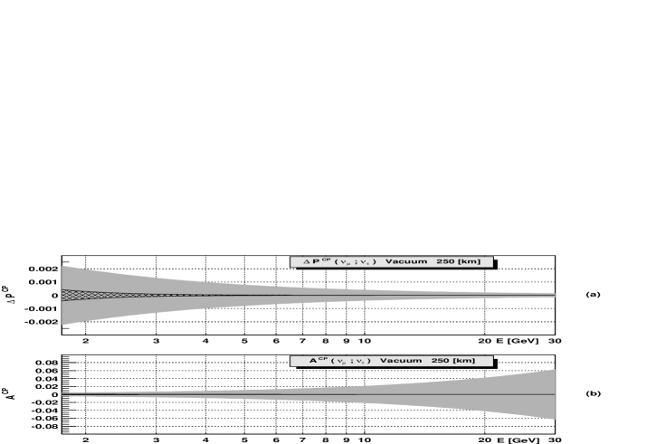
Figure 4: $\Delta P_{\mu\to\tau}^{CP}$ (a) and $A_{\mu\to\tau}^{CP}$ (b) for neutrino oscillations in vacuum, L=250 km. Other parameters as in Fig. 2a, $\epsilon_{\alpha}$ according to Eq. 82.

In Figs. 4a,4b the same quantities as in Figs. 3a,3b are presented but for the second set of $\epsilon_{\alpha}$ parameters (Eq. 82). As $\epsilon_{\mu}$ is 10 times smaller, also nonunitary effects are smaller by the same factor.

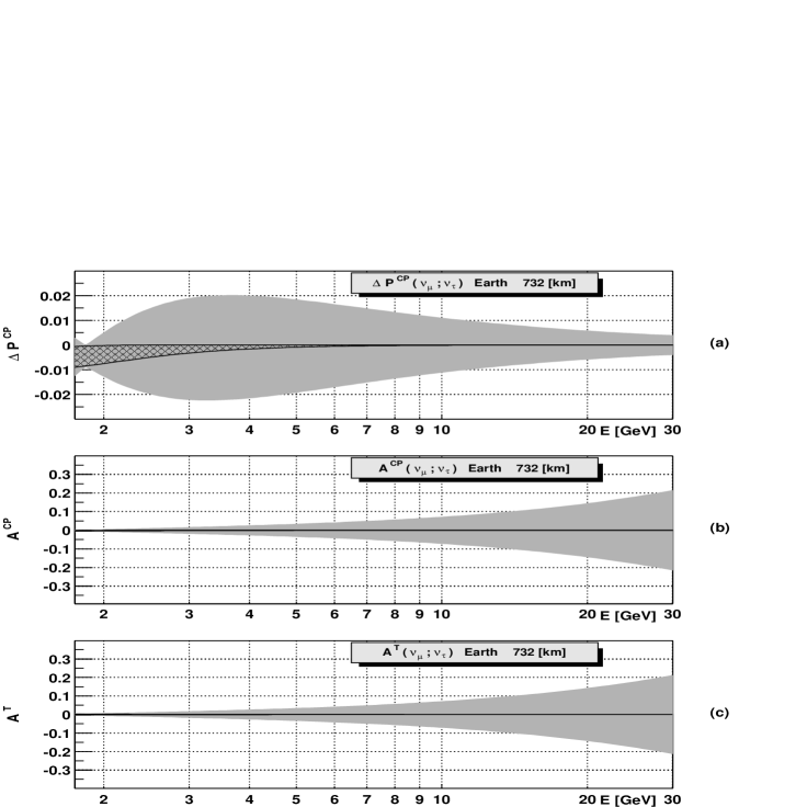
Figure 6: $\Delta P_{\mu\to\tau}^{CP}$ (a), $A_{\mu\to\tau}^{CP}$ (b), and $A_{\mu\to\tau}^{T}$ (c) for neutrino oscillations in matter, L=732 km. Other parameters as in Fig. 2a, $\epsilon_{\alpha}$ according to Eq. 81.

For L=250 km the effects of neutrino interactions in the Earth’s matter are small and all presented quantities are almost the same as in vacuum. Thus we do not present them here. However, for longer baseline experiments (L=732 km) matter effects can already be seen. In Figs. 5a,5b and Figs. 6a-c the $\Delta P_{\mu\to\tau}^{CP}$, $A_{\mu\to\tau}^{CP}$ and $A_{\mu\to\tau}^{T}$ quantities are presented for $\nu_{\mu}\to\nu_{\tau}$ transitions in vacuum and matter, respectively. The $\epsilon_{\alpha}$ parameters are taken according to Eq. 81. Again, the non-unitary effects are large. For the unitary case, the symmetric region of $\Delta P_{\mu\to\tau}^{CP}$ in vacuum (Fig. 5a) becomes asymmetric (negative) in matter (Fig. 6a). The full range of $\Delta P_{\mu\to\tau}^{CP}$ for non-unitary oscillations shifts also slightly toward negative values (compare the shaded regions in Fig. 5a and Fig. 6a). Once again $A_{\mu\to\tau}^{CP}$ (Fig. 5b and Fig. 6b) and $A_{\mu\to\tau}^{T}$ (Fig. 6c) asymmetries are very similar to each other. They are larger for higher neutrino energies but, unfortunately, not because $\Delta P_{\mu\to\tau}^{CP}$ is larger, but because the probabilities for (anti)neutrino oscillations are getting smaller.

V Conclusions

The evolution equation for neutrinos propagating in matter is found in the case when heavy neutrinos do not decouple and, as a result, the mixing matrix between light neutrinos is not unitary.

The neutrino propagation is described by a hermitian Hamiltonian found in the eigenmass basis of light neutrinos. This basis is the most convenient to calculate physical effects. Two other basis which we consider, that means the full orthogonal basis which contains both light and heavy neutrino states, and the ”experimental” basis with nonorthogonal light neutrinos only, are more complicated when applied to numerics. In the first case, the Hamiltonian is hermitian but has full $(3+n_{s}+n_{R})\times(3+n_{s}+n_{R})$ dimensions. In the second case, it has smaller $(3+n_{s})\times(3+n_{s})$ dimensions, but is represented by a non-hermitian matrix.

If heavy neutrinos do not decouple, the notion of neutrino flavour loose its meaning. In such case it is better to see active light neutrinos as particles produced together with charged leptons of particular flavours rather then particles having their own flavours. Moreover, the nonorthogonality of such neutrino states has also some impact on theoretically calculated cross sections for neutrino production and detection.

We have found the equation which describes the propagation of light neutrinos in any polarized, nonhomogeneous, charged matter. Numerical analysis is done in the simpler case of unpolarized, isotropic, and electrically neutral matter.

The non-unitary neutrino mixing is especially important for CP and T violating effects in neutrino oscillation. Two additional CP phases, which appear in the light-heavy neutrino mixing matrix, have crucial consequences in such phenomena.

In comparison with normal unitary neutrino oscillation, the CP and T violation are generally larger and appear even where standard effects are very small or vanish. The new CP and T violation effects depend on the strength of light-heavy neutrino mixing. For present experimental bounds on the non-decoupling parameters, the $\nu_{\mu}\to\nu_{\tau}$ oscillation is especially sensitive to the new CP effects. For $\nu_{e}\to\nu_{\mu}$ oscillation, where the bound on the $c_{e\mu}$ parameters coming from the non observation of the $\mu\to e\gamma$ decay are very stringent, the effects are smaller.

In the future, the observation of CP effects (or lack of them) in the $\nu_{\mu}\to\nu_{\tau}$ oscillation can give new information on the light-heavy neutrino mixing. The bounds on such mixing, found in future neutrino experiments, can be stronger then the same bounds coming from charged lepton violating processes.

VI Acknowledgments

The work was supported by the Polish Committee for Scientific Research under Grants 2P03B05418 and 2P03B13622.

Figure 1: Feynman diagrams for scattering of neutrinos in matter . All three diagrams contribute to neutrino-electron scattering $n_{i}+e^{-}\to n_{k}+e^{-}$ $(f=e)$. Only diagram (a) contributes to neutrino-nucleon scattering $n_{i}+f\to n_{k}+f$ $(f=p,n)$.

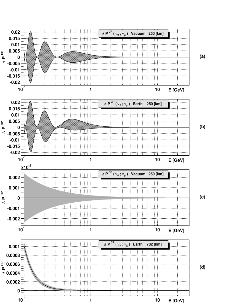
Figure 2:
(a) The probability difference $\Delta P_{e\to\mu}^{CP}$ defined in Eq. 67, for L=250 km as a function of neutrino energy (oscillations in vacuum). The hatched region describes normal unitary oscillations with $0<\delta\leq 2\pi$. The shaded region corresponds to the non-unitary neutrino oscillations with additional CP breaking phases $\chi_{1},\chi_{2}$ (Eq. 48) that change in the domain $0<\chi_{i}\leq 2\pi$. The $\epsilon_{\alpha}$ parameters for both sets from Eqs. 81,82 give $\epsilon_{e}\epsilon_{\mu}=10^{-4}$ and the results are the same for both cases. Other oscillation parameters correspond to the best LMA fit values given in best (see the text for details).
(b) Neutrino oscillations in matter with the same parameters as in Fig. 2a. In this case neutrinos pass only the first shell of the Earth’s interior irina with a constant density $\rho=2.6\;g/cm^{3}$ and $Y_{e}=0.494$.
(c) Neutrino oscillations in vacuum with the same parameters as in Fig. 2a but for $\Theta_{13}=0$. In this case, in vacuum $\Delta P_{\alpha\to\beta}^{CP}=0$ for normal unitary neutrino oscillations. Non-zero effects are exclusively related to the non-decoupling heavy neutrinos.
(d) $\Delta P_{e\to\mu}^{CP}$ for neutrino oscillations in matter for $\Theta_{13}=0$, L=732 km. Other parameters as in Fig. 2a. Because of matter effects, $\Delta P_{e\to\mu}^{CP}\neq 0$ even for unitary neutrino oscillations.

Figure 3: $\Delta P_{\mu\to\tau}^{CP}$ (a) and $A_{\mu\to\tau}^{CP}$ (b) for neutrino oscillations in vacuum, L=250 km. Other parameters as in Fig. 2a, $\epsilon_{\alpha}$ according to Eq. 81.

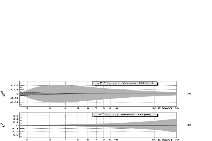
Figure 5: $\Delta P_{\mu\to\tau}^{CP}$ (a) and $A_{\mu\to\tau}^{CP}$ (b) for neutrino oscillations in vacuum, L=732 km. Other parameters as in Fig. 2a, $\epsilon_{\alpha}$ according to Eq. 81.