Radiative corrections to all charge assignments of heavy quark baryon semileptonic decays

Abstract

In semileptonic decays of spin-1/2 baryons containing heavy quarks up to six charge assignments for the baryons and lepton are possible. We show that the radiative corrections to four of these possibilities can be directly obtained from the final results of the two possibilities previously studied. There is no need to recalculate integrals over virtual or real photon momentum or any traces.

I Introduction

By necessity, the calculation of radiative corrections (RC) to spin-1/2 baryon semileptonic decays (BSD) requires that definite charges be chosen for the participating particles. In previous calculations [1] we have chosen a negatively charged emitted lepton and either a neutral or a negatively charged decaying baryon. This covers all of hyperon semileptonic decays, with the exception of $\Sigma^{+}\rightarrow\Lambda l^{+}\nu_{l}$. If the polarization of the baryons is not involved, the previous results can be extended [2] to cover this latter decay using a very practical rule, which also applies to $\Lambda_{c}^{+}\rightarrow\Lambda l^{+}\nu_{l}$. However, when heavy quarks are involved several other charge arrangements for the baryons appear, and then one faces the problem of having to recalculate the accompanying RC. In particular doubly-charged baryons must also be considered. Recently, preliminary evidence for double-charm baryons has been reported [3], so it is also timely to study the RC to semileptonic decays of such baryons. It is the purpose of this paper to obtain the RC to BSD with all the charge assignments to the baryons allowed when heavy quarks are involved. Our main result will show that with proper adaptations, the previous results obtained with the initial choices of baryon charges can also be used to obtain the RC to the other charge assignment possibilities.

Let us list the several types of BSD we have to discuss. For definiteness we shall take as a heavy quark the charm quark, i.e., we shall consider the four quarks $u$, $d$, $s$, and $c$. Their charges are $2/3$, $-1/3$, $-1/3$, and $2/3$ and their strong flavors are $S=0$, $0$, $-1$, $0$, $C=0$, $0$, $0$, $1$, and $I_{3}=1/2$, $-1/2$, $0$, $0$, respectively. Their semileptonic decays are

$$d \rightarrow ul^{-}\overline{\nu}_{l}\qquad\left(\Delta S=\Delta C=0,\;\Delta Q=1\right),$$ (1)

$$s \rightarrow ul^{-}\overline{\nu}_{l}\qquad\left(\Delta C=0,\;\Delta S=\Delta Q=1\right),$$ (2)

$$c \rightarrow sl^{+}\nu_{l}\qquad\left(\Delta S=\Delta C=\Delta Q=-1\right),$$ (3)

$$c \rightarrow dl^{+}\nu_{l}\qquad\left(\Delta S=0,\;\Delta C=\Delta Q=-1\right).$$ (4)

In parentheses we display the selection rules these decays obey, in terms of the charges and strong flavors involved. In addition, the Cabibbo-Kobayashi-Maskawa matrix elements should accompany these selection rules.

At the hadron level these quarks can form twenty baryons. Eight carry no charm, nine carry single charm, and three carry double charm. The semileptonic decays of these baryons are grouped into

$$A^{-}\rightarrow B^{0}(l^{-}\overline{\nu}_{l}),$$ (5)

$$A^{0}\rightarrow B^{+}(l^{-}\overline{\nu}_{l}),$$ (6)

$$A^{+}\rightarrow B^{0}(l^{+}\nu_{l}),$$ (7)

$$A^{0}\rightarrow B^{-}(l^{+}\nu_{l}),$$ (8)

$$A^{++}\rightarrow B^{+}(l^{+}\nu_{l}),$$ (9)

$$A^{+}\rightarrow B^{++}(l^{-}\overline{\nu}_{l}).$$ (10)

The BSD of the eight hyperons fall in the groups (5) or (6), with the exception of $\Sigma^{+}\rightarrow\Lambda l^{+}\nu_{l}$ which falls in group (7). Many charm baryon (or bottom baryon) decays will fall in some of the groups (5)-(7), but the last groups (8)-(10) necessarily require the intervention of charm. For completeness, let us list the BSD with appreciable phase-space according to the above groups. We use the naming scheme of Ref. [4], whose Greek symbol indicates isospin and subindex indicates heavy quark content. All of these decays are driven, at the quark level, by the semileptonic decays (2), (3), or (4),

$$\begin{array}[]{lll}{\rm Group\ (7)}:&\Omega_{cc}^{+}\rightarrow\Omega_{c}^{0}l^{+}\nu_{l},&\Omega_{cc}^{+}\rightarrow\Xi_{c}^{\prime\,0}\left(\Xi_{c}^{0}\right)l^{+}\nu_{l},\\ &\Xi_{cc}^{+}\rightarrow\Xi_{c}^{\prime\,0}\left(\Xi_{c}^{0}\right)l^{+}\nu_{l},&\Xi_{cc}^{+}\rightarrow\Sigma_{c}^{0}l^{+}\nu_{l},\\ &\Xi_{c}^{+}\rightarrow\Xi^{0}l^{+}\nu_{l},&\Xi_{c}^{+}\rightarrow\Lambda\left(\Sigma^{0}\right)l^{+}\nu_{l},\\ &\Lambda_{c}^{+}\rightarrow\Lambda\left(\Sigma^{0}\right)l^{+}\nu_{l},&\Lambda_{c}^{+}\rightarrow nl^{+}\nu_{l}.\\ {\rm Group\ (8)}:&\Xi_{c}^{0}\rightarrow\Xi^{-}l^{+}\nu_{l},&\Xi_{c}^{0}\rightarrow\Sigma^{-}l^{+}\nu_{l},\\ &\Omega_{c}^{0}\rightarrow\Sigma^{-}l^{+}\nu_{l}.\\ {\rm Group\ (9)}:&\Xi_{cc}^{++}\rightarrow\Xi^{\prime+}\left(\Xi_{c}^{+}\right)l^{+}\nu_{l},&\Xi_{cc}^{++}\rightarrow\Lambda_{c}^{+}\left(\Sigma_{c}^{+}\right)l^{+}\nu_{l}.\\ {\rm Group\ (10)}:&\Omega_{cc}^{+}\rightarrow\Sigma_{cc}^{++}l^{-}\overline{\nu}_{l},&\Xi_{c}^{+}\rightarrow\Sigma_{c}^{++}l^{-}\overline{\nu}_{l}.\end{array}$$ (19)

We have omitted above those decays with very small phase space driven by (1) and also those decays which are overwhelmed by strong decays, like $\Sigma_{c}\rightarrow\Lambda_{c}^{+}\pi,\;$or by electromagnetic decays, like $\Xi_{c}^{\prime\,0}\rightarrow\Xi_{c}^{0}\gamma$.

In what follows we shall obtain model-independent RC, according to the analyses of Refs. [5, 6], which include terms of zeroth and first order in $\left(\alpha/\pi\right)\left(q/M_{1}\right)^{0}$ and $\left(\alpha/\pi\right)\left(q/M_{1}\right),$ where $q$ is the four-momentum transfer and $M_{1}$ is the mass of $A.$ We shall not impose any kinematical constraint on the four-momentum of the bremsstrahlung photon, so that our results will be useful both in what in previous papers we referred to as the three-body and four-body regions. We shall allow for non-zero polarization $s_{1}$ of the decaying baryon $A$. Our first task is to extend the RC with polarized $A$ obtained for $l^{-}$ emission in groups (5) and (6), to decays with $l^{+}$ emission in groups (7) and (8). This is done in Sect. II. A simple and practical rule is obtained, analogous to the rule of Ref. [2]. The groups of decays involving double charge of one of the baryons will be discussed in Sect. III. Although this requires more effort, again a simple rule is obtained. Finally, in Sect. IV we discuss our analysis.

II RC to polarized baryon semileptonic decays with positively-charged lepton emission

When $A$ is not polarized the RC with $l^{+}$ emission in groups (7) and (8) are easily obtained from the final results of groups (5) and (6) when $l^{-}$ is emitted, using the rule of Ref. [2]. However, this rule does not apply to the RC to the part of the differential decay rate, and along with it to the Dalitz plot (DP) containing the polarization of $A$. It is the purpose of this section to obtain the corresponding rule. To do this requires that we review the calculation of RC at intermediate steps and trace the changes introduced by $l^{+}$ emission. The rule will allow us to use the final expressions with $l^{-}$ emission to obtain directly the final result with $l^{+}$ emission.

A Virtual RC

We shall first discuss the decays $A^{0}\rightarrow B^{-}l^{+}\nu_{l}$ of group (8). The calculation of its virtual RC follows the same steps of the corresponding calculation of $A^{0}\rightarrow B^{+}l^{-}\overline{\nu}_{l}$ of group (6). These corrections are split into a finite, calculable, and model-independent part and into a model-dependent one, which can be absorbed into the form factors of the uncorrected amplitude ${\sf M}_{0}$. This last is indicated by putting primes on the form factors and ${\sf M}_{0}$. Thus, the decay amplitude with virtual radiative corrections turns out to be ${\sf M}_{V}={\sf M}_{0}^{\prime}+{\sf M}_{v}^{i}$, where ${\sf M}_{0}^{\prime}=(G_{V}/\sqrt{2})H_{\lambda}^{\prime}L_{\lambda}^{\mp}$, with $H_{\lambda}^{\prime}={\overline{u}}_{2}\left(p_{2}\right)W_{\lambda}^{\prime}u_{1}\left(p_{1}\right)$, $L_{\lambda}^{-}=\overline{u}_{l}O_{\lambda}v_{\nu}$, $L_{\lambda}^{+}=\overline{u}_{\nu}O_{\lambda}v_{l}$, whereas ${\sf M}_{v}^{i}$, after integrations over the virtual photon four-momentum, is given by

$${\sf M}_{v}^{i}=\frac{\alpha}{\pi}\frac{G_{V}}{\sqrt{2}}H_{\lambda}\left[L_{\lambda}^{\mp}\phi\pm\left\{\begin{array}[]{l}{\overline{u}}_{l}{\not\!p}_{2}O_{\lambda}v_{\nu}\\ \overline{u}_{\nu}O_{\lambda}{\not\!p}_{2}v_{l}\end{array}\right\}\phi^{\prime}\right],$$ (22)

On the other hand, $W_{\lambda}^{\prime}$ is defined as

$$W_{\lambda}^{\prime}=\gamma_{\lambda}\left(f_{1}^{\prime}+g_{1}^{\prime}\gamma_{5}\right)+\sigma_{\lambda\alpha}\left(q_{\alpha}/M_{1}\right)\left(f_{2}^{\prime}+g_{2}^{\prime}\gamma_{5}\right)+\left(q_{\lambda}/M_{1}\right)\left(f_{3}^{\prime}+g_{3}^{\prime}\gamma_{5}\right),$$ (23)

with $O_{\lambda}=\gamma_{\lambda}\left(1+\gamma_{5}\right)$. Our metric and $\gamma$-matrix convention are those of Ref. [1]. In (11) the upper (lower) sign refers to the upper (lower) sign of $A^{0}\rightarrow B^{\pm}l^{\mp}\nu_{l}$. The spinors $u_{1}$ and $u_{2}$ belong to $A$ and $B$, respectively.

Our interest here is in polarized decaying baryons $A$ along $s_{1}$, so we shall concentrate on this part of the transition probability. In ${\sf M}_{V}$ one must replace $u_{1}\to\Sigma({\not\!s}_{1})u_{1}$, with $\Sigma({\not\!s}_{1})=(1-\gamma_{5}{\not\!s}_{1})/2$, square ${\sf M}_{V}$ and sum over spins. Extracting the part that contains $s_{1}$, we obtain

$$\sum_{s}\left|{\sf M}_{V}^{(s)}\right|^{2} = \frac{1}{2}\sum_{s}\left|{\sf M}_{0}^{\prime\;(s)}\right|^{2}+\frac{1}{2}c_{2}{\rm Tr}\left[\left({\not\!p}_{2}+M_{2}\right)W_{\lambda}\gamma_{5}{\not\!s}_{1}\left({\not\!p}_{1}+M_{1}\right){\overline{W}}_{\mu}\right]$$ (25)

$$\times\left\{\left({\rm Re}\ \phi\right){\rm Tr}\left[{\not\!\,l}\gamma_{\lambda}{\not\!p}_{\nu}\gamma_{\mu}\left(1\pm\gamma_{5}\right)\right]+\left({\rm Re}\ \phi^{\prime}\right){\rm Tr}\left[{\not\!p}_{2}\gamma_{\lambda}{\not\!p}_{\nu}\gamma_{\mu}\left(1\pm\gamma_{5}\right)\right]\right\}.$$

The explicit forms of $\phi$, $\phi^{\prime}$, and the constant $c_{2}$ are not relevant here. They can be found in Ref. [7]. All we need to know is that $c_{2}$ is real and only the real part of $\phi$ and $\phi^{\prime}$ appear in (13). $l$ and $p_{\nu}$ are the four-momenta of $l^{\mp}$ and the accompanying neutrino, respectively.

Equation (13) is a real quadratic function of the form factors $f_{i}^{\prime}$ and $g_{i}^{\prime}$. If we assume momentarily $g_{i}^{\prime}=0$ we obtain a hadronic trace containing only one $\gamma_{5}$. If instead we assume $f_{i}^{\prime}=0$, we obtain $(\gamma_{5})^{3}=\gamma_{5}$ in this trace. Thus, the hadronic part of (13) containing non-interference $f_{i}^{\prime}f_{j}^{\prime}$ and $g_{i}^{\prime}g_{j}^{\prime}$ products is imaginary. The interference products $f_{i}^{\prime}g_{j}^{\prime}$ give $(\gamma_{5})^{2}=1$ in this trace. Accordingly, the part of the trace containing these products is real.

The leptonic trace also contains a real part and an imaginary one, this latter coming from the $\gamma_{5}$ contribution. Since Eq. (13) is necessarily real and the double sign is attached to the $\gamma_{5}$ in the leptonic trace, we can now obtain the rule we are looking for: to use the results of the polarization part of $l^{-}$ emission of decays (6) for $l^{+}$ emission of decays (8), one must reverse the signs of all the non-interference products of form factors and keep the same signs in the interference products. This rule should be contrasted with the rule in the unpolarized decay rate [2]; it is the opposite, so to speak. We did not discuss the changes in the ${\sf M}_{0}^{\prime\,(s)}$ contribution to Eq. (13). One can readily see that one obtains the same rule. Also, the rule to connect decays (7) with decays (5) is immediate.

B Bremsstrahlung RC

Again we shall discuss first the group of decays $A^{0}\rightarrow B^{\pm}l^{\mp}\nu_{l}\gamma$, where $\gamma$ is a real photon of four-momentum $k$. The transition amplitude contains three terms,

$${\sf M}_{B}={\sf M}_{B_{1}}+{\sf M}_{B_{2}}+{\sf M}_{B_{3}}.$$ (26)

The Low theorem [6], in the form presented by Chew [8], allows us to get

$${\sf M}_{B_{1}} = \pm\frac{eG_{V}}{\sqrt{2}}\epsilon_{\mu}\left(\frac{l_{\mu}}{l\cdot k}-\frac{p_{2\mu}}{p_{2}\cdot k}\right)H_{\lambda}L_{\lambda}^{\mp},$$ (27)

$${\sf M}_{B_{2}} = \pm\frac{eG_{V}}{\sqrt{2}}\epsilon_{\mu}H_{\lambda}\frac{1}{2l\cdot k}\left\{\begin{array}[]{l}\overline{u}_{l}\gamma_{\mu}{\not\!k}O_{\lambda}v_{\nu}\\ \overline{u}_{\nu}O_{\lambda}{\not\!k}\gamma_{\mu}v_{l}\end{array}\right\},$$ (30)

$${\sf M}_{B_{3}} = \pm\frac{eG_{V}}{\sqrt{2}}\epsilon_{\mu}{\overline{u}}_{2}T_{\mu\lambda}u_{1}L_{\lambda}^{\mp}.$$ (31)

Here $e$ (a negative number) is the charge of $l^{-}$ and $\epsilon_{\mu}$ is the polarization four-vector of $\gamma$. $H_{\lambda}$, $L_{\lambda}^{\mp}$, and the upper and lower signs have the same meaning as before. The tensor $T_{\mu\lambda}$ is given by

$$T_{\mu\lambda} = \frac{1}{2p_{2}\cdot k}\left[-\gamma_{\mu}{\not\!k}-\frac{\kappa_{2}}{e_{2}}\sigma_{\mu\alpha}k_{\alpha}\left({\not\!p}_{2}+{\sf M}_{2}\right)\right]W_{\lambda}$$ (34)

$$\mbox{}+\frac{1}{2p_{1}\cdot k}W_{\lambda}\frac{\kappa_{1}}{e_{2}}\left({\not\!p}_{1}+M_{1}\right)\sigma_{\mu\alpha}k_{\alpha}$$

$$\mbox{}+\left(\frac{p_{2\mu}k_{\rho}}{p_{2}\cdot k}-g_{\mu\rho}\right)\left(\sigma_{\lambda\rho}\frac{f_{2}+g_{2}\gamma_{5}}{M_{1}}+g_{\lambda\rho}\frac{f_{3}+g_{3}\gamma_{5}}{M_{1}}\right),$$

where $\kappa_{1}$ and $\kappa_{2}$ are the anomalous magnetic moments of $A^{0}$ and $B^{\pm}$, respectively, and $e_{2}$ is the charge of $B^{\pm}$. Again we shall concentrate on the part of the bremsstrahlung transition rate that contains the polarization $s_{1}$ of $A^{0}$. Introducing $\Sigma({\not\!s}_{1})u_{1}$ in ${\sf M}_{B}$, squaring ${\sf M}_{B}$, and summing over spins, one can extract the polarization part of the transition probability. The result is

$$\sum_{s,\epsilon}\left|{\sf M}_{B}^{(s)}\right|^{2} = c_{3}{\rm Re}\sum_{\epsilon}\epsilon_{\alpha}\epsilon_{\beta}\left\{{\rm Tr}\left[\left({\not\!p}_{2}+M_{2}\right)W_{\lambda}\gamma_{5}{\not\!s}_{1}\left({\not\!p}_{1}+M_{1}\right)\overline{W}_{\mu}\right]\right.$$ (40)

$$\mbox{}\times\left[I^{\alpha}I^{\beta}{\rm Tr}\left[{\not\!\,l}\gamma_{\lambda}{\not\!p}_{\nu}\gamma_{\mu}\left(1\pm\gamma_{5}\right)\right]\right.$$

$$\mbox{}+\left(\frac{1}{2l\cdot k}\right)^{2}{\rm Tr}\left[{\not\!k}\gamma_{\beta}{\not\!\,l}\gamma_{\alpha}{\not\!k}\gamma_{\lambda}{\not\!p}_{\nu}\gamma_{\mu}\left(1\pm\gamma_{5}\right)\right]$$

$$\mbox{}+\left.\frac{I^{\alpha}}{l\cdot k}{\rm Tr}\left[{\not\!k}\gamma_{\beta}{\not\!\,l}\gamma_{\lambda}{\not\!p}_{\nu}\gamma_{\mu}(1\pm\gamma_{5})\right]\right]$$

$$\mbox{}+{\rm Tr}\left[({\not\!p}_{2}+M_{2})T_{\alpha\lambda}\gamma_{5}{\not\!s}_{1}\left({\not\!p}_{1}+M_{1}\right)\overline{W}_{\mu}\right]$$

$$\mbox{}\left.\times\left[2I_{\beta}{\rm Tr}\left[{\not\!\,l}\gamma_{\lambda}{\not\!p}_{\nu}\gamma_{\mu}\left(1\pm\gamma_{5}\right)\right]+\frac{1}{l\cdot k}{\rm Tr}\left[{\not\!k}\gamma_{\beta}{\not\!\,l}\gamma_{\lambda}{\not\!p}_{\nu}\gamma_{\mu}\left(1\pm\gamma_{5}\right)\right]\right]\right\}.$$

Here $c_{3}$ is an overall real constant containing $\alpha$, $G_{V}$, etc., and $I_{\alpha}=(l_{\alpha}/l\cdot k)-p_{2_{\alpha}}/p_{2}\cdot k)$. The first three terms in Eq. (18) come from the squares and interference of ${\sf M}_{B_{1}}$ and ${\sf M}_{B_{2}}$. The hadronic trace in them is the same one as in Eq. (13). Therefore, the non-interference products $f_{i}^{\prime}f_{j}^{\prime}$ and $g_{i}^{\prime}g_{j}^{\prime}$ are accompanied by a $\gamma_{5}$ and the interference products $f_{i}^{\prime}g_{j}^{\prime}$ are not. The reality condition on Eq. (18) and the double sign in front of the $\gamma_{5}$ in the leptonic trace lead to the same rule of the virtual RC.

The last two terms of Eq. (18) contain T_αλ in the hadronic trace. Using Eq. (17) they can be rearranged into the sum of

$${\rm Tr}\left[({\not\!p}_{2}+M_{2})\gamma_{\alpha}{\not\!k}W_{\lambda}\gamma_{5}{\not\!s}_{1}({\not\!p}_{1}+M_{1})\overline{W}_{\mu}\right],$$ (41)

$${\rm Tr}\left[({\not\!p}_{2}+M_{2})\sigma_{\alpha\beta}k_{\rho}({\not\!p}_{2}+M_{2})W_{\lambda}\gamma_{5}{\not\!s}_{1}({\not\!p}_{1}+M_{1})\overline{W}_{\mu}\right],$$ (42)

$${\rm Tr}\left[({\not\!p}_{2}+M_{2}))\sigma_{\lambda\alpha}(f_{2}+g_{2}\gamma_{5})\gamma_{5}{\not\!s}_{1}({\not\!p}_{1}+M_{1})\overline{W}_{\mu}\right],$$ (43)

and

$${\rm Tr}\left[({\not\!p}_{2}+M_{2})g_{\lambda\alpha}(f_{3}+g_{3}\gamma_{5})\gamma_{5}{\not\!s}_{1}({\not\!p}_{1}+M_{1})\overline{W}_{\mu}\right].$$ (44)

Let us now follow the same steps as before. Assuming momentarily all $g_{i}=0$ or all $f_{i}=0$ we see that these traces contain either $\gamma_{5}$ or $(\gamma_{5})^{3}$. So the traces with non-interference products are imaginary numbers. The traces with interference products do not contain $\gamma_{5}$ and are accordingly real numbers. Then, the reality condition on Eq. (18) and the position of the double sign in front of the $\gamma_{5}$ in the leptonic trace lead to the same rule as before.

Collecting all the previous results we can establish the complete rule to obtain the RC to the polarization part of decay $A^{0}\rightarrow B^{-}l^{+}\nu_{l}$ directly from the final RC to the polarization part of $A^{0}\rightarrow B^{+}l^{-}\overline{\nu}_{l}$: one must reverse the signs of the non-interference products $f_{i}^{\prime}f_{j}^{\prime}$ and $g_{i}^{\prime}g_{j}^{\prime}$ and keep the same sign of the interference products $f_{i}^{\prime}g_{j}^{\prime}$. It is clear that this rule covers contributions of orders $\left(\alpha/\pi\right)\left(q/M_{1}\right)^{0}$ and $\left(\alpha/\pi\right)\left(q/M_{1}\right)$.

The same analysis applies to the decays $A^{\pm}\rightarrow B^{0}l^{\pm}\nu_{l}$ of groups (5) and (7) and one comes to the same rule: the RC to the polarization part of $A^{+}\rightarrow B^{0}l^{+}\nu_{l}$ are obtained from the final result of the RC to the polarization part of $A^{-}\rightarrow B^{0}l^{-}\overline{\nu}_{l}$ by reversing the signs in front of the products $f_{i}^{\prime}f_{j}^{\prime}$ and $g_{i}^{\prime}g_{j}^{\prime}$ and keeping the same sign in front of the products $f_{i}^{\prime}g_{j}^{\prime}$.

As already mentioned, this rule is, so to speak, the opposite to the rule that applies in the unpolarized decay rate. In this case the interference products of form factors must reverse their signs, while the non-interference ones preserve their signs. Equivalently, one can cover both polarized and unpolarized cases by restating the rules as to change the signs of all $g_{i}$ form factors and the sign of $s_{1}$. In the literature there exists another rule [9] to change the results with $l^{-}$ emission into the final results with $l^{+}$ emission. This rule is given in terms of the lepton four-momenta. One clearly sees that it is not of practical use when RC are incorporated.

To close this section, let us remark that the rule obtained is applicable to any $l^{+}$ $(e^{+},\mu^{+},\tau^{+})$. It applies in any Lorentz frame, and it is valid in both the three-body and four-body regions of the DP.

III RC to semileptonic decays with double-charge baryons

To study the RC to decays in groups (9) and (10) requires that we start at the graph level, extending the work of Refs. [5, 6]. For definiteness, we shall discuss decays of type (9) and at the end we shall include the decays of type (10).

A Virtual RC

The Feynman diagrams for decays (9) are displayed in Fig. 1. The blobs stand for the effects of strong interactions and details of weak interactions. Our notation and conventions are those of Ref. [5].

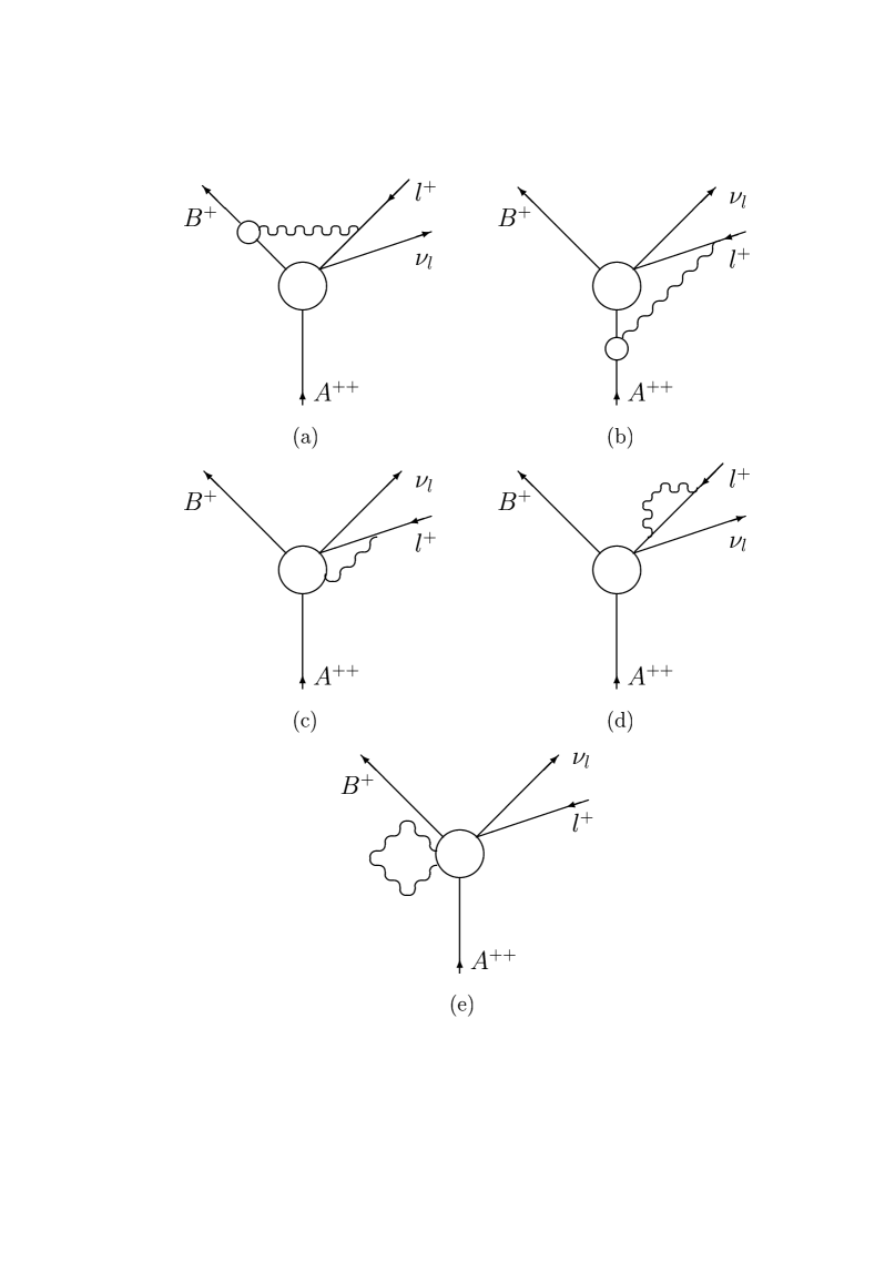
FIG. 1.: Feynman graphs for virtual RC to BSD. The blobs stand for strong interaction effects and details of weak interactions.

The virtual RC can be split into a finite and model-independent part and into a model-dependent one. In diagrams 1(a), 1(b), and 1(c) the virtual photon is interchanged between $l^{+}$ and a charge line within $B^{+}$, within $A^{++}$, and within the weak vertex, respectively. The three diagrams lead to a transition amplitude that can be cast into the form

$${\sf M}_{v_{1}} = -\frac{G_{V}}{\sqrt{2}}\frac{\alpha}{4\pi^{3}}\frac{1}{i}\int d^{4}kD_{\mu\alpha}(k)\left\{\overline{u}_{2}\left[2W_{\lambda}(p_{2},p_{1})\frac{(2p_{1\mu}-k_{\mu})}{k^{2}-2p_{1}\cdot k+i\varepsilon}+T_{\mu\lambda}^{+}(p_{1},p_{2},k)\right.\right.$$ (46)

$$\mbox{}+\left.\left.\left(\frac{2p_{2\mu}+k_{\mu}}{k^{2}+2p_{2}\cdot k+i\varepsilon}W_{\lambda}(p_{2},p_{1})+T_{\mu\lambda}^{0}(p_{1},p_{2},k)\right)\right]u_{1}\right\}\overline{u}_{\nu}O_{\lambda}\frac{2l_{\alpha}-{\not\!k}\gamma_{\alpha}}{k^{2}-2l\cdot k+i\varepsilon}v_{l}.$$

Here $l$, $k$, $p_{2}$, and $p_{1}$ are the four-momenta of $l^{+}$, the virtual photon, $B^{+}$, and $A^{++}$, respectively. All the model dependence in these diagrams is contained in the tensors $T_{\mu\nu}^{+}$ and $T_{\mu\nu}^{0}$. Their upper indices will be explained shortly. The other terms are model-independent.

Diagram 1(d), after wavefunction renormalization, leads to the amplitude

$${\sf M}_{v_{2}}=\frac{\alpha}{8\pi^{3}i}\frac{G_{V}}{\sqrt{2}}\overline{u}_{2}W_{\lambda}(p_{1},p_{2})u_{1}\int d^{4}kD_{\mu\alpha}(k)\overline{u}_{\nu}O_{\lambda}\left({\not\!\,l}-m\right)\frac{(2l_{\mu}+\gamma_{\mu}{\not\!k}){\not\!\,l}(2l_{\alpha}+{\not\!k}\gamma_{\alpha})}{2m^{2}\left(k^{2}+2l\cdot k+i\varepsilon\right)^{2}}v_{l}.$$ (47)

Notice that here the RC is contained only within the lepton covariant.

The last diagram 1(e) contains [10] a convection-convection contribution ${\sf M}_{v_{3}}^{c}$ which is model-independent and implements gauge invariance when it is added to Eqs. (20) and (21). The complete amplitude of Fig. 1(e) is then

$${\sf M}_{v_{3}}={\sf M}_{v_{3}}^{c}+{\sf M}_{v_{3}}^{\prime},$$ (48)

where

$${\sf M}_{v_{3}}^{c} = \frac{G_{V}}{\sqrt{2}}\frac{\alpha}{8\pi^{3}i}\overline{u}_{2}W_{\lambda}(p_{2},p_{1})u_{1}\overline{u}_{\nu}O_{\lambda}v_{l}\int d^{4}kD_{\mu\alpha}(k)$$ (50)

$$\mbox{}\times\left\{-\frac{(2p_{2}-k)_{\mu}\left(2p_{2}-k\right)_{\alpha}}{\left(k^{2}-2p_{2}\cdot k+i\varepsilon\right)^{2}}+2\frac{\left(2p_{1}-k\right)_{\mu}\left(2p_{1}-k\right)_{\alpha}}{\left(k^{2}-2p_{1}\cdot k+i\varepsilon\right)^{2}}\right\}.$$

All the model dependence of this diagram is contained in ${\sf M}_{v3}^{\prime}$.

The analysis of Ref. [5] to deal with the model-dependent parts contained in Eqs. (20) and (22), limited to small $q$, can be extended as shown in Ref. [11] to include contributions of order $(\alpha/\pi)(q/M_{1})$. The result of this extension is that up to this order all the model dependence has the same form as the uncorrected ${\sf M}_{0}$ and this allows that it be completely absorbed into the six already existing form factors. We indicate this by putting a prime on each form factors and on ${\sf M}_{0}$, too.

Let us deal with the model-independent parts in Eqs. (20), (21), and (23). The way Eq. (20) is written makes it easy to see that it can be rearranged into

$${\sf M}_{v_{1}}(A^{++}\rightarrow B^{+}l^{+}\nu_{l})=2{\sf M}_{v_{1}}(A^{+}\rightarrow B^{0}l^{+}\nu_{l})-{\sf M}_{v_{1}}(A^{0}\rightarrow B^{-}l^{+}\nu_{l}).$$ (51)

This amplitude has been rewritten as a linear combination of the amplitudes of the two BSD indicated in parentheses on the rhs. This explains the choice of upper indices on the $T_{\mu\nu}$ of Eq. (20). Notice the factor two and the minus sign in this rhs. The Coulomb contribution, attractive in $A^{0}\rightarrow B^{-}l^{+}\nu_{l}$, becomes repulsive in $A^{++}\rightarrow B^{+}l^{+}\nu_{l}$, as expected.

Equation (21) can be rearranged analogously. The amplitude ${\sf M}_{v_{2}}$ here is the same as ${\sf M}_{v_{2}}$ of $A^{+}\rightarrow B^{0}l^{+}\nu_{l}$ and of $A^{0}\rightarrow B^{-}l^{+}\nu_{l}$. So, one immediately gets

$${\sf M}_{v_{2}}(A^{++}\rightarrow B^{+}l^{+}\nu_{l})=2{\sf M}_{v_{2}}(A^{+}\rightarrow B^{0}l^{+}\nu_{l})-{\sf M}_{v_{2}}(A^{0}\rightarrow B^{-}l^{+}\nu_{l}).$$ (52)

Equation (23) can also be cast into the same linear combination, namely,

$${\sf M}_{v_{3}}(A^{++}\rightarrow B^{+}l^{+}\nu_{l})=2{\sf M}_{v_{3}}(A^{+}\rightarrow B^{0}l^{+}\nu_{l})-{\sf M}_{v_{3}}(A^{0}\rightarrow B^{-}l^{+}\nu_{l}).$$ (53)

The transition amplitude with virtual RC becomes,

$${\sf M}_{V}(A^{++}\rightarrow B^{+}l^{+}\nu_{l})=2\left[{\sf M}_{0}^{\prime}+{\sf M}_{v}(A^{+}\rightarrow B^{0}l^{+}\nu_{l})\right]-\left[{\sf M}_{0}^{\prime}+{\sf M}_{v}(A^{0}\rightarrow B^{-}l^{+}\nu_{l})\right],$$ (54)

where we added and subtracted ${\sf M}_{0}^{\prime}$, and ${\sf M}_{v}$ stand for the sum of the three virtual model-independent RC. The square brackets contain the transition amplitudes with virtual RC of $A^{+}\rightarrow B^{0}l^{+}\nu_{l}$ and $A^{0}\rightarrow B^{-}l^{+}\nu_{l}$. Equation (27) can be compactly rewritten as

$${\sf M}_{V}(A^{++}\rightarrow B^{+}l^{+}\nu_{l})=2{\sf M}_{V}(A^{+}\rightarrow B^{0}l^{+}\nu_{l})-{\sf M}_{V}(A^{0}\rightarrow B^{-}l^{+}\nu_{l}).$$ (55)

This analysis can be repeated step by step for $A^{+}\rightarrow B^{++}l^{-}\overline{\nu}_{l}$. The result is

$${\sf M}_{V}(A^{+}\rightarrow B^{++}l^{-}\overline{\nu}_{l})=2{\sf M}_{V}(A^{0}\rightarrow B^{+}l^{-}\overline{\nu}_{l})-{\sf M}_{V}(A^{-}\rightarrow B^{0}l^{-}\overline{\nu}_{l}).$$ (56)

Now the Coulomb interaction is attractive and the double charge of $B^{++}$ is taken care of by the factor two in front of the first term on the rhs of Eq. (29).

All the integrals over the virtual photon four-momentum required to get the virtual RC to $A^{++}\rightarrow B^{+}l^{+}\nu_{l}$ and $A^{+}\rightarrow B^{++}l^{-}\overline{\nu}_{l}$ can be taken from previous work [2, 7, 12]. ${\sf M}_{V}(A^{+}\rightarrow B^{0}l^{+}\nu_{l})$ and ${\sf M}_{V}(A^{0}\rightarrow B^{-}l^{+}\nu_{l})$ are given in Ref. [2]. ${\sf M}_{V}(A^{0}\rightarrow B^{+}l^{-}\overline{\nu}_{l})$ and ${\sf M}_{V}(A^{-}\rightarrow B^{0}l^{-}\overline{\nu}_{l})$ are given in Refs. [7, 12].

To obtain the differential decay rates and the DP corresponding to amplitudes (28) and (29), one follows the usual steps of squaring, summing and averaging over spins, and so on. For polarized decaying baryons one must replace $u_{1}$ by $\Sigma({\not\!s}_{1})u_{1}$. However, one must remember that the masses and form factors to be used in the rhs of Eqs. (28) and (29) are those of their lhs. We shall now show that at the differential decay rate level one obtains to first order in $\alpha/\pi$ the same linear combinations as at the amplitude level. Let us discuss again $A^{++}\rightarrow B^{+}l^{+}\nu_{l}$.

From Ref. [2] one has that

$${\sf M}_{V}(A^{0}\rightarrow B^{-}l^{+}\nu_{l})={\sf M}_{0}^{\prime}+\frac{\alpha}{\pi}({\sf M}_{0}\phi+{\sf M}_{p_{2}}\phi^{\prime})$$ (57)

and

$${\sf M}_{V}(A^{+}\rightarrow B^{0}l^{+}\nu_{l})={\sf M}_{0}^{\prime}+\frac{\alpha}{2\pi}({\sf M}_{0}\Phi+{\sf M}_{p_{1}}\Phi^{\prime}).$$ (58)

Equation (28) leads to

$$\sum\left|{\sf M}_{V}(A^{++}\rightarrow B^{+}l^{+}\nu_{l})\right|^{2} = 4\sum\left|{\sf M}_{V}(A^{+}\rightarrow B^{0}l^{+}\nu_{l})\right|^{2}+\sum\left|{\sf M}_{V}(A^{0}\rightarrow B^{-}l^{+}\nu_{l})\right|^{2}$$ (60)

$$\mbox{}-4{\rm Re}\sum{\sf M}_{V}(A^{+}\rightarrow B^{0}l^{+}\nu_{l})\overline{{\sf M}}_{V}(A^{0}\rightarrow B^{-}l^{+}\nu_{l}).$$

The bar means transpose conjugate. The cross term becomes, after substituting (30) and (31) and keeping only first order terms in $(\alpha/\pi)$,

$$-4{\rm Re}\sum{\sf M}_{V}\left(A^{+}\rightarrow B^{0}l^{+}\nu_{l}\right)\overline{{\sf M}}_{V}\left(A^{0}\rightarrow B^{-}l^{+}\nu_{l}\right)$$ (61)

$$=-2\left\{\left[\sum\left|{\sf M}_{0}^{\prime}\right|^{2}+\frac{\alpha}{2\pi}2{\rm Re}\sum{\sf M}_{0}^{\prime}\overline{({\sf M}_{0}\Phi+{\sf M}_{p_{1}}\Phi^{\prime})}\right]\right.$$ (62)

$$\mbox{\hglue 28.45274pt}+\left.\left[\sum\left|{\sf M}_{0}^{\prime}\right|^{2}+\frac{\alpha}{\pi}2{\rm Re}\sum({\sf M}_{0}\phi+{\sf M}_{p_{2}}\phi^{\prime})\overline{{\sf M}_{0}^{\prime}}\right]\right\}.$$ (63)

One can recognize within the brackets on the rhs the squares of the amplitudes (30) and (31) to first order in $(\alpha/\pi)$. Thus Eq. (33) becomes

$$-4{\rm Re}\sum{\sf M}_{V}\left(A^{+}\rightarrow B^{0}l^{+}\nu_{l}\right)\overline{{\sf M}}_{V}(A^{0}\rightarrow B^{-}l^{+}\nu_{l})$$ (64)

$$\mbox{\hglue 28.45274pt}=-2\sum\left|{\sf M}_{V}(A^{+}\rightarrow B^{0}l^{+}\nu_{l})\right|^{2}-2\sum\left|{\sf M}_{V}(A^{0}\rightarrow B^{-}l^{+}\nu_{l})\right|^{2}.$$ (65)

Collecting results the differential decay rate for $A^{++}\rightarrow B^{+}l^{+}\nu_{l}$ becomes

$$d\Gamma_{V}(A^{++}\rightarrow B^{+}l^{+}\nu_{l})=2d\Gamma_{V}(A^{+}\rightarrow B^{0}l^{+}\nu_{l})-d\Gamma_{V}(A^{0}\rightarrow B^{-}l^{+}\nu_{l}).$$ (66)

Exactly the same steps and using again Ref. [2] lead to

$$d\Gamma_{V}(A^{+}\rightarrow B^{++}l^{-}\overline{\nu}_{l})=2d\Gamma_{V}(A^{0}\rightarrow B^{+}l^{-}\overline{\nu}_{l})-d\Gamma_{V}(A^{-}\rightarrow B^{0}l^{-}\overline{\nu}_{l}).$$ (67)

Equations (35) and (36) show that we can use directly the decay rates previously obtained to get the decay rates of groups (9) and (10), without having to repeat the calculation of neither the virtual photon integrals nor the traces. Of course the form factors and masses appropriate to these decays must be used in the previous results.

B Bremsstrahlung RC

FIG. 2.: Feynman graphs for BSD with real photon emission. The blobs stand for strong interaction effects and details of weak interactions.

The Feynman diagrams with real photon emission of decays of group (9) are displayed in Fig. 2. The blob stands for strong-interaction effects and details of weak interactions. The Low theorem [6] allows the inclusion of terms of up to order $(\alpha/\pi)(q/M_{1})$ in a model-independent fashion. We shall use the approach of Chew [8] to use this theorem. The transition amplitude of the diagrams in Fig. 2 can be split into three contributions,

$${\sf M}_{B}(A^{++}\rightarrow B^{+}l^{+}\nu_{l}\gamma)={\sf M}_{B_{1}}+{\sf M}_{B_{2}}+{\sf M}_{B_{3}},$$ (68)

with

$${\sf M}_{B_{1}} = -e{\sf M}_{0}\left[\frac{\epsilon\cdot l}{l\cdot k}-2\frac{\epsilon\cdot p_{1}}{p_{1}\cdot k}+\frac{\epsilon\cdot p_{2}}{p_{2}\cdot k}\right],$$ (69)

$${\sf M}_{B_{2}} = -e\frac{G_{V}}{\sqrt{2}}\epsilon_{\mu}\,\overline{u}_{2}W_{\lambda}u_{1}\,\overline{u}_{\nu}O_{\lambda}\frac{\not{k}\gamma_{\mu}}{2l\cdot k}v_{l},$$ (70)

and

$${\sf M}_{B_{3}} = \frac{G_{V}}{\sqrt{2}}\overline{u}_{\nu}O_{\lambda}\,v_{l}\,\epsilon_{\mu}\,\overline{u}_{2}\,\left\{-2eW_{\lambda}\frac{{\not\!k}\gamma_{\mu}}{2p_{1}\cdot k}-\kappa_{1}W_{\lambda}\frac{{\not\!p}_{1}+M_{1}}{2p_{1}\cdot k}\sigma_{\mu\nu}k_{\nu}\right.$$ (74)

$$\mbox{}-e\frac{\gamma_{\mu}{\not\!k}}{2p_{2}\cdot k}W_{\lambda}+\kappa_{2}\sigma_{\mu\nu}k_{\nu}\frac{{\not\!p}_{2}+M_{2}}{2p_{2}\cdot k}W_{\lambda}$$

$$\mbox{}-2e\left[\frac{p_{1\mu}\,}{p_{1}\cdot k}k_{\rho}-g_{\mu\rho}\right]\left[\sigma_{\rho\lambda}\frac{f_{2}+g_{2}\gamma_{5}}{M_{1}}+g_{\rho\lambda}\frac{f_{3}+g_{3}\gamma_{5}}{M_{1}}\right]$$

$$\mbox{}+\left.e\left[\frac{p_{2\mu}\,}{p_{2}\cdot k}k_{\rho}-g_{\mu\rho}\right]\left[\sigma_{\rho\lambda}\frac{f_{2}+g_{2}\gamma_{5}}{M_{1}}+g_{\rho\lambda}\frac{f_{3}+g_{3}\gamma_{5}}{M_{1}}\right]\right\}u_{1}.$$

Here $\epsilon_{\mu}$ is the photon polarization, $e$ is the charge of the electron ($e<0$), $\kappa_{1}$ and $\kappa_{2}$ are the anomalous magnetic moments of $A$ and $B$, respectively, and $f_{i}$, $g_{i}$ are form factors.

By adding and subtracting appropriate terms, we can rearrange these equations into

$${\sf M}_{B_{1}}=-2e{\sf M}_{0}\left[\frac{\epsilon\cdot l}{l\cdot k}-\frac{\epsilon\cdot p_{1}}{p_{1}\cdot k}\right]-e{\sf M}_{0}\left[\frac{\epsilon\cdot p_{2}}{p_{2}\cdot k}-\frac{\epsilon\cdot l}{l\cdot k}\right],$$ (75)

$${\sf M}_{B_{2}}=-2e\frac{G_{V}}{\sqrt{2}}\epsilon_{\mu}\,\overline{u}_{2}\,W_{\lambda}\,u_{1}\,\overline{u}_{\nu}O_{\lambda}\frac{{\not\!k}\gamma_{\mu}}{2l\cdot k}v_{l}-\left(-e\right)\frac{G_{V}}{\sqrt{2}}\epsilon_{\mu}\,\overline{u}_{2}\,W_{\lambda}\,u_{1}\,\overline{u}_{\nu}O_{\lambda}\frac{{\not\!k}\gamma_{\mu}}{2l\cdot k}v_{l},$$ (76)

$${\sf M}_{B_{3}} = \frac{G_{V}}{\sqrt{2}}\epsilon_{\mu}\overline{u}_{2}\left\{-2eW_{\lambda}\frac{{\not\!k}\gamma_{\mu}}{2p_{1}\cdot k}-2\kappa_{1}W_{\lambda}\frac{{\not\!p}_{1}+M_{1}}{2p_{1}\cdot k}\sigma_{\mu\nu}k_{\nu}+2\kappa_{2}\sigma_{\mu\nu}k_{\nu}\frac{{\not\!p}_{2}+M_{2}}{2p_{2}\cdot k}W_{\lambda}\right.$$ (80)

$$\mbox{}-2e\left[\frac{p_{1\mu}\,}{p_{1}\cdot k}k_{\rho}-g_{\mu\rho}\right]\left[\sigma_{\rho\lambda}\frac{f_{2}+g_{2}\gamma_{5}}{M_{1}}+g_{\rho\lambda}\frac{f_{3}+g_{3}\gamma_{5}}{M_{1}}\right]$$

$$\mbox{}-e\frac{\gamma_{\mu}{\not\!k}}{2p_{2}\cdot k}W_{\lambda}+\kappa_{1}W_{\lambda}\frac{{\not\!p}_{1}+M_{1}}{2p_{1}\cdot k}\sigma_{\mu\nu}k_{\nu}-\kappa_{2}\sigma_{\mu\nu}k_{\nu}\frac{{\not\!p}_{2}+M_{2}}{2p_{2}\cdot k}W_{\lambda}$$

$$\mbox{}+\left.e\left[\frac{p_{2\mu}\,}{p_{2}\cdot k}k_{\rho}-g_{\mu\rho}\right]\left[\sigma_{\rho\lambda}\frac{f_{2}+g_{2}\gamma_{5}}{M_{1}}+g_{\rho\lambda}\frac{f_{3}+g_{3}\gamma_{5}}{M_{1}}\right]\right\}u_{1}\overline{u}_{\nu}\,O_{\lambda}\,v_{l}.$$

It is now easy to identify the bremsstrahlung amplitudes of decays of groups (7) and (8). Equations (41)-(43) can be expressed as

$${\sf M}_{B_{1}}(A^{++}\rightarrow B^{+}l^{+}\nu_{l}\gamma)=2{\sf M}_{B_{1}}(A^{+}\rightarrow B^{0}l^{+}\nu_{l}\gamma)-{\sf M}_{B_{1}}(A^{0}\rightarrow B^{-}l^{+}\nu_{l}\gamma),$$ (81)

$${\sf M}_{B_{2}}(A^{++}\rightarrow B^{+}l^{+}\nu_{l}\gamma)=2{\sf M}_{B_{2}}(A^{+}\rightarrow B^{0}l^{+}\nu_{l}\gamma)-{\sf M}_{B_{2}}(A^{0}\rightarrow B^{-}l^{+}\nu_{l}\gamma),$$ (82)

$${\sf M}_{B_{3}}(A^{++}\rightarrow B^{+}l^{+}\nu_{l}\gamma)=2{\sf M}_{B_{3}}(A^{+}\rightarrow B^{0}l^{+}\nu_{l}\gamma)-{\sf M}_{B_{3}}(A^{0}\rightarrow B^{-}l^{+}\nu_{l}\gamma).$$ (83)

Collecting terms, the amplitude ${\sf M}_{B}$ of Eq. (37) becomes

$${\sf M}_{B}(A^{++}\rightarrow B^{+}l^{+}\nu_{l}\gamma)=2{\sf M}_{B}(A^{+}\rightarrow B^{0}l^{+}\nu_{l}\gamma)-{\sf M}_{B}(A^{0}\rightarrow B^{-}l^{+}\nu_{l}\gamma).$$ (84)

Again, like in the virtual RC we have expressed the amplitude of the process $A^{++}\rightarrow B^{+}l^{+}\nu_{l}\gamma$ as a linear combination of the amplitudes of the processes $A^{+}\rightarrow B^{0}l^{+}\nu_{l}\gamma$ and $A^{0}\rightarrow B^{-}l^{+}\nu_{l}\gamma$. These latter can be found in Ref. [2], with a minor change of notation.

In the same way we can study the bremsstrahlung amplitude of decays $A^{+}\rightarrow B^{++}l^{-}\overline{\nu}_{l}$ of group (10). The result is

$${\sf M}_{B}(A^{+}\rightarrow B^{++}l^{-}\overline{\nu}_{l}\gamma)=2{\sf M}_{B}(A^{0}\rightarrow B^{+}l^{-}\overline{\nu}_{l}\gamma)-{\sf M}_{B}(A^{-}\rightarrow B^{0}l^{-}\overline{\nu}_{l}\gamma).$$ (85)

The ${\sf M}_{B}$ amplitude of decays $A^{+}\rightarrow B^{++}l^{-}\overline{\nu}_{l}\gamma$ is given in terms of the known amplitudes of $A^{0}\rightarrow B^{+}l^{-}\overline{\nu}_{l}\gamma$ and of $A^{-}\rightarrow B^{0}l^{-}\overline{\nu}_{l}\gamma$, which can be found in Ref. [2].

Let us now show that, as in the virtual RC case, the same linear combinations of the amplitudes (47) and (48) can be obtained for the differential decay rates. After squaring and summing over spins and photon polarization [making the replacement $u_{1}$ $\rightarrow$ $\Sigma({\not\!s}_{1})u_{1}$ in the polarized case], one gets from Eq. (47)

$$\sum\left|{\sf M}_{B}(A^{++}\rightarrow B^{+}l^{+}\nu_{l}\gamma)\right|^{2} = 4\sum\left|{\sf M}_{B}(A^{+}\rightarrow B^{0}l^{+}\nu_{l}\gamma)\right|^{2}+\sum\left|{\sf M}_{B}(A^{0}\rightarrow B^{-}l^{+}\nu_{l}\gamma)\right|^{2}$$ (87)

$$\mbox{}-4{\rm Re}\sum{\sf M}_{B}(A^{0}\rightarrow B^{-}l^{+}\nu_{l}\gamma)\overline{{\sf M}}_{B}(A^{+}\rightarrow B^{0}l^{+}\nu_{l}\gamma).$$

This equation is the same as

$$\sum\left|{\sf M}_{B}(A^{++}\rightarrow B^{+}l^{+}\nu_{l}\gamma)\right|^{2} = 2\sum\left|{\sf M}_{B}(A^{+}\rightarrow B^{0}l^{+}\nu_{l}\gamma)\right|^{2}-\sum\left|{\sf M}_{B}(A^{0}\rightarrow B^{-}l^{+}\nu_{l}\gamma)\right|^{2}$$ (89)

$$\mbox{}+2\sum\left|{\sf M}_{B}(A^{+}\rightarrow B^{0}l^{+}\nu_{l}\gamma)-{\sf M}_{B}(A^{0}\rightarrow B^{-}l^{+}\nu_{l}\gamma)\right|^{2}.$$

In the last term on the rhs the contributions of zeroth order in $(q/M_{1})$, that is contributions of order $(\alpha/\pi)(q/M_{1})^{0}$, are the same in both amplitudes ${\sf M}_{B}(A^{+}\rightarrow B^{0}l^{+}\nu_{l}\gamma)$ and ${\sf M}_{B}(A^{0}\rightarrow B^{-}l^{+}\nu_{l}\gamma)$. Therefore this difference of amplitudes is of order $(\alpha/\pi)(q/M_{1})$. Accordingly, its square is of order $(\alpha/\pi)(q/M_{1})^{2}$ and should be neglected.

Hence, the differential decay rate with bremsstrahlung radiative corrections has the form

$$d\Gamma_{B}(A^{++}\rightarrow B^{+}l^{+}\nu_{l})=2d\Gamma_{B}(A^{+}\rightarrow B^{0}l^{+}\nu_{l})-d\Gamma_{B}(A^{0}\rightarrow B^{-}l^{+}\nu_{l}).$$ (90)

Repeating the same analysis, we obtain for processes $A^{+}\rightarrow B^{++}l^{-}\overline{\nu}_{l}$

$$d\Gamma_{B}(A^{+}\rightarrow B^{++}l^{-}\overline{\nu}_{l})=2d\Gamma_{B}(A^{0}\rightarrow B^{+}l^{-}\overline{\nu}_{l})-d\Gamma_{B}(A^{-}\rightarrow B^{0}l^{-}\overline{\nu}_{l}).$$ (91)

Adding Eqs. (35) and (51) for the process $A^{++}\rightarrow B^{+}l^{+}\nu_{l}$, and adding Eqs. (36) and (52) for $A^{+}\rightarrow B^{++}l^{-}\overline{\nu}_{l}$, we get the complete differential decay rates with radiative corrections up to order $(\alpha/\pi)(q/M_{1})$,

$$d\Gamma(A^{++}\rightarrow B^{+}l^{+}\nu_{l})=2d\Gamma(A^{+}\rightarrow B^{0}l^{+}\nu_{l})-d\Gamma(A^{0}\rightarrow B^{-}l^{+}\nu_{l}),$$ (92)

$$d\Gamma(A^{+}\rightarrow B^{++}l^{-}\overline{\nu}_{l})=2d\Gamma(A^{0}\rightarrow B^{+}l^{-}\overline{\nu}_{l})-d\Gamma(A^{-}\rightarrow B^{0}l^{-}\overline{\nu}_{l}).$$ (93)

This completes our study of RC to decays in groups (9) and (10).

IV Discussion

BSD with heavy quarks involved present many choices for the charges of the participating baryons. All these decays can be classified into six different groups, (5)-(10). The RC to these decays were calculated assuming the specific charge assignments of groups (5) and (6). To cover the other assignments one faces the need of recalculating the RC. This can be avoided by reviewing the previous calculations. In this paper we obtained first the changes to be made in the final results of the calculations for decays in groups (5) and (6) to obtain the final results of the charge assignments in groups (7) and (8) when $A$ is polarized. These changes take the form of a very practical rule, which complements the rule when $A$ is unpolarized. Second, we proceeded to determine the changes required in the final results of decays in groups (5)-(8) to obtain the final results of decays in groups (9) and (10). The final results for the latter are given as simple linear combinations of the final results of decays in the four former groups. In short, the RC to decays in groups (5) and (6) can be directly used to obtain the final results of all charge assignments of BSD involving heavy quarks.

Although we studied specifically the case of charm being the heavy quark, our conclusions also apply if bottom is the heavy quark and if several heavy quarks, one charm and one bottom, both bottom, etc., are present. The case of top being one of the heavy quarks would also be covered by the charge assignments (6)-(10), although it is not expected that top will form bound baryonic states. This last possibility is only of academic interest.

Our results are model-independent and they are not compromised to particular values of the form factors. The charged lepton is not restricted in any way, so $l^{\pm}$ may be $e^{\pm}$, $\mu^{\pm}$, or $\tau^{\pm}$. Both cases of polarized or unpolarized decaying baryon $A$ are covered. The three-body and four-body regions of the DP are also covered. For unpolarized $A$, previous results for (5) and (6) are complete to orders $(\alpha/\pi)(q/M_{1})^{0}$ and $(\alpha/\pi)(q/M_{1})$. When $A$ is polarized they are complete to order $(\alpha/\pi)(q/M_{1})^{0}$. In the near future we hope to include contributions of order $(\alpha/\pi)(q/M_{1})$.

Before closing let us discuss the practical usefulness of our results. For this purpose we must assess the validity of our approximations with respect to experimental error bars of observables in BSD. By low, medium, and high statistics experiments we mean those with several hundreds, thousands, and hundreds of thousands of events, respectively. The corresponding error bars of the observables are around 6-10%, 2-5%, and 1% or better, respectively. Our model-independent RC must be discussed also in percentage. It is convenient to separate the RC in the Coulomb and in the non-Coulomb contributions, when the former is present. The reason for this is that it is appreciably larger than the latter by a factor two and even close to five in some cases. From previous numerical calculations we know that the non-Coulomb part is around 1% and may come close to 2%. Conservatively, we can then take this part to be 2%.

Let us further clarify our approximations. They consisted in neglecting the model-dependent terms of order $(\alpha/\pi)(q/M_{1})^{2}$ and higher in the RC. This of course does not mean that we have neglected all terms of such orders in the model-independent part. In particular, it must be noted that the Coulomb part arising from the pole in the amplitude of Fig. 1a, whose position is fixed by the velocity $\beta$ of $l^{+}$, gets its $(q/M_{1})^{2}$ and higher order corrections from the uncorrected differential decay rate. Therefore all of these higher order contributions are accounted for. It is then clear that our approximations apply only to the non-Coulomb part.

The variation of $q/M_{1}$ in processes (1) to (4) is quite important. Taking $q/M_{1}\simeq(M_{1}-M_{2})/M_{1}$ one can make estimates for this ratio in different BSD. In (1) $q/M_{1}\simeq 0.06$, in (2) $q/M_{1}\simeq 0.20$, in (3) and (4) $q/M_{1}\simeq 0.5$. In decays when the heavier bottom quark is involved this ratio may become even larger. For $b\rightarrow c$ one has $q/M_{1}\simeq 0.5$ again, but for $b\rightarrow s,u,d$ one has $q/M_{1}\simeq 0.8$. To make an estimate of the percentage theoretical error involved in our approximations it is not convenient to use the product $(\alpha/\pi)(q/M_{1})^{N}$ with $N=2,3$ because one obtains very small numbers this way. It is better to multiply the above conservative estimate of 2% of the non-Coulomb RC [involving the order $(\alpha/\pi)(q/M_{1})^{N}$ with $N=0,1$] and multiply it by $(q/M_{1})^{N}$ with $N=2,3$. For (1) these numbers are negligibly small. For (2) they are $0.08\%$ and $0.016\%$ for $N=2,3$, respectively, and are also negligible. For (3) and (4) they are $0.5\%$ and $0.25\%$, and adding them one has $0.75\%$. The case $b\rightarrow c$ repeats (3). When $b\rightarrow s,u,d$ one has $1.2\%$ and $0.9\%$ for $N=2,3$, respectively. The sum gives an estimate of $2.1\%$. It is customary that the theoretical error (or bias) be folded in quadratures with the experimental error bars. One can then ignore this bias if the latter is not changed appreciably. A change of no more than $10\%$ is reasonable. This means that the theoretical bias should not exceed one-half of the experimental error bars. To remain conservative we shall require that the former does not exceed one-fourth of the latter.

We can draw conclusions comparing the above estimates with the expected error bars of experiments. When (1) and (2) are involved our results are very good in high statistics experiments. For (3), (4) and $b\rightarrow c$ they are good in low and still acceptable medium statistics experiments. However, they are no longer good for high statistics experiments. The same occurs in the cases $b\rightarrow s,u,d$, they are quite good in low statistics experiments and are still acceptable in medium statistics experiments. However, in high statistics ones they are no longer acceptable in general. It is in these latter cases that terms of order $(\alpha/\pi)(q/M_{1})^{2}$ and higher should be added to our results. This should be done in the future when eventually it becomes necessary. Although, then one will have to face problem of the model-dependence of RC.

However, RC can be rendered smaller in particular cases because of cancellations due to the values of the form factors involved. This must be checked case by case. Thus, it may still be possible to use our results in high statistics experiments when such fortuitous cancellations occur. Finally, let us stress that our results use previous expressions that are either analytical or presented in a form ready to be integrated numerically. Previous numerical results can not be used because masses and form factors were given particular values.

REFERENCES

• [1] R. Flores-Mendieta, A. García, A. Martínez and J. J. Torres, Phys. Rev. D 65, 074002 (2002).
• [2] A. Martínez, D. M. Tun, A. García and G. Sánchez-Colón, Phys. Rev. D 50, 2325 (1994).
• [3] J. Engelfried and A. Morelos (private communication).
• [4] D. E. Groom et al. [Particle Data Group Collaboration], Eur. Phys. J. C 15, 1 (2000).
• [5] A. Sirlin, Phys. Rev. 164, 1767 (1967).
• [6] F. E. Low, Phys. Rev.  110, 974 (1958).
• [7] A. Martínez, A. García and D. M. Tun, Phys. Rev. D 47, 3984 (1993).
• [8] H. Chew, Phys. Rev. 123, 377 (1961).
• [9] V. Linke, Nucl. Phys. B 12, 669 (1969).
• [10] N. Meister and D.R. Yennie, Phys. Rev. 130, 1210 (1963).
• [11] A. García and S. R. Juárez W., Phys. Rev. D 22, 1132 (1980).
• [12] D. M. Tun and S. R. Juárez W., Phys. Rev. D 44, 3589 (1991).