SLAC-PUB-9273 hep-ph/0207004 Higgs boson production at hadron colliders in NNLO QCD

Charalampos Anastasiou and Kirill Melnikov email: babis@slac.stanford.edu e-mail: melnikov@slac.stanford.edu Stanford Linear Accelerator Center
Stanford University, Stanford, CA 94309
Abstract

We compute the total cross-section for direct Higgs boson production in hadron collisions at NNLO in perturbative QCD. A new technique which allows us to perform an algorithmic evaluation of inclusive phase-space integrals is introduced, based on the Cutkosky rules, integration by parts and the differential equation method for computing master integrals. Finally, we discuss the numerical impact of the ${\cal O}(\alpha_{s}^{2})$ QCD corrections to the Higgs boson production cross-section at the LHC and the Tevatron.

I Introduction

The Higgs boson is currently the only missing particle in the minimal Standard Model (SM) of electroweak interactions. Its discovery will be one of the final steps toward the experimental verification of the SM, and will provide useful input for detailed studies of the mass generation mechanism and for physics beyond the SM.

Direct searches at LEP restrict the Higgs boson mass to be greater than $114.1~{}{\rm GeV}$ [1], while a global fit to precision electroweak measurements [2] favors a value around $90~{}{\rm GeV}$. In addition, the requirement that the SM remains perturbative up to relatively high energy scales sets an upper bound at approximately $1~{}{\rm TeV}$ [3]. Although the above evidence is not completely conclusive, it indicates a relatively light Higgs boson which could be observed at either the Tevatron or the LHC. At both of these facilities, gluon fusion through top-quark loops is expected to be the dominant Higgs production mechanism. All other channels, such as vector boson fusion $qq\to Hqq$ and associated Higgs production $q\bar{q}\prime\to HW$, are suppressed by about an order of magnitude (see Ref.[4] for a review). We therefore focus upon the process $gg\to H$ in this paper.

The theoretical estimates of the cross-section for the Higgs boson production via gluon fusion, based on computations through to the next-to-leading order (NLO) in perturbative QCD, turn out to be insufficient. The leading-order (LO) cross-section is proportional to $\alpha_{s}^{2}(\mu^{2})$, and for this reason exhibits a strong dependence on the choice of the scale $\mu$. Including the ${\cal O}(\alpha_{s})$ corrections [5, 6] decreases the scale dependence, but the cross-section increases by a very large amount, approximately $70\%$. It is therefore important to evaluate the next order in the perturbative expansion, since this is the only way to enhance the credibility of the theoretical predictions.

To compute the cross-section to next-to-next-to-leading order (NNLO), we must combine: the matrix elements for the ${\cal O}(\alpha_{s}^{2})$ virtual corrections to $gg\to H$; the matrix elements for the ${\cal O}(\alpha_{s})$ virtual corrections to $gg\to Hg$, $qg\to Hq$, and $q\bar{q}\to Hg$; and finally the tree-level matrix elements for the processes $gg\to Hgg$, $gg\to Hq\bar{q}$, $qg\to Hqg$, $q\bar{q}\to Hgg$, and $q\bar{q}\to Hq\bar{q}$. For the inclusive cross-section we must integrate over the loop-momenta in the virtual amplitudes and the phase-space of the real particles in the final state. Both real and virtual corrections are divergent in four dimensions. We regularize the amplitudes using conventional dimensional regularization ($d=4-2\epsilon$), and remove the ultraviolet divergences by renormalizing in the $\overline{{\rm MS}}$ scheme. The remaining divergences arise from initial state collinear radiation and are absorbed into the parton distribution functions, yielding a finite cross-section.

The calculation can be simplified substantially by considering the limit where the Higgs boson is much lighter than twice the mass of the top-quark. In this limit, the top-quark loops are replaced by point-like vertices. The corresponding effective Lagrangian is known to provide a satisfactory description of the cross-section for a light Higgs boson at NLO [5, 6, 7].

In the heavy top-quark limit, the NNLO contributions to the direct Higgs production cross-section are topologically similar to the ${\cal O}(\alpha_{s}^{2})$ corrections to the Drell-Yan process which have been calculated in the past [8]. The phase-space and loop integrals required for the calculation of the Higgs boson production cross-section could in principle be obtained in a similar fashion. However, such an approach is impractical for the Higgs production cross-section due to the larger number of Feynman diagrams with a considerably more complicated tensor structure. For a problem of this complexity a highly automated algorithm which treats virtual and real corrections in a unified manner is desirable.

It is well known how to construct algorithms which in principle can perform multi-loop integrations. First, one can employ the method of integration by parts (IBP) [9] in order to reduce the number of integrals involved in such computations. Algorithms which find the solutions of IBP identities in a process and topology independent manner are available [11, 12]. After the application of IBP, a small number of remaining integrals which are not reducible further (master integrals), must be evaluated explicitly. Powerful techniques such as the differential equation method [10, 11] and the Mellin-Barnes integral representation [13] can then be employed to derive an expansion of the master integrals in $\epsilon$. The above methods provide general purpose tools for the evaluation of virtual corrections. However, similar methods do not exist for computing phase-space integrals; they are usually calculated manually and on a case by case basis. In this paper we present an algorithmic procedure for evaluating phase-space integrals, based on the Cutkosky rules [14], integration by parts [9] and the differential equation method [11].

Partial results for the NNLO corrections to the Higgs boson production cross-section are available in the literature. The NNLO virtual corrections were computed in [15] by Harlander. The “soft” part of the cross-section at NNLO was derived in [16, 17] by extracting contributions to the partonic cross-sections that are singular when the partonic center of mass energy $\sqrt{\hat{s}}$ equals the mass of the Higgs boson $m_{H}$. Recently, Harlander and Kilgore [18] obtained an excellent approximation to the complete NNLO result by expanding the phase-space integrals around the kinematic point $\hat{s}=m_{H}^{2}$. In this paper we present the full analytic result for the NNLO corrections to the Higgs boson production cross-section. In our derivation we do not need to resort to an expansion around a special kinematic point and our expressions are therefore valid for an arbitrary ratio $m_{H}^{2}/\hat{s}$.

The paper is organized as follows. In Section II we briefly review the effective Lagrangian for describing gluon interactions with the Higgs boson. We also introduce our notations and present all basic formulae and definitions for the total cross-section. In Section III we describe our method for solving multi-particle phase-space integrals in an algorithmic fashion and illustrate its application with a few typical examples. We present the analytic expressions for the renormalized partonic cross-sections $ij\to H+X$ in Section IV. In Section V we discuss the impact of the ${\cal O}(\alpha_{s}^{2})$ corrections on the Higgs boson production cross-section at the Tevatron and at the LHC. We present our conclusions in Section VI. Some useful formulae, including the complete list of master integrals, are collected in the Appendix.

II Effective Lagrangian

The Higgs boson interaction with gluons is a loop induced process and is therefore sensitive to all colored particles which get their masses through the Higgs mechanism. In this paper we restrict ourselves to the Standard Model where the top-quark contribution dominates.

Although the Born cross-section is known as a function of the top mass $m_{t}$ and the Higgs boson mass $m_{H}$, it is much harder to obtain the exact analytic dependence of the cross-section on the mass of the top-quark in higher orders of perturbation theory. However, since it is most probable that the Higgs boson is light, it is sufficient to work in the infinite top-quark mass limit.

For Higgs boson masses in the range $100-200~{}{\rm GeV}$, we can describe the Higgs gluon interaction by introducing the effective Lagrangian [5, 6, 7]

$${\cal L}_{\rm eff}=-\frac{1}{4v}C_{1}G_{\mu\nu}^{a}G^{a\mu\nu}H,$$ (1)

where $G_{\mu\nu}^{a}$ is the gluon strength tensor, $H$ is the Higgs field and $v\approx 246~{}{\rm GeV}$ is the Higgs boson vacuum expectation value. The Wilson coefficient $C_{1}$, defined in the $\overline{\rm MS}$ scheme, is [19]

$$C_{1}=\frac{-1}{3\pi}\left\{1+\frac{11}{4}\frac{\alpha_{s}}{\pi}+\left(\frac{\alpha_{s}}{\pi}\right)^{2}\left[\frac{2777}{288}+\frac{19}{16}L_{t}+n_{f}\left(-\frac{67}{96}+\frac{1}{3}L_{t}\right)\right]+{\cal O}(\alpha_{s}^{3})\right\},$$ (2)

where $\alpha_{s}(\mu)$ is the $\overline{{\rm MS}}$ strong coupling constant, $n_{f}=5$ is the number of active flavors and $L_{t}=\log(\mu^{2}/m_{t}^{2})$.

It is expected that the effective Lagrangian of Eq. (1) is a valid approximation to the Higgs gluon interaction for small values ($m_{H}<2m_{t}$) of the Higgs boson mass. It can be checked that at leading order and for $m_{H}\sim 150~{}{\rm GeV}$, the effective Lagrangian approximation is accurate within $5\%$, whereas for $m_{H}\sim 200~{}{\rm GeV}$, the accuracy drops to $10\%$. The precision of the approximation improves for the Higgs boson production cross-section computed at NLO accuracy [6]. The effective Lagrangian description therefore seems accurate in the entire range of phenomenologically interesting Higgs boson masses, and we adopt it for the calculation of the NNLO corrections.

The effective Lagrangian approach separates the short-distance ($\sim m_{t}^{-1}$) and the long-distance ($\sim m_{H}^{-1}$) scales, simplifying the calculation of the Higgs boson production cross-section. For example, the original one-loop triangle diagram of the gluon-gluon Higgs interaction vertex at LO is now replaced by the simple tree-level vertex derived from Eq.(1). The effective Lagrangian approach also yields the correct $Hggg$ and $Hgggg$ interaction vertices, as a consequence of gauge invariance. In addition, in the limit of vanishing fermion masses, there is no direct interaction between massless quarks and the Higgs boson.

The partonic cross-sections for the production of the Higgs boson, up to NNLO in perturbation theory, receive the following contributions: a) virtual corrections to $gg\to H$, up to ${\cal O}(\alpha_{s}^{2})$; b) virtual corrections to single real emission processes $gg\to Hg,~{}qg\to Hq,~{}\bar{q}g\to H\bar{q},~{}q\bar{q}\to Hg$, up to ${\cal O}(\alpha_{s})$; and c) double real emission processes $gg\to Hgg,~{}gg\to Hq\bar{q},~{}qg\to Hqg,~{}\bar{q}g\to H\bar{q}g,q\bar{q}\to Hgg,~{}q\bar{q}\to Hq\bar{q}$ to LO. The effective Lagrangian of Eq.(1) and the corresponding matrix elements should be renormalized in the $\overline{\rm MS}$ scheme by a global renormalization factor [19]:

$$Z(\alpha_{s})=1-\frac{\alpha_{s}}{\pi}\frac{\beta_{0}}{\epsilon}+\left(\frac{\alpha_{s}}{\pi}\right)^{2}\left[\frac{\beta_{0}^{2}}{\epsilon^{2}}-\frac{\beta_{1}}{\epsilon}\right]+{\cal O}(\alpha_{s}^{3}),$$ (3)

where $\beta_{0}$ and $\beta_{1}$ are the two first coefficients of the QCD $\beta$-function:

$$\beta_{0}=\frac{11}{4}-\frac{1}{6}n_{f},~{}~{}\beta_{1}=\frac{51}{8}-\frac{19}{24}n_{f}.$$ (4)

This additional renormalization, together with the standard renormalization of the strong coupling constant removes all ultraviolet divergences in the cross-section. However, since we work in the approximation of massless colored partons in the initial state, the total cross-section is not finite even after the ultraviolet renormalization has been performed. The remaining singularities are associated with the collinear radiation off the colliding partons. It is well known that these singularities factorize and can be removed by renormalizing the parton distribution functions in a manner consistent with the DGLAP evolution equation.

The general factorization formula for the cross-section of the Higgs boson production from the collision of two hadrons $h_{1}(p_{1})$ and $h_{2}(p_{2})$, is

$$\sigma_{h_{1}+h_{2}\to H+X}=\sum\limits_{ij}\int\limits_{0}^{1}{\rm d}x_{1}{\rm d}x_{2}f_{i}^{(h_{1})}(x_{1})f_{j}^{(h_{2})}(x_{2})\sigma_{ij\to H}(m_{H}^{2},x_{1}x_{2}s),$$ (5)

where $f_{i}^{(h)}(x)$ is the standard distribution function for a parton $i$ in the hadron $h$, $\sigma_{ij}$ is the partonic cross-section for $i+j\to H+X$ and $s\equiv(p_{1}+p_{2})^{2}$ is the square of the total center of mass energy of the hadron hadron collision. Using dimensional analysis we can write the partonic cross-sections in terms of the single dimensionless variable $z=m_{H}^{2}/{\hat{s}}$,

$$\sigma_{ij}\sim 1/v^{2}g(m_{H}^{2}/{\hat{s}})$$ (6)

with $\hat{s}\equiv sx_{1}x_{2}$. Introducing $x=m_{H}^{2}/s$, we then rewrite Eq. (5) in the form

$$\sigma_{h_{1}+h_{2}\to H+X}=x\sum\limits_{ij}\left[f_{i}^{(h_{1})}\otimes f_{j}^{(h_{2})}\otimes\left(\sigma_{ij}(z)/z\right)\right](x),$$ (7)

where the standard convolution $\otimes$ is defined as

$$\left[f_{1}\otimes f_{2}\right](x)=\int\limits_{0}^{1}{\rm d}x_{1}{\rm d}x_{2}f_{1}(x_{1})f_{2}(x_{2})\delta(x-x_{1}x_{2}).$$ (8)

The collinear singularities are factored out from the partonic cross-sections with the following procedure. Denoting the unrenormalized (in the sense of collinear singularities) partonic cross-sections by $\sigma_{ij}$, the $\overline{\rm MS}$ renormalized partonic cross-sections $\hat{\sigma}_{ij}$ are implicitly given by:

$$[\sigma_{ij}(x)/x]=\sum\limits_{k,l}[\hat{\sigma}_{kl}(z)/z]\otimes\Gamma_{ki}\otimes\Gamma_{lj},$$ (9)

where the kernels $\Gamma_{ij}$ are

$$\Gamma_{ij}=\delta_{ij}\delta(1-x)-\frac{\alpha_{s}}{\pi}\frac{P_{ij}^{(0)}(x)}{\epsilon}+\left(\frac{\alpha_{s}}{\pi}\right)^{2}\left[\frac{1}{2\epsilon^{2}}\left(\left(P_{ik}^{(0)}\otimes P_{kj}^{(0)}\right)(x)+\beta_{0}P^{(0)}_{ij}(x)\right)-\frac{1}{2\epsilon}P^{(1)}_{ij}(x)\right]+{\cal O}\left(\alpha_{s}^{3}\right).$$ (10)

The standard space-like splitting functions $P_{ij}$ [20, 21] are listed in the Appendix. We can easily solve Eq.(9) for $\hat{\sigma}_{ij}(x)/x=\hat{\rho}_{ij}(x)$ order by order in $\alpha_{s}$. It is convenient to introduce a matrix notation and rewrite Eq. (9) as

$$\rho=\Gamma^{T}\otimes\hat{\rho}\otimes\Gamma,$$ (11)

where $\rho$ is the matrix of partonic cross-sections in flavor space and $\Gamma$ is the matrix with components $\Gamma_{ij}(x)$ as in Eq.(10). We then write

$$\Gamma=\delta(1-x)U-\frac{\alpha_{s}}{\pi}\Gamma_{1}+\left(\frac{\alpha_{s}}{\pi}\right)^{2}\Gamma_{2}+{\cal O}\left(\alpha_{s}^{3}\right),$$ (12)

where the matrix $U$ has the components $U_{ij}=\delta_{ig}\delta_{jg}$ and $\Gamma_{1,2}$ can be read off from Eq. (10). Inverting Eq.(11) to obtain

$$\hat{\rho}=\left[\Gamma^{T}\right]^{(-1)}\otimes\rho\otimes\left[\Gamma\right]^{-1},$$ (13)

and expanding $\hat{\rho}$ in $\alpha_{s}$

$$\hat{\rho}=\hat{\rho}^{(0)}+\frac{\alpha_{s}}{\pi}\hat{\rho}^{(1)}+\left(\frac{\alpha_{s}}{\pi}\right)^{2}\hat{\rho}^{(2)},$$

we find

$\displaystyle\hat{\rho}^{(0)}=\rho^{(0)},~{}~{}~{}~{}~{}~{}~{}~{}\hat{\rho}^{(1)}=\rho^{(1)}+\Gamma_{1}^{T}\otimes\rho^{(0)}+\rho^{(0)}\otimes\Gamma_{1},$ (14)
$\displaystyle\hat{\rho}^{(2)}=\rho^{(2)}-\Gamma_{2}^{T}\otimes\rho^{(0)}-\rho^{(0)}\otimes\Gamma_{2}-\Gamma_{1}^{T}\otimes\rho^{(0)}\otimes\Gamma_{1}+\Gamma_{1}^{T}\otimes\hat{\rho}^{(1)}+\hat{\rho}^{(1)}\otimes\Gamma_{1}.$ (15)

Having derived the finite partonic cross-sections $\hat{\sigma}_{ij}$, we must convolute them with the $\overline{\rm MS}$ parton distribution functions $\bar{f}_{i}$ to obtain the total hadronic cross-section:

$$\sigma_{h_{1}+h_{2}\to H+X}=x\sum\limits_{ij}\left[\bar{f}_{i}^{(h_{1})}\otimes\bar{f}_{j}^{(h_{2})}\otimes\left(\hat{\sigma}_{ij}(z)/z\right)\right](x).$$ (16)

We present our results for the partonic cross-sections $\hat{\sigma}_{ij}(z)$ in Section IV. In Section  V we use Eq.(16) to calculate the Higgs boson production cross-section at the Tevatron and at the LHC.

III Method

In this Section we describe the method employed to compute the partonic cross-sections to NNLO. At this order we must calculate three distinct contributions:

  • $\bullet$

    double-virtual: the interference of the Born and the two-loop amplitude as well as the self-interference of the one-loop amplitude for $gg\rightarrow H$,

    \Gluon(40,5)(60,5)24 \Gluon(60,5)(60,35)26 \Gluon(40,35)(60,35)24 \Gluon(60,35)(100, 20)28 \Gluon(60,5)(100, 20)28 \Gluon(80,27.5)(80,12.5)22 $\otimes$\SetWidth1 \Line(106,20)(115,20) \Line(130,20)(137,20) \SetWidth0.5 $\otimes$\Gluon(145,20)(165, 37)24 \Gluon(145,20)(165, 5)24 + 148 terms;
  • $\bullet$

    real-virtual: the interference of the one-loop and the Born amplitudes for $gg\rightarrow Hg$, $gq\rightarrow Hq$, and $g\bar{q}\rightarrow H\bar{q}$,

    \Gluon(40,5)(60,5)24 \Gluon(60,5)(60,35)26 \Gluon(40,35)(60,35)24 \Gluon(60,35)(100, 20)28 \Gluon(60,5)(100, 20)28 \Gluon(80,27.5)(115,35)25 $\otimes$\SetWidth1 \Line(106,20)(115,20) \Line(130,20)(137,20) \SetWidth0.5 $\otimes$\Gluon(145,20)(165, 35)24 \Gluon(145,20)(165, 5)24 \Gluon(157.5,12.5)(125,5)25 + 635 terms;
  • $\bullet$

    double-real: the self-interference of the Born amplitudes for $gg\rightarrow Hgg$, $gg\rightarrow Hq\bar{q}$, $gq\rightarrow Hgq$, $g\bar{q}\rightarrow Hg\bar{q}$, $qq\rightarrow Hqq$, and $q\bar{q}\rightarrow Hq\bar{q}$,

    \Gluon(40,5)(60,5)24 \Gluon(60,5)(60,35)26 \Gluon(40,35)(60,35)24 \Gluon(60,35)(100, 35)28 \Gluon(60,20)(100, 20)28 $\otimes$\SetWidth1 \Line(67,5)(100,5) \Line(130,20)(137,20) \SetWidth0.5 $\otimes$\Gluon(145,20)(165, 35)24 \Gluon(145,20)(165, 5)24 \Gluon(157.5,12.5)(125,5)25 \Gluon(157.5,27.5)(125,35)25 + 594 terms.

The above interference terms are produced in a form convenient for further evaluation using the QGRAF package [22] for generating Feynman graphs.

In the following subsections we briefly describe the available techniques for evaluating virtual corrections and explain our method for integrating over the phase-space of the final state particles.

A Virtual corrections

There currently exists a general method which permits the systematic evaluation of multi-loop virtual corrections. In order to calculate a multi-loop amplitude we must first reduce the number of Feynman integrals. The hypergeometric structure of Feynman integrals guarantees that simple algebraic relations between various scalar integrals exist, making such a reduction possible. One method of producing these relations is the integration by parts (IBP) technique [9]. In cases where the system of equations is not complete, it can be supplemented with additional identities that exploit the Lorentz invariance (LI) of scalar integrals [11].

In general, IBP and Lorentz Invariance (LI) identities relate integrals of differing complexity. For example, it is possible that a single IBP equation relates an integral with an irreducible scalar product to integrals with no irreducible scalar products or to integrals with fewer propagators. A typical situation however, involves multiple IBP and LI identities relating several equally complicated integrals to a set of simpler ones. In such cases, every integral must be written exclusively in terms of simpler ones and, eventually, expressed in terms of a few “master” integrals which cannot be reduced further. Unfortunately, finding recursive solutions of the IBP and LI identities is tedious, and may be impossible in complicated cases. Also, a separate treatment of each different topology in a Feynman amplitude is required. Consequently, the whole procedure becomes increasingly cumbersome with the introduction of more kinematic variables and loops.

We may alternatively consider a sufficiently large system of explicit IBP and LI equations which contains all the integrals that contribute to the multi-loop amplitude of interest. It should then be possible to solve the system of equations in terms of the master integrals [11, 12] using standard linear algebra elimination algorithms. In this approach, the number of loops, the topological details, and the number of kinematic variables, affect only the size of the system of equations and the number of terms in each of the equations; they have no bearing on the construction of the elimination algorithm. This in principle allows us to express any multi-loop amplitude in terms of master integrals.

One possible elimination algorithm has been proposed by Laporta [12]. This algorithm exploits the fact that Feynman integrals can be ordered by their complexity; for example they can be arranged according to the number of irreducible scalar products and the total number and powers of propagators. This observation distinguishes the IBP and LI systems of equations from algebraic systems with no intrinsic ordering, and it becomes possible to solve them iteratively, starting with the simpler equations and progressing to more complicated. We use a variant of this algorithm, implemented in FORM [23] and MAPLE [24].

After the reduction we must compute the analytic expansion in $\epsilon$ of the master integrals. The coefficients of the expansion are typically expressed in terms of polylogarithms whose rank and complexity depends on the number of loops and kinematic variables of the integral in question. The Mellin-Barnes representation [13] and the differential equation method [11] can be used to evaluate master integrals explicitly.

B Reduction of phase-space integrals

In this subsection we extend the application of the above techniques to calculate phase-space integrals for inclusive cross-sections. To the best of our knowledge the method we present is new, however a somewhat related discussion has been given earlier in [25].

To illustrate our method, we consider the following double-real contribution at NNLO:

|\Gluon(12, 5)(40, 5)26 \Gluon(12, 35)(25, 35)23 \Gluon(25, 35)(25, 5)25 \Gluon(25, 20)(40, 20)23 p_1p_2q_Hq_1q_2\SetWidth1 \Line(29,35)(40, 35) |2ddq1ddq2δ(q12)δ(q22)δ(qH2mH2)[][(qHp1)2]2[(q2p2)2]2.similar-tosuperscript\Gluon(12, 5)(40, 5)26 \Gluon(12, 35)(25, 35)23 \Gluon(25, 35)(25, 5)25 \Gluon(25, 20)(40, 20)23 p_1p_2q_Hq_1q_2\SetWidth1 \Line(29,35)(40, 35) 2superscript𝑑𝑑subscript𝑞1superscript𝑑𝑑subscript𝑞2𝛿superscriptsubscript𝑞12𝛿superscriptsubscript𝑞22𝛿superscriptsubscript𝑞𝐻2superscriptsubscript𝑚𝐻2delimited-[]superscriptdelimited-[]superscriptsubscript𝑞𝐻subscript𝑝122superscriptdelimited-[]superscriptsubscript𝑞2subscript𝑝222\left|\begin{picture}(60.0,35.0)(0.0,25.0)\Gluon(12, 5)(40, 5){2}{6} \Gluon(12, 35)(25, 35){2}{3} \Gluon(25, 35)(25, 5){2}{5} \Gluon(25, 20)(40, 20){2}{3} \put(23.0,33.0){{{ {\hbox{\otimes}}}}} \put(0.0,35.0){{{ {\hbox{p_1}}}}} \put(0.0,5.0){{{ {\hbox{p_2}}}}} \put(42.0,35.0){{{ {\hbox{q_H}}}}} \put(42.0,20.0){{{ {\hbox{q_1}}}}} \put(42.0,5.0){{{ {\hbox{q_2}}}}} \SetWidth{1} \Line(29,35)(40, 35) \end{picture}\right|^{2}\sim\int\frac{d^{d}q_{1}d^{d}q_{2}\delta(q_{1}^{2})\delta(q_{2}^{2})\delta(q_{H}^{2}-m_{H}^{2})\left[\ldots\right]}{\left[(q_{H}-p_{1})^{2}\right]^{2}\left[(q_{2}-p_{2})^{2}\right]^{2}}. (17)

Using the Cutkosky rules [14], we can replace the delta-functions in the above integral by differences of two propagators:

$$2i\pi\delta\left(p^{2}-m^{2}\right)\rightarrow\frac{1}{p^{2}-m^{2}+i0}-\frac{1}{p^{2}-m^{2}-i0}.$$ (18)

The r.h.s. of Eq. (17) is now equal to a forward scattering diagram:

(19)

where a cut propagator should be replaced by the r.h.s. of Eq.(18).

We have exchanged the square of a Born amplitude for a two-loop diagram, in contrast to the usual application of the Cutkosky rules. We do this in order to utilize IBP and LI relations between multi-loop integrals. The phase-space integrals can then be evaluated in the same algorithmic fashion as the multi-loop integrals.

We begin our calculation by summing over the colors and spins of the external particles in the cut two-loop integral on the right hand side of Eq.(19). The original diagram is then expressed in terms of a large number of scalar two-loop integrals to which the same cutting rules apply. Crucially, we can use the IBP method to reduce the cut scalar integrals. This is a consequence of the fact that the delta-function in Eq. (18) is represented in a very simple manner by the difference of two propagators with opposite prescriptions for their imaginary parts. We derive the IBP equations by integrating over total derivatives which act on the propagators of the cut scalar integrals. The prescription for the imaginary part of the two propagators in the r.h.s. of Eq. (18) is irrelevant for the differentiation. Therefore the IBP relations for the two descendants of these two terms have the same form as the IBP relations for the original integral without the cut. It is then allowed to commute the application of IBP reduction algorithms with the application of the Cutkosky rules.

After the IBP reduction, the original phase-space integral is expressed in terms of a small number of master integrals cut through the same three propagators as the initial diagram*** Bold lines represent a massive Higgs propagator. Normal lines denote massless scalar propagators.:

(20)

During the reduction, integrals with one or more of the cut propagators eliminated are produced. From Eq. (18) we observe that such terms do not contribute to the original phase-space integrals. Therefore, we can immediately discard them simplifying the reduction process.

A similar procedure can be applied to the virtual-real contributions. In this case, since we perform the phase-space integration over two final state particles, the resulting master integrals should be cut through two of the propagators:

\Gluon(0,5)(60, 5)212 \Gluon(0,50)(10, 50)22 \Gluon(32,50)(60, 50)25 \Gluon(10,48)(10,5)28 \Gluon(50,48)(50,5)28 \Gluon(33,49)(50,5)28 \DashLine(27, 60)(27, 0)2 \SetWidth2 \Line(15, 50)(32, 50) =B1\Line(10,20)(20, 30) \Line(10,40)(20,30) \Line(60,30)(70,40) \Line(60,30)(70,20) \CArc(30,30)(10,180,360) \CArc(50,30)(10,0,360) \DashLine(30,50)(30,10)4 \SetWidth2 \CArc(30,30)(10,0,180) +B2\Line(10,20)(20, 30) \Line(10,40)(20,30) \Line(55,50)(65,50) \Line(55,10)(65,10) \Line(20,30)(55,10) \Oval(55,30)(20,5)(0) \DashLine(37.5,50)(37.5,10)4 \SetWidth2 \Line(20, 30)(55, 50) +\Gluon(0,5)(60, 5)212 \Gluon(0,50)(10, 50)22 \Gluon(32,50)(60, 50)25 \Gluon(10,48)(10,5)28 \Gluon(50,48)(50,5)28 \Gluon(33,49)(50,5)28 \DashLine(27, 60)(27, 0)2 \SetWidth2 \Line(15, 50)(32, 50) subscript𝐵1\Line(10,20)(20, 30) \Line(10,40)(20,30) \Line(60,30)(70,40) \Line(60,30)(70,20) \CArc(30,30)(10,180,360) \CArc(50,30)(10,0,360) \DashLine(30,50)(30,10)4 \SetWidth2 \CArc(30,30)(10,0,180) subscript𝐵2\Line(10,20)(20, 30) \Line(10,40)(20,30) \Line(55,50)(65,50) \Line(55,10)(65,10) \Line(20,30)(55,10) \Oval(55,30)(20,5)(0) \DashLine(37.5,50)(37.5,10)4 \SetWidth2 \Line(20, 30)(55, 50) \begin{picture}(80.0,60.0)(0.0,27.0)\Gluon(0,5)(60, 5){2}{12} \Gluon(0,50)(10, 50){2}{2} \Gluon(32,50)(60, 50){2}{5} \Gluon(10,48)(10,5){2}{8} \Gluon(50,48)(50,5){2}{8} \Gluon(33,49)(50,5){2}{8} \put(8.0,48.0){{{ {\hbox{\otimes}}}}} \put(30.0,48.0){{{ {\hbox{\otimes}}}}} \DashLine(27, 60)(27, 0){2} \SetWidth{2} \Line(15, 50)(32, 50) \end{picture}=B_{1}\begin{picture}(80.0,60.0)(0.0,27.0)\Line(10,20)(20, 30) \Line(10,40)(20,30) \Line(60,30)(70,40) \Line(60,30)(70,20) \CArc(30,30)(10,180,360) \CArc(50,30)(10,0,360) \DashLine(30,50)(30,10){4} \SetWidth{2} \CArc(30,30)(10,0,180) \end{picture}+B_{2}\begin{picture}(80.0,60.0)(0.0,27.0)\Line(10,20)(20, 30) \Line(10,40)(20,30) \Line(55,50)(65,50) \Line(55,10)(65,10) \Line(20,30)(55,10) \Oval(55,30)(20,5)(0) \DashLine(37.5,50)(37.5,10){4} \SetWidth{2} \Line(20, 30)(55, 50) \end{picture}+\ldots (21)


In order to have a unified algorithm for all three types of interferences, we treat the double-virtual corrections as integrals with a single cut through the propagator of the Higgs boson.

\Gluon(0,5)(50, 30)210 \Gluon(0,55)(50,30)210 \Gluon(8,55)(8, 5)26 \Gluon(8,30)(50,30)28 \Gluon(72,32)(80,45)22 \Gluon(72,28)(80,15)22 \DashLine(63, 40)(63, 20)2 \SetWidth2 \Line(55, 30)(70, 30) =C1\Line(10,20)(20, 30) \Line(10,40)(20,30) \Line(20,30)(60,30) \CArc(40,30)(20,0,360) \DashLine(67,40)(67,20)4 \Line(74,30)(80, 40) \Line(74,30)(80, 20) \SetWidth2 \Line(60,30)(74,30) +C2\Line(10,20)(20, 30) \Line(10,40)(20,30) \CArc(30,30)(10,0,360) \CArc(50,30)(10,0,360) \DashLine(67,40)(67,20)4 \Line(74,30)(80, 40) \Line(74,30)(80, 20) \SetWidth2 \Line(60,30)(74,30) +.\Gluon(0,5)(50, 30)210 \Gluon(0,55)(50,30)210 \Gluon(8,55)(8, 5)26 \Gluon(8,30)(50,30)28 \Gluon(72,32)(80,45)22 \Gluon(72,28)(80,15)22 \DashLine(63, 40)(63, 20)2 \SetWidth2 \Line(55, 30)(70, 30) subscript𝐶1\Line(10,20)(20, 30) \Line(10,40)(20,30) \Line(20,30)(60,30) \CArc(40,30)(20,0,360) \DashLine(67,40)(67,20)4 \Line(74,30)(80, 40) \Line(74,30)(80, 20) \SetWidth2 \Line(60,30)(74,30) subscript𝐶2\Line(10,20)(20, 30) \Line(10,40)(20,30) \CArc(30,30)(10,0,360) \CArc(50,30)(10,0,360) \DashLine(67,40)(67,20)4 \Line(74,30)(80, 40) \Line(74,30)(80, 20) \SetWidth2 \Line(60,30)(74,30) \begin{picture}(90.0,50.0)(0.0,27.0)\Gluon(0,5)(50, 30){2}{10} \Gluon(0,55)(50,30){2}{10} \Gluon(8,55)(8, 5){2}{6} \Gluon(8,30)(50,30){2}{8} \Gluon(72,32)(80,45){2}{2} \Gluon(72,28)(80,15){2}{2} \put(48.0,28.0){{{ {\hbox{\otimes}}}}} \put(67.0,28.0){{{ {\hbox{\otimes}}}}} \DashLine(63, 40)(63, 20){2} \SetWidth{2} \Line(55, 30)(70, 30) \end{picture}=C_{1}\begin{picture}(80.0,60.0)(0.0,27.0)\Line(10,20)(20, 30) \Line(10,40)(20,30) \Line(20,30)(60,30) \CArc(40,30)(20,0,360) \DashLine(67,40)(67,20){4} \Line(74,30)(80, 40) \Line(74,30)(80, 20) \SetWidth{2} \Line(60,30)(74,30) \end{picture}+C_{2}\begin{picture}(80.0,60.0)(0.0,27.0)\Line(10,20)(20, 30) \Line(10,40)(20,30) \CArc(30,30)(10,0,360) \CArc(50,30)(10,0,360) \DashLine(67,40)(67,20){4} \Line(74,30)(80, 40) \Line(74,30)(80, 20) \SetWidth{2} \Line(60,30)(74,30) \end{picture}+\ldots\quad\quad. (22)

Finally we must evaluate the master integrals as a series expansion in $\epsilon=(4-d)/2$. Since each of the cut master integrals represents a well-defined phase-space integral, we could compute them using brute force techniques similar to the ones described in Ref. [8]. However, we can instead utilize the IBP reduction algorithm in order to produce a set of coupled first order differential equations [11] that the master integrals satisfy. It is simpler to solve the differential equations than to reinstate the delta-functions for the cut propagators and perform the integrations over the phase-space.

C Evaluation of phase-space master integrals

To explain how the system of differential equations for the master integrals is obtained, let us consider a two-loop scalar integral with a single Higgs boson propagator

$${\cal I}(s,m_{H}^{2})=\int\frac{d^{d}k}{(2\pi)^{d}}\frac{d^{d}l}{(2\pi)^{d}}\frac{1}{\left[k^{2}-m_{H}^{2}\right]^{\nu}A_{1}^{\nu_{1}}\ldots A_{n}^{\nu_{n}}}.$$ (23)

By differentiating with respect to $m_{H}^{2}$ we obtain:

$$\frac{\partial{\cal I}(s,m_{H}^{2})}{\partial m_{H}^{2}}=\nu\int\frac{d^{d}k}{(2\pi)^{d}}\frac{d^{d}l}{(2\pi)^{d}}\frac{1}{\left[k^{2}-m_{H}^{2}\right]^{\nu+1}A_{1}^{\nu_{1}}\ldots A_{n}^{\nu_{n}}}.$$ (24)

After applying the IBP algorithm, we can rewrite the r.h.s of the last equation in terms of the master integrals $\{{\cal X}_{i}\}$, yielding

$$\frac{\partial{\cal I}}{\partial m_{H}^{2}}=\sum\limits_{j}c_{j}{\cal X}_{j}.$$ (25)

By identifying ${\cal I}={\cal X}_{i}$, we derive a closed system of differential equations for the master integrals,

$$\frac{\partial{\cal X}_{i}}{\partial m_{H}^{2}}=\sum\limits_{j}c_{ij}{\cal X}_{j}.$$ (26)

These differential equations can be solved up to a constant in terms of logarithms and generalized Nielsen polylogarithms, order by order in $\epsilon$. This constant is obtained by evaluating the master integral at a specific kinematic point. This is typically simpler and can often be avoided using general arguments, as shown in an example below.

As an explicit example we discuss the calculation of the master integrals for the real-virtual corrections. The IBP reduction produces six master integrals which depend on two variables: the mass of the Higgs boson, $m_{H}$, and the square of the sum of the incoming momenta, $\hat{s}=(p_{1}+p_{2})^{2}$. Note that the integrals depend on a single Mandelstam variable, since they correspond to forward scattering diagrams with the same incoming and outgoing momenta. It is convenient to express the master integrals in terms of the dimensionless ratio $z=m_{H}^{2}/\hat{s}$. We can further simplify our results by setting $\hat{s}=1$. The full dependence on $\hat{s}$ can be restored by simple dimensional analysis.

Three of these master integrals are combinations of the one-loop massless bubble integral and the two-body phase-space integral and can be easily evaluated, yielding

\Text(5,20)[]$p_{2}$\Text(5,40)[]$p_{1}$\Text(75,20)[]$p_{2}$\Text(75,40)[]$p_{1}$\ArrowLine(10,20)(20, 30) \ArrowLine(10,40)(20,30) \ArrowLine(60,30)(70,40) \ArrowLine(60,30)(70,20) \CArc(30,30)(10,180,360) \CArc(50,30)(10,0,360) \DashLine(30,50)(30,10)4 \SetWidth2 \CArc(30,30)(10,0,180) $\displaystyle=$ $\displaystyle{\cal P}{\cal L}{\rm Re}\left(e^{-i\pi\epsilon}\right)(1-z)^{1-2\epsilon},$ (27)

\Text(5,20)[]$p_{2}$\Text(5,40)[]$p_{1}$\Text(73,10)[]$p_{2}$\Text(73,50)[]$p_{1}$\ArrowLine(10,20)(20, 30) \ArrowLine(10,40)(20,30) \ArrowLine(55,50)(65,50) \ArrowLine(55,10)(65,10) \Line(20,30)(55,10) \Oval(55,30)(20,5)(0) \DashLine(37.5,50)(37.5,10)4 \SetWidth2 \Line(20, 30)(55, 50) $\displaystyle=$ $\displaystyle{\cal P}{\cal L}\frac{1-2\epsilon}{1-3\epsilon}\frac{\Gamma(1-2\epsilon)^{2}}{\Gamma(1-\epsilon)\Gamma(1-3\epsilon)}(1-z)^{1-3\epsilon},$ (28)

\Text(5,20)[]$p_{2}$\Text(5,40)[]$p_{1}$\Text(73,20)[]$p_{2}$\Text(73,40)[]$p_{1}$\ArrowLine(10,20)(20, 30) \ArrowLine(10,40)(20,30) \ArrowLine(55,30)(65,40) \ArrowLine(55,30)(65,20) \CArc(37.5, 30)(17.5, 180, 450) \CArc(55,47.5)(17.5,180,270) \DashLine(32.5,50)(32.5,10)4 \SetWidth2 \CArc(37.5, 30)(17.5, 90, 180) $\displaystyle=$ $\displaystyle{\cal P}{\cal L}{\rm Re}\left(e^{-i\pi\epsilon}\right)z^{-\epsilon}(1-z)^{1-2\epsilon},$ (29)

where

$${\cal P}=\frac{\pi^{\frac{3}{2}-\epsilon}}{\Gamma\left(\frac{3}{2}-\epsilon\right)2^{3-2\epsilon}},\quad\quad{\cal L}=\frac{\Gamma(\epsilon)\Gamma(1-\epsilon)^{2}}{\Gamma(2-2\epsilon)}.$$ (30)

The remaining three master integrals,

\Text(5,20)[]p_2\Text(5,40)[]p_1\Text(73,10)[]p_2\Text(73,50)[]p_1\ArrowLine(10,20)(20, 30) \ArrowLine(10,40)(20,30) \ArrowLine(55,50)(65,50) \ArrowLine(55,10)(65,10) \Line(20,30)(55,10) \Line(45,44.28)(55,50) \Line(45,44.28)(55,10) \Line(55,50)(55,10) \DashLine(37.5,50)(37.5,10)4 \SetWidth2 \Line(20, 30)(45, 44.28) ,\Text(5,10)[]p_2\Text(5,50)[]p_1\Text(73,10)[]p_1\Text(73,50)[]p_2\ArrowLine(10,50)(20, 50) \ArrowLine(10,10)(20,10) \ArrowLine(55,50)(65,50) \ArrowLine(55,10)(65,10) \Line(20,10)(55,10) \Line(55,50)(55,10) \Line(37.5,50)(37.5,10) \Line(20,50)(20,10) \Line(35, 50)(55, 50) \DashLine(28.25,55)(28.25,5)4 \SetWidth2 \Line(20, 50)(37.5, 50) ,\Text(5,20)[]p_2\Text(5,40)[]p_1\Text(73,10)[]p_2\Text(73,50)[]p_1\ArrowLine(10,20)(20, 30) \ArrowLine(10,40)(20,30) \ArrowLine(55,50)(65,50) \ArrowLine(55,10)(65,10) \Line(20,30)(55,10) \Line(45,44.28)(55,50) \Line(45,44.28)(55,10) \Line(55,50)(45,16.72) \DashLine(37.5,50)(37.5,10)4 \SetWidth2 \Line(20, 30)(45, 44.28) \Text(5,20)[]p_2\Text(5,40)[]p_1\Text(73,10)[]p_2\Text(73,50)[]p_1\ArrowLine(10,20)(20, 30) \ArrowLine(10,40)(20,30) \ArrowLine(55,50)(65,50) \ArrowLine(55,10)(65,10) \Line(20,30)(55,10) \Line(45,44.28)(55,50) \Line(45,44.28)(55,10) \Line(55,50)(55,10) \DashLine(37.5,50)(37.5,10)4 \SetWidth2 \Line(20, 30)(45, 44.28) \Text(5,10)[]p_2\Text(5,50)[]p_1\Text(73,10)[]p_1\Text(73,50)[]p_2\ArrowLine(10,50)(20, 50) \ArrowLine(10,10)(20,10) \ArrowLine(55,50)(65,50) \ArrowLine(55,10)(65,10) \Line(20,10)(55,10) \Line(55,50)(55,10) \Line(37.5,50)(37.5,10) \Line(20,50)(20,10) \Line(35, 50)(55, 50) \DashLine(28.25,55)(28.25,5)4 \SetWidth2 \Line(20, 50)(37.5, 50) \Text(5,20)[]p_2\Text(5,40)[]p_1\Text(73,10)[]p_2\Text(73,50)[]p_1\ArrowLine(10,20)(20, 30) \ArrowLine(10,40)(20,30) \ArrowLine(55,50)(65,50) \ArrowLine(55,10)(65,10) \Line(20,30)(55,10) \Line(45,44.28)(55,50) \Line(45,44.28)(55,10) \Line(55,50)(45,16.72) \DashLine(37.5,50)(37.5,10)4 \SetWidth2 \Line(20, 30)(45, 44.28) \begin{picture}(80.0,60.0)(0.0,27.0)\Text(5,20)[]{{\hbox{p_2}}} \Text(5,40)[]{{\hbox{p_1}}} \Text(73,10)[]{{\hbox{p_2}}} \Text(73,50)[]{{\hbox{p_1}}} \ArrowLine(10,20)(20, 30) \ArrowLine(10,40)(20,30) \ArrowLine(55,50)(65,50) \ArrowLine(55,10)(65,10) \Line(20,30)(55,10) \Line(45,44.28)(55,50) \Line(45,44.28)(55,10) \Line(55,50)(55,10) \DashLine(37.5,50)(37.5,10){4} \SetWidth{2} \Line(20, 30)(45, 44.28) \end{picture},~{}~{}~{}~{}~{}~{}~{}~{}~{}~{}~{}~{}~{}~{}~{}~{}\begin{picture}(80.0,60.0)(0.0,27.0)\Text(5,10)[]{{\hbox{p_2}}} \Text(5,50)[]{{\hbox{p_1}}} \Text(73,10)[]{{\hbox{p_1}}} \Text(73,50)[]{{\hbox{p_2}}} \ArrowLine(10,50)(20, 50) \ArrowLine(10,10)(20,10) \ArrowLine(55,50)(65,50) \ArrowLine(55,10)(65,10) \Line(20,10)(55,10) \Line(55,50)(55,10) \Line(37.5,50)(37.5,10) \Line(20,50)(20,10) \Line(35, 50)(55, 50) \DashLine(28.25,55)(28.25,5){4} \SetWidth{2} \Line(20, 50)(37.5, 50) \end{picture},~{}~{}~{}~{}~{}~{}~{}~{}~{}~{}~{}~{}~{}~{}~{}\begin{picture}(80.0,60.0)(0.0,27.0)\Text(5,20)[]{{\hbox{p_2}}} \Text(5,40)[]{{\hbox{p_1}}} \Text(73,10)[]{{\hbox{p_2}}} \Text(73,50)[]{{\hbox{p_1}}} \ArrowLine(10,20)(20, 30) \ArrowLine(10,40)(20,30) \ArrowLine(55,50)(65,50) \ArrowLine(55,10)(65,10) \Line(20,30)(55,10) \Line(45,44.28)(55,50) \Line(45,44.28)(55,10) \Line(55,50)(45,16.72) \DashLine(37.5,50)(37.5,10){4} \SetWidth{2} \Line(20, 30)(45, 44.28) \end{picture} (31)


have a more complicated dependence on $z$ and we compute them using the method of differential equations. As an example, we discuss the differential equation for the first integral in Eq.(31):

(z+2ϵz)\Line(10,20)(20, 30) \Line(10,40)(20,30) \Line(55,50)(65,50) \Line(55,10)(65,10) \Line(20,30)(55,10) \Line(45,44.28)(55,50) \Line(45,44.28)(55,10) \Line(55,50)(55,10) \DashLine(37.5,50)(37.5,10)4 \SetWidth2 \Line(20, 30)(45, 44.28) =(12ϵ)2ϵz(1z)\Line(10,20)(20, 30) \Line(10,40)(20,30) \Line(55,30)(65,40) \Line(55,30)(65,20) \CArc(37.5, 30)(17.5, 180, 450) \CArc(55,47.5)(17.5,180,270) \DashLine(32.5,50)(32.5,10)4 \SetWidth2 \CArc(37.5, 30)(17.5, 90, 180) +(12ϵ)(13ϵ)ϵz(1z)\Line(10,20)(20, 30) \Line(10,40)(20,30) \Line(55,50)(65,50) \Line(55,10)(65,10) \Line(20,30)(55,10) \Oval(55,30)(20,5)(0) \DashLine(37.5,50)(37.5,10)4 \SetWidth2 \Line(20, 30)(55, 50)𝑧2italic-ϵ𝑧\Line(10,20)(20, 30) \Line(10,40)(20,30) \Line(55,50)(65,50) \Line(55,10)(65,10) \Line(20,30)(55,10) \Line(45,44.28)(55,50) \Line(45,44.28)(55,10) \Line(55,50)(55,10) \DashLine(37.5,50)(37.5,10)4 \SetWidth2 \Line(20, 30)(45, 44.28) superscript12italic-ϵ2italic-ϵ𝑧1𝑧\Line(10,20)(20, 30) \Line(10,40)(20,30) \Line(55,30)(65,40) \Line(55,30)(65,20) \CArc(37.5, 30)(17.5, 180, 450) \CArc(55,47.5)(17.5,180,270) \DashLine(32.5,50)(32.5,10)4 \SetWidth2 \CArc(37.5, 30)(17.5, 90, 180) 12italic-ϵ13italic-ϵitalic-ϵ𝑧1𝑧\Line(10,20)(20, 30) \Line(10,40)(20,30) \Line(55,50)(65,50) \Line(55,10)(65,10) \Line(20,30)(55,10) \Oval(55,30)(20,5)(0) \DashLine(37.5,50)(37.5,10)4 \SetWidth2 \Line(20, 30)(55, 50)\displaystyle\left(\frac{\partial}{\partial z}+\frac{2\epsilon}{z}\right)\begin{picture}(80.0,60.0)(0.0,27.0)\Line(10,20)(20, 30) \Line(10,40)(20,30) \Line(55,50)(65,50) \Line(55,10)(65,10) \Line(20,30)(55,10) \Line(45,44.28)(55,50) \Line(45,44.28)(55,10) \Line(55,50)(55,10) \DashLine(37.5,50)(37.5,10){4} \SetWidth{2} \Line(20, 30)(45, 44.28) \end{picture}=-\frac{(1-2\epsilon)^{2}}{\epsilon z(1-z)}\begin{picture}(80.0,60.0)(0.0,27.0)\Line(10,20)(20, 30) \Line(10,40)(20,30) \Line(55,30)(65,40) \Line(55,30)(65,20) \CArc(37.5, 30)(17.5, 180, 450) \CArc(55,47.5)(17.5,180,270) \DashLine(32.5,50)(32.5,10){4} \SetWidth{2} \CArc(37.5, 30)(17.5, 90, 180) \end{picture}+\frac{(1-2\epsilon)(1-3\epsilon)}{\epsilon z(1-z)}\begin{picture}(80.0,60.0)(0.0,27.0)\Line(10,20)(20, 30) \Line(10,40)(20,30) \Line(55,50)(65,50) \Line(55,10)(65,10) \Line(20,30)(55,10) \Oval(55,30)(20,5)(0) \DashLine(37.5,50)(37.5,10){4} \SetWidth{2} \Line(20, 30)(55, 50) \end{picture} (32)

This differential equation is of the form

$$\left(\frac{\partial}{\partial z}-\alpha(z)\right)f(z)=\beta(z),$$ (33)

and has the general solution

$$f(z)=e^{\int^{z}dx\alpha(x)}\left(C+\int_{0}^{z}dx\beta(x)e^{-\int^{x}dx^{\prime}\alpha(x^{\prime})}\right).$$ (34)

Using Eq.(34) and the expressions for the two boundary master integrals in Eqs.(28,29), we derive

\Line(10,20)(20, 30) \Line(10,40)(20,30) \Line(55,50)(65,50) \Line(55,10)(65,10) \Line(20,30)(55,10) \Line(45,44.28)(55,50) \Line(45,44.28)(55,10) \Line(55,50)(55,10) \DashLine(37.5,50)(37.5,10)4 \SetWidth2 \Line(20, 30)(45, 44.28) $\displaystyle=$ $\displaystyle z^{-2\epsilon}\frac{(1-2\epsilon)^{2}}{\epsilon}\Bigg{\{}{\rm Re}\left(e^{i\pi\epsilon}\right)\int_{0}^{z}dxx^{-1-\epsilon}(1-x)^{-2\epsilon}$ (36)
$\displaystyle+\frac{\Gamma(1-2\epsilon)^{2}}{\Gamma(1-3\epsilon)\Gamma(1-\epsilon)}\int_{0}^{z}dxx^{-1-2\epsilon}(1-x)^{-3\epsilon}+{\cal C}\Bigg{\}}.$

We compute the value of the integral at a specific kinematic point in order to determine the constant ${\cal C}$. A convenient choice is the threshold for Higgs production, $z=1$, where the integral vanishes:

\Line(10,20)(20, 30) \Line(10,40)(20,30) \Line(55,50)(65,50) \Line(55,10)(65,10) \Line(20,30)(55,10) \Line(45,44.28)(55,50) \Line(45,44.28)(55,10) \Line(55,50)(55,10) \DashLine(37.5,50)(37.5,10)4 \SetWidth2 \Line(20, 30)(45, 44.28) (z=1)=0.\begin{picture}(80.0,60.0)(0.0,27.0)\Line(10,20)(20, 30) \Line(10,40)(20,30) \Line(55,50)(65,50) \Line(55,10)(65,10) \Line(20,30)(55,10) \Line(45,44.28)(55,50) \Line(45,44.28)(55,10) \Line(55,50)(55,10) \DashLine(37.5,50)(37.5,10){4} \SetWidth{2} \Line(20, 30)(45, 44.28) \end{picture}(z=1)\hskip 10.0pt=0. (37)

The value of the integral at $z=1$ can be inferred without an explicit calculation by observing that, in the $z\to 1$ limit the two particle phase-space scales like $(1-z)$, and the one-loop triangle diagram on the r.h.s. of the cut scales like $(1-z)^{0}$. Requiring that Eq. (36) vanishes at $z=1$, one finds:

$$C=-\left[{\rm Re}\left(e^{i\pi\epsilon}\right){\rm B}(-\epsilon,1-2\epsilon)+\frac{\Gamma(1-2\epsilon)^{2}}{\Gamma(1-3\epsilon)\Gamma(1-\epsilon)}{\rm B}(-2\epsilon,1-3\epsilon)\right].$$ (38)

We now evaluate the integrals in Eq.(36). First, by changing the integration variables, we isolate the singularity at $x=0$:

$\displaystyle\int_{0}^{z}dxx^{-1-a\epsilon}(1-x)^{-b\epsilon}$ $\displaystyle=$ $\displaystyle z^{-a\epsilon}\left\{-\frac{1}{a\epsilon}+\int_{0}^{1}dy\;y^{-a\epsilon}\frac{(1-zy)^{-b\epsilon}-1}{y}\right\}.$ (39)

The integrand on the r.h.s. can then be expanded in $\epsilon$, yielding generalized Nielsen polylogarithms,

$$S_{np}(z)=\frac{(-1)^{n+p-1}}{(n-1)!p!}\int_{0}^{1}dy\;\frac{\log^{n-1}(y)\log^{p}(1-zy)}{y},$$ (40)

which reduce to usual polylogarithms for $p=1$:

$${\rm S}_{n-1,1}(z)\equiv{\rm Li}_{n}(z).$$ (41)

We finally obtain

$\displaystyle\int_{0}^{z}dxx^{-1+a\epsilon}(1-x)^{b\epsilon}$ $\displaystyle=$ $\displaystyle-\frac{z^{-a\epsilon}}{a\epsilon}\left\{1-\sum_{n,p}^{\infty}a^{n}b^{p}\epsilon^{n+p}{\rm S}_{np}(z)\right\}.$ (42)

Substituting this result in Eq.(36) and truncating the series at the order where polylogarithms of rank $n+p>3$ start to appear, we arrive at the result:

\Line(10,20)(20, 30) \Line(10,40)(20,30) \Line(55,50)(65,50) \Line(55,10)(65,10) \Line(20,30)(55,10) \Line(45,44.28)(55,50) \Line(45,44.28)(55,10) \Line(55,50)(55,10) \DashLine(37.5,50)(37.5,10)4 \SetWidth2 \Line(20, 30)(45, 44.28) $\displaystyle=$ $\displaystyle{\cal P}\Gamma(1+\epsilon)\frac{z^{-2\epsilon}}{1-2\epsilon}\Bigg{\{}\frac{1}{\epsilon}\left[{\rm Li}_{2}\left(z\right)+\frac{\log^{2}(z)}{2}-\zeta_{2}\right]+5{\rm S}_{12}\left(z\right)-4{\rm Li}_{3}\left(z\right)+4\log(z){\rm Li}_{2}\left(z\right)$ (44)
$\displaystyle+\frac{\log^{3}(z)}{2}+2\zeta_{2}\log(z)-\zeta_{3}+{\cal O}\left(\epsilon\right)\Bigg{\}}.$

We repeat the same procedure for the differential equations for the two remaining integrals in Eq.(31), where the master integral we have just calculated enters as a boundary term. It is important to extract the singular behavior of the master integrals around $z=1$ before expanding in $\epsilon$. This is essential since terms of the form $(1-z)^{-1+a\epsilon}$ in the cross-section are expanded in $\epsilon$ in terms of “plus” distributions,

$\displaystyle(1-z)^{-1+a\epsilon}$ $\displaystyle=$ $\displaystyle\frac{1}{a\epsilon}\delta(1-z)+a\epsilon\left[\frac{1}{1-x}\right]_{+}+\frac{(a\epsilon)^{2}}{2!}\left[\frac{\log(1-z)}{1-z}\right]_{+}+\frac{(a\epsilon)^{3}}{3!}\left[\frac{\log^{2}(1-z)}{1-z}\right]_{+}+{\cal O}(\epsilon^{4}),$ (45)

facilitating the cancellation between real and virtual soft and collinear singularities prior to integration over $z$.

Finally, we apply the same technique to compute the double real master integrals. Explicit formulae for the required master integrals are given in the Appendix.

IV Partonic cross-sections

In this section we present analytic expressions for the partonic cross-sections $i+j\to H+X$ of Eq. (16). We write

$$\hat{\sigma}_{ij}=\sigma_{0}\left[\eta_{ij}^{(0)}+\left(\frac{\alpha_{s}}{\pi}\right)\eta_{ij}^{(1)}+\left(\frac{\alpha_{s}}{\pi}\right)^{2}\eta_{ij}^{(2)}+{\cal O}(\alpha_{s}^{3})\right],$$ (46)

where

$$\sigma_{0}=\frac{\pi}{576v^{2}}\left(\frac{\alpha_{s}}{\pi}\right)^{2},$$

and $\alpha_{s}$ is the $\overline{\rm MS}$ strong coupling constant evaluated at the scale $\mu_{r}=m_{H}$. For simplicity, the factorization scale is also set equal to the mass of the Higgs boson $\mu_{f}=m_{H}$.

At leading order we find

$\displaystyle\eta^{(0)}_{ij}=\delta(1-x)\delta_{ig}\delta_{jg}.$ (47)

At next-to-leading order there are contributions from the gluon-gluon, quark-gluon and quark-antiquark channels:

$\displaystyle\eta^{(1)}_{gg}=\left(\frac{11}{2}+6\zeta_{2}\right)\delta(1-x)+12\left[\frac{\ln(1-x)}{1-x}\right]_{+}-12x(-x+x^{2}+2)\ln(1-x)$ (48)
$\displaystyle-\frac{6(x^{2}+1-x)^{2}}{1-x}\ln(x)-\frac{11}{2}(1-x)^{3},$ (49)
$\displaystyle\eta^{(1)}_{qg}=-\frac{2}{3}\left(1+(1-x)^{2}\right)\ln\frac{x}{(1-x)^{2}}-1+2x-\frac{1}{3}x^{2},~{}~{}~{}~{}~{}~{}~{}~{}~{}~{}\eta^{(1)}_{q\bar{q}}=\frac{32}{27}(1-x)^{3}.$ (50)

The main result of this paper is the next-to-next-to-leading order corrections, which we separate according to their dependence on the number of quark flavors:

$$\eta_{ij}^{(2)}=\Delta_{ij}^{(2){\rm A}}+n_{f}\Delta_{ij}^{(2){\rm F}}.$$ (51)

For the gluon-gluon channel we find

$\displaystyle\Delta_{gg}^{(2){\rm A}}=\left(\frac{11399}{144}+\frac{133}{2}\zeta_{2}-\frac{165}{4}\zeta_{3}-\frac{9}{20}\zeta_{2}^{2}+\frac{19}{8}L_{t}\right)\delta(1-x)+\left(133-90\zeta_{2}\right)\left[\frac{\ln(1-x)}{(1-x)}\right]_{+}$ (52)
$\displaystyle+\left(-\frac{101}{3}+33\zeta_{2}+\frac{351}{2}\zeta_{3}\right)\left[\frac{1}{(1-x)}\right]_{+}-33\left[\frac{\ln(1-x)^{2}}{(1-x)}\right]_{+}+72\left[\frac{\ln(1-x)^{3}}{(1-x)}\right]_{+}$ (53)
$\displaystyle+\frac{9(38x^{2}-20x^{3}+18x-39x^{4}+14+7x^{5})}{1-x^{2}}{\rm Li}_{3}(x)-\frac{18(x^{2}+x+1)^{2}}{1+x}{\rm S}_{12}(x^{2})$ (54)
$\displaystyle+\frac{9(4x^{4}+8x^{3}+21x^{2}+14x+7)}{1+x}{\rm S}_{12}(-x)-\frac{9}{2}\frac{(5x^{5}-51x^{4}-57x^{3}+53x^{2}+59x-11)}{1-x^{2}}{\rm S}_{12}(x)$ (55)
$\displaystyle-\frac{9}{2}\frac{(8x^{4}+8x^{3}-3x^{2}-2x-1)}{1+x}{\rm Li}_{3}(-x)-\frac{9}{2}\frac{(16+13x^{5}-40x^{3}-67x^{4}+64x^{2}+36x)}{1-x^{2}}{\rm Li}_{2}(x)\ln(x)$ (56)
$\displaystyle+\frac{9}{2}\frac{(2x^{4}-15x^{2}-10x-5)}{1+x}{\rm Li}_{2}(-x)\ln(x)-\frac{9}{4}\frac{(59+177x^{2}-116x^{3}+59x^{4}-118x)}{1-x}\ln(x)\ln^{2}(1-x)$ (57)
$\displaystyle+\frac{27(3x^{2}+2x+1)}{1+x}{\rm Li}_{2}(-x)\ln(1+x)+\frac{9(6-11x^{3}+18x^{2}-12x+6x^{4})}{1-x}\ln^{2}(x)\ln(1-x)$ (58)
$\displaystyle+\frac{9}{2}\frac{(3-8x^{3}+3x^{4}-6x+9x^{2})}{1-x}{\rm Li}_{2}(x)\ln(1-x)-\frac{3}{2}\frac{(7x-7x^{3}+4+18x^{2}-17x^{4}+9x^{5})}{1-x^{2}}\ln^{3}(x)$ (59)
$\displaystyle+\frac{9}{2}\frac{(8x^{4}+16x^{3}+33x^{2}+22x+11)}{1+x}\zeta_{2}\ln(1+x)-\frac{36(x^{2}+x+1)^{2}}{1+x}{\rm Li}_{2}(x)\ln(1+x)$ (60)
$\displaystyle-\frac{9}{4}\frac{(4x^{4}+8x^{3}+27x^{2}+18x+9)}{1+x}\ln(1+x)\ln^{2}(x)+(-21+\frac{63}{2}x^{2}-18x+\frac{33}{2}x^{3})\ln(1+x)\ln(x)$ (61)
$\displaystyle+\frac{27}{2}\frac{(3x^{2}+2x+1)}{1+x}\ln^{2}(1+x)\ln(x)-\frac{3}{4}\frac{(-280x^{3}+143x^{4}+394x-289+21x^{2})}{(1-x)}{\rm Li}_{2}(x)$ (62)
$\displaystyle+(-21+\frac{63}{2}x^{2}-18x+\frac{33}{2}x^{3}){\rm Li}_{2}(-x)+(-\frac{2559}{4}x^{3}+\frac{1079}{2}x^{2}-\frac{2687}{4}x+\frac{2027}{4})\ln(1-x)$ (63)
$\displaystyle-\frac{3}{8}\frac{(374x^{4}-389x+154+699x^{2}-827x^{3})}{1-x}\ln^{2}(x)+(330x^{3}-348x^{2}+381x-297)\ln^{2}(1-x)$ (64)
$\displaystyle+\frac{3}{4}\frac{(-1180x^{3}+641-1238x+1227x^{2}+605x^{4})}{1-x}\ln(x)\ln(1-x)-72(2-x+x^{2})x\ln^{3}(1-x)$ (65)
$\displaystyle-\frac{1}{8}\frac{(4318x^{4}-6955x^{3}+6447x^{2}-5611x+2333)}{1-x}\ln(x)+\frac{3}{4}\frac{(495x^{4}-886x^{3}+564x^{2}-200x+16)}{1-x}\zeta_{2}$ (66)
$\displaystyle+\frac{9(6x+18x^{2}+2+10x^{5}-6x^{3}-19x^{4})}{1-x^{2}}\zeta_{2}\ln(x)-\frac{9}{2}\frac{(-48x^{3}+23x^{4}-46x+3+69x^{2})}{1-x}\zeta_{2}\ln(1-x)$ (67)
$\displaystyle+\frac{9}{2}\frac{(-36-15x^{4}-52x+19x^{2}+13x^{3}+33x^{5})}{1-x^{2}}\zeta_{3}+\frac{7539}{16}x^{3}-\frac{24107}{48}x^{2}+\frac{22879}{48}x-\frac{18157}{48},$ (68)

and

$\displaystyle\Delta_{gg}^{(2){\rm F}}=(-\frac{1189}{144}+\frac{5}{6}\zeta_{3}-\frac{5}{3}\zeta_{2}+\frac{2}{3}L_{t})\delta(1-x)-\frac{10}{3}\left[\frac{\ln(1-x)}{1-x}\right]_{+}+\left(\frac{14}{9}-2\zeta_{2}\right)\left[\frac{1}{1-x}\right]_{+}$ (69)
$\displaystyle+2\left[\frac{\ln(1-x)^{2}}{1-x}\right]_{+}+\left(\frac{31}{6}x+\frac{1}{6}+\frac{65}{12}x^{2}\right){\rm S}_{12}(x)+\left(-\frac{31}{12}x^{2}+\frac{1}{6}-\frac{17}{6}x\right){\rm Li}_{3}(x)$ (70)
$\displaystyle+\left(\frac{47}{12}x^{2}+\frac{25}{6}x-\frac{1}{6}\right){\rm Li}_{2}(x)\ln(x)+\left(-\frac{1}{12}x^{2}+\frac{1}{6}x-\frac{1}{6}\right)\zeta_{2}\ln(1-x)-4x(1+x)\zeta_{2}\ln(x)$ (71)
$\displaystyle+\left(-\frac{1}{6}x+\frac{1}{6}+\frac{1}{12}x^{2}\right){\rm Li}_{2}(x)\ln(1-x)+\left(\frac{1}{12}-\frac{1}{12}x+\frac{1}{24}x^{2}\right)\ln(1-x)\ln(x)\ln\left(\frac{(1-x)}{x}\right)$ (72)
$\displaystyle+\frac{5}{9}x(1+x)\ln^{3}x+\left(-\frac{17}{6}x^{2}-\frac{7}{3}x-\frac{1}{3}\right)\zeta_{3}+\left(-\frac{34}{9}x^{3}+\frac{2}{3}x^{2}-\frac{8}{3}x+\frac{16}{9}\right)\left(\ln^{2}(1-x)-\zeta_{2}\right)$ (73)
$\displaystyle-\frac{2}{9}\frac{(21x^{2}+7x+25x^{4}+17-61x^{3})}{1-x}\ln(x)\ln(1-x)+\left(\frac{785}{54}x^{3}-\frac{83}{36}x^{2}+\frac{49}{18}x-\frac{461}{54}\right)\ln(1-x)$ (74)
$\displaystyle+\frac{1}{72}\frac{(-351x^{3}+117x^{2}+68+132x^{4}+52x)}{1-x}\ln^{2}(x)+\frac{1}{36}\frac{(227x^{3}+68+4x^{4}-302x+21x^{2})}{1-x}{\rm Li}_{2}(1-x)$ (75)
$\displaystyle+\frac{1}{216}\frac{(333x^{2}+2384x^{4}-598x-3041x^{3}+1282)}{1-x}\ln(x)-\frac{8887}{648}x^{3}+\frac{1267}{432}x^{2}-\frac{497}{216}x+\frac{12923}{1296}.$ (76)

For the quark-gluon channel we obtain

$\displaystyle\Delta_{qg}^{(2)A}=\left(\frac{170}{3}x+\frac{338}{9}+\frac{119}{3}x^{2}\right){\rm Li}_{3}(x)+(4x+4+2x^{2}){\rm Li}_{3}(-x)+(16+8x^{2}+16x)S_{12}(-x)$ (77)
$\displaystyle+\left(-\frac{614}{9}x-\frac{269}{9}x^{2}-\frac{74}{9}\right)S_{12}(x)+(-2x^{2}-4-4x)S_{12}(x^{2})+\left(\frac{367}{27}+\frac{367}{54}x^{2}-\frac{367}{27}x\right)\ln^{3}(1-x)$ (78)
$\displaystyle+\left((2+x^{2}-2x)\ln(1-x)-\left(\frac{446}{9}x+\frac{214}{9}+\frac{281}{9}x^{2}\right)\ln(x)-(8+4x^{2}+8x)\ln(1+x)\right){\rm Li}_{2}(x)$ (79)
$\displaystyle+(8+8x+4x^{2})\ln\left(\frac{(1+x)}{x}\right){\rm Li}_{2}(-x)+\left(-\frac{115}{9}x^{2}+\frac{230}{9}x-\frac{230}{9}\right)\ln(x)\ln^{2}(1-x)$ (80)
$\displaystyle+\left(\frac{107}{9}+\frac{107}{18}x^{2}-\frac{107}{9}x\right)\ln^{2}(x)\ln(1-x)+\left(-\frac{145}{54}x^{2}-\frac{71}{27}x-2\right)\ln(x)^{3}$ (81)
$\displaystyle+(-3x^{2}-6-6x)\ln(1+x)\ln(x)^{2}+(4x+4+2x^{2})\ln(1+x)^{2}\ln(x)$ (82)
$\displaystyle+\left(-\frac{4}{27}x^{3}-\frac{74}{9}x-\frac{11}{9}x^{2}-\frac{166}{27}\right){\rm Li}_{2}(-x)+\left(\frac{2605}{54}-\frac{146}{9}x+\frac{74}{27}x^{3}-\frac{79}{6}x^{2}\right){\rm Li}_{2}(x)$ (83)
$\displaystyle+\left(\frac{1139}{18}x+\frac{37}{12}x^{2}+8x^{3}-72\right)\ln^{2}(1-x)+\left(-\frac{121}{18}x^{2}-\frac{326}{27}x^{3}-\frac{826}{9}x+\frac{5935}{54}\right)\ln(x)\ln(1-x)$ (84)
$\displaystyle+\left(\frac{113}{27}x^{3}+\frac{244}{9}x-\frac{13}{3}x^{2}-\frac{31}{2}\right)\ln^{2}(x)+\left(-\frac{4}{27}x^{3}-\frac{74}{9}x-\frac{11}{9}x^{2}-\frac{166}{27}\right)\ln(1+x)\ln(x)$ (85)
$\displaystyle+\zeta_{2}\left(-\frac{59}{9}x^{2}+\frac{118}{9}x-\frac{118}{9}\right)\ln(1-x)+\zeta_{2}\left(\frac{140}{9}x+\frac{128}{9}x^{2}+\frac{52}{9}\right)\ln(x)$ (86)
$\displaystyle+\zeta_{2}(12+12x+6x^{2})\ln(1+x)+\left(-\frac{392}{81}x^{3}-\frac{49}{3}x^{2}+\frac{23671}{162}-106x\right)\ln(1-x)$ (87)
$\displaystyle+\left(\frac{1985}{108}x^{2}+\frac{800}{9}x-\frac{12209}{162}+\frac{616}{81}x^{3}\right)\ln(x)+\left(-\frac{292}{27}x^{3}-\frac{82}{3}x+\frac{16}{3}x^{2}+\frac{221}{27}\right)\zeta_{2}$ (88)
$\displaystyle+\left(-18x+10x^{2}+\frac{92}{9}\right)\zeta_{3}-\frac{210115}{1944}+\frac{1537}{486}x^{3}+\frac{16465}{162}x+\frac{2393}{648}x^{2},$ (89)

and

$\displaystyle\Delta_{qg}^{(2)F}=\left(\frac{1}{18}x^{2}-\frac{1}{9}x+\frac{1}{9}\right)\ln^{2}(1-x)+\left(-\frac{38}{27}x+\frac{19}{27}x^{2}+\frac{29}{27}\right)\ln(x)-\frac{209}{81}x+\frac{265}{162}$ (90)
$\displaystyle+\left(\left(-\frac{4}{9}+\frac{4}{9}x-\frac{2}{9}x^{2}\right)\ln(x)-x^{2}+\frac{16}{9}x-\frac{13}{9}\right)\ln(1-x)+\frac{179}{162}x^{2}+\left(\frac{1}{9}x^{2}-\frac{2}{9}x+\frac{2}{9}\right)\ln^{2}(x).$ (91)

For the scattering of two identical quarks we obtain:

$\displaystyle\Delta_{qq}^{(2)A}=\left(\frac{368}{27}x+\frac{104}{27}x^{2}+\frac{400}{27}\right){\rm Li}_{3}(x)-\frac{32}{9}(x+2)^{2}S_{12}(x)-\frac{4}{27}(2+x^{2}-2x)\ln^{2}(x)\ln(1-x)$ (92)
$\displaystyle-\frac{4}{27}(x+2)^{2}\ln^{3}(x)-\frac{16}{27}(19+5x^{2}+17x){\rm Li}_{2}(x)\ln(x)-\frac{32}{9}(x+3)(1-x)\ln^{2}(1-x)$ (93)
$\displaystyle+\frac{16}{3}(x+3)(1-x)\ln(x)\ln(1-x)+\frac{4}{27}(26x-18+9x^{2})\ln^{2}(x)-\frac{8}{9}(-6+x^{2}+4x){\rm Li}_{2}(x)$ (94)
$\displaystyle+\frac{4}{3}(5x+17)(1-x)\ln(1-x)+\left(\frac{8}{9}(x+2)^{2}\zeta_{2}-\frac{118}{9}+\frac{248}{27}x+\frac{46}{9}x^{2}\right)\ln(x)$ (95)
$\displaystyle+\left(-\frac{8}{27}x^{2}-\frac{16}{27}+\frac{16}{27}x\right)\zeta_{3}+\left(\frac{16}{3}-\frac{32}{9}x-\frac{8}{3}x^{2}\right)\zeta_{2}-\frac{4}{27}(27x+160)(1-x),$ (96)

and

$$\Delta_{qq}^{(2)F}=0.$$ (97)

For the scattering of distinct quarks we find

$\displaystyle\Delta_{qq^{\prime}}^{(2)A}=\frac{32}{9}(x+2)^{2}\left({\rm Li}_{3}(x)-S_{12}(x)\right)-\frac{8}{3}(x+2)^{2}\ln(x){\rm Li}_{2}(x)-\frac{4}{27}(x+2)^{2}\ln^{3}(x)$ (98)
$\displaystyle-\frac{8}{9}(4x-6+x^{2}){\rm Li}_{2}(x)-\frac{32}{9}(x+3)(1-x)\ln^{2}(1-x)+\frac{16}{3}(x+3)(1-x)\ln(x)\ln(1-x)$ (99)
$\displaystyle+\frac{8}{9}(x^{2}+4x-3)\ln^{2}(x)+\frac{8}{9}\zeta_{2}(x+2)^{2}\ln(x)+\frac{4}{3}(5x+17)(1-x)\ln(1-x)$ (100)
$\displaystyle+\frac{2}{9}(29x^{2}+44x-59)\ln(x)+\left(\frac{16}{3}-\frac{32}{9}x-\frac{8}{3}x^{2}\right)\zeta_{2}-\frac{2}{9}(11x+105)(1-x),$ (101)

and

$$\Delta_{qq^{\prime}}^{(2)F}=0.$$ (102)

Finally, for the quark-antiquark channel the NNLO contribution is

$\displaystyle\Delta_{q\bar{q}}^{(2)A}=\left(-\frac{16}{9}-\frac{16}{9}x-\frac{8}{9}x^{2}\right){\rm Li}_{3}(-x)+\left(-\frac{16}{27}x^{2}-\frac{32}{27}-\frac{32}{27}x\right)S_{12}(-x)$ (103)
$\displaystyle+\frac{32}{9}(x+2)^{2}{\rm Li}_{3}(x)-\frac{32}{9}(x+2)^{2}S_{12}(x)-\frac{4}{27}(x+2)^{2}\ln^{3}(x)+\frac{4}{9}(2+2x+x^{2})\ln(1+x)\ln^{2}(x)$ (104)
$\displaystyle+\left(-\frac{8}{27}(2+2x+x^{2})\ln^{2}(1+x)-\frac{8}{3}(x+2)^{2}{\rm Li}_{2}(x)+\frac{8}{9}(2+2x+x^{2}){\rm Li}_{2}(-x)\right)\ln(x)$ (105)
$\displaystyle-\frac{16}{27}(2+2x+x^{2}){\rm Li}_{2}(-x)\ln(1+x)+\frac{32}{81}(1-x)(13x^{2}-35x-14)\ln^{2}(1-x)$ (106)
$\displaystyle-\frac{16}{81}(1-x)(37x^{2}-101x-44)\ln(x)\ln(1-x)-\frac{8}{81}(44x^{3}+39x-81x^{2}+27)\ln^{2}(x)$ (107)
$\displaystyle+\frac{16}{27}x(x+6x^{2}+2)\ln(1+x)\ln(x)+\frac{8}{81}(42x-87x^{2}+12+10x^{3}){\rm Li}_{2}(x)$ (108)
$\displaystyle+\frac{16}{27}x(x+6x^{2}+2){\rm Li}_{2}(-x)-\frac{4}{81}(1-x)(384x^{2}-967x-75)\ln(1-x)+\left(-\frac{16}{27}x^{2}-\frac{32}{27}-\frac{32}{27}x\right)\zeta_{3}$ (109)
$\displaystyle+\left(\frac{8}{9}(x+2)^{2}\zeta_{2}+\frac{4222}{81}x^{2}-\frac{2896}{81}x-\frac{512}{27}x^{3}-\frac{10}{3}\right)\ln(x)-\frac{8}{27}(2+2x+x^{2})\zeta_{2}\ln(1+x)$ (110)
$\displaystyle+\left(\frac{752}{81}x^{3}-\frac{544}{27}x^{2}+\frac{80}{81}+\frac{400}{27}x\right)\zeta_{2}+\frac{4}{81}(1-x)(783x^{2}-1925x+373),$ (111)

and

$\displaystyle\Delta_{q\bar{q}}^{(2)F}$ $\displaystyle=$ $\displaystyle\frac{32}{81}(1-x)^{3}\ln(1-x)+\left(-\frac{64}{27}x^{2}+\frac{64}{81}x^{3}-\frac{16}{27}+\frac{80}{27}x\right)\ln(x)-\frac{8}{243}(1-x)(41x^{2}-88x+23).$ (112)

The above results are valid if the renormalization and factorization scales are equal to the mass of the Higgs boson, $\mu_{r}=\mu_{f}=m_{H}$. It is easy to restore the complete functional dependence of the partonic cross-sections on these scales using the fact that the total hadronic cross-section is independent of them.

We first find the dependence of the partonic cross-sections on a scale $\mu$ which is equal to both the renormalization and factorization scales $\mu_{r}=\mu_{f}=\mu$. To do so, we restore the full $\mu$ dependence in Eq.(16):

$$\sigma_{h_{1}+h_{2}\to H+X}=x\sum\limits_{ij}\left[\bar{f}_{i}^{(h_{1})}(\mu)\otimes\bar{f}_{j}^{(h_{2})}(\mu)\otimes\left(\hat{\sigma}_{ij}(z,\mu)/z\right)\right](x).$$ (113)

Since the physical cross-section $\sigma_{h_{1}+h_{2}\to H+X}$ does not depend on $\mu$,

$$\mu^{2}\frac{d}{d\mu^{2}}\sigma_{h_{1}+h_{2}\to H+X}=0,$$ (114)

and the derivatives of the structure functions $\bar{f}_{i}^{(h)}$ with respect to $\mu$ can be determined from the DGLAP evolution equation:

$$\mu^{2}\frac{{\rm d}}{{\rm d}\mu^{2}}\bar{f}_{i}(x,\mu)=\frac{\alpha_{s}(\mu)}{\pi}\left[P_{ij}\otimes\bar{f}_{j}(z,\mu)\right](x),$$ (115)

we derive the relation

$\displaystyle 0$ $\displaystyle=\sum\limits_{ijk}\bar{f}_{i}^{(h_{1})}\otimes\left[\frac{\alpha_{s}(\mu)}{\pi}P_{ik}\otimes\left(\hat{\sigma}_{kj}(z,\mu)/z\right)+\mu^{2}\frac{{\rm d}}{{\rm d}\mu^{2}}\left(\hat{\sigma}_{ij}(z,\mu)/z\right)+\left(\hat{\sigma}_{ik}(z,\mu)/z\right)\frac{\alpha_{s}(\mu)}{\pi}\otimes P_{kj}\right]\otimes\bar{f}_{j}^{(h_{2})}.$ (116)

This equation should hold for arbitrary $\mu$ and $x$; therefore, the expression in the square brackets should be identically zero for any choice of $i$ and $j$, yielding the following “evolution equation” for the cross-section:

$$\mu\frac{{\rm d}}{{\rm d}\mu}\left(\hat{\sigma}_{ij}(z,\mu)/z\right)=-\frac{\alpha_{s}(\mu)}{\pi}\Bigg{[}P_{ik}\otimes\left(\hat{\sigma}_{kj}(z,\mu)/z\right)+\left(\hat{\sigma}_{ik}(z,\mu)/z\right)\otimes P_{kj}\Bigg{]}.$$ (117)

We can solve Eq.(117) order by order in $\alpha_{s}(\mu)$ using the partonic cross-sections at $\mu=m_{H}$ as the boundary condition. Having obtained the explicit dependence of the partonic cross-sections on $\mu$,

$$\hat{\sigma}_{ij}(\mu)=\sigma_{0}\left[\eta_{ij}^{(0)}(\mu)+\left(\frac{\alpha_{s}(\mu)}{\pi}\right)\eta_{ij}^{(1)}(\mu)+\left(\frac{\alpha_{s}}{\pi}(\mu)\right)^{2}\eta_{ij}^{(2)}(\mu)+{\cal O}(\alpha_{s}^{3})\right],$$ (118)

we can find their dependence on two independent renormalization and factorization scales by expressing the strong coupling constant $\alpha_{s}(\mu=\mu_{f})$ through $\alpha_{s}(\mu_{r})$.

We have checked that our expressions for the partonic cross-sections, derived by explicitly evaluating the Feynman amplitudes with their full scale dependence, are in agreement with Eq. (117). Our results are also in complete agreement with Ref. [18] where the first sixteen terms of an expansion of the partonic cross-sections in $1-x$ were computed. In the limit, $x\to 0$, only the leading logarithmic corrections are known [26]. We can easily reproduce this result by expanding our formulae for partonic cross-sections around $x=0$.

V Numerical results

We can now discuss the numerical impact of the NNLO corrections on the Higgs boson production cross-section at the LHC and the Tevatron. To calculate the cross-section we must convolute the hard scattering partonic cross-sections of Section IV with the appropriate parton distribution functions. For a self-consistent calculation at NNLO, we need the parton distribution functions at a given factorization scale at the same order. At present, the NNLO evolution of the distribution functions can not be performed since the required three-loop splitting functions are not known. Nevertheless, a significant number of moments of the splitting functions is available [27], and this information can be combined with the known behavior at small $x$ [28], to obtain a useful approximation for the NNLO splitting functions [29]. In Ref. [30] this approach was used to determine the NNLO MRST parton distribution functions; we use these for the numerical evaluation of the Higgs boson production cross-section.

To demonstrate the convergence properties of the perturbative series for the hadronic cross-section, we present the LO, NLO and NNLO results for both the LHC and the Tevatron. In order to improve on the heavy top-quark approximation, we normalize the cross-section to the exact Born cross-section with the full $m_{t}$ dependence. We use the mode = 1 parton distribution functions (see Ref. [30] for the notation). For the NNLO set, this mode provides the “average” of two extreme cases, the so-called fast and slow evolutions. For the evaluation of the strong coupling constant we use LO, NLO and NNLO running accordingly, with the $Z$-pole values used in the parton distribution functions as initial conditions (see [30] for details). The total cross-section for the LHC is shown in Fig.1. We note that the NNLO cross-section does not vary significantly if we choose a different mode for the MRST parton distribution functions; the observed changes are less than $1\%$.

$\sigma(pp\to H+X)~{}[{\rm pb}],~{}~{}\sqrt{s}=14~{}{\rm TeV}$ $m_{H},~{}{\rm GeV}$Refer to caption
FIG. 1.: The Higgs boson production cross-section at the LHC at leading (dotted), next-to-leading (dashed-dotted) and next-to-next-to-leading (solid) order. The two curves for each case correspond to $\mu_{r}=\mu_{f}=m_{H}/2$ (upper) and $\mu_{r}=\mu_{f}=2m_{H}$ (lower).

From Fig.1 we observe that the scale dependence of the Higgs production cross-section at NNLO in the range $\mu_{r}=\mu_{f}=m_{H}/2-2m_{H}$ is approximately $15\%$; this is a factor of two smaller than the NLO scale dependence and a factor of four smaller than the LO variation. Despite the scale stabilization, the corrections are rather large; the NLO corrections increase the LO cross-section by about $70\%$, and the NNLO corrections increase it further by approximately $30\%$. The $K$ factor, defined as the ratio of the NNLO cross section and the LO cross-section at $\mu_{r}=\mu_{f}=m_{H}$, is approximately two. In Fig.2 we plot the values of the Higgs production cross-section at the Tevatron. The NNLO $K$ factor is approximately three, and the residual scale dependence is approximately $23\%$. These numerical results for the NNLO Higgs boson production cross-section are in excellent agreement with the corresponding results in [18].

$\sigma(p\bar{p}\to H+X)~{}[{\rm pb}],~{}~{}\sqrt{s}=2~{}{\rm TeV}$ $m_{H},~{}{\rm GeV}$Refer to caption
FIG. 2.: The Higgs boson production cross-section at the Tevatron at leading (dotted), next-to-leading (dashed-dotted) and next-to-next-to-leading (solid) order. The two curves for each case correspond to $\mu_{r}=\mu_{f}=m_{H}/2$ (upper) and $\mu_{r}=\mu_{f}=2m_{H}$ (lower).

A few remarks concerning the magnitude of the corrections are appropriate. Despite the fact that the mass of the Higgs boson is much smaller than the total center of mass energy, the production cross-section is dominated by partonic processes with $\hat{s}\sim m_{H}^{2}$, This is because the gluon gluon luminosity is a rapidly decreasing function of the partonic center of mass energy. The agreement between our numerical results based on the complete expressions of Section IV with the approximate results of [18], where an expansion in $1-m_{H}^{2}/{\hat{s}}$ was employed, demonstrates this indirectly.

The dominance of the threshold region renders resummation methods applicable [31, 32]. However, threshold dominance should also affect the cross-section estimates based on fixed order calculations where there is freedom in the choice of the factorization scale. Since the production process is dominated by the region $x\to 1$, the appropriate factorization scale should be parametrically smaller than the mass of the Higgs boson; choosing a factorization scale near the Higgs boson mass may not capture the essential physics of the process.

We illustrate this point by considering the NLO correction to the Higgs production cross-section. Concentrating on the gluon-gluon subprocess, and keeping the most singular terms in the $x\to 1$ limit, we can write

$$\eta^{(1)}_{gg}(x)=\left(\frac{\alpha_{s}}{\pi}\right)\left\{\left(\frac{11}{2}+6\zeta_{2}\right)\delta(1-x)-6\left[\frac{1}{1-x}\ln\left(\frac{\mu^{2}}{m_{H}^{2}(1-x)^{2}}\right)\right]_{+}+...\right\}.$$ (119)

It is obvious from the above expression that if the dominant contribution to the integrated cross-section comes from the region $x\sim 1$, then choosing $\mu=m_{H}$ leaves large logarithmic corrections of the form $\log(1-x)$ in the hard scattering cross-section. To avoid this problem, we should choose $\mu\sim m_{H}(1-x)$, which is parametrically smaller than the mass of the Higgs boson. While it is not possible to use an $x$-dependent factorization scale without resorting to a full resummation program, in the fixed order calculation we can attempt to do this on average. This choice decreases the NNLO corrections and the Higgs boson production cross-section increases as compared to conventional choice of the scales, $\mu_{r}=\mu_{f}=m_{H}$.

$\sigma(pp\to H+X)~{}[{\rm pb}],~{}~{}\sqrt{s}=14~{}{\rm TeV}$ $\mu,~{}~{}{\rm GeV}$ $\mu,~{}~{}{\rm GeV}$
Refer to caption Refer to caption
FIG. 3.: The Higgs boson production cross-section at the LHC at leading (dotted), next-to-leading (dashed-dotted) and next-to-next-to-leading (solid) order as the function of factorization and renormalization scale $\mu$. The mass of the Higgs boson is $115~{}{\rm GeV}$ for the left and $275~{}{\rm GeV}$ for the right plot.

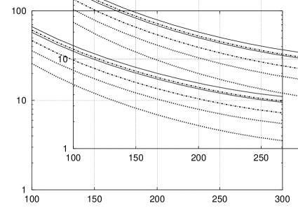
We demonstrate this behavior with two examples in Fig. 3, where we plot the production cross-sections for $m_{H}=115~{}{\rm GeV}$ and $m_{H}=275~{}{\rm GeV}$. We equate the renormalization and factorization scales and vary the factorization scale from $\mu=15~{}{\rm GeV}$ up to the mass of the Higgs boson. These plots illustrate that for smaller values of $\mu$, the NLO cross-section increases more rapidly than the NNLO cross-section, and the difference between the NLO and the NNLO results becomes smaller. Therefore, the convergence of the perturbative series is improved for smaller values of the factorization scale.

If we adopt this argument and restrict our analysis to small $\mu$ we find a Higgs production cross-section of $55\pm 5~{}{\rm pb}$ for $m_{H}=115~{}{\rm GeV}$, a somewhat larger value than obtained with the conventional scale choice $\mu=m_{H}$. It is interesting that recent studies [32] of the threshold resummed cross-section for Higgs boson production, matched to the NNLO calculation, detect a similar increase as compared to fixed order calculations with $\mu=m_{H}$.

VI Conclusions

In this paper, we have studied the Higgs boson production cross-section in hadron-hadron collisions. The main contribution to the hadronic cross-section originates from gluon-gluon fusion, which we have computed at NNLO (${\cal O}\left(\alpha_{s}^{4}\right)$) in perturbative QCD. The other partonic production channels, $qg\to H+X$, $q\bar{q}\to H+X$, $qq\to H+X$ and $qq^{\prime}\to H+X$, were also studied to order $\alpha_{s}^{4}$.

We have presented explicit analytic expressions for the partonic cross-sections valid within the heavy top-quark approximation. Finally, we have calculated the cross-section for direct Higgs boson production at the Tevatron and the LHC by performing a numerical convolution of the partonic cross-sections with the MRST 2002 NNLO set [30] of parton distribution functions. The residual scale dependence of the NNLO cross-section is approximately $\sim 15\%$ for the LHC and $\sim 23\%$ for the Tevatron. The NNLO $K$-factors are fairly large for both the LHC and the Tevatron. Nevertheless, the cross-section increases less from NLO to NNLO than from LO to NLO, indicating a slow convergence of the perturbative expansion.

While this calculation was in progress, Harlander and Kilgore [18] obtained an approximation of the partonic cross-sections by expanding around the Higgs boson production threshold. Our results for the partonic cross-sections are in complete agreement with their expansion. Also, we find a very good agreement of our numerical results for the NNLO Higgs production cross section with the results reported in [18].

In Section V, we have argued that it is more appropriate to choose smaller values of the factorization scale $\mu$ than the conventional choice $\mu=m_{H}$. Then, the NNLO corrections decrease, indicating a better convergence of the perturbative series. Moreover, with this choice, the fixed order results are in better agreement with recent estimates of the cross-section based on threshold resummation [32].

We have suggested a method for the algorithmic evaluation of inclusive phase-space integrals. This method combines the Cutkosky rules with integration-by-parts reduction algorithms to achieve a systematic reduction of phase-space integrals to a few master integrals. We have also shown how to compute these master integrals using differential equations produced with the IBP reduction algorithms.

The techniques discussed in this paper can be used to compute higher order corrections to other inclusive processes of direct phenomenological interest. We are also confident that this approach can be generalized to enable the calculation of differential distributions. In fact, a connection between phase-space integrals with a modified measure, such as the integrals that appear in the evaluation of invariant mass, energy and angular distributions, and loop integrals with unconventional propagators exists. This connection can be used to automate the calculation of differential distributions following the lines of Section III. The above ideas will be the subject of more detailed studies in future work.

Acknowledgments We would like to thank Robert Harlander and Bill Kilgore for comparisons with their results of Ref. [18]. We are grateful to Frank Petriello for careful reading of the manuscript and invaluable suggestions. This research was supported by the DOE under grant number DE-AC03-76SF00515.

Appendix

In this Appendix, some formulae used in our calculation are given.

A Splitting functions

We first summarize the formulae for the space-like splitting functions.

$\displaystyle P_{gg}^{(0)}=\left(\frac{11}{4}-\frac{1}{6}n_{f}\right)\delta(1-x)+3\left(x(1-x)+\frac{(1-x)}{x}-1\right)+3\left[\frac{1}{1-x}\right]_{+},$ (120)
$\displaystyle P^{(0)}_{gq}=\frac{2}{3}\frac{(1+(1-x)^{2})}{x},$ (121)
$\displaystyle P^{(0)}_{qg}=\frac{1}{4}\left(x^{2}+(1-x)^{2}\right),$ (122)
$\displaystyle P^{(0)}_{qq}=\frac{2}{3}\left(\frac{3}{2}\delta(1-x)-1-x+2\left[\frac{1}{1-x}\right]_{+}\right),$ (123)
$\displaystyle P^{(1)}_{gg}=\left(6+\frac{27}{4}\zeta_{3}\right)\delta(1-x)+\left(\frac{67}{4}-\frac{9}{2}\zeta_{2}\right)\left[\frac{1}{1-x}\right]_{+}+\frac{9(x^{2}+x+1)^{2}}{x(1+x)}{\rm Li}_{2}(-x)$ (124)
$\displaystyle+\frac{9(3+2x^{2}+4x+2x^{3})\zeta_{2}}{2(1+x)}+\frac{9(x^{2}-x-1)^{2}}{2(1-x^{2})}\ln^{2}x-\frac{25}{8}-\frac{109x}{8}$ (125)
$\displaystyle+\left(\frac{9(x^{2}+x+1)^{2}}{x(1+x)}\ln(1+x)-\frac{9(x^{2}-x+1)^{2}}{x(1-x)}\ln(1-x)-\frac{75}{4}+\frac{33}{4}x-33x^{2}\right)\ln(x)$ (126)
$\displaystyle+n_{f}\left[-\frac{2}{3}\delta(1-x)-\frac{5}{6}\left[\frac{1}{1-x}\right]_{+}-\frac{1+x}{3}\ln^{2}(x)-\left(\frac{3}{2}+\frac{13x}{6}\right)\ln(x)+\frac{(-9x-9x^{2}+109x^{3}-61)}{36x}\right],$ (127)
$\displaystyle P^{(1)}_{gq}=\frac{9x+23x^{2}+9+44x^{3}}{9x}-\frac{4n_{f}(4x^{2}+5-5x)}{27x}+\frac{2(2+2x+x^{2}){\rm Li}_{2}\left(-x\right)}{x}+4\zeta_{2}$ (128)
$\displaystyle+\frac{5(2-2x+x^{2})\log^{2}(1-x)}{9x}+\log(x)\left(\frac{2(2+2x+x^{2})\log(1+x)}{x}-\frac{100}{9}-\frac{31x}{9}-\frac{8x^{2}}{3}\right)$ (129)
$\displaystyle+\log(1-x)\left(-\frac{2(2-2x+x^{2})}{x}(\log(x)+\frac{n_{f}}{9})+\frac{31x^{2}+42-42x}{9x}\right)+\frac{(14+11x)\log^{2}(x)}{9}.$ (130)

B Master Integrals

Below we list the master integrals required in this calculation. We denote $\hat{s}=p_{12}^{2}=(p_{1}+p_{2})^{2}$, $z=m_{H}^{2}/\hat{s}$ and for simplicity we set $\hat{s}=1$.

1 Double-Virtual

The master integrals for the double-virtual corrections can be expressed in terms of Gamma functions with the exception of the cross-triangle which has been calculated in [33]. For completeness, we list their $\epsilon$-expansion below:

\Text(5,10)[]$p_{2}$\Text(5,50)[]$p_{1}$\ArrowLine(10,10)(20, 10) \ArrowLine(10,50)(20,50) \Line(20,10)(60,30) \Line(20,50)(60,30) \Line(20,50)(40,20) \Line(20,10)(40,40) \DashLine(70,40)(70,20)4 \SetWidth2 \Line(60,30)(80,30) $\displaystyle\equiv$ $\displaystyle\int\frac{d^{d}k}{i\pi^{\frac{d}{2}}}\frac{d^{d}l}{i\pi^{\frac{d}{2}}}\frac{\delta(p_{12}^{2}-m_{H}^{2})}{k^{2}(k+p_{12})^{2}(l+p_{12})^{2}(l+p_{1})^{2}(k-l-p_{1})^{2}(k-l)^{2}}$ (131)
$\displaystyle=$ $\displaystyle\delta\left(1-z\right)\Gamma\left(1+\epsilon\right)^{2}{\rm Re}\left(e^{-2i\pi\epsilon}\right)\left[\frac{1}{{\epsilon}^{4}}-\,{\frac{7\zeta_{2}}{{\epsilon}^{2}}}-27\,{\frac{\zeta_{3}}{\epsilon}}-{\frac{19}{60}}\,{\pi}^{4}+{\cal O}(\epsilon)\right],$ (133)

\Text(5,10)[]$p_{2}$\Text(5,50)[]$p_{1}$\ArrowLine(10,10)(20, 10) \ArrowLine(10,50)(20,50) \Line(20,10)(60,30) \Line(20,50)(60,30) \DashLine(70,40)(70,20)4 \Oval(20,30)(20,8)(0) \SetWidth2 \Line(60,30)(80,30) $\displaystyle\equiv$ $\displaystyle\int\frac{d^{d}k}{i\pi^{\frac{d}{2}}}\frac{d^{d}l}{i\pi^{\frac{d}{2}}}\frac{\delta(p_{12}^{2}-m_{H}^{2})}{k^{2}(k+p_{12})^{2}(l+p_{12})^{2}(k-l)^{2}}$ (137)
$\displaystyle=\delta\left(1-z\right)\Gamma\left(1+\epsilon\right)^{2}{\rm Re}\left(e^{-2i\pi\epsilon}\right)\frac{1}{2}\Bigg{[}\frac{1}{\epsilon^{2}}+\frac{5}{\epsilon}+19+\left(65-8\zeta_{3}\right)\epsilon$
$\displaystyle+\left(211-40\zeta_{3}-\frac{2\pi^{4}}{15}\right)\epsilon^{2}+{\cal O}(\epsilon^{3})\Bigg{]},$

\Text(5,20)[]$p_{2}$\Text(5,40)[]$p_{1}$\ArrowLine(10,20)(20, 30) \ArrowLine(10,40)(20,30) \Line(20,30)(60,30) \CArc(40,30)(20,0,360) \DashLine(67,40)(67,20)4 \SetWidth2 \Line(60,30)(74,30) $\displaystyle\equiv$ $\displaystyle\int\frac{d^{d}k}{i\pi^{\frac{d}{2}}}\frac{d^{d}l}{i\pi^{\frac{d}{2}}}\frac{\delta(p_{12}^{2}-m_{H}^{2})}{k^{2}(l+p_{12})^{2}(k-l)^{2}}$ (141)
$\displaystyle=\delta\left(1-z\right)\Gamma\left(1+\epsilon\right)^{2}{\rm Re}\left(e^{-2i\pi\epsilon}\right)\frac{1}{2}\Bigg{[}-\frac{1}{4\epsilon}-\frac{13}{8}+\left(\frac{\zeta_{2}}{2}-\frac{115}{16}\right)\epsilon$
$\displaystyle+\left(\frac{5\zeta_{3}}{2}-\frac{865}{32}+\frac{13\zeta_{2}}{4}\right)\epsilon^{2}+\left(-\frac{5971}{64}+\frac{115\zeta_{2}}{8}+\frac{65\zeta_{3}}{4}+\frac{11\zeta_{2}^{2}}{10}\right)\epsilon^{3}+{\cal O}(\epsilon^{4})\Bigg{]},$

\Text(5,20)[]$p_{2}$\Text(5,40)[]$p_{1}$\ArrowLine(10,20)(20, 30) \ArrowLine(10,40)(20,30) \CArc(30,30)(10,0,360) \CArc(50,30)(10,0,360) \DashLine(70,40)(70,20)4 \SetWidth2 \Line(60,30)(80,30) $\displaystyle=$ $\displaystyle\delta(p_{12}^{2}-m_{H}^{2})\left[\int\frac{d^{d}k}{i\pi^{\frac{d}{2}}}\frac{1}{k^{2}(k+p_{12})^{2}}\right]^{2}$ (145)
$\displaystyle=\delta\left(1-z\right)\Gamma\left(1+\epsilon\right)^{2}{\rm Re}\left(e^{-2i\pi\epsilon}\right)\Bigg{[}\frac{1}{\epsilon^{2}}+\frac{4}{\epsilon}+12-2\zeta_{2}+\left(32-8\zeta_{2}-4\zeta_{3}\right)\epsilon+$
$\displaystyle+\left(80-16\zeta_{3}-24\zeta_{2}-\frac{4\zeta_{2}^{2}}{5}\right)\epsilon^{2}+{\cal O}(\epsilon^{3})\Bigg{]},$

\Text(5,20)[]$p_{2}$\Text(5,40)[]$p_{1}$\Text(87,20)[]$p_{2}$\Text(87,40)[]$p_{1}$\ArrowLine(70,30)(80, 40) \ArrowLine(70,30)(80,20) \ArrowLine(10,20)(20, 30) \ArrowLine(10,40)(20,30) \CArc(30,30)(10,0,360) \CArc(60,30)(10,0,360) \DashLine(45,40)(45,20)4 \SetWidth2 \Line(40,30)(50,30) $\displaystyle=$ $\displaystyle\delta(p_{12}^{2}-m_{H}^{2})\left|\int\frac{d^{d}k}{i\pi^{\frac{d}{2}}}\frac{1}{k^{2}(k+p_{12})^{2}}\right|^{2}$ (149)
$\displaystyle=\delta\left(1-z\right)\Gamma\left(1+\epsilon\right)^{2}\Bigg{[}\frac{1}{\epsilon^{2}}+\frac{4}{\epsilon}+12-2\zeta_{2}+\left(32-8\zeta_{2}-4\zeta_{3}\right)\epsilon+$
$\displaystyle+\left(80-16\zeta_{3}-24\zeta_{2}-\frac{4\zeta_{2}^{2}}{5}\right)\epsilon^{2}+{\cal O}(\epsilon^{3})\Bigg{]}.$

2 Real-Virtual

For the real-virtual contributions we find six master integrals:

\Text(5,20)[]p2\Text(5,40)[]p1\Text(75,20)[]p2\Text(75,40)[]p1\ArrowLine(10,20)(20, 30) \ArrowLine(10,40)(20,30) \ArrowLine(60,30)(70,40) \ArrowLine(60,30)(70,20) \CArc(30,30)(10,180,360) \CArc(50,30)(10,0,360) \DashLine(30,50)(30,10)4 \SetWidth2 \CArc(30,30)(10,0,180) =ddkiπd2ddlδ(k2mH2)δ((k+p12)2)l2(l+p12)2\Text(5,20)[]p2\Text(5,40)[]p1\Text(75,20)[]p2\Text(75,40)[]p1\ArrowLine(10,20)(20, 30) \ArrowLine(10,40)(20,30) \ArrowLine(60,30)(70,40) \ArrowLine(60,30)(70,20) \CArc(30,30)(10,180,360) \CArc(50,30)(10,0,360) \DashLine(30,50)(30,10)4 \SetWidth2 \CArc(30,30)(10,0,180) superscript𝑑𝑑𝑘𝑖superscript𝜋𝑑2superscript𝑑𝑑𝑙𝛿superscript𝑘2superscriptsubscript𝑚𝐻2𝛿superscript𝑘subscript𝑝122superscript𝑙2superscript𝑙subscript𝑝122\displaystyle\begin{picture}(80.0,60.0)(0.0,27.0)\Text(5,20)[]{$p_{2}$} \Text(5,40)[]{$p_{1}$} \Text(75,20)[]{$p_{2}$} \Text(75,40)[]{$p_{1}$} \ArrowLine(10,20)(20, 30) \ArrowLine(10,40)(20,30) \ArrowLine(60,30)(70,40) \ArrowLine(60,30)(70,20) \CArc(30,30)(10,180,360) \CArc(50,30)(10,0,360) \DashLine(30,50)(30,10){4} \SetWidth{2} \CArc(30,30)(10,0,180) \end{picture}=\int\frac{d^{d}k}{i\pi^{\frac{d}{2}}}d^{d}l\frac{\delta\left(k^{2}-m_{H}^{2}\right)\delta\left((k+p_{12})^{2}\right)}{l^{2}(l+p_{12})^{2}} (150)
(151)
(152)
$\displaystyle={\cal P}{\cal L}{\rm Re}\left(e^{-i\pi\epsilon}\right)s^{-2\epsilon}(1-z)^{1-2\epsilon},$ (153)

\Text(5,20)[]p2\Text(5,40)[]p1\Text(73,10)[]p2\Text(73,50)[]p1\ArrowLine(10,20)(20, 30) \ArrowLine(10,40)(20,30) \ArrowLine(55,50)(65,50) \ArrowLine(55,10)(65,10) \Line(20,30)(55,10) \Oval(55,30)(20,5)(0) \DashLine(37.5,50)(37.5,10)4 \SetWidth2 \Line(20, 30)(55, 50) =ddkiπd2ddlδ(k2mH2)δ((k+p12)2)(kl)2(l+p1)2\Text(5,20)[]p2\Text(5,40)[]p1\Text(73,10)[]p2\Text(73,50)[]p1\ArrowLine(10,20)(20, 30) \ArrowLine(10,40)(20,30) \ArrowLine(55,50)(65,50) \ArrowLine(55,10)(65,10) \Line(20,30)(55,10) \Oval(55,30)(20,5)(0) \DashLine(37.5,50)(37.5,10)4 \SetWidth2 \Line(20, 30)(55, 50) superscript𝑑𝑑𝑘𝑖superscript𝜋𝑑2superscript𝑑𝑑𝑙𝛿superscript𝑘2superscriptsubscript𝑚𝐻2𝛿superscript𝑘subscript𝑝122superscript𝑘𝑙2superscript𝑙subscript𝑝12\displaystyle\begin{picture}(80.0,60.0)(0.0,27.0)\Text(5,20)[]{$p_{2}$} \Text(5,40)[]{$p_{1}$} \Text(73,10)[]{$p_{2}$} \Text(73,50)[]{$p_{1}$} \ArrowLine(10,20)(20, 30) \ArrowLine(10,40)(20,30) \ArrowLine(55,50)(65,50) \ArrowLine(55,10)(65,10) \Line(20,30)(55,10) \Oval(55,30)(20,5)(0) \DashLine(37.5,50)(37.5,10){4} \SetWidth{2} \Line(20, 30)(55, 50) \end{picture}=\int\frac{d^{d}k}{i\pi^{\frac{d}{2}}}d^{d}l\frac{\delta\left(k^{2}-m_{H}^{2}\right)\delta\left((k+p_{12})^{2}\right)}{(k-l)^{2}(l+p_{1})^{2}} (154)
(155)
(156)
$\displaystyle={\cal P}{\cal L}s^{-2\epsilon}\frac{1-2\epsilon}{1-3\epsilon}\frac{\Gamma(1-2\epsilon)^{2}}{\Gamma(1-\epsilon)\Gamma(1-3\epsilon)}(1-z)^{1-3\epsilon},$ (157)

\Text(5,20)[]p2\Text(5,40)[]p1\Text(73,20)[]p2\Text(73,40)[]p1\ArrowLine(10,20)(20, 30) \ArrowLine(10,40)(20,30) \ArrowLine(55,30)(65,40) \ArrowLine(55,30)(65,20) \CArc(37.5, 30)(17.5, 180, 450) \CArc(55,47.5)(17.5,180,270) \DashLine(32.5,50)(32.5,10)4 \SetWidth2 \CArc(37.5, 30)(17.5, 90, 180) =ddkiπd2ddlδ(k2mH2)δ((k+p12)2)(kl)2l2\Text(5,20)[]p2\Text(5,40)[]p1\Text(73,20)[]p2\Text(73,40)[]p1\ArrowLine(10,20)(20, 30) \ArrowLine(10,40)(20,30) \ArrowLine(55,30)(65,40) \ArrowLine(55,30)(65,20) \CArc(37.5, 30)(17.5, 180, 450) \CArc(55,47.5)(17.5,180,270) \DashLine(32.5,50)(32.5,10)4 \SetWidth2 \CArc(37.5, 30)(17.5, 90, 180) superscript𝑑𝑑𝑘𝑖superscript𝜋𝑑2superscript𝑑𝑑𝑙𝛿superscript𝑘2superscriptsubscript𝑚𝐻2𝛿superscript𝑘subscript𝑝122superscript𝑘𝑙2superscript𝑙2\displaystyle\begin{picture}(80.0,60.0)(0.0,27.0)\Text(5,20)[]{$p_{2}$} \Text(5,40)[]{$p_{1}$} \Text(73,20)[]{$p_{2}$} \Text(73,40)[]{$p_{1}$} \ArrowLine(10,20)(20, 30) \ArrowLine(10,40)(20,30) \ArrowLine(55,30)(65,40) \ArrowLine(55,30)(65,20) \CArc(37.5, 30)(17.5, 180, 450) \CArc(55,47.5)(17.5,180,270) \DashLine(32.5,50)(32.5,10){4} \SetWidth{2} \CArc(37.5, 30)(17.5, 90, 180) \end{picture}=\int\frac{d^{d}k}{i\pi^{\frac{d}{2}}}d^{d}l\frac{\delta\left(k^{2}-m_{H}^{2}\right)\delta\left((k+p_{12})^{2}\right)}{(k-l)^{2}l^{2}} (158)
(159)
(160)
$\displaystyle={\cal P}{\cal L}s^{-2\epsilon}{\rm Re}\left(e^{-i\pi\epsilon}\right)z^{-\epsilon}(1-z)^{1-2\epsilon},$ (161)

\Text(5,20)[]p2\Text(5,40)[]p1\Text(73,10)[]p2\Text(73,50)[]p1\ArrowLine(10,20)(20, 30) \ArrowLine(10,40)(20,30) \ArrowLine(55,50)(65,50) \ArrowLine(55,10)(65,10) \Line(20,30)(55,10) \Line(45,44.28)(55,50) \Line(45,44.28)(55,10) \Line(55,50)(55,10) \DashLine(37.5,50)(37.5,10)4 \SetWidth2 \Line(20, 30)(45, 44.28) =ddkiπd2ddlδ(k2mH2)δ((k+p12)2)(kl)2(l+p1)2l2,\Text(5,20)[]p2\Text(5,40)[]p1\Text(73,10)[]p2\Text(73,50)[]p1\ArrowLine(10,20)(20, 30) \ArrowLine(10,40)(20,30) \ArrowLine(55,50)(65,50) \ArrowLine(55,10)(65,10) \Line(20,30)(55,10) \Line(45,44.28)(55,50) \Line(45,44.28)(55,10) \Line(55,50)(55,10) \DashLine(37.5,50)(37.5,10)4 \SetWidth2 \Line(20, 30)(45, 44.28) superscript𝑑𝑑𝑘𝑖superscript𝜋𝑑2superscript𝑑𝑑𝑙𝛿superscript𝑘2superscriptsubscript𝑚𝐻2𝛿superscript𝑘subscript𝑝122superscript𝑘𝑙2superscript𝑙subscript𝑝12superscript𝑙2\displaystyle\begin{picture}(80.0,60.0)(0.0,27.0)\Text(5,20)[]{$p_{2}$} \Text(5,40)[]{$p_{1}$} \Text(73,10)[]{$p_{2}$} \Text(73,50)[]{$p_{1}$} \ArrowLine(10,20)(20, 30) \ArrowLine(10,40)(20,30) \ArrowLine(55,50)(65,50) \ArrowLine(55,10)(65,10) \Line(20,30)(55,10) \Line(45,44.28)(55,50) \Line(45,44.28)(55,10) \Line(55,50)(55,10) \DashLine(37.5,50)(37.5,10){4} \SetWidth{2} \Line(20, 30)(45, 44.28) \end{picture}=\int\frac{d^{d}k}{i\pi^{\frac{d}{2}}}d^{d}l\frac{\delta\left(k^{2}-m_{H}^{2}\right)\delta\left((k+p_{12})^{2}\right)}{(k-l)^{2}(l+p_{1})^{2}l^{2}}, (162)
(163)
(164)
$\displaystyle={\cal P}\Gamma(1+\epsilon)\frac{z^{-2\epsilon}}{1-2\epsilon}\Bigg{\{}\frac{1}{\epsilon}\left[{\rm Li}_{2}\left(z\right)+\frac{\log^{2}(z)}{2}-\zeta_{2}\right]+5{\rm S}_{12}\left(z\right)$ (165)
$\displaystyle-4{\rm Li}_{3}\left(z\right)+4\log(z){\rm Li}_{2}\left(z\right)+\frac{\log^{3}(z)}{2}+2\zeta_{2}\log(z)-\zeta_{3}$ (166)
$\displaystyle+{\cal O}\left(\epsilon\right)\Bigg{\}},$ (167)

\Text(5,10)[]p2\Text(5,50)[]p1\Text(73,10)[]p1\Text(73,50)[]p2\ArrowLine(10,50)(20, 50) \ArrowLine(10,10)(20,10) \ArrowLine(55,50)(65,50) \ArrowLine(55,10)(65,10) \Line(20,10)(55,10) \Line(55,50)(55,10) \Line(37.5,50)(37.5,10) \Line(20,50)(20,10) \Line(35, 50)(55, 50) \DashLine(28.25,55)(28.25,5)4 \SetWidth2 \Line(20, 50)(37.5, 50) =ddkiπd2ddlδ(k2mH2)δ((k+p12)2)(k+p1)2(l+p12)2(l+p2)2l2(kl)2,\Text(5,10)[]p2\Text(5,50)[]p1\Text(73,10)[]p1\Text(73,50)[]p2\ArrowLine(10,50)(20, 50) \ArrowLine(10,10)(20,10) \ArrowLine(55,50)(65,50) \ArrowLine(55,10)(65,10) \Line(20,10)(55,10) \Line(55,50)(55,10) \Line(37.5,50)(37.5,10) \Line(20,50)(20,10) \Line(35, 50)(55, 50) \DashLine(28.25,55)(28.25,5)4 \SetWidth2 \Line(20, 50)(37.5, 50) superscript𝑑𝑑𝑘𝑖superscript𝜋𝑑2superscript𝑑𝑑𝑙𝛿superscript𝑘2superscriptsubscript𝑚𝐻2𝛿superscript𝑘subscript𝑝122superscript𝑘subscript𝑝12superscript𝑙subscript𝑝122superscript𝑙subscript𝑝22superscript𝑙2superscript𝑘𝑙2\displaystyle\begin{picture}(80.0,60.0)(0.0,27.0)\Text(5,10)[]{$p_{2}$} \Text(5,50)[]{$p_{1}$} \Text(73,10)[]{$p_{1}$} \Text(73,50)[]{$p_{2}$} \ArrowLine(10,50)(20, 50) \ArrowLine(10,10)(20,10) \ArrowLine(55,50)(65,50) \ArrowLine(55,10)(65,10) \Line(20,10)(55,10) \Line(55,50)(55,10) \Line(37.5,50)(37.5,10) \Line(20,50)(20,10) \Line(35, 50)(55, 50) \DashLine(28.25,55)(28.25,5){4} \SetWidth{2} \Line(20, 50)(37.5, 50) \end{picture}=\int\frac{d^{d}k}{i\pi^{\frac{d}{2}}}d^{d}l\frac{\delta\left(k^{2}-m_{H}^{2}\right)\delta\left((k+p_{12})^{2}\right)}{(k+p_{1})^{2}(l+p_{12})^{2}(l+p_{2})^{2}l^{2}(k-l)^{2}}, (168)
(169)
(170)
$\displaystyle=-{\cal P}\frac{\Gamma(1+\epsilon)}{3(1-2\epsilon)}\Bigg{\{}(1-z)^{1-3\epsilon}\left[\frac{1}{\epsilon^{3}}-\frac{2\zeta_{2}}{\epsilon}-6\zeta_{3}-11\zeta_{4}\epsilon+{\cal O}\left(\epsilon^{2}\right)\right]$ (171)
$\displaystyle+(1-z)^{1-2\epsilon}\left[\frac{\log(z)}{\epsilon^{2}}+\frac{{\rm Li}_{2}\left(z\right)-\log^{2}(z)-\zeta_{2}}{3\epsilon}\right.$ (172)
$\displaystyle\left.+\frac{{\rm S}_{12}\left(z\right)-2{\rm Li}_{3}\left(z\right)-8\zeta_{2}\log(z)+\zeta_{3}}{3}+{\cal O}\left(\epsilon\right)\right]\Bigg{\}},$ (173)

\Text(5,20)[]p2\Text(5,40)[]p1\Text(73,10)[]p2\Text(73,50)[]p1\ArrowLine(10,20)(20, 30) \ArrowLine(10,40)(20,30) \ArrowLine(55,50)(65,50) \ArrowLine(55,10)(65,10) \Line(20,30)(55,10) \Line(45,44.28)(55,50) \Line(45,44.28)(55,10) \Line(55,50)(45,16.72) \DashLine(37.5,50)(37.5,10)4 \SetWidth2 \Line(20, 30)(45, 44.28) =ddkiπd2ddlδ(k2mH2)δ((k+p12)2)(l+p12)2(l+p1)2(klp1)2(kl)2\Text(5,20)[]p2\Text(5,40)[]p1\Text(73,10)[]p2\Text(73,50)[]p1\ArrowLine(10,20)(20, 30) \ArrowLine(10,40)(20,30) \ArrowLine(55,50)(65,50) \ArrowLine(55,10)(65,10) \Line(20,30)(55,10) \Line(45,44.28)(55,50) \Line(45,44.28)(55,10) \Line(55,50)(45,16.72) \DashLine(37.5,50)(37.5,10)4 \SetWidth2 \Line(20, 30)(45, 44.28) superscript𝑑𝑑𝑘𝑖superscript𝜋𝑑2superscript𝑑𝑑𝑙𝛿superscript𝑘2superscriptsubscript𝑚𝐻2𝛿superscript𝑘subscript𝑝122superscript𝑙subscript𝑝122superscript𝑙subscript𝑝12superscript𝑘𝑙subscript𝑝12superscript𝑘𝑙2\displaystyle\begin{picture}(80.0,60.0)(0.0,27.0)\Text(5,20)[]{$p_{2}$} \Text(5,40)[]{$p_{1}$} \Text(73,10)[]{$p_{2}$} \Text(73,50)[]{$p_{1}$} \ArrowLine(10,20)(20, 30) \ArrowLine(10,40)(20,30) \ArrowLine(55,50)(65,50) \ArrowLine(55,10)(65,10) \Line(20,30)(55,10) \Line(45,44.28)(55,50) \Line(45,44.28)(55,10) \Line(55,50)(45,16.72) \DashLine(37.5,50)(37.5,10){4} \SetWidth{2} \Line(20, 30)(45, 44.28) \end{picture}=\int\frac{d^{d}k}{i\pi^{\frac{d}{2}}}d^{d}l\frac{\delta\left(k^{2}-m_{H}^{2}\right)\delta\left((k+p_{12})^{2}\right)}{(l+p_{12})^{2}(l+p_{1})^{2}(k-l-p_{1})^{2}(k-l)^{2}} (174)
(175)
(176)
$\displaystyle=-2{\cal P}\frac{\Gamma(1+\epsilon)}{1-2\epsilon}(1-z)^{-1-4\epsilon}\Bigg{\{}\left[\frac{1}{\epsilon^{3}}-\frac{6\zeta_{2}}{\epsilon}-16\zeta_{3}-18\zeta_{4}\epsilon+{\cal O}\left(\epsilon^{2}\right)\right].$ (177)
$\displaystyle+\left[\frac{\log(z)}{\epsilon^{2}}-\frac{{\rm Li}_{2}\left(z\right)-\zeta_{2}}{\epsilon}+{\rm S}_{12}\left(z\right)-2{\rm Li}_{3}\left(z\right)-\frac{\log^{3}(z)}{3}+\zeta_{3}+{\cal O}\left(\epsilon\right)\right]\Bigg{\}},$ (178)

where the common factors ${\cal P}$ and ${\cal L}$ are:

$${\cal P}=\frac{\pi^{\frac{3}{2}-\epsilon}}{2^{3-2\epsilon}\Gamma(\frac{3}{2}-\epsilon)}$$ (179)

and

$${\cal L}=\frac{\Gamma(\epsilon)\Gamma(1-\epsilon)^{2}}{\Gamma(2-2\epsilon)}.$$ (180)

3 Double-Real

We find the following master integrals for the double-real contributions:

\Text(5,20)[]p2\Text(5,40)[]p1\Text(77,20)[]p2\Text(77,40)[]p1\Line(10,20)(20, 30) \Line(10,40)(20,30) \Line(60,30)(70,40) \Line(60,30)(70,20) \CArc(40,30)(20,0,360) \DashLine(40,55)(40,5)4 \SetWidth2 \Line(20, 30)(60, 30) ddkddlδ((kl)2mH2)δ((l+p1+p2)2)δ(k2)\Text(5,20)[]p2\Text(5,40)[]p1\Text(77,20)[]p2\Text(77,40)[]p1\Line(10,20)(20, 30) \Line(10,40)(20,30) \Line(60,30)(70,40) \Line(60,30)(70,20) \CArc(40,30)(20,0,360) \DashLine(40,55)(40,5)4 \SetWidth2 \Line(20, 30)(60, 30) superscript𝑑𝑑𝑘superscript𝑑𝑑𝑙𝛿superscript𝑘𝑙2superscriptsubscript𝑚𝐻2𝛿superscript𝑙subscript𝑝1subscript𝑝22𝛿superscript𝑘2\displaystyle\begin{picture}(80.0,60.0)(0.0,27.0)\Text(5,20)[]{$p_{2}$} \Text(5,40)[]{$p_{1}$} \Text(77,20)[]{$p_{2}$} \Text(77,40)[]{$p_{1}$} \Line(10,20)(20, 30) \Line(10,40)(20,30) \Line(60,30)(70,40) \Line(60,30)(70,20) \CArc(40,30)(20,0,360) \DashLine(40,55)(40,5){4} \SetWidth{2} \Line(20, 30)(60, 30) \end{picture}\equiv\int d^{d}kd^{d}l\delta((k-l)^{2}-m_{H}^{2})\delta((l+p_{1}+p_{2})^{2})\delta(k^{2}) (181)
(182)
(183)
$\displaystyle=\frac{{\cal P}^{2}\Gamma(1-2\epsilon)^{2}}{\Gamma(1-4\epsilon)}\Bigg{\{}\frac{1-2\epsilon}{2(3-4\epsilon)(1-4\epsilon)}(1-z)^{3-4\epsilon}+(1-z)^{-4\epsilon}\Bigg{[}-\frac{1}{6}(1-z)\left(z^{2}-5z-2\right)+z\log(z)$ (184)
$\displaystyle-\epsilon\left(\frac{5}{36}(1-z)(4z^{2}-17z-5)+\frac{z(z+2)}{2}\log(z)+\frac{z\log(z)^{2}}{2}+4z{\rm Li}_{2}\left(1-z\right)\right)$ (185)
$\displaystyle+\epsilon^{2}\left(8z{\rm S}_{12}\left(1-z\right)-16z{\rm Li}_{3}\left(1-z\right)+\frac{z\log(z)^{3}}{6}+\frac{56z^{3}}{27}+\frac{z(2+z)}{4}\log(z)^{2}\right.$ (186)
$\displaystyle\left.-\frac{691}{72}z^{2}+\frac{56z}{9}+\left(z^{2}+4z+1\right){\rm Li}_{2}\left(1-z\right)+\left(6{\rm Li}_{2}\left(1-z\right)-\frac{5z+8}{4}\right)z\log(z)\right.$ (187)
$\displaystyle\left.+\frac{281}{216}\right)+{\cal O}\left(\epsilon^{3}\right)\Bigg{]}\Bigg{\}},$ (188)
\Text(5,20)[]p2\Text(5,40)[]p1\Text(73,20)[]p2\Text(73,40)[]p1\Line(10,20)(20, 30) \Line(10,40)(20,30) \Line(55,30)(65,40) \Line(55,30)(65,20) \DashCArc(37.5, 30)(17.5, 90, 180)1.5 \CArc(37.5, 30)(17.5, 180, 450) \DashLine(44.5,50)(44.5,10)4 \SetWidth2 \CArc(55,47.5)(17.5,180,270) ddkddlδ((kl)2mH2)δ((l+p1+p2)2)δ(k2)l2\Text(5,20)[]p2\Text(5,40)[]p1\Text(73,20)[]p2\Text(73,40)[]p1\Line(10,20)(20, 30) \Line(10,40)(20,30) \Line(55,30)(65,40) \Line(55,30)(65,20) \DashCArc(37.5, 30)(17.5, 90, 180)1.5 \CArc(37.5, 30)(17.5, 180, 450) \DashLine(44.5,50)(44.5,10)4 \SetWidth2 \CArc(55,47.5)(17.5,180,270) superscript𝑑𝑑𝑘superscript𝑑𝑑𝑙𝛿superscript𝑘𝑙2superscriptsubscript𝑚𝐻2𝛿superscript𝑙subscript𝑝1subscript𝑝22𝛿superscript𝑘2superscript𝑙2\displaystyle\begin{picture}(80.0,60.0)(0.0,27.0)\Text(5,20)[]{$p_{2}$} \Text(5,40)[]{$p_{1}$} \Text(73,20)[]{$p_{2}$} \Text(73,40)[]{$p_{1}$} \Line(10,20)(20, 30) \Line(10,40)(20,30) \Line(55,30)(65,40) \Line(55,30)(65,20) \DashCArc(37.5, 30)(17.5, 90, 180){1.5} \CArc(37.5, 30)(17.5, 180, 450) \DashLine(44.5,50)(44.5,10){4} \SetWidth{2} \CArc(55,47.5)(17.5,180,270) \end{picture}\equiv\int d^{d}kd^{d}l\delta((k-l)^{2}-m_{H}^{2})\delta((l+p_{1}+p_{2})^{2})\delta(k^{2})l^{2} (189)
(190)
(191)
$\displaystyle=\frac{{\cal P}^{2}\Gamma(1-2\epsilon)^{2}}{\Gamma(1-4\epsilon)}(1-z)^{-4\epsilon}\Bigg{\{}(1-z)^{3}+\epsilon\left[(3-z)z^{2}\log(z)\right.$ (192)
$\displaystyle\left.+\frac{1}{2}(1-z)(5z^{2}-6z+5)\right]+\epsilon^{2}\left[\frac{1}{2}(z-3)z^{2}\log(z)^{2}-\frac{1}{2}(5z^{2}-7z+4)z\log(z)\right.$ (193)
$\displaystyle\left.+2(z+1)(z^{2}-4z+1){\rm Li}_{2}\left(1-z\right)+\frac{1}{4}(1-z)(27z^{2}-26z+27)\right]$ (194)
$\displaystyle+\epsilon^{3}\left[-\frac{1}{6}(z-3)z^{2}\log^{3}(z)-6(z-3)z^{2}{\rm Li}_{2}\left(1-z\right)\log(z)+\frac{1}{4}z(5z^{2}-7z+4)\log^{2}(z)\right.$ (195)
$\displaystyle\left.-\frac{1}{4}(27z^{2}-25z+28)z\log(z)+(1+z)(5z^{2}-8z+5){\rm Li}_{2}\left(1-z\right)\right.$ (196)
$\displaystyle\left.+8(1+z)(z^{2}-4z+1){\rm Li}_{3}\left(1-z\right)+(-10z^{3}+30z^{2}-6z+2){\rm S}_{12}\left(1-z\right)\right.$ (197)
$\displaystyle\left.+\frac{1}{8}(1-z)(153z^{2}-142z+153)\right]+{\cal O}\left(\epsilon^{4}\right)\Bigg{\}},$ (198)
\Text(5,20)[]p2\Text(5,40)[]p1\Text(73,20)[]p2\Text(73,40)[]p1\Line(10,20)(20, 30) \Line(10,40)(20,30) \Line(55,30)(65,40) \Line(55,30)(65,20) \CArc(37.5, 30)(17.5, 0, 360) \DashLine(30,50)(45,10)4 \SetWidth2 \Line(37.5, 47.50)(37.5,12.50) ddkddlδ((kl)2mH2)δ((l+p1+p2)2)δ(k2)l2(k+p1+p2)2\Text(5,20)[]p2\Text(5,40)[]p1\Text(73,20)[]p2\Text(73,40)[]p1\Line(10,20)(20, 30) \Line(10,40)(20,30) \Line(55,30)(65,40) \Line(55,30)(65,20) \CArc(37.5, 30)(17.5, 0, 360) \DashLine(30,50)(45,10)4 \SetWidth2 \Line(37.5, 47.50)(37.5,12.50) superscript𝑑𝑑𝑘superscript𝑑𝑑𝑙𝛿superscript𝑘𝑙2superscriptsubscript𝑚𝐻2𝛿superscript𝑙subscript𝑝1subscript𝑝22𝛿superscript𝑘2superscript𝑙2superscript𝑘subscript𝑝1subscript𝑝22\displaystyle\begin{picture}(80.0,60.0)(0.0,27.0)\Text(5,20)[]{$p_{2}$} \Text(5,40)[]{$p_{1}$} \Text(73,20)[]{$p_{2}$} \Text(73,40)[]{$p_{1}$} \Line(10,20)(20, 30) \Line(10,40)(20,30) \Line(55,30)(65,40) \Line(55,30)(65,20) \CArc(37.5, 30)(17.5, 0, 360) \DashLine(30,50)(45,10){4} \SetWidth{2} \Line(37.5, 47.50)(37.5,12.50) \end{picture}\equiv\int d^{d}kd^{d}l\frac{\delta((k-l)^{2}-m_{H}^{2})\delta((l+p_{1}+p_{2})^{2})\delta(k^{2})}{l^{2}(k+p_{1}+p_{2})^{2}} (199)
(200)
(201)
$\displaystyle={\cal P}^{2}z^{-\epsilon}(1+z)^{-\epsilon}\Bigg{\{}-2{\rm Li}_{2}\left(-z\right)-\zeta_{2}+\frac{\log(z)}{2}\left(\log(z)-4\log(1+z)\right)$ (202)
$\displaystyle+\epsilon\left[-8\log(1+z){\rm Li}_{2}\left(z\right)+\frac{\log(z)}{6}\left(\log^{2}(z)-6\log(z)\log(1+z)-6\log(1+z)^{2}\right.\right.$ (203)
$\displaystyle\left.\left.-6\log(z)+24\log(1+z)\right)+4{\rm Li}_{3}\left(z\right)+(4-3\log(z)){\rm Li}_{2}\left(-z\right)+10{\rm S}_{12}\left(-z\right)\right.$ (204)
$\displaystyle\left.-4{\rm S}_{12}\left(z^{2}\right)+8{\rm S}_{12}\left(z\right)+3{\rm Li}_{3}\left(-z\right)+\left(2+8\log(1+z)-4\log(z)\right)\zeta_{2}-7\zeta_{3}\right]$ (205)
$\displaystyle+{\cal O}\left(\epsilon^{2}\right)\Bigg{\}},$ (206)
\Text(5,10)[]p2\Text(5,50)[]p1\Text(73,10)[]p1\Text(73,50)[]p2\ArrowLine(10,50)(20, 50) \ArrowLine(10,10)(20,10) \ArrowLine(55,50)(65,50) \ArrowLine(55,10)(65,10) \Line(20,10)(55,10) \Line(55,50)(55,10) \Line(20,50)(20,10) \Line(35, 50)(55, 50) \DashLine(26,55)(49,5)4 \Line(20, 50)(37.5, 50) \SetWidth2 \Line(37.5,50)(37.5,10) ddkddlδ((kl)2mH2)δ((l+p1+p2)2)δ(k2)l2(l+p2)2(k+p1)2(k+p1+p2)2\Text(5,10)[]p2\Text(5,50)[]p1\Text(73,10)[]p1\Text(73,50)[]p2\ArrowLine(10,50)(20, 50) \ArrowLine(10,10)(20,10) \ArrowLine(55,50)(65,50) \ArrowLine(55,10)(65,10) \Line(20,10)(55,10) \Line(55,50)(55,10) \Line(20,50)(20,10) \Line(35, 50)(55, 50) \DashLine(26,55)(49,5)4 \Line(20, 50)(37.5, 50) \SetWidth2 \Line(37.5,50)(37.5,10) superscript𝑑𝑑𝑘superscript𝑑𝑑𝑙𝛿superscript𝑘𝑙2superscriptsubscript𝑚𝐻2𝛿superscript𝑙subscript𝑝1subscript𝑝22𝛿superscript𝑘2superscript𝑙2superscript𝑙subscript𝑝22superscript𝑘subscript𝑝12superscript𝑘subscript𝑝1subscript𝑝22\displaystyle\begin{picture}(80.0,60.0)(0.0,27.0)\Text(5,10)[]{$p_{2}$} \Text(5,50)[]{$p_{1}$} \Text(73,10)[]{$p_{1}$} \Text(73,50)[]{$p_{2}$} \ArrowLine(10,50)(20, 50) \ArrowLine(10,10)(20,10) \ArrowLine(55,50)(65,50) \ArrowLine(55,10)(65,10) \Line(20,10)(55,10) \Line(55,50)(55,10) \Line(20,50)(20,10) \Line(35, 50)(55, 50) \DashLine(26,55)(49,5){4} \Line(20, 50)(37.5, 50) \SetWidth{2} \Line(37.5,50)(37.5,10) \end{picture}\equiv\int d^{d}kd^{d}l\frac{\delta((k-l)^{2}-m_{H}^{2})\delta((l+p_{1}+p_{2})^{2})\delta(k^{2})}{l^{2}(l+p_{2})^{2}(k+p_{1})^{2}(k+p_{1}+p_{2})^{2}} (207)
(208)
(209)
$\displaystyle={\cal P}^{2}z^{-1-2\epsilon}\Bigg{\{}-\frac{\log(z)}{\epsilon^{2}}+\frac{1}{\epsilon}\left[2\zeta_{2}-2{\rm Li}_{2}\left(z^{2}\right)-4\log(z)\left(\log(1+z)-1\right)\right]$ (210)
$\displaystyle-\log(z)\left(7\log(z)\log(1+z)-2\log(1+z)^{2}-16\log(1+z)+4\right)+20{\rm Li}_{3}\left(z\right)$ (211)
$\displaystyle+(16-10\log(z)-16\log(1+z)){\rm Li}_{2}\left(z\right)+(16-14\log(z)+4\log(1+z)){\rm Li}_{2}\left(-z\right)$ (212)
$\displaystyle+20{\rm S}_{12}\left(-z\right)-8{\rm S}_{12}\left(z^{2}\right)+14{\rm Li}_{3}\left(-z\right)+\zeta_{2}\left(-6\log(z)+18\log(1+z)-8\right)-4\zeta_{3}$ (213)
$\displaystyle+{\cal O}\left(\epsilon\right)\Bigg{\}},$ (214)
\Text(5,10)[]p2\Text(5,50)[]p1\Text(73,10)[]p2\Text(73,50)[]p1\ArrowLine(10,50)(20, 50) \ArrowLine(10,10)(20,10) \ArrowLine(55,50)(65,50) \ArrowLine(55,10)(65,10) \Line(20,10)(55,10) \Line(55,50)(55,10) \Line(37.5,50)(37.5,10) \Line(20,50)(20,10) \Line(35, 50)(55, 50) \DashLine(26,55)(49,5)4 \Line(20,10)(55,10) \SetWidth2 \Line(20, 50)(37.5, 50) ddkddlδ((kl)2)δ((l+p1+p2)2)δ(k2mH2)l2(l+p1)2(k+p1)2(k+p1+p2)2\Text(5,10)[]p2\Text(5,50)[]p1\Text(73,10)[]p2\Text(73,50)[]p1\ArrowLine(10,50)(20, 50) \ArrowLine(10,10)(20,10) \ArrowLine(55,50)(65,50) \ArrowLine(55,10)(65,10) \Line(20,10)(55,10) \Line(55,50)(55,10) \Line(37.5,50)(37.5,10) \Line(20,50)(20,10) \Line(35, 50)(55, 50) \DashLine(26,55)(49,5)4 \Line(20,10)(55,10) \SetWidth2 \Line(20, 50)(37.5, 50) superscript𝑑𝑑𝑘superscript𝑑𝑑𝑙𝛿superscript𝑘𝑙2𝛿superscript𝑙subscript𝑝1subscript𝑝22𝛿superscript𝑘2superscriptsubscript𝑚𝐻2superscript𝑙2superscript𝑙subscript𝑝12superscript𝑘subscript𝑝12superscript𝑘subscript𝑝1subscript𝑝22\displaystyle\begin{picture}(80.0,60.0)(0.0,27.0)\Text(5,10)[]{$p_{2}$} \Text(5,50)[]{$p_{1}$} \Text(73,10)[]{$p_{2}$} \Text(73,50)[]{$p_{1}$} \ArrowLine(10,50)(20, 50) \ArrowLine(10,10)(20,10) \ArrowLine(55,50)(65,50) \ArrowLine(55,10)(65,10) \Line(20,10)(55,10) \Line(55,50)(55,10) \Line(37.5,50)(37.5,10) \Line(20,50)(20,10) \Line(35, 50)(55, 50) \DashLine(26,55)(49,5){4} \Line(20,10)(55,10) \SetWidth{2} \Line(20, 50)(37.5, 50) \end{picture}\equiv\int d^{d}kd^{d}l\frac{\delta((k-l)^{2})\delta((l+p_{1}+p_{2})^{2})\delta(k^{2}-m_{H}^{2})}{l^{2}(l+p_{1})^{2}(k+p_{1})^{2}(k+p_{1}+p_{2})^{2}} (215)
(216)
(217)
$\displaystyle={\cal P}^{2}(1+z)^{-1-2\epsilon}\Bigg{\{}-\frac{2\log(z)}{\epsilon^{2}}+\frac{1}{\epsilon}\left[10\zeta_{2}+8\log(z)-\log(z)^{2}\right.$ (218)
$\displaystyle\left.+4{\rm Li}_{2}\left(-z\right)-8{\rm Li}_{2}\left(z\right)\right]+\frac{4}{3}\log^{3}(z)+4\log^{2}(z)+34\zeta_{3}-12{\rm Li}_{3}\left(-z\right)-24{\rm S}_{12}\left(-z\right)$ (219)
$\displaystyle+\left(8{\rm Li}_{2}\left(-z\right)-8-4{\rm Li}_{2}\left(z\right)+10\zeta_{2}\right)\log(z)+8{\rm S}_{12}\left(z^{2}\right)-48{\rm S}_{12}\left(z\right)-40\zeta_{2}$ (220)
$\displaystyle-16{\rm Li}_{2}\left(-z\right)+32{\rm Li}_{2}\left(z\right)+{\cal O}\left(\epsilon\right)\Bigg{\}},$ (221)
\Text(5,10)[]p2\Text(5,50)[]p1\Text(73,10)[]p1\Text(73,50)[]p2\ArrowLine(10,50)(20, 50) \ArrowLine(10,10)(20,10) \ArrowLine(55,50)(65,50) \ArrowLine(55,10)(65,10) \Line(20,10)(55,10) \Line(55,50)(55,10) \Line(37.5,50)(37.5,10) \Line(20,50)(20,10) \Line(35, 50)(55, 50) \DashLine(26,55)(49,5)4 \Line(20,10)(55,10) \SetWidth2 \Line(20, 50)(37.5, 50) ddkddlδ((kl)2)δ((l+p1+p2)2)δ(k2mH2)l2(l+p2)2(k+p1)2(k+p1+p2)2\Text(5,10)[]p2\Text(5,50)[]p1\Text(73,10)[]p1\Text(73,50)[]p2\ArrowLine(10,50)(20, 50) \ArrowLine(10,10)(20,10) \ArrowLine(55,50)(65,50) \ArrowLine(55,10)(65,10) \Line(20,10)(55,10) \Line(55,50)(55,10) \Line(37.5,50)(37.5,10) \Line(20,50)(20,10) \Line(35, 50)(55, 50) \DashLine(26,55)(49,5)4 \Line(20,10)(55,10) \SetWidth2 \Line(20, 50)(37.5, 50) superscript𝑑𝑑𝑘superscript𝑑𝑑𝑙𝛿superscript𝑘𝑙2𝛿superscript𝑙subscript𝑝1subscript𝑝22𝛿superscript𝑘2superscriptsubscript𝑚𝐻2superscript𝑙2superscript𝑙subscript𝑝22superscript𝑘subscript𝑝12superscript𝑘subscript𝑝1subscript𝑝22\displaystyle\begin{picture}(80.0,60.0)(0.0,27.0)\Text(5,10)[]{$p_{2}$} \Text(5,50)[]{$p_{1}$} \Text(73,10)[]{$p_{1}$} \Text(73,50)[]{$p_{2}$} \ArrowLine(10,50)(20, 50) \ArrowLine(10,10)(20,10) \ArrowLine(55,50)(65,50) \ArrowLine(55,10)(65,10) \Line(20,10)(55,10) \Line(55,50)(55,10) \Line(37.5,50)(37.5,10) \Line(20,50)(20,10) \Line(35, 50)(55, 50) \DashLine(26,55)(49,5){4} \Line(20,10)(55,10) \SetWidth{2} \Line(20, 50)(37.5, 50) \end{picture}\equiv\int d^{d}kd^{d}l\frac{\delta((k-l)^{2})\delta((l+p_{1}+p_{2})^{2})\delta(k^{2}-m_{H}^{2})}{l^{2}(l+p_{2})^{2}(k+p_{1})^{2}(k+p_{1}+p_{2})^{2}} (222)
(223)
(224)
$\displaystyle={\cal P}^{2}(1-z)^{-1-4\epsilon}\Bigg{\{}-\frac{1}{\epsilon^{3}}+\frac{4}{\epsilon^{2}}+\frac{4-4\zeta_{2}}{\epsilon}+16\left(\zeta_{3}-\zeta_{2}\right)+4\epsilon[4\zeta_{2}-16\zeta_{3}$ (225)
$\displaystyle+9\zeta_{4}]+{\cal O}\left(\epsilon^{2}\right)\Bigg{\}}+{\cal P}^{2}(1-z)^{-1-2\epsilon}\Bigg{\{}\frac{-2\log(z)}{\epsilon^{2}}+\frac{8\log(z)-4{\rm Li}_{2}\left(z\right)+4\zeta_{2}}{\epsilon}+6{\rm Li}_{3}\left(z\right)$ (226)
$\displaystyle-10{\rm S}_{12}\left(z\right)+4\zeta_{3}+\left(16-2\log(1-z)-4\log(z)\right){\rm Li}_{2}\left(z\right)+\zeta_{2}\left(6\log(z)+2\log(1-z)-16\right)$ (227)
$\displaystyle+{\cal O}\left(\epsilon\right)\Bigg{\}},$ (228)
\Text(5,10)[]p2\Text(5,50)[]p1\Text(73,10)[]p1\Text(73,50)[]p2\ArrowLine(10,50)(20, 50) \ArrowLine(10,10)(20,10) \ArrowLine(55,50)(65,50) \ArrowLine(55,10)(65,10) \Line(20,10)(55,10) \Line(55,50)(55,10) \Line(20,30)(55,30) \Line(20,50)(20,10) \DashLine(37.5,55)(37.5,5)4 \Line(20,10)(55,10) \SetWidth2 \Line(20, 50)(55, 50) ddkddlδ((kl)2)δ((l+p1+p2)2)δ(k2mH2)(l+p2)2(l+p1)2(k+p1)2(k+p2)2\Text(5,10)[]p2\Text(5,50)[]p1\Text(73,10)[]p1\Text(73,50)[]p2\ArrowLine(10,50)(20, 50) \ArrowLine(10,10)(20,10) \ArrowLine(55,50)(65,50) \ArrowLine(55,10)(65,10) \Line(20,10)(55,10) \Line(55,50)(55,10) \Line(20,30)(55,30) \Line(20,50)(20,10) \DashLine(37.5,55)(37.5,5)4 \Line(20,10)(55,10) \SetWidth2 \Line(20, 50)(55, 50) superscript𝑑𝑑𝑘superscript𝑑𝑑𝑙𝛿superscript𝑘𝑙2𝛿superscript𝑙subscript𝑝1subscript𝑝22𝛿superscript𝑘2superscriptsubscript𝑚𝐻2superscript𝑙subscript𝑝22superscript𝑙subscript𝑝12superscript𝑘subscript𝑝12superscript𝑘subscript𝑝22\displaystyle\begin{picture}(80.0,60.0)(0.0,27.0)\Text(5,10)[]{$p_{2}$} \Text(5,50)[]{$p_{1}$} \Text(73,10)[]{$p_{1}$} \Text(73,50)[]{$p_{2}$} \ArrowLine(10,50)(20, 50) \ArrowLine(10,10)(20,10) \ArrowLine(55,50)(65,50) \ArrowLine(55,10)(65,10) \Line(20,10)(55,10) \Line(55,50)(55,10) \Line(20,30)(55,30) \Line(20,50)(20,10) \DashLine(37.5,55)(37.5,5){4} \Line(20,10)(55,10) \SetWidth{2} \Line(20, 50)(55, 50) \end{picture}\equiv\int d^{d}kd^{d}l\frac{\delta((k-l)^{2})\delta((l+p_{1}+p_{2})^{2})\delta(k^{2}-m_{H}^{2})}{(l+p_{2})^{2}(l+p_{1})^{2}(k+p_{1})^{2}(k+p_{2})^{2}} (229)
(230)
(231)
$\displaystyle={\cal P}^{2}(1-z)^{-1-4\epsilon}\Bigg{\{}\frac{-1}{\epsilon^{3}}+\frac{4}{\epsilon^{2}}+\frac{4\zeta_{2}-\frac{10}{3}-\frac{2}{3}z}{\epsilon}+\frac{20}{9}(1-z)+16\zeta_{3}$ (232)
$\displaystyle-16\zeta_{2}+\epsilon\left[\frac{224}{27}(1-z)+\frac{8}{3}(5+z)+36\zeta_{4}-64\zeta_{3}\right]+{\cal O}\left(\epsilon^{2}\right)\Bigg{\}}$ (233)
$\displaystyle+{\cal P}^{2}(1-z)^{-1-2\epsilon}\Bigg{\{}\frac{-2\log(z)}{\epsilon^{2}}+\frac{8\log(z)-4{\rm Li}_{2}\left(z\right)+4\zeta_{2}-\frac{2}{3}(1-z)}{\epsilon}+4\zeta_{3}-\frac{20}{9}(1-z)$ (234)
$\displaystyle+6{\rm Li}_{3}\left(z\right)+16{\rm Li}_{2}\left(z\right)-10{\rm S}_{12}\left(z\right)+\frac{\log^{3}(z)}{3}-\log^{2}(z)\log(1-z)-16\zeta_{2}$ (235)
$\displaystyle+\log(z)\left[6\zeta_{2}-log(1-z)^{2}-8-4{\rm Li}_{2}\left(z\right)\right]+\log(1-z)\left[\frac{4(1-z)}{3}+2\zeta_{2}-2{\rm Li}_{2}\left(z\right)\right]$ (236)
$\displaystyle+{\cal O}\left(\epsilon\right)\Bigg{\}},$ (237)
\Text(5,10)[]p2\Text(5,50)[]p1\Text(73,10)[]p1\Text(73,50)[]p2\ArrowLine(10,50)(20, 50) \ArrowLine(10,10)(20,10) \ArrowLine(55,50)(65,50) \ArrowLine(55,10)(65,10) \Line(20,10)(55,10) \Line(55,50)(55,10) \Line(20,50)(20,10) \DashLine(37.5,55)(37.5,5)4 \Line(20,10)(55,10) \Line(20, 50)(55, 50) \SetWidth2 \Line(20,30)(55,30) ddkddlδ((kl)2mH2)δ((l+p1+p2)2)δ(k2)(l+p2)2(l+p1)2(k+p1)2(k+p2)2\Text(5,10)[]p2\Text(5,50)[]p1\Text(73,10)[]p1\Text(73,50)[]p2\ArrowLine(10,50)(20, 50) \ArrowLine(10,10)(20,10) \ArrowLine(55,50)(65,50) \ArrowLine(55,10)(65,10) \Line(20,10)(55,10) \Line(55,50)(55,10) \Line(20,50)(20,10) \DashLine(37.5,55)(37.5,5)4 \Line(20,10)(55,10) \Line(20, 50)(55, 50) \SetWidth2 \Line(20,30)(55,30) superscript𝑑𝑑𝑘superscript𝑑𝑑𝑙𝛿superscript𝑘𝑙2superscriptsubscript𝑚𝐻2𝛿superscript𝑙subscript𝑝1subscript𝑝22𝛿superscript𝑘2superscript𝑙subscript𝑝22superscript𝑙subscript𝑝12superscript𝑘subscript𝑝12superscript𝑘subscript𝑝22\displaystyle\begin{picture}(80.0,60.0)(0.0,27.0)\Text(5,10)[]{$p_{2}$} \Text(5,50)[]{$p_{1}$} \Text(73,10)[]{$p_{1}$} \Text(73,50)[]{$p_{2}$} \ArrowLine(10,50)(20, 50) \ArrowLine(10,10)(20,10) \ArrowLine(55,50)(65,50) \ArrowLine(55,10)(65,10) \Line(20,10)(55,10) \Line(55,50)(55,10) \Line(20,50)(20,10) \DashLine(37.5,55)(37.5,5){4} \Line(20,10)(55,10) \Line(20, 50)(55, 50) \SetWidth{2} \Line(20,30)(55,30) \end{picture}\equiv\int d^{d}kd^{d}l\frac{\delta((k-l)^{2}-m_{H}^{2})\delta((l+p_{1}+p_{2})^{2})\delta(k^{2})}{(l+p_{2})^{2}(l+p_{1})^{2}(k+p_{1})^{2}(k+p_{2})^{2}} (238)
(239)
(240)
$\displaystyle\frac{\Gamma(1-2\epsilon)^{2}{\cal P}^{2}}{\Gamma(1-4\epsilon)}(1-z)^{-1-4\epsilon}\Bigg{\{}-\frac{4}{\epsilon^{3}}+\frac{16}{\epsilon^{2}}+\frac{z(z-8)-89}{6\epsilon}$ (241)
$\displaystyle+\frac{1}{9}(z-1)(1+2z)+\frac{2\epsilon}{27}(z-1)(13z-16)+{\cal O}\left(\epsilon^{2}\right)\Bigg{\}}$ (242)
$\displaystyle+\frac{\Gamma(1-2\epsilon)^{2}{\cal P}^{2}}{\Gamma(1-4\epsilon)}(1-z)^{-1-2\epsilon}\Bigg{\{}\frac{-2\log(z)}{\epsilon^{2}}+\frac{1}{\epsilon}\left[2\log(z)^{2}+\log(z)(4\log(1-z)+8)\right.$ (243)
$\displaystyle\left.+\frac{1}{6}(1-z)(z-7)\right]-\frac{4}{3}\log^{3}(z)-\log^{2}(z)(8+2\log(1-z))+36\left({\rm Li}_{3}\left(z\right)-\zeta_{3}\right)$ (244)
$\displaystyle+\frac{1}{9}(z-2z^{2}+1)-\log(z)\left(20\zeta_{2}+16{\rm Li}_{2}\left(z\right)+16\log(1-z)-4\log(1-z)^{2}-8\right)$ (245)
$\displaystyle+\frac{1}{3}(z-1)(z-7)\log(1-z)+{\cal O}\left(\epsilon\right)\Bigg{\}},$ (246)
\Text(5,10)[]p2\Text(5,50)[]p1\Text(73,10)[]p1\Text(73,50)[]p2\ArrowLine(10,50)(20, 50) \ArrowLine(10,10)(20,10) \ArrowLine(55,50)(65,50) \ArrowLine(55,10)(65,10) \Line(55,50)(55,10) \Line(20,50)(20,10) \DashLine(37.5,55)(37.5,0)3.5 \Oval(37.5,10)(4,17.5)(0) \SetWidth2 \Line(20, 50)(55, 50) ddkddlδ((kl)2mH2)δ((l+p1+p2)2)δ(k2)(k+p1)2(k+p2)2\Text(5,10)[]p2\Text(5,50)[]p1\Text(73,10)[]p1\Text(73,50)[]p2\ArrowLine(10,50)(20, 50) \ArrowLine(10,10)(20,10) \ArrowLine(55,50)(65,50) \ArrowLine(55,10)(65,10) \Line(55,50)(55,10) \Line(20,50)(20,10) \DashLine(37.5,55)(37.5,0)3.5 \Oval(37.5,10)(4,17.5)(0) \SetWidth2 \Line(20, 50)(55, 50) superscript𝑑𝑑𝑘superscript𝑑𝑑𝑙𝛿superscript𝑘𝑙2superscriptsubscript𝑚𝐻2𝛿superscript𝑙subscript𝑝1subscript𝑝22𝛿superscript𝑘2superscript𝑘subscript𝑝12superscript𝑘subscript𝑝22\displaystyle\begin{picture}(80.0,60.0)(0.0,27.0)\Text(5,10)[]{$p_{2}$} \Text(5,50)[]{$p_{1}$} \Text(73,10)[]{$p_{1}$} \Text(73,50)[]{$p_{2}$} \ArrowLine(10,50)(20, 50) \ArrowLine(10,10)(20,10) \ArrowLine(55,50)(65,50) \ArrowLine(55,10)(65,10) \Line(55,50)(55,10) \Line(20,50)(20,10) \DashLine(37.5,55)(37.5,0){3.5} \Oval(37.5,10)(4,17.5)(0) \SetWidth{2} \Line(20, 50)(55, 50) \end{picture}\equiv\int d^{d}kd^{d}l\frac{\delta((k-l)^{2}-m_{H}^{2})\delta((l+p_{1}+p_{2})^{2})\delta(k^{2})}{(k+p_{1})^{2}(k+p_{2})^{2}} (247)
(248)
(249)
$\displaystyle={\cal P}^{2}z^{-\epsilon}(1-z)^{-1-2\epsilon}\Bigg{\{}{\rm Li}_{2}\left(1-z\right)+\frac{\log^{2}(z)}{2}+\epsilon\left[6{\rm Li}_{3}\left(1-z\right)\right.$ (250)
$\displaystyle\left.-7{\rm S}_{12}\left(1-z\right)-2{\rm Li}_{2}\left(1-z\right)\left(1+\log(1-z)+2\log(z)\right)+\frac{1}{6}\log^{3}(z)\right.$ (251)
$\displaystyle\left.-\log^{2}(z)(1+\log(1-z))\right]+{\cal O}\left(\epsilon^{2}\right)\Bigg{\}},$ (252)
\Text(5,10)[]p2\Text(5,50)[]p1\Text(73,10)[]p1\Text(73,50)[]p2\ArrowLine(10,50)(20, 50) \ArrowLine(10,10)(20,10) \ArrowLine(55,50)(65,50) \ArrowLine(55,10)(65,10) \Line(55,50)(55,10) \Line(20,50)(20,10) \DashLine(40,55)(40,0)3.5 \Line(20, 28)(55, 10) \Line(20, 10)(55, 32) \SetWidth2 \Line(20, 50)(55, 50) ddkddlδ(k2mH2)δ((lp1)2)δ((k+l+p2)2)(k+p1)2(k+p2)2(k+l)2l2\Text(5,10)[]p2\Text(5,50)[]p1\Text(73,10)[]p1\Text(73,50)[]p2\ArrowLine(10,50)(20, 50) \ArrowLine(10,10)(20,10) \ArrowLine(55,50)(65,50) \ArrowLine(55,10)(65,10) \Line(55,50)(55,10) \Line(20,50)(20,10) \DashLine(40,55)(40,0)3.5 \Line(20, 28)(55, 10) \Line(20, 10)(55, 32) \SetWidth2 \Line(20, 50)(55, 50) superscript𝑑𝑑𝑘superscript𝑑𝑑𝑙𝛿superscript𝑘2superscriptsubscript𝑚𝐻2𝛿superscript𝑙subscript𝑝12𝛿superscript𝑘𝑙subscript𝑝22superscript𝑘subscript𝑝12superscript𝑘subscript𝑝22superscript𝑘𝑙2superscript𝑙2\displaystyle\begin{picture}(80.0,60.0)(0.0,27.0)\Text(5,10)[]{$p_{2}$} \Text(5,50)[]{$p_{1}$} \Text(73,10)[]{$p_{1}$} \Text(73,50)[]{$p_{2}$} \ArrowLine(10,50)(20, 50) \ArrowLine(10,10)(20,10) \ArrowLine(55,50)(65,50) \ArrowLine(55,10)(65,10) \Line(55,50)(55,10) \Line(20,50)(20,10) \DashLine(40,55)(40,0){3.5} \Line(20, 28)(55, 10) \Line(20, 10)(55, 32) \SetWidth{2} \Line(20, 50)(55, 50) \end{picture}\equiv\int d^{d}kd^{d}l\frac{\delta(k^{2}-m_{H}^{2})\delta((l-p_{1})^{2})\delta((k+l+p_{2})^{2})}{(k+p_{1})^{2}(k+p_{2})^{2}(k+l)^{2}l^{2}} (253)
(254)
(255)
(256)
$\displaystyle=\frac{\Gamma(1-2\epsilon)^{2}{\cal P}^{2}}{\Gamma(1-4\epsilon)}(1-z)^{-1-4\epsilon}z^{-1-2\epsilon}\Bigg{\{}\Bigg{[}-\frac{1}{\epsilon^{3}}+\frac{11+z(z-4)}{2\epsilon^{2}}$ (257)
$\displaystyle+\frac{82z-21z^{2}-85}{6\epsilon}-\frac{211}{9}z+\frac{263}{18}+\frac{53}{6}z^{2}+\epsilon\left[\frac{587}{27}z-\frac{811}{54}-\frac{121}{18}z^{2}\right]+{\cal O}\left(\epsilon^{2}\right)\Bigg{]}$ (258)
$\displaystyle+\Bigg{[}-\frac{\log(z)+\frac{1}{2}(z-1)(z-3)}{\epsilon^{2}}+\frac{1}{\epsilon}\left[\frac{1}{6}(z-1)(21z-61)+4\log(z)-4{\rm Li}_{2}\left(1-z\right)\right]$ (259)
$\displaystyle-4{\rm S}_{12}\left(1-z\right)-10{\rm Li}_{3}\left(1-z\right)+(16-10\log(z)){\rm Li}_{2}\left(1-z\right)-4\log(z)$ (260)
$\displaystyle+\frac{1}{18}(1-z)(159z-263)+{\cal O}\left(\epsilon\right)\Bigg{]}\Bigg{\}},$ (261)
\Text(5,20)[]p2\Text(5,40)[]p1\Text(73,10)[]p2\Text(73,50)[]p1\Line(10,20)(20, 30) \Line(10,40)(20,30) \Line(55,50)(65,50) \Line(55,10)(65,10) \Line(20,30)(55,10) \Line(45,44.28)(55,50) \Line(45,44.28)(55,10) \Line(55,50)(45,16.72) \DashLine(37,55)(52,5)4 \SetWidth2 \Line(20, 30)(45, 44.28) ddkddlδ(k2mH2)δ((lp2)2)δ((k+l+p1)2)(k+p1+p2)2(k+l)2l2\Text(5,20)[]p2\Text(5,40)[]p1\Text(73,10)[]p2\Text(73,50)[]p1\Line(10,20)(20, 30) \Line(10,40)(20,30) \Line(55,50)(65,50) \Line(55,10)(65,10) \Line(20,30)(55,10) \Line(45,44.28)(55,50) \Line(45,44.28)(55,10) \Line(55,50)(45,16.72) \DashLine(37,55)(52,5)4 \SetWidth2 \Line(20, 30)(45, 44.28) superscript𝑑𝑑𝑘superscript𝑑𝑑𝑙𝛿superscript𝑘2superscriptsubscript𝑚𝐻2𝛿superscript𝑙subscript𝑝22𝛿superscript𝑘𝑙subscript𝑝12superscript𝑘subscript𝑝1subscript𝑝22superscript𝑘𝑙2superscript𝑙2\displaystyle\begin{picture}(80.0,60.0)(0.0,27.0)\Text(5,20)[]{$p_{2}$} \Text(5,40)[]{$p_{1}$} \Text(73,10)[]{$p_{2}$} \Text(73,50)[]{$p_{1}$} \Line(10,20)(20, 30) \Line(10,40)(20,30) \Line(55,50)(65,50) \Line(55,10)(65,10) \Line(20,30)(55,10) \Line(45,44.28)(55,50) \Line(45,44.28)(55,10) \Line(55,50)(45,16.72) \DashLine(37,55)(52,5){4} \SetWidth{2} \Line(20, 30)(45, 44.28) \end{picture}\equiv\int d^{d}kd^{d}l\frac{\delta(k^{2}-m_{H}^{2})\delta((l-p_{2})^{2})\delta((k+l+p_{1})^{2})}{(k+p_{1}+p_{2})^{2}(k+l)^{2}l^{2}} (262)
(263)
(264)
(265)
$\displaystyle=(1-z)^{-1-4\epsilon}(1-2\epsilon)^{2}{\cal P}^{2}\Bigg{\{}\left[-\frac{3}{\epsilon^{3}}+\frac{14\zeta_{2}}{\epsilon}+58\zeta_{3}+119\zeta_{4}\epsilon+{\cal O}\left(\epsilon\right)\right]$ (266)
$\displaystyle+z^{-\epsilon}\Bigg{[}-\frac{\log(z)}{\epsilon^{2}}+20\left({\rm Li}_{3}\left(z\right)-\zeta_{3}\right)-6\zeta_{2}\log(z)-10\log(z){\rm Li}_{2}\left(z\right)-\frac{\log^{3}(z)}{6}$ (267)
$\displaystyle+{\cal O}\left(\epsilon\right)\Bigg{]}\Bigg{\}},$ (268)
\Text(5,10)[]p2\Text(5,50)[]p1\Text(73,10)[]p1\Text(73,50)[]p2\ArrowLine(10,50)(20, 50) \ArrowLine(10,10)(20,10) \ArrowLine(55,50)(65,50) \ArrowLine(55,10)(65,10) \Line(55,50)(55,10) \Line(20,50)(20,10) \DashLine(40,55)(40,0)3.5 \Line(20, 28)(55, 10) \Line(20, 50)(55, 50) \SetWidth2 \Line(20, 10)(55, 32) ddkddlδ(k2mH2)δ((k+l+p1+p2)2)δ(l2)(l+p1)2(k+p2)2(k+l+p2)2(l+p2)2\Text(5,10)[]p2\Text(5,50)[]p1\Text(73,10)[]p1\Text(73,50)[]p2\ArrowLine(10,50)(20, 50) \ArrowLine(10,10)(20,10) \ArrowLine(55,50)(65,50) \ArrowLine(55,10)(65,10) \Line(55,50)(55,10) \Line(20,50)(20,10) \DashLine(40,55)(40,0)3.5 \Line(20, 28)(55, 10) \Line(20, 50)(55, 50) \SetWidth2 \Line(20, 10)(55, 32) superscript𝑑𝑑𝑘superscript𝑑𝑑𝑙𝛿superscript𝑘2superscriptsubscript𝑚𝐻2𝛿superscript𝑘𝑙subscript𝑝1subscript𝑝22𝛿superscript𝑙2superscript𝑙subscript𝑝12superscript𝑘subscript𝑝22superscript𝑘𝑙subscript𝑝22superscript𝑙subscript𝑝22\displaystyle\begin{picture}(80.0,60.0)(0.0,27.0)\Text(5,10)[]{$p_{2}$} \Text(5,50)[]{$p_{1}$} \Text(73,10)[]{$p_{1}$} \Text(73,50)[]{$p_{2}$} \ArrowLine(10,50)(20, 50) \ArrowLine(10,10)(20,10) \ArrowLine(55,50)(65,50) \ArrowLine(55,10)(65,10) \Line(55,50)(55,10) \Line(20,50)(20,10) \DashLine(40,55)(40,0){3.5} \Line(20, 28)(55, 10) \Line(20, 50)(55, 50) \SetWidth{2} \Line(20, 10)(55, 32) \end{picture}\equiv\int d^{d}kd^{d}l\frac{\delta(k^{2}-m_{H}^{2})\delta((k+l+p_{1}+p_{2})^{2})\delta(l^{2})}{(l+p_{1})^{2}(k+p_{2})^{2}(k+l+p_{2})^{2}(l+p_{2})^{2}} (269)
(270)
(271)
(272)
$\displaystyle={\cal P}^{2}(1-2\epsilon)^{2}z^{-2\epsilon}\Bigg{\{}-\frac{\log(z)}{\epsilon^{2}}+\frac{4\zeta_{2}-{\rm Li}_{2}\left(z\right)-\log^{2}(z)}{\epsilon}$ (273)
$\displaystyle+12{\rm Li}_{3}\left(z\right)-16{\rm S}_{12}\left(z\right)+4\zeta_{3}+2\zeta_{2}\log(z)-10\log(z){\rm Li}_{2}\left(z\right)-\frac{2}{3}\log^{3}(z)$ (274)
$\displaystyle+{\cal O}\left(\epsilon\right)\Bigg{\}},$ (275)
\Text(5,20)[]p2\Text(5,40)[]p1\Text(73,10)[]p2\Text(73,50)[]p1\ArrowLine(10,20)(20, 30) \ArrowLine(10,40)(20,30) \ArrowLine(55,50)(65,50) \ArrowLine(55,10)(65,10) \Line(20,30)(55,10) \Line(45,44.28)(55,50) \Line(45,44.28)(55,10) \Line(20, 30)(45, 44.28) \DashLine(37,55)(52,5)4 \SetWidth2 \Line(55,50)(45,16.72) ddkddlδ(k2)δ((lp2)2)δ((k+l+p1)2mH2)(k+p1+p2)2(k+l)2l2\Text(5,20)[]p2\Text(5,40)[]p1\Text(73,10)[]p2\Text(73,50)[]p1\ArrowLine(10,20)(20, 30) \ArrowLine(10,40)(20,30) \ArrowLine(55,50)(65,50) \ArrowLine(55,10)(65,10) \Line(20,30)(55,10) \Line(45,44.28)(55,50) \Line(45,44.28)(55,10) \Line(20, 30)(45, 44.28) \DashLine(37,55)(52,5)4 \SetWidth2 \Line(55,50)(45,16.72) superscript𝑑𝑑𝑘superscript𝑑𝑑𝑙𝛿superscript𝑘2𝛿superscript𝑙subscript𝑝22𝛿superscript𝑘𝑙subscript𝑝12superscriptsubscript𝑚𝐻2superscript𝑘subscript𝑝1subscript𝑝22superscript𝑘𝑙2superscript𝑙2\displaystyle\begin{picture}(80.0,60.0)(0.0,27.0)\Text(5,20)[]{$p_{2}$} \Text(5,40)[]{$p_{1}$} \Text(73,10)[]{$p_{2}$} \Text(73,50)[]{$p_{1}$} \ArrowLine(10,20)(20, 30) \ArrowLine(10,40)(20,30) \ArrowLine(55,50)(65,50) \ArrowLine(55,10)(65,10) \Line(20,30)(55,10) \Line(45,44.28)(55,50) \Line(45,44.28)(55,10) \Line(20, 30)(45, 44.28) \DashLine(37,55)(52,5){4} \SetWidth{2} \Line(55,50)(45,16.72) \end{picture}\equiv\int d^{d}kd^{d}l\frac{\delta(k^{2})\delta((l-p_{2})^{2})\delta((k+l+p_{1})^{2}-m_{H}^{2})}{(k+p_{1}+p_{2})^{2}(k+l)^{2}l^{2}} (276)
(277)
(278)
$\displaystyle={\cal P}^{2}(1+z)^{-1-4\epsilon}z^{\epsilon}(1-2\epsilon)^{2}\Bigg{\{}-\frac{\log(z)}{\epsilon^{2}}+\frac{6\zeta_{2}+4{\rm Li}_{2}\left(-z\right)-4{\rm Li}_{2}\left(z\right)}{\epsilon}$ (279)
$\displaystyle+2\log(z){\rm Li}_{2}\left(z^{2}\right)+6\zeta_{2}\log(z)+\frac{3\log^{3}(z)}{2}-8{\rm Li}_{3}\left(z\right)-32{\rm S}_{12}\left(-z\right)+8{\rm S}_{12}\left(z^{2}\right)$ (280)
$\displaystyle-32{\rm S}_{12}\left(z\right)-8{\rm Li}_{3}\left(-z\right)+30\zeta_{3}+{\cal O}\left(\epsilon\right)\Bigg{\}},$ (281)
\Text(5,20)[]p2\Text(5,40)[]p1\Text(73,10)[]p2\Text(73,50)[]p1\ArrowLine(10,20)(20, 30) \ArrowLine(10,40)(20,30) \ArrowLine(55,50)(65,50) \ArrowLine(55,10)(65,10) \Line(20,30)(55,10) \Line(45,44.28)(55,50) \Line(20, 30)(45, 44.28) \Line(55,50)(55,10) \DashLine(37,55)(52,5)4 \SetWidth2 \Line(55,50)(37.5,20) ddkddlδ(k2)δ((l+p1+p2)2)δ((lk)2mH2)(l+p1+p2)2(k+p1+p2)2(l+p1)2\Text(5,20)[]p2\Text(5,40)[]p1\Text(73,10)[]p2\Text(73,50)[]p1\ArrowLine(10,20)(20, 30) \ArrowLine(10,40)(20,30) \ArrowLine(55,50)(65,50) \ArrowLine(55,10)(65,10) \Line(20,30)(55,10) \Line(45,44.28)(55,50) \Line(20, 30)(45, 44.28) \Line(55,50)(55,10) \DashLine(37,55)(52,5)4 \SetWidth2 \Line(55,50)(37.5,20) superscript𝑑𝑑𝑘superscript𝑑𝑑𝑙𝛿superscript𝑘2𝛿superscript𝑙subscript𝑝1subscript𝑝22𝛿superscript𝑙𝑘2superscriptsubscript𝑚𝐻2superscript𝑙subscript𝑝1subscript𝑝22superscript𝑘subscript𝑝1subscript𝑝22superscript𝑙subscript𝑝12\displaystyle\begin{picture}(80.0,60.0)(0.0,27.0)\Text(5,20)[]{$p_{2}$} \Text(5,40)[]{$p_{1}$} \Text(73,10)[]{$p_{2}$} \Text(73,50)[]{$p_{1}$} \ArrowLine(10,20)(20, 30) \ArrowLine(10,40)(20,30) \ArrowLine(55,50)(65,50) \ArrowLine(55,10)(65,10) \Line(20,30)(55,10) \Line(45,44.28)(55,50) \Line(20, 30)(45, 44.28) \Line(55,50)(55,10) \DashLine(37,55)(52,5){4} \SetWidth{2} \Line(55,50)(37.5,20) \end{picture}\equiv\int d^{d}kd^{d}l\frac{\delta(k^{2})\delta((l+p_{1}+p_{2})^{2})\delta((l-k)^{2}-m_{H}^{2})}{(l+p_{1}+p_{2})^{2}(k+p_{1}+p_{2})^{2}(l+p_{1})^{2}} (282)
(283)
(284)
(285)
$\displaystyle={\cal P}^{2}z^{-2\epsilon}\left[\frac{\log(z)^{2}}{2\epsilon}-4\zeta_{3}-4\zeta_{2}\log(z)+4{\rm Li}_{3}\left(z\right)+\frac{\log^{3}(z)}{2}+{\cal O}\left(\epsilon\right)\right],$ (286)
\Text(5,20)[]p2\Text(5,40)[]p1\Text(73,10)[]p2\Text(73,50)[]p1\ArrowLine(10,20)(20, 30) \ArrowLine(10,40)(20,30) \ArrowLine(55,50)(65,50) \ArrowLine(55,10)(65,10) \Line(20,30)(55,50) \Line(20,30)(37.5,20) \Line(20, 30)(45, 44.28) \Line(55,50)(55,10) \Line(55,50)(37.5,20) \DashLine(37,55)(52,5)4 \SetWidth2 \Line(37.5, 20)(55,10) ddkddlδ(k2)δ((l+p1+p2)2mH2)δ((lk)2)(l+p1+p2)2(k+p1+p2)2(l+p1)2\Text(5,20)[]p2\Text(5,40)[]p1\Text(73,10)[]p2\Text(73,50)[]p1\ArrowLine(10,20)(20, 30) \ArrowLine(10,40)(20,30) \ArrowLine(55,50)(65,50) \ArrowLine(55,10)(65,10) \Line(20,30)(55,50) \Line(20,30)(37.5,20) \Line(20, 30)(45, 44.28) \Line(55,50)(55,10) \Line(55,50)(37.5,20) \DashLine(37,55)(52,5)4 \SetWidth2 \Line(37.5, 20)(55,10) superscript𝑑𝑑𝑘superscript𝑑𝑑𝑙𝛿superscript𝑘2𝛿superscript𝑙subscript𝑝1subscript𝑝22superscriptsubscript𝑚𝐻2𝛿superscript𝑙𝑘2superscript𝑙subscript𝑝1subscript𝑝22superscript𝑘subscript𝑝1subscript𝑝22superscript𝑙subscript𝑝12\displaystyle\begin{picture}(80.0,60.0)(0.0,27.0)\Text(5,20)[]{$p_{2}$} \Text(5,40)[]{$p_{1}$} \Text(73,10)[]{$p_{2}$} \Text(73,50)[]{$p_{1}$} \ArrowLine(10,20)(20, 30) \ArrowLine(10,40)(20,30) \ArrowLine(55,50)(65,50) \ArrowLine(55,10)(65,10) \Line(20,30)(55,50) \Line(20,30)(37.5,20) \Line(20, 30)(45, 44.28) \Line(55,50)(55,10) \Line(55,50)(37.5,20) \DashLine(37,55)(52,5){4} \SetWidth{2} \Line(37.5, 20)(55,10) \end{picture}\equiv\int d^{d}kd^{d}l\frac{\delta(k^{2})\delta((l+p_{1}+p_{2})^{2}-m_{H}^{2})\delta((l-k)^{2})}{(l+p_{1}+p_{2})^{2}(k+p_{1}+p_{2})^{2}(l+p_{1})^{2}} (287)
(288)
(289)
(290)
$\displaystyle={\cal P}^{2}z^{-2\epsilon}\left[2\zeta_{3}+\zeta_{2}\log(z)+\frac{\log^{3}(z)}{6}+\log(z){\rm Li}_{2}\left(z\right)-2{\rm Li}_{3}\left(z\right)+{\cal O}\left(\epsilon\right)\right],$ (291)
\Text(5,20)[]p2\Text(5,40)[]p1\Text(73,10)[]p2\Text(73,50)[]p1\ArrowLine(10,20)(20, 30) \ArrowLine(10,40)(20,30) \ArrowLine(55,50)(65,50) \ArrowLine(55,10)(65,10) \Line(20,30)(55,10) \Line(45,44.28)(55,50) \Line(20, 30)(45, 44.28) \Line(55,50)(55,10) \DashLine(37,55)(52,5)4 \SetWidth2 \Line(20,30)(55,30) ddkddlδ(k2)δ((l+p1+p2)2)δ((lk)2mH2)(l+p1)2(k+p1)2\Text(5,20)[]p2\Text(5,40)[]p1\Text(73,10)[]p2\Text(73,50)[]p1\ArrowLine(10,20)(20, 30) \ArrowLine(10,40)(20,30) \ArrowLine(55,50)(65,50) \ArrowLine(55,10)(65,10) \Line(20,30)(55,10) \Line(45,44.28)(55,50) \Line(20, 30)(45, 44.28) \Line(55,50)(55,10) \DashLine(37,55)(52,5)4 \SetWidth2 \Line(20,30)(55,30) superscript𝑑𝑑𝑘superscript𝑑𝑑𝑙𝛿superscript𝑘2𝛿superscript𝑙subscript𝑝1subscript𝑝22𝛿superscript𝑙𝑘2superscriptsubscript𝑚𝐻2superscript𝑙subscript𝑝12superscript𝑘subscript𝑝12\displaystyle\begin{picture}(80.0,60.0)(0.0,27.0)\Text(5,20)[]{$p_{2}$} \Text(5,40)[]{$p_{1}$} \Text(73,10)[]{$p_{2}$} \Text(73,50)[]{$p_{1}$} \ArrowLine(10,20)(20, 30) \ArrowLine(10,40)(20,30) \ArrowLine(55,50)(65,50) \ArrowLine(55,10)(65,10) \Line(20,30)(55,10) \Line(45,44.28)(55,50) \Line(20, 30)(45, 44.28) \Line(55,50)(55,10) \DashLine(37,55)(52,5){4} \SetWidth{2} \Line(20,30)(55,30) \end{picture}\equiv\int d^{d}kd^{d}l\frac{\delta(k^{2})\delta((l+p_{1}+p_{2})^{2})\delta((l-k)^{2}-m_{H}^{2})}{(l+p_{1})^{2}(k+p_{1})^{2}} (292)
(293)
(294)
(295)
$\displaystyle={\cal P}^{2}z^{-\epsilon}(1-2\epsilon)^{2}\Bigg{[}-\frac{\log(z)}{\epsilon^{2}}+\frac{4\zeta_{2}-4{\rm Li}_{2}\left(z\right)}{\epsilon}+12{\rm Li}_{3}\left(z\right)-16{\rm S}_{12}\left(z\right)$ (296)
$\displaystyle-6\log(z){\rm Li}_{2}\left(z\right)-2\zeta_{2}\log(z)-\frac{\log^{3}(z)}{6}+4\zeta_{3}+{\cal O}\left(\epsilon\right)\Bigg{]},$ (297)
\Text(5,10)[]p2\Text(5,50)[]p1\Text(73,10)[]p2\Text(73,50)[]p1\ArrowLine(10,10)(20, 10) \ArrowLine(10,50)(20,50) \ArrowLine(55,50)(65,50) \ArrowLine(55,10)(65,10) \Line(20,10)(55,10) \Line(55,50)(55,10) \Line(20, 50)(55, 50) \DashLine(20, 50)(20,10)2 \DashLine(32,55)(51,5)4 \SetWidth2 \Line(55,50)(40,10) ddkddlδ(l2)δ((k+p1+p2)2)δ((lk)2mH2)(l+p1)2(l+p1+p2)2(k+p1)2\Text(5,10)[]p2\Text(5,50)[]p1\Text(73,10)[]p2\Text(73,50)[]p1\ArrowLine(10,10)(20, 10) \ArrowLine(10,50)(20,50) \ArrowLine(55,50)(65,50) \ArrowLine(55,10)(65,10) \Line(20,10)(55,10) \Line(55,50)(55,10) \Line(20, 50)(55, 50) \DashLine(20, 50)(20,10)2 \DashLine(32,55)(51,5)4 \SetWidth2 \Line(55,50)(40,10) superscript𝑑𝑑𝑘superscript𝑑𝑑𝑙𝛿superscript𝑙2𝛿superscript𝑘subscript𝑝1subscript𝑝22𝛿superscript𝑙𝑘2superscriptsubscript𝑚𝐻2superscript𝑙subscript𝑝12superscript𝑙subscript𝑝1subscript𝑝22superscript𝑘subscript𝑝12\displaystyle\begin{picture}(80.0,60.0)(0.0,27.0)\Text(5,10)[]{$p_{2}$} \Text(5,50)[]{$p_{1}$} \Text(73,10)[]{$p_{2}$} \Text(73,50)[]{$p_{1}$} \ArrowLine(10,10)(20, 10) \ArrowLine(10,50)(20,50) \ArrowLine(55,50)(65,50) \ArrowLine(55,10)(65,10) \Line(20,10)(55,10) \Line(55,50)(55,10) \Line(20, 50)(55, 50) \DashLine(20, 50)(20,10){2} \DashLine(32,55)(51,5){4} \SetWidth{2} \Line(55,50)(40,10) \end{picture}\equiv\int d^{d}kd^{d}l\frac{\delta(l^{2})\delta((k+p_{1}+p_{2})^{2})\delta((l-k)^{2}-m_{H}^{2})(l+p_{1})^{2}}{(l+p_{1}+p_{2})^{2}(k+p_{1})^{2}} (298)
(299)
(300)
(301)
$\displaystyle={\cal P}^{2}\Bigg{\{}-\frac{\log^{3}(z)}{6}-(1-z)\left[1+\frac{\log^{2}(z)}{2}+{\rm Li}_{2}\left(1-z\right)\right]-\log(z)\Big{[}1+{\rm Li}_{2}\left(1-z\right)\Big{]}$ (302)
$\displaystyle-2{\rm S}_{12}\left(1-z\right)+{\cal O}\left(\epsilon\right)\Bigg{\}},$ (303)
\Text(5,10)[]p2\Text(5,50)[]p1\Text(73,10)[]p2\Text(73,50)[]p1\ArrowLine(10,10)(20, 10) \ArrowLine(10,50)(20,50) \ArrowLine(55,50)(65,50) \ArrowLine(55,10)(65,10) \Line(20,10)(55,10) \Line(40,50)(55,10) \Line(20, 50)(55, 50) \Line(20, 50)(20,10) \DashLine(32,55)(51,5)4 \SetWidth2 \Line(55,50)(40,10) ddkddlδ((k+l+p1+p2)2mH2)δ(k2)δ(l2)(l+p1)2(l+p1+p2)2(k+l+p2)2(k+p2)2\Text(5,10)[]p2\Text(5,50)[]p1\Text(73,10)[]p2\Text(73,50)[]p1\ArrowLine(10,10)(20, 10) \ArrowLine(10,50)(20,50) \ArrowLine(55,50)(65,50) \ArrowLine(55,10)(65,10) \Line(20,10)(55,10) \Line(40,50)(55,10) \Line(20, 50)(55, 50) \Line(20, 50)(20,10) \DashLine(32,55)(51,5)4 \SetWidth2 \Line(55,50)(40,10) superscript𝑑𝑑𝑘superscript𝑑𝑑𝑙𝛿superscript𝑘𝑙subscript𝑝1subscript𝑝22superscriptsubscript𝑚𝐻2𝛿superscript𝑘2𝛿superscript𝑙2superscript𝑙subscript𝑝12superscript𝑙subscript𝑝1subscript𝑝22superscript𝑘𝑙subscript𝑝22superscript𝑘subscript𝑝22\displaystyle\begin{picture}(80.0,60.0)(0.0,27.0)\Text(5,10)[]{$p_{2}$} \Text(5,50)[]{$p_{1}$} \Text(73,10)[]{$p_{2}$} \Text(73,50)[]{$p_{1}$} \ArrowLine(10,10)(20, 10) \ArrowLine(10,50)(20,50) \ArrowLine(55,50)(65,50) \ArrowLine(55,10)(65,10) \Line(20,10)(55,10) \Line(40,50)(55,10) \Line(20, 50)(55, 50) \Line(20, 50)(20,10) \DashLine(32,55)(51,5){4} \SetWidth{2} \Line(55,50)(40,10) \end{picture}\equiv\int d^{d}kd^{d}l\frac{\delta((k+l+p_{1}+p_{2})^{2}-m_{H}^{2})\delta(k^{2})\delta(l^{2})}{(l+p_{1})^{2}(l+p_{1}+p_{2})^{2}(k+l+p_{2})^{2}(k+p_{2})^{2}} (304)
(305)
(306)
$\displaystyle=\frac{\Gamma(1-2\epsilon)^{2}{\cal P}^{2}}{\Gamma(1-4\epsilon)}z^{-1-2\epsilon}(1-2\epsilon)^{2}\Bigg{\{}\left[\frac{1}{2\epsilon^{3}}+\left(\frac{36\zeta_{2}^{2}}{5}+8\zeta_{2}-32\zeta_{3}\right)\epsilon+{\cal O}\left(\epsilon^{2}\right)\right](1-z)^{-4\epsilon}$ (307)
$\displaystyle+\frac{(1+2z)\log(z)}{(1+z)\epsilon^{2}}+\frac{1}{\epsilon}\Bigg{[}\frac{3z\log^{2}(z)}{1+z}+\frac{(1-5z)\zeta_{2}}{1+z}+\frac{4z{\rm Li}_{2}\left(z\right)}{1+z}+\frac{2(1-z){\rm Li}_{2}\left(-z\right)}{1+z}$ (308)
$\displaystyle+\log(z)\left(-\frac{4(1+2z)}{1+z}-4\log(1-z)+\frac{2(1-z)\log(1+z)}{1+z}\right)\Bigg{]}+\frac{1}{1+z}\Bigg{[}(26z-6){\rm S}_{12}\left(z\right)$ (309)
$\displaystyle+(16z-16){\rm S}_{12}\left(-z\right)+4(1-z){\rm S}_{12}\left(z^{2}\right)-(6z+14){\rm Li}_{3}\left(z\right)-4(z+3){\rm Li}_{3}\left(-z\right)+(9-21z)\zeta_{3}$ (310)
$\displaystyle+\left[10(1-z)\log(z)-12(1-z)\log(1+z)-2(1+z)\log(1-z)\right]\zeta_{2}$ (311)
$\displaystyle+\left[(12-4z)\log(z)+8(z-1)\log(1+z)\right]{\rm Li}_{2}\left(-z\right)+3z\log^{3}(z)$ (312)
$\displaystyle+\left[4(1+3z)\log(z)+8(1-z)\log(1+z)+2(1+z)\log(1-z)\right]{\rm Li}_{2}\left(z\right)$ (313)
$\displaystyle+\left[6(1-z)\log(1+z)-3(1+z)\log(1-z)\right]\log^{2}(z)+\left[4(z-1)\log^{2}(1+z)\right.$ (314)
$\displaystyle\left.+9(1+z)\log^{2}(1-z)-16(1+z)\log(1-z)\right]\log(z)\Bigg{]}\Bigg{\}}.$ (315)

REFERENCES

  • [1] See LEP Higgs Working Group for Higgs boson searches, Proceedings Intl. Europhysics Conference on High Energy Physics, Budapest, Hungary, July 2001, arXiv:hepex/ 0107029 and references therein.
  • [2] G. Degrassi, arXiv:hep-ph/0102137;
    J. Erler, arXiv:hep-ph/0102143;
    D. Abbaneo et al. [ALEPH, DELPHI, L3 and OPAL Collaborations, LEP Electroweak Working Group, and SLD Heavy Flavor and Electroweak Groups], arXiv:hepex/ 0112021.
  • [3] For example, B. A. Kniehl, Phys. Rept.  240, 211 (1994) and references therein.
  • [4] M. Spira, Fortsch. Phys.  46, 203 (1998).
  • [5] S. Dawson, Nucl. Phys. B359, 283 (1991).
  • [6] A. Djouadi, M. Spira and P.M. Zerwas, Phys. Lett. B264, 440 (1991).
    D. Graudenz, M. Spira and P.M. Zerwas, Phys. Rev. Lett. 70, 1372 (1993). M. Spira, A. Djouadi, D. Graudenz and P.M. Zerwas, Nucl. Phys. B453, 17 (1995).
  • [7] J. Ellis, M. K. Gaillard and D. V. Nanopoulos, Nucl. Phys. B106, 292 (1976).
    M. B. Voloshin, Yad. Fiz. 44 738 (1986).
    M. Shifman, Usp. Fiz. Nauk 157 561 (1989).
  • [8] T. Matsuura, S.C. van der Mack and W.L. van Neerven, Nucl. Phys. B319, 570 (1989).
  • [9] F.V. Tkachov, Phys. Lett. B100, 65 (1981);
    K.G. Chetyrkin and F.V. Tkachov, Nucl. Phys. B192, 159 (1981).
  • [10] A. V. Kotikov, Phys.Lett. B254, 158 (1991); Phys. Lett. B259, 314 (1991).
  • [11] T. Gehrmann and E. Remiddi, Nucl. Phys.B580, 485 (2000).
  • [12] S. Laporta, Int. J. Mod. Phys. A15, 5087 (2000).
  • [13] V. A. Smirnov, Phys. Lett. B460, 397 (1999); J. B. Tausk, Phys. Lett. B469, 225 (1999)
  • [14] R. E. Cutkosky, J. Math. Phys. 1, 429 (1960).
  • [15] R. V. Harlander, Phys. Lett. B492, 74 (2000).
  • [16] R. V. Harlander and W. B. Kilgore, Phys. Rev. D64, 013015 (2001).
  • [17] S. Catani, D. de Florian and M. Grazzini, JHEP 0105, 025 (2001)
  • [18] R. V. Harlander and W. B. Kilgore, Phys. Rev. Lett.  88, 201801 (2002).
  • [19] K.G. Chetyrkin, B.A. Kniehl and M. Steinhauser, Phys. Rev. Lett. 79, 353 (1997); Nucl. Phys. B510, 61 (1998).
  • [20] G. Altarelli and G. Parisi, Nucl. Phys. B126, 298 (1977).
  • [21] G. Curci, W. Furmanski and R. Petronzio, Nucl. Phys. B175, 27 (1980);
    W. Furmanski and R. Petronzio, Phys. Lett. B97, 437 (1980);
    E.G. Floratos, D.A. Ross and C.T. Sachrajda, Nucl. Phys. B129, 66 (1977); erratum: ibid B139, 545 (1978); ibid. B152, 493 (1979).
  • [22] P. Nogueira, J. Comput. Phys.  105, 279 (1993).
  • [23] J.A.M. Vermaseren, math-ph/0010025.
  • [24] Maple 7.0, Waterloo Maple Inc., see http://www.maplesoft.com.
  • [25] P. A. Baikov and V. A. Smirnov, Phys. Lett. B477, 367 (2000).
  • [26] F. Hautmann, Phys. Lett. B535, 159 (2002)
  • [27] S.A. Larin, P. Nogueira, T. van Ritbergen and J.A.M. Vermaseren, Nucl. Phys. B492, 338 (1997).
  • [28] S. Catani and F. Hautmann, Nucl. Phys. B427, 475 (1994);
    V. S. Fadin and L. N. Lipatov, Phys. Lett. B429, 127 (1998);
    M. Ciafaloni and G. Camici, Phys. Lett. B430, 349 (1998);
    J. Blumlein and A. Vogt, Phys. Lett. B370, 149 (1996);
    J. A. Gracey, Phys. Lett. B322, 141 (1994);
    J. F. Bennett and J. A. Gracey, Nucl. Phys. B517, 241 (1998).
  • [29] W.L. van Neerven and A. Vogt, Nucl. Phys. B568, 263 (2000); Nucl. Phys. B588, 345 (2000); Phys. Lett. B490, 111 (2000).
  • [30] A. D. Martin, R. G. Roberts, W. J. Stirling and R. S. Thorne, Phys. Lett. B531, 216 (2002)
  • [31] M. Kramer, E. Laenen and M. Spira, Nucl. Phys. B 511, 523 (1998).
  • [32] S. Catani, D. de Florian, M. Grazzini and P. Nason, in The QCD/SM working group summary report, hep-ph/0204316.
  • [33] R. J. Gonsalves, Phys. Rev. D28, 1542 (1983); G. Kramer and B. Lampe, J. Math. Phys.  28, 945 (1987).