OSU-HEP-02-09

June 2002

Higgs-Mediated $\tau\to 3\mu$ in the Supersymmetric Seesaw Model
K.S. Babu^(a) and Christopher Kolda<sup>(b)

(a)</sup>Department of Physics, Oklahoma State University
Stillwater, OK  74078, USA
  
^(b)Department of Physics, University of Notre Dame
Notre Dame, IN  46556, USA

Recent observations of neutrino oscillations imply non-zero neutrino masses and flavor violation in the lepton sector, most economically explained by the seesaw mechanism. Within the context of supersymmetry, lepton flavor violation (LFV) among the neutrinos can be communicated by renormalization group flow to the sleptons and from there to the charged leptons. We show that LFV can appear in the couplings of the neutral Higgs bosons, an effect that is strongly enhanced at large $\tan\beta$. In particular, we calculate the branching fraction for $\tau\to 3\mu$ and $\mu\to 3e$ mediated by Higgs and find that they can be as large as $10^{-7}$ and $5\times 10^{-14}$ respectively. These mode, along with $B^{0}\to\mu\mu$, can provide important evidence for supersymmetry before direct discovery of supersymmetric partners occurs. Along with $\tau\to\mu\gamma$ and $\mu\to e\gamma$, they can also provide key insights into the form of the neutrino Yukawa mass matrix.

Over the last several years, evidence from a number of experiments, notably SuperKamiokande and SNO, has pointed conclusively to the existence of neutrino oscillations in atmospheric [1] and solar neutrinos [2] and, by implication, to non-zero neutrino masses. Within the context of the Standard Model (SM), the most attractive explanation for the observed neutrino masses is the “seesaw” mechanism [3]: right-handed neutrinos are introduced in order to couple with left-handed neutrinos through SU(2)$\times$U(1)-violating Dirac mass terms, $m_{D}$, while also receiving large, SU(2)$\times$U(1)-invariant Majorana masses, $M_{R}$. The resulting spectrum consists of heavy neutrinos with masses $\sim M_{R}$ which are primarily right-handed, and neutrinos with extremely small masses $m_{\nu}\sim m_{D}^{2}/M_{R}$ which are primarily left-handed. The seesaw mechanism also has the virtue that it fits elegantly inside a grand unified theory (GUT), such as SO(10).

Within SO(10), the Dirac neutrino masses are predicted to be of order the corresponding up-quark masses; for example, $(m_{D})_{\nu_{\tau}}$ would be roughly $100$ to $200\,{\rm GeV}$. Atmospheric neutrino data favors a $\nu_{\tau}$ mass of about $0.04\,{\rm eV}$ [4]. Thus one finds a right-handed Majorana mass, $M_{R}$, of order $10^{14}\,{\rm GeV}$, several orders of magnitude below the Planck scale ($M_{Pl}$).

Majorana neutrino masses and neutrino oscillations imply lepton flavor violation (LFV). But within the SM, flavor violation in charged lepton processes is necessarily generated by irrelevant operators and is therefore suppressed by powers of $1/M_{R}$ (or equivalently powers of $m_{\nu}$). Within supersymmetric extensions of the SM, however, this is no longer true. In the minimal supersymmetric standard model (MSSM) (which we will henceforth take to be augmented with heavy right-handed neutrinos, $\nu_{R}$) LFV can be communicated directly from $\nu_{R}$ to the sleptons by relevant operators and from there to the charged leptons. LFV is then suppressed by powers of $1/M_{\rm SUSY}$ instead of $1/M_{R}$, with $M_{\rm SUSY}\ll M_{R}$. The initial communication is done most economically through renormalization group flow of the slepton mass matrices at energies between $M_{Pl}$ and $M_{R}$. Though the scale $M_{R}$ is far above the weak scale, the presence of the $\nu_{R}$ at scales above $M_{R}$ leaves a (non-decoupling) imprint on the mass matrices of the sleptons which is preserved down to the weak scale. This effect has been used to predict large branching fractions for $\tau\to\mu\gamma$ and $\mu\to e\gamma$ within the MSSM [5, 6, 7].

In this letter we demonstrate a new way in which the imprint of LFV on the slepton mass matrices can be communicated to charged leptons through the exchange of Higgs bosons, providing the possibility of new and observable flavor violation in the leptonic sector. We will demonstrate that the decay $\tau\to 3\mu$ is a particularly sensitive probe of LFV at large $\tan\beta$ (the ratio $\langle H_{u}\rangle/\langle H_{d}\rangle$), with a branching fraction scaling as $\tan^{6}\beta$. The process $\mu\to 3e$ can also proceed via Higgs exchange with the same $\tan^{6}\beta$-dependence; though the branching fraction is suppressed by the small electron Yukawa coupling, it is still within the grasp of experiment. We will concentrate our discussion on the $\tau$ decay and come back to the $\mu$ decay in the final discussion.

At the end we will also briefly discuss the related processes $\tau\to\mu\mu e$ and $\tau\to\mu ee$. We find no new enhancement for the decay $\tau\to 3e$. These decay modes are (like $\tau\to\mu\gamma$) only logarithmically sensitive to $M_{R}$, but (unlike $\tau\to\mu\gamma$) do not decouple in the large $m_{\tilde{\ell}}$ mass limit. Rather, these modes decouple in the limit that the pseudoscalar Higgs boson becomes heavy, $m_{A}\to\infty$, thus providing complementary information on the supersymmetric (SUSY) spectrum.

Flavor Violation among the Sleptons. In the leptonic sector, we begin with a Lagrangian:

$$-{\cal L}=\overline{E}_{R}Y_{E}L_{L}H_{d}+\overline{\nu}_{R}Y_{\nu}L_{L}+{\textstyle\frac{1}{2}}\nu_{R}^{\top}M_{R}\,\nu_{R}$$ (1)

where $E_{R}$, $L_{L}$ and $\nu_{R}$ represent $3\times 1$ matrices in flavor space of right-handed charged leptons, left-handed lepton doublets and right-handed neutrinos, and $Y_{E}$, $Y_{\nu}$ and $M_{R}$ are $3\times 3$ matrices in flavor space; for example, $E_{R}=(e_{R},\mu_{R},\tau_{R})^{\top}$. This Lagrangian clearly violates both family and total lepton number due to the presence of the $\nu_{R}$ Majorana mass term. We can choose to work in a basis in which both $Y_{E}$ and $M_{R}$ have been diagonalized, but $Y_{\nu}$ remains an arbitrary, complex matrix.

Within the SM, $O(1)$ flavor violation in the neutrinos does not translate into appreciable flavor violation in the charged lepton sector due to $1/M_{R}$ suppressions. But this is not true in the slepton sector. The SUSY-breaking slepton masses are unprotected by chiral symmetries and are therefore sensitive to physics at all mass scales between $m_{{\tilde{L}}}$ and the scale, $M$, at which SUSY-breaking is communicated to the visible sector, assuming $M>M_{R}$. This can be seen by examining the renormalization group equation for $m_{{\tilde{L}}}^{2}$ at scales above $M_{R}$:

$$\frac{d}{d\log Q}(m^{2}_{\tilde{L}})_{ij} = \left(\frac{d}{d\log Q}(m^{2}_{\tilde{L}})_{ij}\right)_{\rm MSSM}$$

$$+\frac{1}{16\pi^{2}}\left[m^{2}_{\tilde{L}}Y_{\nu}^{\dagger}Y_{\nu}+Y_{\nu}^{\dagger}Y_{\nu}m^{2}_{\tilde{L}}+2(Y_{\nu}^{\dagger}m^{2}_{{\tilde{\nu}}_{R}}Y_{\nu}+m^{2}_{H_{u}}Y_{\nu}^{\dagger}Y_{\nu}+A_{\nu}^{\dagger}A_{\nu})\right]_{ij}$$

where the first term represents the ($L$-conserving) terms present in the usual MSSM at scales below $M_{R}$. Because $Y_{\nu}$ is off-diagonal, it will generate flavor-mixing in the slepton mass matrix. We can solve this equation approximately for the flavor-mixing piece:

$$\left(\Delta m^{2}_{\tilde{L}}\right)_{ij}\simeq-\frac{\log(M/M_{R})}{16\pi^{2}}\left(6m_{0}^{2}(Y_{\nu}^{\dagger}Y_{\nu})_{ij}+2\left(A_{\nu}^{\dagger}A_{\nu}\right)_{ij}\right)$$ (3)

where $m_{0}$ is a common scalar mass evaluated at the scale $Q=M$, and $i\neq j$. If we further assume that the $A$-terms are proportional to Yukawa matrices, then:

$$\left(\Delta m^{2}_{\tilde{L}}\right)_{ij}\simeq\xi\left(Y_{\nu}^{\dagger}Y_{\nu}\right)_{ij}$$ (4)

where

$$\xi=-\frac{\log(M/M_{R})}{16\pi^{2}}(6+2a^{2})m_{0}^{2}.$$ (5)

and $a$ is $O(1)$. In the simplest SUSY-breaking scenarios, gravity plays the role of messenger and $M=M_{Pl}$, so that the logarithm in Eq. (5) is roughly 10.

What does experiment tell us about the values of these matrices? Global fits to neutrino data favor large mixing between the $\nu_{\mu}$ and $\nu_{\tau}$, and also between $\nu_{e}$ and $\nu_{\mu}$ [4]. We will consider the following form for $m_{\nu}$ which provides an excellent fit to existing neutrino data and can be motivated by theory [8]:

$$m_{\nu}\propto\left(\begin{array}[]{ccc}\epsilon&\epsilon&\epsilon\\ \epsilon&1&1\\ \epsilon&1&1\end{array}\right)$$ (6)

where $\epsilon$ is a small parameter $\sim 0.1$. If we further assume that $M_{R}$ is an identity matrix, then $Y_{\nu}^{\dagger}Y_{\nu}$ will also have the form of Eq. (6). Another interesting possibility is provided by GUT models with lopsided mass matrices for charged leptons [9]; such models have $(Y_{E})_{32}\simeq(Y_{E})_{33}$ and lead to a light neutrino mass matrix as in Eq. (6) with $(Y_{\nu})_{32}\simeq(Y_{\nu})_{33}\simeq y_{t}$, where $y_{t}$ is the top Yukawa coupling. In either case, the $Y_{\nu}^{\dagger}Y_{\nu}$ has $O(1)$ flavor violation in the $\nu_{\tau}$–$\nu_{\mu}$ sector if $M_{R}\simeq 10^{14}\,{\rm GeV}$.

Higgs-Mediated Flavor Violation. Unlike the SM, the MSSM is not protected against the possibility of flavor-changing neutral currents (FCNCs) mediated by neutral Higgs bosons. Though the MSSM is a type-II two-Higgs doublet model at tree level, this structure is not protected by any symmetry. In particular, the presence of a non-zero $\mu$-term, coupled with SUSY-breaking, is enough to induce non-holomorphic Yukawa interactions for the quarks and leptons. In the quark sector this was discovered by Hall, Rattazzi and Sarid [10]; terms of the form $\overline{Q}_{L}u_{R}H_{d}^{\dagger}$ and $\overline{Q}_{L}d_{R}H_{u}^{\dagger}$ were found, the latter providing a significant correction to the $b$-quark mass at large $\tan\beta$. We have shown in a previous letter [11] that these terms allow the neutral Higgs bosons to mediate FCNCs, in particular $B\to\mu\mu$. There we argued that branching fractions predicted at large $\tan\beta$ can be probed at Run II of the Tevatron. (For recent analyses of Higgs-mediated $B\to\mu\mu$, see Ref. [12].)

The two leading diagrams considered in Refs. [10, 11] as a source for non-holomorphic quark couplings are not present in the leptonic sector since they involve gluinos and top squarks inside the loops. However there are additional diagrams which are present in the leptonic sector [13] involving loops of sleptons and charginos/neutralinos; a subset of these is shown in Fig. 1. Given a source of non-holomorphic couplings and LFV among the sleptons, Higgs-mediated LFV is unavoidable.

For those familiar with the quark sector FCNC calculation of Ref. [11], we note that the present calculation is not very different. In particular, the contributions considered here will be similar in most ways to those in Ref. [11] which were generated by a squark mixing insertion in the gluino-sbottom loop diagram.

We begin by writing the effective Lagrangian for the couplings of the charged leptons to the neutral Higgs fields:

$$-{\cal L}=\overline{E}_{R}Y_{E}E_{L}H_{d}^{0}+\overline{E}_{R}Y_{E}\left(\epsilon_{1}{\bf 1}+\epsilon_{2}Y_{\nu}^{\dagger}Y_{\nu}\right)E_{L}H_{u}^{0*}+h.c.$$ (7)

The first term is the usual Yukawa coupling, while the second term arises from the non-holomorphic loop corrections. LFV results from our inability to simultaneously diagonalize $Y_{E}$ and the $\epsilon_{2}Y_{E}Y_{\nu}^{\dagger}Y_{\nu}$ term, just as in Ref. [11]; as $\epsilon_{2}\to 0$, LFV in the Higgs sector will disappear.

The diagrams which contribute to $\epsilon_{2}$ are shown in Fig. 1. Each diagram contains a single insertion of $\Delta m^{2}_{\tilde{L}}$ which introduces LFV into the process. Without this insertion, these diagrams would have a trivial flavor structure and would not contribute to $\epsilon_{2}$ or to LFV. But the $\Delta m^{2}_{\tilde{L}}$ insertion introduces a $Y_{\nu}^{\dagger}Y_{\nu}$ into the diagram, yielding a contribution to $\epsilon_{2}$. We can approximate the contributions of the diagrams in Fig. 1 by inserting a single $\Delta m_{{\tilde{L}}}^{2}$ mass insertion onto each of the internal $\tilde{E}_{L}$ lines. We will also treat the higgsinos and gauginos as approximate mass eigenstates.

Figure 1: Diagrams that contribute to $\epsilon_{2}$. The crosses on the internal slepton lines represent LFV mass insertions due to loops of $\nu_{R}$.

For diagram 1(a), the contribution to $\epsilon_{2}$ is

$$\epsilon_{2a}\simeq\frac{\alpha^{\prime}}{4\pi}\xi\mu M_{1}f_{2}\left(M_{1}^{2},m_{{\tilde{\ell}}_{L}}^{2},m_{{\tilde{\tau}}_{L}}^{2},m_{{\tilde{\ell}}_{R}}^{2}\right)$$ (8)

where ${\tilde{\ell}}={\tilde{\mu}}$ or ${\tilde{e}}$. Diagram 1(b) provides a contribution given by

$$\epsilon_{2b}\simeq-\frac{\alpha^{\prime}}{8\pi}\xi\mu M_{1}f_{2}\left(\mu^{2},m^{2}_{{\tilde{\ell}}_{L}},m^{2}_{{\tilde{\tau}}_{L}},M_{1}^{2}\right).$$ (9)

Diagram 1(c) yields

$$\epsilon_{2c}\simeq\frac{\alpha_{2}}{4\pi}\xi\mu M_{2}f_{2}\left(\mu^{2},m_{{\tilde{\nu}}_{\ell}}^{2},m_{{\tilde{\nu}}_{\tau}}^{2},M_{2}^{2}\right).$$ (10)

Finally, the contribution of diagram 1(d) is found to be

$$\epsilon_{2d}\simeq\frac{\alpha_{2}}{8\pi}\xi\mu M_{2}f_{2}\left(\mu^{2},m^{2}_{{\tilde{\ell}}_{L}},m^{2}_{{\tilde{\tau}}_{L}},M_{2}^{2}\right).$$ (11)

In these equations, $M_{1,2}$ are the U(1) and SU(2) gaugino masses, $\xi$ is defined in Eq. (5), and the function $f_{2}$ is defined such that

$$-f_{2}(a,b,c,d)\equiv\frac{a\log(a)}{(a-b)(a-c)(a-d)}+\frac{b\log(b)}{(b-a)(b-c)(b-d)}+(a\leftrightarrow c,b\leftrightarrow d).$$ (12)

The function $f_{2}$ is positive definite and we note several interesting limits in its behavior. When $a=b=c=d$, $f_{2}(a,a,a,a)=1/(6a^{2})$; and when $a\gg b=c=d$, then $f_{2}(a,b,b,b)=1/(2ab)$. The total contribution to $\epsilon_{2}$ is the sum of the individual pieces listed above. Whether we identify the slepton $\tilde{\ell}=\tilde{\mu}$ or $\tilde{e}$ depends on the decay process we are considering.

It is clear from the Lagrangian in Eq. (7) that the charged lepton masses cannot be diagonalized in the same basis as their Higgs couplings. This will allow neutral Higgs bosons to mediate LFV processes with rates proportional to $\epsilon_{2}^{2}$. But in order to proceed, we will choose a specific process to study, namely $\tau\to 3\mu$. Our discussions will generalize to other related processes (such as $\tau\to\mu ee$) very easily.

We will only mention in passing the contributions to $\epsilon_{1}$, since they do not induce LFV. The diagrams which contribute to $\epsilon_{1}$ are (mostly) those of Fig. 1 without the slepton mass insertion. The contributions of these diagrams to $\epsilon_{1}$ are found to be [13]:

$$\epsilon_{1} = \frac{\alpha^{\prime}}{8\pi}\mu M_{1}\left[2f_{1}\left(M_{1}^{2},m_{{\tilde{\ell}}_{L}}^{2},m_{{\tilde{\ell}}_{R}}^{2}\right)-f_{1}\left(M_{1}^{2},\mu^{2},m^{2}_{{\tilde{\ell}}_{L}}\right)+2f_{1}\left(M_{1}^{2},\mu^{2},m^{2}_{{\tilde{\ell}}_{R}}\right)\right]$$ (13)

$$+\frac{\alpha_{2}}{8\pi}\mu M_{2}\left[f_{1}\left(\mu^{2},m^{2}_{{\tilde{\ell}}_{L}},M_{2}^{2}\right)+2f_{1}\left(\mu^{2},m_{{\tilde{\nu}}}^{2},M_{2}^{2}\right)\right]$$

where

$$-f_{1}(a,b,c)\equiv\frac{ab\log(a/b)+bc\log(b/c)+ca\log(c/a)}{(a-b)(b-c)(c-a)}.$$ (14)

These terms will generate a mass shift for the charged leptons that will appear in our final formulae as a second-order effect.

Flavor–Violating Tau Decays. We begin by extracting the $\overline{\tau}_{R}\,\mu_{L}$ terms in the effective Lagrangian of Eq. (7). The algebra is similar to that in Ref. [11] and so we skip directly to the result. The relevant LFV interaction has the form:

$$-{\cal L}\simeq(2G_{F}^{2})^{1/4}\frac{m_{\tau}\kappa_{32}}{\cos^{2}\beta}\left(\overline{\tau}_{R}\,\mu_{L}\right)\left[\cos(\beta-\alpha)h^{0}-\sin(\beta-\alpha)H^{0}-iA^{0}\right]+h.c.$$ (15)

where

$$\kappa_{ij}=-\frac{\epsilon_{2}}{\left[1+(\epsilon_{1}+\epsilon_{2}(Y_{\nu}^{\dagger}Y_{\nu})_{33})\tan\beta\right]^{2}}\left(Y_{\nu}^{\dagger}Y_{\nu}\right)_{ij}.$$ (16)

(The Lagrangian for $(\overline{\tau}_{R}\,e_{L})$–Higgs can be derived from this by replacing $\kappa_{32}$ with $\kappa_{31}$.)

Given an LFV $(\overline{\tau}_{R}\,e_{L})$–Higgs interaction, the decay $\tau\to 3\mu$ can be generated via exchange of $h^{0}$, $H^{0}$ and $A^{0}$ as in Fig. 2.

Figure 2: The Feynman diagram contributing to $\tau\to 3\mu$. The shaded interaction vertex is the new vertex derived in Eq. 15.

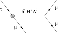
The diagram in Fig. 2 is straightforward to calculate. We derive a branching fraction for $\tau\to 3\mu$ of

$$\mbox{Br}(\tau\to 3\mu)=\frac{G_{F}^{2}m_{\mu}^{2}m_{\tau}^{7}\tau_{\tau}}{768\pi^{3}m_{A}^{4}}\kappa_{32}^{2}\tan^{6}\beta$$ (17)

where $\tau_{\tau}$ is the $\tau$ lifetime. To derive this formula, we took the large $m_{A}$ limit in which $\alpha\to\beta-\pi/2$.

How large can this branching fraction be? Consider the case in which $\mu=M_{1}=M_{2}=m_{{\tilde{\ell}}}=m_{{\tilde{\nu}}}$, $M_{R}=10^{14}\,{\rm GeV}$ and $(Y_{\nu}^{\dagger}Y_{\nu})_{32}=1$. Then $\epsilon_{2}\simeq 4\times 10^{-4}$ and

$$\mbox{Br}(\tau\to 3\mu)\simeq(1\times 10^{-7})\times\left(\frac{\tan\beta}{60}\right)^{6}\times\left(\frac{100\,{\rm GeV}}{m_{A}}\right)^{4}$$ (18)

which puts it into the regime that is experimentally accessible at B-factories over the next few years. At LHC and SuperKEKB, limits in the region of $10^{-9}$ should be achievable [14], allowing a deeper probe into the parameter space. We can also do better if $\mu\gg M_{1,2}\simeq m^{2}_{{\tilde{\ell}}}$. Then the bino contribution is enhanced by a factor $\mu/M_{1}$; for $M_{1}\simeq 100\,{\rm GeV}$ and $\mu\simeq 1\,{\rm TeV}$, one can get $\epsilon_{2}\simeq 8\times 10^{-4}$, resulting in a branching fraction 4 times that stated above. However we note that the value of $\epsilon_{2}\simeq 4\times 10^{-4}$ is remarkably stable to changes in the SUSY spectrum apart from this large-$\mu$ option.

Discussion. We have demonstrated that LFV in the sleptons can generate large LFV in the couplings of leptons to neutral Higgs bosons. It is already well-known that sleptonic flavor violation can induce LFV in certain magnetic moment transitions such as $\tau\to\mu\gamma$, so it is useful to compare this to the $\tau\to 3\mu$ decay which we just found. We first note that the two decays possess very different decoupling behavior so that either one could be large while the other is too small to observe. The effective operator for $\tau\to 3\mu$ is dimension-6: $(1/m_{A}^{2})\overline{\tau}\mu\overline{\mu}\mu$ The $\tau\to\mu\gamma$ operator is formally dimension-5, but chiral symmetry requires an $m_{\tau}$ insertion, so that the operator is actually dimension-6: $(m_{\tau}/M_{\rm SUSY}^{2})\overline{\tau}\sigma^{\mu\nu}\mu F_{\mu\nu}$ where $M_{\rm SUSY}$ represents the heaviest mass scale to enter the slepton-gaugino loops. If sleptons and gauginos are light and $A^{0}$ is heavy, then $\tau\to\mu\gamma$ would tend to dominate; in the opposite limit and with $\tan\beta$ large, $\tau\to 3\mu$ would dominate. Because of this different decoupling behavior, it is impossible to correlate the two decays without choosing a specific model. Turning this around, observation of one or both of these decays can provide insight into the fundamental SUSY-breaking parameters.

The presence of the $\tau\to\mu\gamma$ operator can also lead to $\tau\to 3\mu$ if the photon goes off-shell. However, for this operator the relation between the two branching fractions is roughly model-independent [6]:

$$\frac{\mbox{Br}(\tau\to 3\mu)}{\mbox{Br}(\tau\to\mu\gamma)}\simeq 0.003\quad\mbox{(no Higgs-mediation)}.$$ (19)

If a ratio much larger than $0.003$ is discovered, then this would be clear evidence that some new process is generating the $\tau\to 3\mu$ decay, with Higgs-mediation a leading contender.

Our calculation so far has also relied on Yukawa matrix ansätze which reproduce the mass matrix of Eq. (6). But what if we had made a different choice for $Y_{\nu}^{\dagger}Y_{\nu}$? Another popular option would be the inverted mass hierarchy in which the (1,2) and (1,3) elements of $Y_{\nu}^{\dagger}Y_{\nu}$ would be $O(1)$ and the remainder $O(\epsilon)$ [8]. Such a matrix could lead to observable $\tau\to e\mu\mu$. The constraints coming from $\mu\to e\gamma$ are already strong; for $M_{\rm SUSY}\simeq 100\,{\rm GeV}$ one finds that $(Y_{\nu}^{\dagger}Y_{\nu})_{21}$ has to be $\lower 3.01385pt\hbox{$\;\stackrel{{\scriptstyle\textstyle<}}{{\sim}}\;$}10^{-2}$ [15]. But in the large $M_{\rm SUSY}$, large $\tan\beta$ limit, this bound is weakened and $\tau\to e\mu\mu$ could dominate.

There is another interesting test of the inverted hierarchy models presented by Higgs mediation. The decay $\mu\to 3e$ can also proceed by neutral Higgs exchange. Though the electron Yukawa coupling is tiny, this is offset by the extreme precision of rare $\mu$-decay searches. In particular, we find that for $(Y_{\nu}^{\dagger}Y_{\nu})_{21}=1$,

$$\mbox{Br}(\mu\to 3e)\simeq(5\times 10^{-14})\times\left(\frac{\tan\beta}{60}\right)^{6}\times\left(\frac{100\,{\rm GeV}}{m_{A}}\right)^{4}.$$ (20)

Again, this process can generated by the similar $\mu\to e\gamma$ operator taken off-shell, but there the ratio is again model-independent:

$$\frac{\mbox{Br}(\mu\to 3e)}{\mbox{Br}(\mu\to e\gamma)}\simeq 0.006\quad\mbox{(no Higgs-mediation)}.$$ (21)

Any deviation from this fixed ratio would, as for the taus, be a strong indication of new physics such as that found here.

Finally, we mention here that one could also calculate the rate for processes involving LFV Higgs couplings at both vertices, though we will leave this computation to a future work. For example, a second way to generate $\tau\to e\mu\mu$ would be to use the $\overline{\tau}_{R}\,\mu_{L}$–Higgs coupling that we have been considering in this paper, along with a $\overline{\mu}_{R}e_{L}$–Higgs coupling. We can also generate $\tau\to ee\mu$ with a $\overline{\tau}_{R}\,e_{L}$–Higgs coupling at one end and a $\overline{\mu}_{R}e_{L}$–Higgs coupling at the other. But as above, both processes are constrained by non-observation of $\mu\to e\gamma$ since they require large $(\Delta m^{2}_{{\tilde{L}}})_{21}$. It is notable that these processes have a remarkable $\tan^{8}\beta$ dependence; however the additional powers are mitigated by additional loop suppressions.

Acknowledgments. We would like to thank the scientific staffs of CERN and DESY for their hospitality while this work was completed, and especially P. Zerwas for organizing a thought-provoking SUSY’02 Conference. CK would also like to thank D. Chung and L. Everett for hosting him at their Physics Institute-on-Wheels where much of this letter was composed. This research was supported by the National Science Foundation under grant PHY00-98791, by the U.S. Department of Energy under grants DE-FG03-98ER41076 and DE-FG02-01ER45684, and by a grant from the Research Corporation.

References

- [1] S. Fukuda et al., (SuperKamiokande Collaboration), Phys. Rev. Lett. 85, 3999 (2000).
- [2] S. Fukuda et al., (SuperKamiokande Collaboration), Phys. Rev. Lett. 86, 5656 (2001); Q.R. Ahmad et al., (SNO Collaboration), Phys. Rev. Lett. 87, 071301 (2001) and Phys. Rev. Lett. 89, 011301 (2002).
- [3] M. Gell-Mann, P. Ramond and R. Slansky, in Supergravity, eds. P. van Nieuwenhuizen and D.Z. Freedman (North Holland 1979); T. Yanagida, in Proceedings of the Workshop on Unified Theory and Baryon Number in the Universe, eds. O. Sawada and A. Sugamoto (KEK 1979); R.N. Mohapatra and G. Senjanović, Phys. Rev. Lett. 44, 912 (1980).
- [4] For a review, see: M. C. Gonzalez-Garcia and Y. Nir, arXiv:hep-ph/0202058.
- [5] F. Borzumati and A. Masiero, Phys. Rev. Lett. 57, 961 (1986); L. J. Hall, V. A. Kostelecky and S. Raby, Nucl. Phys. B 267, 415 (1986).
- [6] J. Hisano, T. Moroi, K. Tobe, M. Yamaguchi and T. Yanagida, Phys. Lett. B 357, 579 (1995); J. Hisano, T. Moroi, K. Tobe and M. Yamaguchi, Phys. Rev. D 53, 2442 (1996).
- [7] S. F. King and M. Oliveira, Phys. Rev. D 60, 035003 (1999); J. Hisano and D. Nomura, Phys. Rev. D 59, 116005 (1999); W. Buchmuller, D. Delepine and F. Vissani, Phys. Lett. B 459, 171 (1999); K. S. Babu, B. Dutta and R. N. Mohapatra, Phys. Lett. B 458, 93 (1999); J. R. Ellis et al., Eur. Phys. J. C 14, 319 (2000); J. Sato, K. Tobe and T. Yanagida, Phys. Lett. B 498, 189 (2001); S. Lavignac, I. Masina and C. A. Savoy, Phys. Lett. B 520, 269 (2001); J. A. Casas and A. Ibarra, Nucl. Phys. B 618, 171 (2001).
- [8] For reviews, see: G. Altarelli and F. Feruglio, Phys. Rept. 320, 295 (1999); S. M. Barr and I. Dorsner, Nucl. Phys. B 585, 79 (2000).
- [9] C. H. Albright, K. S. Babu and S. M. Barr, Phys. Rev. Lett. 81, 1167 (1998); J. Sato and T. Yanagida, Phys. Lett. B 430, 127 (1998); N. Irges, S. Lavignac and P. Ramond, Phys. Rev. D 58, 035003 (1998).
- [10] L. J. Hall, R. Rattazzi and U. Sarid, Phys. Rev. D 50, 7048 (1994).
- [11] K. S. Babu and C. Kolda, Phys. Rev. Lett. 84, 228 (2000).
- [12] C. S. Huang, W. Liao, Q. S. Yan and S. H. Zhu, Phys. Rev. D 63, 114021 (2001); A. Dedes, H. K. Dreiner and U. Nierste, Phys. Rev. Lett. 87, 251804 (2001); G. Isidori and A. Retico, JHEP 0111, 001 (2001); R. Arnowitt, B. Dutta, T. Kamon and M. Tanaka, Phys. Lett. B 538, 121 (2002); C. Bobeth et al., arXiv:hep-ph/0204225; H. Baer et al., arXiv:hep-ph/0205325; C. Kolda and J. Lennon, in preparation.
- [13] K. S. Babu, C. Kolda, J. March-Russell and F. Wilczek, Phys. Rev. D 59, 016004 (1999).
- [14] F. Deppisch et al., arXiv:hep-ph/0206122 and references therein.
- [15] Y. G. Kim, P. Ko, J. S. Lee and K. Y. Lee, Phys. Rev. D 59, 055018 (1999); J. Ellis, J. Hisano, M. Raidal and Y. Shimizu, arXiv:hep-ph/0206110.