Abstract

We study the handbag contribution to two-photon annihilation into baryon-antiba-ryon pairs at large energy and momentum transfer. We derive factorization of the process amplitude into a hard $\gamma\gamma\to q\overline{q}$ subprocess and form factors describing the soft $q\overline{q}\to B\overline{B}$ transition, assuming that the process is dominated by configurations where the (anti)quark approximately carries the full momentum of the (anti)baryon. The form factors represent moments of time-like generalized parton distributions, so-called $B\overline{B}$ distribution amplitudes. A characteristic feature of the handbag mechanism is the absence of isospin-two components in the final state, which in combination with flavor symmetry provides relations among the form factors for the members of the lowest-lying baryon octet. Assuming dominance of the handbag contribution, we can describe current experimental data with form factors of plausible size, and predict the cross sections of presently unmeasured $B\overline{B}$ channels.

1 Introduction

In this article we study the annihilation of two photons into baryon-antibaryon ($B\overline{B}$) pairs at large Mandelstam variables $s\sim-t\sim-u$ in the handbag approach recently developed for two-photon annihilation into pairs of mesons [1]. As in the meson case, the handbag amplitude (see Fig. 1) factorizes into a hard $\gamma\gamma\to q\overline{q}$ subprocess and form factors representing moments of generalized distribution amplitudes [2, 3]. These distribution amplitudes are time-like versions of generalized parton distributions, which encode the soft physics information in processes such as deeply virtual [4, 5] or wide-angle [6, 7] Compton scattering. The latter is in fact related to two-photon annihilation by crossing. It is important to realize that, since we take the $B\overline{B}$ system to have large invariant mass, the $q\overline{q}\to B\overline{B}$ transition can only be soft if the additional $q\overline{q}$ and possibly gluon pairs created in the hadronization process have soft momenta. In other words, the initial quark and antiquark must each take approximately the full momentum of one final state hadron. Compared to the case of mesons, our derivation for baryons will make the additional, plausible, assumption that the process is dominated by configurations where it is the quark that approximately moves in the direction of the baryon, whereas the antiquark approximately moves in the direction of the antibaryon. This assumption is equivalent to the valence quark approximation, widely used in other contexts.

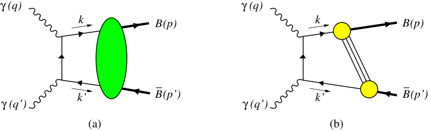
Figure 1: (a) Handbag factorization of baryon pair production $\gamma\gamma\to B\overline{B}$ at large $s$, $t$, and $u$. The hard scattering subprocess is shown at leading order in $\alpha_{s}$, and the blob represents the $B\overline{B}$ distribution amplitude. A second graph is obtained by interchanging the photon vertices. (b) The physical mechanism of the handbag diagrams. The quark hadronizes into $B$ and the antiquark into $\overline{B}$, with any number of soft partons connecting the two parton-hadron vertices.

For both processes, wide-angle Compton scattering off baryons and two-photon annihilation into $B\overline{B}$ pairs, the handbag contribution can dominate for large but not asymptotically large Mandelstam variables. Asymptotically the leading-twist contribution will take over, where in contrast to the handbag mechanism all valence quarks of the involved hadrons participate in the hard scattering [8]. The handbag contribution formally represents a power correction to the leading-twist one. The onset of the leading-twist regime is however expected to occur for $s$ much larger than experimentally available. A more detailed discussion of the relation between the leading-twist and soft handbag mechanisms, and of other power suppressed contributions is given in [1].

Two-photon annihilation into hadrons pairs has also been studied for the case where one of the photons has a virtuality $Q^{2}$ much larger than the squared invariant mass $s$ of the hadron pair. In this kinematics, which is complementary to the one studied in the present article, handbag factorization of the process amplitude has been shown to hold for asymptotically large photon virtualities [2, 3, 9]. In other words, the handbag provides the leading-twist contribution in the limit of large $Q^{2}$ at fixed $s$.

Our paper is organized as follows: In Sect. 2 we define the $B\overline{B}$ distribution amplitudes and discuss some of their properties. Sect. 3 is devoted to the calculation of the handbag amplitude for $\gamma\gamma\to B\overline{B}$. Flavor symmetry properties of the handbag amplitude are investigated in Sect. 4, and a comparison to experiment is presented in Sect. 5. We end our paper with a few concluding remarks.

2 Distribution amplitudes for baryon-antibaryon pairs

Generalized distribution amplitudes for meson pairs have been discussed in detail in the literature [3, 10]. Here we introduce their counterparts for baryon-antibaryon pairs and present some of their general properties. We use light-cone coordinates $v=[v^{+},v^{-},{\bf v}_{\perp}]$ with $v^{\pm}=(v^{0}\pm v^{3})/\sqrt{2}$ for any four-vector $v$, and define $B\overline{B}$ distribution amplitudes in light-cone gauge by

$$P^{+}\int\frac{dx^{-}}{2\pi}\,e^{-izP^{+}x^{-}}\,{}_{\rm out}\big{\langle}\,B(p\nu)\overline{B}(p^{\prime}\nu^{\prime})\,\big{|}\,\overline{q}(\bar{x})\gamma^{+}q(0)\,\big{|}\,0\,\big{\rangle}=$$

$$\qquad\Phi^{q}_{V}(z,\zeta,s)\,\overline{u}(p\nu)\gamma^{+}\,v(p^{\prime}\nu^{\prime})+\Phi^{q}_{S}(z,\zeta,s)\,\frac{P^{+}}{2m}\,\overline{u}(p\nu)\,v(p^{\prime}\nu^{\prime})\,,$$

$$P^{+}\int\frac{dx^{-}}{2\pi}\,e^{-izP^{+}x^{-}}\,{}_{\rm out}\big{\langle}\,B(p\nu)\overline{B}(p^{\prime}\nu^{\prime})\,\big{|}\,\overline{q}(\bar{x})\gamma^{+}\gamma_{5}\,q(0)\,\big{|}\,0\,\big{\rangle}=$$ (1)

$$\qquad\Phi^{q}_{A}(z,\zeta,s)\,\overline{u}(p\nu)\gamma^{+}\gamma_{5}\,v(p^{\prime}\nu^{\prime})+\Phi^{q}_{P}(z,\zeta,s)\,\frac{P^{+}}{2m}\,\overline{u}(p\nu)\gamma_{5}\,v(p^{\prime}\nu^{\prime})$$

with $\bar{x}=[0,x^{-},{\bf 0}_{\perp}]$. Here $m$ denotes the mass of the baryons and $\nu$, $\nu^{\prime}$ their helicities. We have further introduced the sum $P=p+p^{\prime}$ of the baryon momenta, the invariant mass $s=P^{2}$ of the baryon pair, and the skewness

$$\zeta=p^{+}/P^{+}.$$ (2)

In the following we will also use the notation $\overline{\zeta}=1-\zeta$. We have not displayed the dependence of the $B\overline{B}$ distribution amplitudes on the factorization scale $\mu^{2}$, which is governed by the well-known evolution equations for the distribution amplitudes of a single meson with appropriate quantum numbers.

The $B\overline{B}$ distribution amplitudes are the time-like versions of generalized parton distributions for a baryon $B$. Let us briefly comment on the relation of our definitions (1) with those of the generalized parton distributions $H$, $E$, $\tilde{H}$, $\widetilde{E}$, introduced in [4]. Comparing the Lorentz structures that multiply the distributions and taking into account that $p^{\prime+}$ turns into $-p^{\prime+}$ under crossing of $\overline{B}(p^{\prime}\nu^{\prime})$ to $B(p^{\prime}\nu^{\prime})$, we recognize $\Phi_{A}$ and $\Phi_{P}$ as the respective counterparts of $\tilde{H}$ and $\widetilde{E}$. In the vector channel one may use the Gordon decomposition

$$\overline{u}(p\nu)\frac{i}{2m}\,\sigma^{+\rho}(p+\varepsilon\,p^{\prime})_{\rho}\,v(p^{\prime}\nu^{\prime})=\frac{1}{2}(1+\varepsilon)\,\overline{u}(p\nu)\gamma^{+}\,v(p^{\prime}\nu^{\prime})-\frac{1}{2m}\,(p-\varepsilon\,p^{\prime})^{+}\,\overline{u}(p\nu)v(p^{\prime}\nu^{\prime})$$ (3)

with $\varepsilon=\pm 1$ to trade the scalar current for the tensor one. By crossing the defining relation for $H$ and $E$ one would obtain the scalar current $\overline{u}(p\nu)\,v(p^{\prime}\nu^{\prime})$ multiplied with $(p^{\prime}-p)^{+}=(1-2\zeta)P^{+}$ instead of $P^{+}$. Defining a distribution amplitude $\widetilde{\Phi}_{S}$ with such a prefactor would however introduce an artificial singularity of $\widetilde{\Phi}_{S}(z,\zeta,s)$ at $\zeta=\frac{1}{2}$, since there is no symmetry by which $(p^{\prime}-p)^{+}\,\widetilde{\Phi}_{S}(z,\zeta,s)=P^{+}\,\Phi_{S}(z,\zeta,s)$ has to vanish at $p^{+}=p^{\prime+}$. This is in contrast to the case of the generalized parton distribution $\widetilde{E}$, where due to time reversal invariance the product $(p^{\prime}-p)^{+}\widetilde{E}$ occurring in its definition is zero for $p^{+}=p^{\prime+}$.

Integrating (1) over $z$ reduces the bilocal $B\overline{B}$ matrix elements to local ones. In analogy to the space-like case we obtain a set of sum rules,

$$F^{q}_{i}(s) = \int_{0}^{1}dz\;\Phi^{q}_{i}\,(z,\zeta,s)\qquad\mbox{for~{}}i=V,A,P\,,$$

$$(1-2\zeta)\,F^{q}_{S}(s) = \int_{0}^{1}dz\;\Phi^{q}_{S}\,(z,\zeta,s)$$ (4)

with time-like form factors defined as

$${}_{\rm out}\big{\langle}\,B(p\nu)\overline{B}(p^{\prime}\nu^{\prime})\,\big{|}\,\overline{q}(0)\gamma^{\rho}q(0)\,\big{|}\,0\,\big{\rangle} = F^{q}_{V}\,\overline{u}(p\nu)\gamma^{\rho}\,v(p^{\prime}\nu^{\prime})+F^{q}_{S}\,\frac{(p^{\prime}-p)^{\rho}}{2m}\,\overline{u}(p\nu)\,v(p^{\prime}\nu^{\prime})\,,$$ (5)

$${}_{\rm out}\big{\langle}\,B(p\nu)\overline{B}(p^{\prime}\nu^{\prime})\,\big{|}\,\overline{q}(0)\gamma^{\rho}\gamma_{5}\,q(0)\,\big{|}\,0\,\big{\rangle} = F^{q}_{A}\,\overline{u}(p\nu)\gamma^{\rho}\gamma_{5}\,v(p^{\prime}\nu^{\prime})+F^{q}_{P}\,\frac{(p^{\prime}+p)^{\rho}}{2m}\,\overline{u}(p\nu)\gamma_{5}\,v(p^{\prime}\nu^{\prime})$$

for each flavor. Appropriate combinations give the form factors of the electromagnetic and weak currents, for instance the magnetic and Pauli form factors

$$G_{M}(s)=\sum_{q}\,e_{q}\,F^{q}_{V}(s),\qquad F_{2}(s)=\sum_{q}\,e_{q}\,F^{q}_{S}(s).$$ (6)

The relations (4) are valid for any physical value of the skewness $\zeta$. They also hold for any value of the factorization scale $\mu^{2}$ of the distribution amplitudes, since the vector and axial vector currents have zero anomalous dimension and the form factors $F_{V,S}$ and $F_{A,P}$ are scale independent. Taking higher moments in $(2z-1)$ leads to $\mu^{2}$ dependent form factors of local operators with derivatives, multiplied by polynomials in $(2\zeta-1)$.

From charge-conjugation invariance we find the symmetry relations

$$\Phi^{q}_{i}(z,\zeta,s) = \hskip 12.91663pt\Phi^{q}_{i}(\overline{z},\overline{\zeta},s)\qquad\mbox{for~{}}i=V,A,P\,,$$

$$\Phi^{q}_{S}(z,\zeta,s) = {}-\Phi^{q}_{S}(\overline{z},\overline{\zeta},s)$$ (7)

with $\overline{z}=1-z$. For $\zeta=\frac{1}{2}$ the distribution amplitudes $\Phi_{V,A,P}$ are hence symmetric under the replacement $z\leftrightarrow\overline{z}$, while $\Phi_{S}$ is antisymmetric (but not zero). One may consider $B\overline{B}$-states of definite charge-conjugation symmetry

$${\big{|}}\,{C\pm}{\big{\rangle}}=\frac{1}{2}\,{\Big{|}}B(p,\nu)\,\overline{B}(p^{\prime}\nu^{\prime})\,\,\mp\,B(p^{\prime},\nu^{\prime})\,\overline{B}(p\nu)\Big{\rangle}\,,$$ (8)

satisfying

$${\cal C}\,\big{|}\,{C\pm}\,\big{\rangle}=\pm\,\big{|}\,{C\pm}\,\big{\rangle}\,,$$ (9)

where the operator ${\cal C}$ implements charge conjugation in Hilbert space. Replacing the state $\langle\,B(p,\nu)\,\overline{B}(p^{\prime}\nu^{\prime})\,|$ with $\langle\,{C\pm}|$ in the definition (1), we obtain on its right-hand side the linear combinations

$$\Phi^{q(\pm)}_{i}(z,\zeta,s) = \frac{1}{2}\Big{[}\Phi^{q}_{i}(z,\zeta,s)\mp\Phi^{q}_{i}(\overline{z},{\zeta},s)\Big{]}\qquad\mbox{~{}for~{}}i=V,S\,,$$ (10)

$$\Phi^{q(\pm)}_{i}(z,\zeta,s) = \frac{1}{2}\Big{[}\Phi^{q}_{i}(z,\zeta,s)\pm\Phi^{q}_{i}(\overline{z},{\zeta},s)\Big{]}\qquad\mbox{~{}for~{}}i=A,P\,,$$ (11)

where we have used the symmetry relations (7). With the same relations one finds that $\Phi_{V}^{q(+)}$ and $\smash{\Phi_{S,A,P}^{q(-)}}$ are odd under the replacement $\zeta\leftrightarrow\overline{\zeta}$, which implies zeroes of these distribution amplitudes at $\zeta=\frac{1}{2}$. Note also that the $C$-even combinations $\Phi_{V,S}^{q(+)}$ are antisymmetric under the replacement $z\leftrightarrow\overline{z}$ and therefore disappear in the sum rules (4). This is consistent with the properties of the form factors $F_{V}$ and $F_{S}$, which are $C$-odd. The reverse situation occurs for the $C$-odd combinations $\Phi_{A,P}^{q(-)}$, which do not enter (4) in agreement with the $C$-even nature of $F_{A}$ and $F_{P}$.

The distribution amplitudes $\Phi_{i}(z,\zeta,s)$ are complex quantities, with phases due to the interactions in the $B\overline{B}$ system. Because of time reversal invariance they also parameterize matrix elements with baryons in the initial state,

$$P^{+}\int\frac{dx^{-}}{2\pi}\,e^{izP^{+}x^{-}}\,\big{\langle}0\,\big{|}\,\overline{q}(0)\gamma^{+}q(\bar{x})\,\big{|}\,B(p\nu)\overline{B}(p^{\prime}\nu^{\prime})\,\big{\rangle}_{\rm in}=$$

$$\qquad\Phi^{q}_{V}(z,\zeta,s)\,\overline{v}(p^{\prime}\nu^{\prime})\gamma^{+}\,u(p\nu)+\Phi^{q}_{S}(z,\zeta,s)\,\frac{P^{+}}{2m}\,\overline{v}(p^{\prime}\nu^{\prime})\,u(p\nu)\,,$$

$$P^{+}\int\frac{dx^{-}}{2\pi}\,e^{izP^{+}x^{-}}\,\big{\langle}0\,\big{|}\,\overline{q}(0)\gamma^{+}\gamma_{5}\,q(\bar{x})\,\big{|}\,B(p\nu)\overline{B}(p^{\prime}\nu^{\prime})\,\big{\rangle}_{\rm in}=$$ (12)

$$\qquad\Phi^{q}_{A}(z,\zeta,s)\,\overline{v}(p^{\prime}\nu^{\prime})\gamma^{+}\gamma_{5}\,u(p\nu)-\Phi^{q}_{P}(z,\zeta,s)\,\frac{P^{+}}{2m}\,\overline{v}(p^{\prime}\nu^{\prime})\gamma_{5}\,u(p\nu).$$

Notice the change of sign in front of $\Phi_{P}$.

We finally remark that distribution amplitudes for pairs $B_{1}\overline{B}_{2}$ involving different baryons can be defined as in (1). The charge conjugation relations (7) do not hold for these quantities, but they do for distribution amplitudes of the symmetrized states $|B_{1}(p\nu)\,\overline{B}_{2}(p^{\prime}\nu^{\prime})+B_{2}(p\nu)\,\overline{B}_{1}(p^{\prime}\nu^{\prime})\rangle$.

3 The handbag amplitude

We will now derive the expression for the soft handbag contribution to $\gamma\gamma\to B\overline{B}$. The first steps of the derivation go in complete analogy to the case of meson pair production. We thus start by summarizing the corresponding results of [1], and then proceed from the point where the different nature of baryons and mesons leads to important differences. In [1] we found an appropriate frame to be the c.m. of the reaction, with axes chosen such that the process takes place in the 1-3 plane and the outgoing hadrons fly along the positive or negative 1-direction. Thus, we have baryon momenta

$$p=\sqrt{\frac{s}{8}}\left[\,1\,,\,1\,,\,\sqrt{2}\beta\,{\bf e}_{1}\,\right],\qquad p^{\prime}=\sqrt{\frac{s}{8}}\left[\,1\,,\,1\,,\,-\sqrt{2}\beta\,{\bf e}_{1}\,\right],$$ (13)

with the relativistic velocity $\beta=\sqrt{1-4m^{2}/s}$ and ${\bf e}_{1}=(1,0)$. We hence have skewness $\zeta=\frac{1}{2}$. The photon momenta read

$$q = \sqrt{\frac{s}{8}}\left[\,1+\sin\theta\,,\,1-\sin\theta\,,\,\sqrt{2}\cos\theta\,{\bf e}_{1}\,\right],$$

$$q^{\prime} = \sqrt{\frac{s}{8}}\left[\,1-\sin\theta\,,\,1+\sin\theta\,,\,-\sqrt{2}\cos\theta\,{\bf e}_{1}\,\right],$$ (14)

where $\theta$ is the c.m. scattering angle. In terms of the usual Mandelstam variables we have

$$\cos\theta=\frac{t-u}{s},\qquad\sin\theta=\frac{2\sqrt{t\,u}}{s}$$ (15)

up to corrections of order $m^{2}/s$. The handbag amplitude for our process can be written in terms of the hard scattering kernel for $\gamma\gamma\to q\overline{q}$

$$H_{\alpha\beta}(k,k^{\prime})=\left[\epsilon\cdot\gamma\,\frac{(k-q)\cdot\gamma}{(k-q)^{2}+i\epsilon}\,\epsilon^{\prime}\cdot\gamma+\epsilon^{\prime}\cdot\gamma\,\frac{(q-k^{\prime})\cdot\gamma}{(q-k^{\prime})^{2}+i\epsilon}\,\epsilon\cdot\gamma\right]_{\alpha\beta}$$ (16)

with photon polarization vectors $\epsilon=\epsilon(q,\mu)$ and $\epsilon^{\prime}=\epsilon(q^{\prime},\mu^{\prime})$, and a matrix element describing the $q\overline{q}\to B\overline{B}$ transition. Our starting expression thus is

$${\cal A}=\sum_{q}(ee_{q})^{2}\int\!d^{4}k\,\int\!\frac{d^{4}x}{(2\pi)^{4}}\,e^{-ik\cdot x}\,{}_{\rm out}\big{\langle}B(p\nu)\,\overline{B}(p^{\prime}\nu^{\prime})\,\big{|}\,T\,\overline{q}{}_{\alpha}(x)\,q_{\beta}(0)\,\big{|}0\big{\rangle}\;H_{\alpha\beta}(k,k^{\prime})\,,$$ (17)

where the summation index $q$ refers to the quark flavors $u$, $d$, $s$. In $H$ we have omitted terms suppressed by the current quark masses.

As discussed in detail in [1], the $q\overline{q}\to B\overline{B}$ transition at large invariant mass $s$ can only be soft if the incoming quark and antiquark have small virtualities and each carry approximately the momentum of the baryon or antibaryon. To quantify this, we define $z=k^{+}/P^{+}$ and parameterize the on-shell approximations of the quark and antiquark momenta $k$ and $k^{\prime}$ as

$$\tilde{k}=\sqrt{\frac{s}{2}}\left[\,z,\,\bar{z},\,\sqrt{2z\bar{z}}\,{\bf e}_{\perp}\,\right],\qquad\tilde{k}^{\prime}=\sqrt{\frac{s}{2}}\left[\,\bar{z},\,z,\,-\sqrt{2z\bar{z}}\,{\bf e}_{\perp}\,\right],$$ (18)

where ${\bf e}_{\perp}=(\cos\varphi,\sin\varphi)$. The requirements derived in [1] then read

$$2z-1,\,\sin\varphi\sim\frac{\Lambda^{2}}{s}\,,$$ (19)

where $\Lambda$ is a hadronic scale of order 1 GeV. In addition, the minus- and transverse momenta of $k-\tilde{k}$ and $k^{\prime}-\tilde{k}^{\prime}$ must be of order $\Lambda^{2}/\sqrt{s}$. As shown in [1, 7], the dominant Dirac structure of the soft matrix element in (17) involves the good components of the quark fields in the parlance of light-cone quantization. Projecting these out we have

$${\cal A}_{\nu\nu^{\prime},\mu\mu^{\prime}}=-\sum_{q}(ee_{q})^{2}\int\!d^{4}k\,\frac{1}{\sqrt{4k^{+}k^{\prime+}}}\,\left[\,{\cal H}_{\mu\mu^{\prime}}(\tilde{k},\tilde{k}^{\prime})\,{\cal S}_{q}(k,k^{\prime})+{\cal H}^{5}_{\mu\mu^{\prime}}(\tilde{k},\tilde{k}^{\prime})\,{\cal S}^{5}_{q}(k,k^{\prime})\,\right]+{\cal O}(\Lambda^{2}/s)\,,$$ (20)

where we have now made explicit the dependence on the photon and baryon helicities $\mu$, $\mu^{\prime}$ and $\nu$, $\nu^{\prime}$, respectively. Here we have introduced the soft matrix elements

$${\cal S}_{q}=\frac{1}{2}\int\!\frac{d^{4}x}{(2\pi)^{4}}\,e^{-ik\cdot x}\,{}_{\rm out}\big{\langle}\,B(p\nu)\overline{B}(p^{\prime}\nu^{\prime})\big{|}\,T\,\overline{q}(x)\,\gamma^{+}q(0)\,\big{|}\,0\big{\rangle}\,,$$ (21)

and ${\cal S}^{5}_{q}$ with $\gamma^{+}$ replaced by $\gamma^{+}\gamma_{5}$. The hard subprocess amplitudes of $\gamma\gamma\to q\overline{q}$ for the helicity sum and difference of the quark read

$${\cal H}_{\mu\mu^{\prime}}(\tilde{k},\tilde{k}^{\prime}) = \sum_{\lambda=\pm 1/2}\phantom{\lambda}\overline{u}(\tilde{k},\lambda)\,H_{\mu\mu^{\prime}}(\tilde{k},\tilde{k}^{\prime})\,v(\tilde{k}^{\prime},-\lambda)\,,$$

$${\cal H}^{5}_{\mu\mu^{\prime}}(\tilde{k},\tilde{k}^{\prime}) = \sum_{\lambda=\pm 1/2}2\lambda\;\overline{u}(\tilde{k},\lambda)\,H_{\mu\mu^{\prime}}(\tilde{k},\tilde{k}^{\prime})\,v(\tilde{k}^{\prime},-\lambda)\,,$$ (22)

where we have approximated the parton momenta with their on-shell values. The expressions (20) and (22) imply the phase conventions for light-cone spinors given in the appendix. With these conventions the behavior of helicity amplitudes under a parity transformation is ${\cal A}_{\nu\nu^{\prime},\mu\mu^{\prime}}=\eta\,(-1)^{\nu-\nu^{\prime}-\mu+\mu^{\prime}}{\cal A}_{-\nu-\nu^{\prime},-\mu-\mu^{\prime}}$, where $\eta$ is the product of the intrinsic parities of the four particles involved.

According to our hypothesis that the $q\overline{q}\to B\overline{B}$ transition is dominated by soft processes, the matrix elements ${\cal S}_{q}(k,k^{\prime})$ and ${\cal S}^{5}_{q}(k,k^{\prime})$ should be strongly peaked when (19) is fulfilled. Depending on whether $\varphi\approx 0$ or $\varphi\approx\pi$ this means that we have $k\approx p$ or $k^{\prime}\approx p$. The case $k^{\prime}\approx p$ corresponds to the antiquark hadronizing into $B$ and the quark into $\overline{B}$. This requires sea quarks with very high momentum fraction in a baryon. We expect this to be disfavored compared with the case $k\approx p$, both from phenomenological and theoretical considerations. A rather direct piece of information is for instance the ratio of quark and antiquark distributions in a nucleon at large momentum fraction $x$. Neglecting configurations with $k^{\prime}\approx p$ compared with $k\approx p$, we proceed by Taylor expanding ${\cal H}(\tilde{k},\tilde{k}^{\prime})$ and ${\cal H}^{5}(\tilde{k},\tilde{k}^{\prime})$ around $z=\frac{1}{2}$ and $\varphi=0$, keeping only the leading order in $\Lambda^{2}/s$ . We get ${\cal H}^{(5)}_{--}={\cal H}^{(5)}_{++}=0$ and

$${\cal H}_{+-}(\tilde{k},\tilde{k}^{\prime}) = \phantom{-}{\cal H}_{-+}(\tilde{k},\tilde{k}^{\prime})\>=\>2\,\Big{(}\sqrt{\hat{u}/\hat{t}}-\sqrt{\hat{t}/\hat{u}}\,\Big{)}\>=\>2\,\frac{t-u}{\sqrt{tu}}+{\cal O}(\Lambda^{2}/s),$$

$${\cal H}^{5}_{+-}(\tilde{k},\tilde{k}^{\prime}) = -{\cal H}^{5}_{-+}(\tilde{k},\tilde{k}^{\prime})\>=\>2\,\Big{(}\sqrt{\hat{u}/\hat{t}}+\sqrt{\hat{t}/\hat{u}}\,\Big{)}\>=\>2\,\frac{s}{\sqrt{tu}}+{\cal O}(\Lambda^{2}/s),$$ (23)

where $\hat{t}$ and $\hat{u}$ are the Mandelstam variables of the hard subprocess, with quark and antiquark momenta put on shell. For better legibility, explicit helicities are labeled only by their signs here and in the following. The amplitudes with equal photon helicities $\mu=\mu^{\prime}$ will be nonzero at next-to-leading order in $\alpha_{\rm s}$, in analogy to the photon helicity flip transitions in large-angle Compton scattering [11]. With (23) the loop integration in (20) now only concerns the soft matrix elements and leads to moments of $B\overline{B}$ distribution amplitudes. With $dk^{+}/\sqrt{4k^{+}k^{\prime}{}^{+}}\simeq dz$ and the definitions of Sect. 2 we obtain

$${\cal A}_{\nu\nu^{\prime},\mu\mu^{\prime}} = -\sum_{q}(ee_{q})^{2}\int_{0}^{1}\!dz\,\left\{{\cal H}_{\mu\mu^{\prime}}(p,p^{\prime})\,\Big{[}\Phi_{V}^{q}\,(z,\zeta={\textstyle\frac{1}{2}},s)\,\frac{1}{2P^{+}}\,\overline{u}(p\nu)\gamma^{+}\,v(p^{\prime}\nu^{\prime})\right.$$

$$\hskip 120.00018pt+\,\Phi_{S}^{q}\,(z,\zeta={\textstyle\frac{1}{2}},s)\,\frac{1}{4m}\,\overline{u}(p\nu)\,v(p^{\prime}\nu^{\prime})\,\Big{]}$$

$$\hskip 71.00017pt+\,{\cal H}^{5}_{\mu\mu^{\prime}}(p,p^{\prime})\,\Big{[}\Phi_{A}^{q}\,(z,\zeta={\textstyle\frac{1}{2}},s)\,\frac{1}{2P^{+}}\,\overline{u}(p\nu)\gamma^{+}\gamma_{5}\,v(p^{\prime}\nu^{\prime})$$

$$\hskip 120.00018pt\left.+\,\Phi_{P}^{q}\,(z,\zeta={\textstyle\frac{1}{2}},s)\,\frac{1}{4m}\,\overline{u}(p\nu)\gamma_{5}\,v(p^{\prime}\nu^{\prime})\,\Big{]}\right\}\;+\;{\cal O}(\Lambda^{2}/s)\,.$$

Because of (7) the scalar distribution amplitude $\Phi_{S}$ decouples in our frame with $\zeta={\textstyle\frac{1}{2}}$. Evaluating the spinor products with the conventions given in the appendix, including terms suppressed only by $m/\sqrt{s}$, we arrive at our final result for the $\gamma\gamma\to B\overline{B}$ amplitudes:

$${\cal A}_{\nu\nu^{\prime},+-}=-(-1)^{\nu-\nu^{\prime}}\,{\cal A}_{-\nu-\nu^{\prime},-+}=4\pi\alpha_{\rm elm}\;\frac{s}{\sqrt{tu}}$$

$$\times \left\{\delta_{\nu-\nu^{\prime}}\,\frac{t-u}{s}\,R_{V}(s)\;+\;2\nu\delta_{\nu-\nu^{\prime}}\Big{[}R_{A}(s)+R_{P}(s)\Big{]}\;-\;\frac{\sqrt{s}}{2m}\,\delta_{\nu\nu^{\prime}}\,R_{P}(s)\right\}\;+\;{\cal O}(\Lambda^{2}/s)\,,$$

where we have defined the annihilation form factors by

$$R_{i}(s)=\sum_{q}e_{q}^{2}\,F^{q}_{i}(s)\qquad\mbox{for~{}}i=V,A,P\,,$$ (26)

with $F^{q}_{i}$ from (4). As in wide-angle Compton scattering off baryons [7] there are only three independent form factors. In Compton scattering it is the pseudoscalar rather than the scalar form factor that does not contribute, due to different choices of the reference frames. The unpolarized differential cross section is given by

$$\frac{d\sigma}{dt}(\gamma\gamma\to B\overline{B})=\frac{4\pi\alpha_{\rm elm}^{2}}{s^{2}}\,\frac{1}{\sin^{2}\theta}\;\left\{\,\Big{|}R_{V}(s)\Big{|}^{\,2}\,\cos^{2}\theta\,+\,\Big{|}R_{A}(s)+R_{P}(s)\Big{|}^{\,2}\,+\,\frac{s}{4m^{2}}\,\Big{|}R_{P}(s)\Big{|}^{\,2}\,\right\}\,.$$ (27)

Several comments on our result (3) are in order. Unlike $R_{A}$ and $R_{P}$, the vector form factor $R_{V}$ projects on the $C$ odd part of the $B\overline{B}$ state, whereas a $\gamma\gamma$ collision produces of course its $C$ even projection. This is a result of the approximations that lead from (20) to (3), namely of neglecting configurations where the $\overline{q}$ emerging from the two-photon annihilation hadronizes into the baryon $B$ instead of the antibaryon $\overline{B}$. To take this contribution into account, one can split the loop integration over ${\bf k}_{\perp}=(k^{1},k^{2})$ into the two hemispheres where $k^{1}$ is either positive or negative. In the former case one can expand the hard scattering amplitudes around $\varphi=0$, and in the latter around $\varphi=\pi$. For $\varphi=\pi$ we then get ${\cal H}_{+-}\approx 2(u-t)/\sqrt{tu}$ instead of $2(t-u)/\sqrt{tu}$ as in (23). The sum over both hemispheres thus gives a result proportional to ${\cal H}_{+-}(p,p^{\prime})$ times

$$\int dk^{-}d^{2}{\bf k}_{\perp}\;\mbox{sgn}(k^{1})\,{\cal S}_{q}(k,k^{\prime})\,,$$ (28)

instead of the integral

$$\int dk^{-}d^{2}{\bf k}_{\perp}\;{\cal S}_{q}(k,k^{\prime})\,,$$ (29)

which we used to express our result in terms of the distribution amplitude $\Phi_{V}$. The integrated matrix elements (28) and (29) have opposite behavior under charge conjugation, but to the extent that the region $k\approx p^{\prime}$ gives a small contribution compared to the region $k\approx p$, their difference can be neglected. In our derivation we have preferred the form (29) that leads to matrix elements of light-cone operators with well-known properties, at the price of a loss in accuracy which we do not expect to be critical. We remark that for baryon helicities $\nu=\nu^{\prime}$ both (28) and (29) are odd under $z\leftrightarrow\overline{z}$ in our reference frame, which results in a zero contribution to the amplitude after integration over $z$. This can be shown by performing a charge conjugation followed by a rotation of $180^{\circ}$ around the $3$-axis. The amplitudes with opposite baryon helicities $\nu=-\nu^{\prime}$ do not decouple in this way, because charge conjugation exchanges the helicities of $B$ and $\overline{B}$. We finally emphasize that the amplitude (3) for the $\gamma\gamma\to B\overline{B}$ process does have the correct behavior under charge conjugation, which for our spinor convention reads ${\cal A}_{\nu\nu^{\prime},\mu\mu^{\prime}}=(-1)^{\nu-\nu^{\prime}-\mu+\mu^{\prime}}{\cal A}_{\nu^{\prime}\nu,\mu^{\prime}\mu}$ in this channel.

For the sake of comparison let us mention what happens if we make the corresponding approximations in wide-angle Compton scattering. Using that contributions where a fast antiquark is emitted from and reabsorbed by the baryon are small, one may count them with the “wrong” sign in the Compton form factors $R_{V}(t)$ and $R_{T}(t)$ of [7]. Replacing then the explicit factors $1/x$ with $1$, we obtain approximations $R_{V}(t)\approx\sum_{q}^{\phantom{2}}e_{q}^{2}\,F_{1}^{q}(t)$ and $R_{T}(t)\approx\sum_{q}^{\phantom{2}}e_{q}^{2}\,F_{2}^{q}(t)$ in terms of the space-like Dirac and Pauli form factors, in analogy with our result here.

The amplitude (3) shows important differences compared with the one we obtained in [1] for production of a pair of pseudoscalar mesons. Similarly to the $B\overline{B}$ amplitudes with $\nu=\nu^{\prime}$, the matrix element corresponding to (28) vanishes there when integrated over $z$. Due to parity invariance the corresponding contribution from ${\cal S}^{5}_{q}$ is also zero, so that the leading term in the Taylor expansion (23) of the hard subprocess gives a vanishing scattering amplitude. We thus had to include the first nonleading term in this expansion, which is proportional to $z-\overline{z}$. If one were to do the same in the $B\overline{B}$ case, one would get a further term in (3). It would involve $\int dz(2z-1)\,\Phi_{S}(z,\frac{1}{2},s)$, which is a form factor of the quark energy-momentum-tensor, in analogy to the meson pair case. Such a subleading contribution would behave as $1/(tu)$ in the amplitude instead of $1/\sqrt{tu}$, and give a $1/\sin^{4}\theta$ rather than $1/\sin^{2}\theta$ dependence in the cross section.

Returning to our result (3), we observe that the pseudoscalar annihilation form factor $R_{P}$ generates amplitudes with equal helicities of the baryon and antibaryon, i.e., with their spin projections along ${\bf p}$ coupled to zero. The spins of quark and antiquark in the $q\overline{q}\to B\overline{B}$ transition do then not sum up to those of the $B\overline{B}$ system, which implies that parton configurations with non-zero orbital angular momentum along ${\bf p}$ are required in $R_{P}$. One expects that at large $s$ such quantities are suppressed compared with $R_{V}$ or $R_{A}$. An analog in the space-like region are the form factors $R_{T}(t)$ vs. $R_{V}(t)$, and their electromagnetic counterparts $F_{2}(t)$ vs. $F_{1}(t)$. Recent measurements from Jefferson Lab [12] indicate that for $-t$ between 1 and 5.6 GeV² the ratio $F_{2}(t)/F_{1}(t)$ approximately scales as $m/\sqrt{-t}$. Assuming a similar behavior of $R_{P}(s)/R_{A}(s)$ one finds that the term with $s|R_{P}(s)|^{2}$ in (27) will not start do dominate over the other terms with increasing $s$.

We see in (27) that the form factor $R_{V}$ can be separated from the two others through measurement of the angular distribution of the $B\overline{B}$ pair, given data of sufficient accuracy. This requires some lever arm in $\theta$, but must stay within the validity of our approach, which is not applicable for $\theta$ near $0$ or $\pi$, where the $\gamma\gamma\to q\overline{q}$ subprocess is no longer hard.

A separation of $R_{A}$ and $R_{P}$ can only be performed with suitable polarization measurements. Our amplitudes (3) are evaluated for states with definite light-cone helicities, which is natural within our framework and leads to simple expressions. In the unpolarized cross section this does not matter, but for polarization observables the use of the ordinary c.m.s. helicity basis is more convenient. The transformation from one helicity basis to the other can be found in [13]. In our kinematics, the c.m.s. helicity amplitudes ${\cal M}$ read

$${\cal M}_{\nu\nu^{\prime},\mu\mu^{\prime}}\,=\,{\cal A}_{\nu\nu^{\prime},\mu\mu^{\prime}}\,+\frac{m}{\sqrt{s}}\,\left[\,2\nu{\cal A}_{-\nu\nu^{\prime},\mu\mu^{\prime}}\,+\,2\nu^{\prime}{\cal A}_{\nu-\nu^{\prime},\mu\mu^{\prime}}\,\right]\,+\,{\cal O}(m^{2}/s)\,.$$ (30)

An observable capable of separating $R_{P}$ from the other form factors is, for instance, the helicity correlation $C_{LL}$ between baryon and antibaryon, given by

$$C_{LL}=\frac{d\sigma{(++)}-d\sigma{(+-)}}{d\sigma{(++)}+d\sigma{(+-)}}=-\,\frac{\Big{|}R_{A}(s)+R_{P}(s)\Big{|}^{\,2}+\cos^{2}\theta\Big{|}R_{V}(s)\Big{|}^{\,2}-\frac{s}{4m^{2}}\Big{|}R_{P}(s)\Big{|}^{\,2}}{\Big{|}R_{A}(s)+R_{P}(s)\Big{|}^{\,2}+\cos^{2}\theta\Big{|}R_{V}(s)\Big{|}^{\,2}+\frac{s}{4m^{2}}\Big{|}R_{P}(s)\Big{|}^{\,2}}\,,$$ (31)

where $d\sigma(\nu,\nu^{\prime})$ is the cross section for polarized $B\overline{B}$ production.

One may also consider the time-reversed process $B\overline{B}\to\gamma\gamma$, which for the case of proton-antiproton collisions may be experimentally accessible and has already been mentioned in [14]. Time reversal invariance relates the amplitudes of both processes by

$${\cal A}_{\mu\mu^{\prime},\,\nu\nu^{\prime}}^{B\overline{B}\to\gamma\gamma}\;(s,t)={\cal A}_{\nu\nu^{\prime},\,\mu\mu^{\prime}}^{\gamma\gamma\to B\overline{B}}\;(s,t)\,.$$ (32)

Up to an extra $(1-4m^{2}/s)^{-1}$ in the phase space factor, $B\overline{B}\to\gamma\gamma$ has therefore the same cross section as $\gamma\gamma\to B\overline{B}$. The relation between the $B\overline{B}$ distribution amplitudes for baryons in the initial or in the final state has already been given in Sect. 2. As in the case of wide-angle Compton scattering [15], one can finally generalize our approach to the case of virtual photons, provided their virtualities are at most of order $s$.

4 Flavor symmetry

We are now going to discuss various $B\overline{B}$ channels where $B$ is a member of the lowest-lying octet of baryons. We shall derive relations among the various amplitudes and form factors in order to simplify the analysis of experimental data on these cross section, and to explore generic consequences of soft handbag dominance.

Relations among the various $B\overline{B}$ channels are obtained by exploiting flavor symmetry, i.e. isospin and $U$-spin invariance. The latter is the symmetry under the exchange $d\leftrightarrow s$, and relates for instance the $p\overline{p}$ and the $\Sigma^{+}\overline{\Sigma}{}^{-}$ channels. Since the photon behaves as a $U$-spin singlet while $(p,\Sigma^{+})$ and $(\overline{\Sigma}{}^{-},\overline{p})$ are doublets, $U$-spin conservation leads to

$$\rule[-5.0pt]{0.0pt}{20.00003pt}{\cal A}(\Sigma^{+}\overline{\Sigma}{}^{-})\,\simeq\,{\cal A}(p\overline{p})\,.$$ (33)

In contrast to isospin breaking, which is known to hold on the percent level and will be neglected here, $U$-spin violations cannot numerically be ignored. This is indicated in (33) and in later relations by the approximate symbol. In analogy to (33) one has

$${\cal A}(\Xi^{-}\overline{\Xi}{}^{+})\,\simeq\,{\cal A}(\Sigma^{-}\overline{\Sigma}{}^{+})\,.$$ (34)

Other consequences of $U$-spin symmetry hold for the $U$-spin triplet $\big{(}n,{\textstyle\frac{1}{2}}[\Sigma^{0}+\sqrt{3}\Lambda],\Xi^{0}\big{)}$ and the $U$-spin singlet ${\textstyle\frac{1}{2}}[\Lambda-\sqrt{3}\Sigma^{0}]$. Together with the corresponding transformation properties of the antiparticles one obtains

$${\cal A}(\Xi^{0}\overline{\Xi}{}^{0}) \simeq {\cal A}(n\overline{n})\hskip 6.00006pt\;\simeq\;\frac{1}{2}\,\Big{[}{\cal A}(\Sigma^{0}\overline{\Sigma}{}^{0})-3{\cal A}(\Lambda\overline{\Lambda})\,\Big{]}\,,$$

$${\cal A}(\Lambda\overline{\Sigma}{}^{0}) \simeq {\cal A}(\Sigma^{0}\overline{\Lambda})\;\simeq\;\frac{\sqrt{3}}{2}\,\Big{[}{\cal A}(\Lambda\overline{\Lambda})-{\cal A}(\Sigma^{0}\overline{\Sigma}{}^{0})\,\Big{]}\,.$$ (35)

Notice that the preceding $U$-spin relations hold in any dynamical approach respecting SU(3) flavor symmetry.

To proceed, we use that the handbag mechanism involves intermediate $q\overline{q}$ states,

$$\gamma\gamma\to q\overline{q}\to B\overline{B}\,,$$ (36)

and generically decompose the $\gamma\gamma$ amplitudes as

$${\cal A}(B\overline{B})=\sum_{q}e^{2}_{q}A_{q}^{B}\,.$$ (37)

We have omitted helicity labels since the following results hold for any set of helicities. The decomposition (37) already follows from (17) and thus is more general than our result (3). It does not rely on our neglect of various ${\cal O}(\Lambda^{2}/s)$ effects, nor of contributions where a fast $\overline{q}$ hadronizes into a baryon.

A characteristic feature of the handbag mechanism is that the intermediate $q\overline{q}$ state can only be coupled to isospin $I=0$ and $I=1$, but not to $I=2$. This leads to particular strong restrictions in the $\Sigma$ sector, where it reduces the number of independent partial amplitudes $A_{q}^{\Sigma}$ to three, one for each flavor. The absence of the isospin-two component of $\Sigma\overline{\Sigma}$ implies the following relation for the amplitudes:

$${\cal A}(\Sigma^{0}\overline{\Sigma}{}^{0})=-\frac{1}{2}\,\Big{[}{\cal A}(\Sigma^{-}\overline{\Sigma}{}^{+})\,+\,{\cal A}(\Sigma^{+}\overline{\Sigma}{}^{-})\,\Big{]}\,,$$ (38)

which provides bounds on the (integrated or differential) $\Sigma^{0}\overline{\Sigma}{}^{0}$ cross section,

$$\frac{1}{2}\,\left|\sqrt{\sigma(\Sigma^{+}\overline{\Sigma}{}^{-})}-\sqrt{\sigma(\Sigma^{-}\overline{\Sigma}{}^{+}})\right|\leq\sqrt{\sigma(\Sigma^{0}\overline{\Sigma}{}^{0})}\leq\frac{1}{2}\,\left(\sqrt{\sigma(\Sigma^{+}\overline{\Sigma}{}^{-})}+\sqrt{\sigma(\Sigma^{-}\overline{\Sigma}{}^{+})}\,\right)\,.$$ (39)

This follows from isospin invariance alone and thus is a robust prediction of handbag dominance.

Combining the relations due to isospin and to $U$-spin, in particular the absence of final states with $I=2$ for the handbag, we find that all $B\overline{B}$ channels are described by only three independent partial amplitudes, which one may take to be those of the $p\overline{p}$ channel, $A^{p}_{u}$, $A^{p}_{d}$ and $A^{p}_{s}$. The compiled relations of the other partial amplitudes to the proton ones read

$$A_{u}^{n} = A_{d}^{p}\,,\hskip 76.82234ptA_{d}^{n}\;=A_{u}^{p}\,,\hskip 79.6678ptA_{s}^{n}\>\>\,=\>A_{s}^{p}\,,\phantom{\frac{1}{2}}$$

$$A_{u}^{\Sigma^{+}} = A_{d}^{\Sigma^{-}}\simeq\,A_{u}^{p}\,,\hskip 36.98866ptA_{d}^{\Sigma^{+}}=A_{u}^{\Sigma^{-}}\simeq\,A_{s}^{p}\,,\hskip 36.98866ptA_{s}^{\Sigma^{+}}=A_{s}^{\Sigma^{-}}\simeq\,A_{d}^{p}\,,\phantom{\frac{1}{2}}$$

$$A_{u}^{\Sigma^{0}} = A_{d}^{\Sigma^{0}}\hskip 2.0pt\simeq-\frac{1}{2}\,[A_{u}^{p}+A_{s}^{p}]\,,\hskip 102.00012ptA_{s}^{\Sigma^{0}}\,=\>-A_{s}^{\Sigma^{+}}\simeq\,-A_{d}^{p}\,,$$

$$A_{u}^{\Lambda}\; = A_{d}^{\Lambda}\hskip 7.0pt\simeq\,{}-\frac{1}{6}\,[A_{u}^{p}+4A_{d}^{p}+A_{s}^{p}]\,,\hskip 67.00006ptA_{s}^{\Lambda}\>\,\simeq-\frac{1}{3}\,[2A_{u}^{p}-A_{d}^{p}+2A_{s}^{p}]\,,$$

$$A_{u}^{\Lambda\overline{\Sigma}{}^{0}} = -A_{d}^{\Lambda\overline{\Sigma}{}^{0}}\;\simeq\;\hskip 3.0pt\frac{1}{2\sqrt{3}}\,[A_{u}^{p}-2A_{d}^{p}+A_{s}^{p}]\,,\hskip 48.00009ptA_{s}^{\Lambda\overline{\Sigma}{}^{0}}=\,0\,,$$

$$A_{u}^{\Sigma^{0}\overline{\Lambda}} = -A_{d}^{\Sigma^{0}\overline{\Lambda}}\;\simeq\;\hskip 3.0ptA_{u}^{\Lambda\overline{\Sigma}{}^{0}}\,,\hskip 120.00018ptA_{s}^{\Sigma^{0}\overline{\Lambda}}=\,0\,,\phantom{\frac{1}{2}}$$

$$A_{u}^{\Xi^{-}} = A_{d}^{\Xi^{0}}\simeq\,A_{s}^{p}\,,\hskip 42.67912ptA_{d}^{\Xi^{-}}=A_{u}^{\Xi^{0}}\simeq\,A_{d}^{p}\,,\hskip 36.98866ptA_{s}^{\Xi^{-}}=A_{s}^{\Xi^{0}}\simeq\,A_{u}^{p}\,.\phantom{\frac{1}{2}}$$ (40)

We now take recourse to valence quark dominance, which allows us to use the amplitudes (3) and the form factors $F^{q,B}_{i}(s)$. Valence quark dominance implies $F^{s,p}_{i}(s)=0$. With this simplification the symmetry relations (40) hold for the form factors $F^{q,B}_{i}(s)$ as well, separately for $i=V,A,P$. We emphasize that in the context of the soft handbag amplitude, valence quark dominance does not assume that non-valence Fock states are unimportant, since any number of soft partons with appropriate quantum numbers can connect the two parton-hadron vertices in Fig. 1b. Rather, we neglect contributions from sea quarks that carry almost all the momentum of a baryon, which should be a good approximation.

With regard to the accuracy of the present data on $\gamma\gamma\to B\overline{B}$ we simplify further by taking a single value $\rho$ for the $d/u$ ratio of all proton form factors $F_{V}^{p}$, $F_{A}^{p}$, $F_{P}^{p}$,

$$F^{d,p}_{i}\,=\,\rho\,F^{u,p}_{i}\,,\qquad i=V,A,P\,.$$ (41)

For the numerical analysis we will perform in Sect. 5 this is not a severe restriction, since we find the annihilation cross sections dominated by the sum of the axial and the pseudoscalar form factor. The parameter $\rho$ in (41) is then essentially the one for the combination $F_{A}+F_{P}$. For further simplicity we will assume $\rho$ to be real-valued and independent of $s$ in our analysis. The ansatz $F_{i}^{d,p}(s)\propto F_{i}^{u,p}(s)$ parallels the behavior of fragmentation functions for $d\to p$ and $u\to p$ transitions. The $d/u$ ratio in fragmentation is not well-known; a value of $\rho=1/2$ is for instance chosen in [16]. For time-like form factors one obtains the same value by analytic continuation to the point $s=0$, where the Dirac form factors are $F_{1}^{d,p}(0)=1$ and $F_{1}^{u,p}(0)=2$, if one makes the assumption that their ratio does not change significantly between $s=0$ and large time-like $s$. A value of $\rho=1$ on the other hand is suggested by the fact that both $u$ and $d$ are valence quarks of the proton, and in order to produce the proton two quarks have to be created from the vacuum in both cases. Still different, the Lund Monte Carlo event generator [17] provides a value of only 0.25 for leading protons (with $z>0.5$).

On the basis of this simple model for the soft physics input to the handbag approach, we can write the $B\overline{B}$ amplitudes as

$${\cal A}(B\overline{B})\,=\,r_{B}\,{\cal A}(p\overline{p})\,,$$ (42)

where $r_{B}=r_{B}(\rho)$. The ratios of differential or integrated cross sections are then determined by $r_{B}^{2}$. These factors read

$$r_{n}\;\; = \frac{1+4\rho}{4+\rho}\,,$$

$$r_{\Sigma^{-}} \simeq \frac{1+\rho}{4+\rho}\,,\qquad\qquad\hskip 5.0ptr_{\Sigma^{0}}\simeq{}-\frac{1}{2}\,\frac{5+2\rho}{4+\rho}\,,\qquad\qquad r_{\Sigma^{+}}\;\simeq\;1\,,\hskip 40.00006pt$$

$$r_{\Lambda}\, \simeq {}-\frac{3}{2}\,\frac{1+2\rho}{4+\rho}\,,$$

$$r_{\Lambda\overline{\Sigma}{}^{0}} \simeq r_{\Sigma^{0}\overline{\Lambda}}\;\simeq\;\frac{\sqrt{3}}{2}\,\frac{1-2\rho}{4+\rho}\,,$$

$$r_{\Xi^{0}} \simeq \frac{1+4\rho}{4+\rho}\,,\qquad\qquad r_{\Xi^{-}}\simeq\;\frac{1+\rho}{4+\rho}\,.$$ (43)

We recall that these relations receive corrections from SU(3) flavor symmetry breaking. An investigation of the size and pattern of such corrections is beyond the scope of this work. We will see that neglecting them at the present stage is justified by the accuracy of available data.

5 Comparison with experiment

A suitable and sufficiently precise set of data would allow for an experimental determination of the annihilation form factors, quite analogous to the measurement of electromagnetic form factors. As already mentioned, the angular distribution of the $B\overline{B}$ pair allows one to separate $R^{B}_{V}$ from the combination of $R^{B}_{A}$ and $R^{B}_{P}$ given in (27). The present data [18]-[21] on unpolarized cross sections (we exclude low-energy data from our study) does not permit such detailed investigation. Moreover, most data is taken at energies which are rather low for the kinematic requirement of large $s$, $t$, $u$ in the handbag approach. Below $\sqrt{s}\simeq 3~{}{\rm GeV}$ the dynamics may be dominated by resonances.

It has long been known [8] that for asymptotically large $s$ the process is amenable to a leading-twist QCD treatment, where the transition amplitude factorizes into a hard scattering amplitude for $\gamma\gamma\to q\bar{q}\,q\bar{q}\,q\bar{q}$ and a single-baryon distribution amplitude for each baryon. As already mentioned in the introduction, the leading-twist result [22] is way below the experimental data. This holds in particular if the single-proton distribution amplitude is close to its asymptotic form under evolution, for which there is growing evidence now [23]. In view of this we consider that we make an acceptably small error in our present work by altogether neglecting the leading-twist contribution to the processes in question. We remark that on the other hand the diquark model, which is a variant of the leading-twist approach, provides reasonable fits to the data, at least for the $p\overline{p}$ channel [24]. Notice that both the leading-twist and the diquark approach give real-valued amplitudes in the $\gamma\gamma$ annihilation channel. In contrast, the handbag approach makes no generic prediction: the phase of the amplitude is determined by the phases of the annihilation form factors, which may or may not be small.

The annihilation form factors and the $B\overline{B}$ distribution amplitudes can presently not be calculated from first principles in QCD. Contrary to generalized parton distributions, they do not admit a direct representation as overlaps of light-cone wave functions [7, 25] either. Progress in describing generalized distribution amplitudes within a Bethe-Salpeter approach has recently been reported [26]. No model calculation is currently available for the annihilation form factors in the $s$ range where we need them. We will therefore determine these form factors phenomenologically.

Let us start with information from other processes. The E760 collaboration [27] has measured the magnetic form factor of the proton in the time-like region for $s$ in the range $8.9\div 13.0\,~{}{\rm GeV}^{2}$. For the scaled form factor a value of $s^{2}|G_{M}^{\,p}|\simeq 3\,~{}{\rm GeV}\,^{4}$ has been found. With (6), (26), (41) this implies for the annihilation form factor

$$s^{2}\big{|}R_{V}^{\,p}(s)\big{|}\approx 2.4\,~{}{\rm GeV}^{4},\,3\,~{}{\rm GeV}^{4},\,5\,~{}{\rm GeV}^{4}\qquad\mbox{for~{}}\rho=0.25,\,0.5,\,1\,,$$ (44)

if we neglect the non-valence contribution from $F^{s,p}_{V}$. As we already discussed, the form factor $R_{P}$ involves parton orbital angular momentum. For lack of better information we estimate the magnitude of $R_{P}$ by assuming

$$\frac{\sqrt{s}}{2m_{p}}\,\left|\,\frac{R_{P}^{\,p}(s)}{R_{A}^{\,p}(s)}\,\right|\;\approx\;\frac{\sqrt{-t}}{2m_{p}}\;\frac{F_{2}^{p}(t)}{F_{1}^{p}(t)}\;\approx\;0.37$$ (45)

for large $s$ and $t$, where the numerical value is from the measurement [12] of $F^{p}_{2}(t)/F^{p}_{1}(t)$ in the range $-t=1\div 5.6~{}{\rm GeV}^{2}$.

We now turn to the two-photon annihilation data. Integrating the cross section (27) over $\cos\theta$ from $-\cos\theta_{0}$ to $\cos\theta_{0}$, we get

$$\sigma(\gamma\gamma\to B\overline{B}) = \frac{4\pi\alpha_{\rm elm}^{2}}{s}\left\{\frac{1}{2}\ln\frac{1+\cos\theta_{0}}{1-\cos\theta_{0}}\left(\,\Big{|}R_{V}^{B}(s)\Big{|}^{\,2}\,+\,\Big{|}R_{A}^{B}(s)+R_{P}^{B}(s)\Big{|}^{\,2}\,+\,\frac{s}{4m^{2}}\,\Big{|}R_{P}^{B}(s)\Big{|}^{\,2}\,\right)\right.$$ (46)

$$\hskip 35.00005pt\left.{}-\cos\theta_{0}\,\Big{|}R_{V}^{B}(s)\Big{|}^{\,2}\right\}\,.$$

When comparing with data we need the integrated cross section for $\cos\theta_{0}=0.6$, following the choice of the experiments,

$$\sigma(\gamma\gamma\to B\overline{B})=181{\rm nb}~{}{\rm GeV}^{2}\,\frac{1}{s}\,\left\{\big{|}R_{A}^{B}+R_{P}^{B}\big{|}^{2}+\frac{s}{4m_{B}^{2}}\,\big{|}R_{P}^{B}\big{|}^{2}+0.134\,\big{|}R_{V}^{B}\big{|}^{2}\right\}\,.$$ (47)

We fit this to the data on $\gamma\gamma\to p\bar{p}$ above $s=6.5\,~{}{\rm GeV}^{2}\approx(2.55\,~{}{\rm GeV})^{2}$, trying to avoid as much as possible the region where the process is markedly influenced by resonances. Such a fit determines the combination of form factors in the curly brackets of (47). Neglecting the term with $R_{V}^{B}$ we get

$$s^{2}R^{p}_{\rm eff}(s)=(6.5\pm 0.5)~{}{\rm GeV}^{\,4}\,,$$ (48)

with the fit shown in Fig. 2, where we have introduced the abbreviation

$$R_{\rm eff}^{B}=\left(\big{|}R_{A}^{B}+R_{P}^{B}\big{|}^{2}+\frac{s}{4m_{B}^{2}}\,\big{|}R_{P}^{B}\big{|}^{2}\right)^{1/2}.$$ (49)

With our estimates (44) the contribution of $R_{V}^{p}$ to the cross section (47) is at most 8%. Taking it into account would thus reduce $R_{\rm eff}^{p}$ by at most $4\%$, which is below the error in (48). If we further use the estimate (45) of $R^{\,p}_{P}/R^{\,p}_{A}$ at $s=6.5\,~{}{\rm GeV}^{2}$, we obtain

$$s^{2}\big{|}R_{A}^{\,p}(s)\big{|}=(4.9\pm 0.4)~{}{\rm GeV}^{\,4}\div(8.0\pm 0.6)~{}{\rm GeV}^{\,4}\,,$$ (50)

where the errors are due to those in the fit (48) and the range to the uncertainty of the relative phase between $R_{A}$ and $R_{P}$. Using the same input we get the approximate relation $R_{\rm eff}^{p}\approx|R_{A}^{p}+R_{P}^{p}|$, with an accuracy between 4% and 11%.

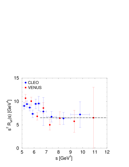
Figure 2: The scaled annihilation form factor $s^{2}R_{\rm eff}^{p}(s)$ as extracted from the data of [18, 20], using (47) with $R_{V}^{\,p}$ set to zero. The dashed line represents a fit to the data above $6.5\,~{}{\rm GeV}^{2}$.

Although a behavior of $R_{\rm eff}^{p}(s)\sim s^{-2}$ is compatible with experiment in the $s$ range we are investigating, a somewhat different falloff is not excluded by present experimental data. The $s$ dependence of our fitted annihilation form factor coincides with the one predicted by dimensional counting rules [28], as well as the corresponding behavior $d\sigma/dt\sim s^{-6}$ of the cross section (27) at fixed angle $\theta$. We emphasize that this does not imply the dominance of leading-twist contributions. It is also possible that, in a way similar to wide-angle Compton scattering [7, 15], dimensional counting rule behavior is mimicked by soft physics over a large yet finite range of $s$. From our calculation of the handbag diagrams it is clear that the form factors appearing in (3) are only the soft parts of the matrix elements $R_{i}(s)$ ($i=V,\,A,\,P$) defined by (5) and (26). According to general power counting arguments, the soft parts of $R_{V}$, $R_{A}$ and $\sqrt{s}\,R_{P}$ will decrease faster than $s^{-2}$ for very large $s$. The soft handbag contribution to the cross section $d\sigma/dt$ then falls off faster than $s^{-6}$ at fixed $\theta$, and the hard leading-twist contribution will eventually dominate. We remark that in the spacelike region one can use a model based on wave function overlap to evaluate the soft parts of the Compton form factors $R_{V}(t)$ and $R_{A}(t)$ [7]. Their asymptotic behavior in this model is a decrease like $t^{-4}$ and only sets in for $-t$ of order 100 GeV².

We observe that the annihilation form factor (48) is of similar size as the time-like magnetic form factor of the proton. The situation is thus similar to the space-like region, where the Dirac form factor and the form factors for wide-angle Compton scattering off the proton also behave similarly and are of comparable magnitude [7, 15]. Recall that the Compton form factors $R_{A}$ and $R_{V}$ are given by moments in $x$ of generalized parton distributions whose respective forward limits are the polarized and unpolarized quark densities $\Delta q$ and $q$. If one assumes that at large $x$ these generalized parton distributions have the same $x$-dependence as their forward limits, up to a common factor $f(x,t)$ for both distributions, one obtains $|R_{A}(t)|\leq R_{V}(t)$ at large $t$ as a consequence of the positivity bound $|\Delta q|\leq q$. For generalized distribution amplitudes there is no such constraint, and our estimates (44) and (50) suggest that one may indeed have $|R_{A}(s)|>|R_{V}(s)|$ for the annihilation form factors in the $s$-range of our fit.

Using the result (48) for $R_{\rm eff}^{p}$ we can now discuss the cross sections for other $B\overline{B}$ channels. In view of the large uncertainties of the data [19, 21] we do not attempt to include effects of flavor symmetry breaking and directly use the relations (43) to investigate the relative strength $\rho$ between $d\overline{d}\to p\overline{p}$ and $u\overline{u}\to p\overline{p}$ transitions. In Fig. 3 we show the cross sections for two-photon annihilation into $\Lambda\overline{\Lambda}$ and $\Sigma^{0}\overline{\Sigma}{}^{0}$ pairs, with the bands corresponding to the range

$$\rho=0.25\div 0.75\,.$$ (51)

According to our discussion in Sect. 4 such values are physically quite plausible. Values of $\rho$ significantly different from (51) are not favored by the data. The estimate (51) should of course be interpreted with due care, given theoretical uncertainties induced by the rather low $s$-values of the data (the respective production thresholds for $\Lambda\overline{\Lambda}$ and $\Sigma^{0}\overline{\Sigma}{}^{0}$ pairs are at $\sqrt{s}=2.23~{}~{}{\rm GeV}$ and $2.39~{}~{}{\rm GeV}$), the assumed $s$-dependence of $R_{\rm eff}^{p}$ in (48), and the simplifying assumptions that give the relations (43) between $B\overline{B}$ channels in terms of a single real-valued parameter $\rho$. We recall that the value in (51) essentially refers to the form factor combination $R_{\rm eff}^{p}\approx|R_{A}^{\,p}+R_{P}^{\,p}|$, which dominates the integrated cross section (47). Other $B\overline{B}$ channels can now easily be predicted from (43). A special role is played by the mixed channels $\Lambda\overline{\Sigma}{}^{0}$ and $\Sigma^{0}\overline{\Lambda}$, whose cross sections vanish at $\rho=1/2$. For these the estimate (51) provides an upper bound

$$\sigma(\Lambda\overline{\Sigma}{}^{0}+\Sigma^{0}\overline{\Lambda})\;\simeq\;\frac{3}{2}\,\left(\frac{1-2\rho}{4+\rho}\right)^{2}\sigma(p\overline{p})\;\leq\;0.02\;\sigma(p\overline{p})\,,$$ (52)

whose precise value should again be taken with care, given our discussion above.

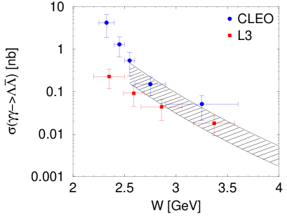
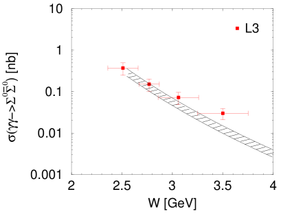
Figure 3: The cross sections for two-photon annihilation into $\Lambda\overline{\Lambda}$ (left) and $\Sigma^{0}\overline{\Sigma}{}^{0}$ pairs (right) versus $W=\sqrt{s}$. Data is taken from [19, 21]. The bands correspond to the range $\rho=0.25\div 0.75$ in conjunction with the form factor $R_{\rm eff}^{p}(s)$ from (48), as explained in the text.

In Fig. 4 we show the angular distribution for $\gamma\gamma\to p\overline{p}$. Unfortunately, data exists only for rather small energies, where our kinematical requirements that $-t$ and $-u$ should be large compared to, say, the squared proton mass, can hardly be met. Furthermore, the influence of resonances may not yet be negligible, for which there might be a little hint in Fig. 4. At the energy of $\sqrt{s}\simeq 2.3~{}{\rm GeV}$ (not shown in the figure) the data of [18, 20] exhibit a maximum at $90^{\circ}$, which is a clear signal for the dominance of low partial waves and may be due to resonances. The comparison of the handbag result with the available data should therefore be interpreted with due caution. The curve in Fig. 4 shows the angular distribution of the handbag result when $R_{V}^{\,p}$ is neglected in (27). Taking our estimate (44) of $R_{V}^{\,p}$ for $\rho=0.5$, together with the result (48) for $R_{\rm eff}^{p}$, we get a change in the distribution that is too small to be seen in the figure. If on the other hand we take the value of $R_{V}^{\,p}$ which corresponds to $\rho=1$ in (44), the angular distribution becomes somewhat steeper. We emphasize however that the region where $-t$ or $-u$ is smaller than $1.5\,~{}{\rm GeV}^{2}$ corresponds to $|\cos\theta|>0.5$ for the data in Fig. 4. In this region the handbag result has to be taken with more than a grain of salt.

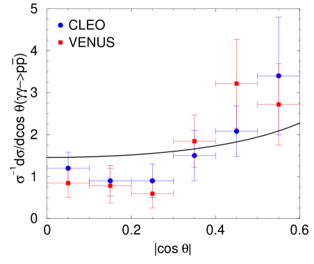
Figure 4: Normalized angular distribution of $\gamma\gamma\to p\overline{p}$ at $s=7.3~{}{\rm GeV}\,^{2}$. The solid line represents the handbag result (27) with the form factor $R_{V}^{\,p}$ neglected. Data is taken from [18, 20].

6 Concluding remarks

We have discussed the handbag contribution to two-photon annihilation into baryon-antibaryon pairs at large energy and large momentum transfer. Our main result is to write the amplitude as a product of a parton-level amplitude for $\gamma\gamma\to q\overline{q}$ and annihilation form factors given by moments of the $B\overline{B}$ distribution amplitudes. In our derivation we have to explicitly neglect contributions where the antiquark nearly takes the momentum of the baryon and the quark the momentum of the antibaryon. On the other hand, quark off-shell effects in the hard scattering and the bad components of the corresponding field operators are shown to be suppressed parametrically. An alternative treatment of the processes under investigation is possible using double distributions [29]. Our results also apply to the annihilation process $p\bar{p}\to\gamma\gamma$, whose form factors and amplitudes are related to those for two-photon annihilation by time reversal.

The factorization of the soft handbag diagrams is analogous to the one in wide-angle Compton scattering. For the latter it has been shown that this factorization remains valid when taking into account next-to-leading corrections in $\alpha_{\rm s}$ to the parton-level subprocess [11], and one may expect that the same holds for the time-like processes considered here.

The handbag contribution formally represents a power correction to the leading-twist hard-scattering mechanism, but it seems to dominate at experimentally accessible energies. We find that the data for various $B\overline{B}$ channels is compatible with annihilation form factors approximately behaving as $1/s^{2}$ for $s$ between $6$ and $12\,~{}{\rm GeV}^{\,2}$, a counting rule behavior typical of many exclusive observables. Fitting the form factors to the data, we find that for protons the sum of the axial and pseudoscalar annihilation form factors $R_{A}+R_{P}$ is dominant and somewhat larger than the time-like magnetic form factor. A further test of our approach is the approximate $1/\sin^{2}\theta$ angular dependence of the cross section, which agrees rather well with the VENUS data. According to our estimates, the $R_{V}$ term with its additional $\cos^{2}\theta$ dependences is likely too small to be seen in the presently available data. Flavor symmetry and the absence of $I=2$ components in the $q\overline{q}$ intermediate states relate $p\overline{p}$ production to the $B\overline{B}$ channels where $B$ is a member of the lowest lying baryon octet, up to presumably moderate effects of flavor SU(3) breaking. Fixing the relative strength $\rho$ of the form factors governing $d\overline{d}\to p\overline{p}$ and $u\overline{u}\to p\overline{p}$ transitions from suitable and sufficiently accurate data of two $B\overline{B}$ channels allows one to predict all other ones.

We emphasize that our comparison with experiment suffers from the low energies where data is currently available. For these energies the kinematical requirements of the handbag approach are hardly satisfied. Nevertheless we arrive at a satisfactory description of the data for the three channels $p\overline{p}$, $\Lambda\overline{\Lambda}$ and $\Sigma^{0}\overline{\Sigma}{}^{0}$, taking as soft physics input the effective form factor $R^{p}_{\rm eff}(s)$ and the flavor parameter $\rho$ with values in agreement with the physical interpretation of these quantities. We finally remark that measurement of the process $p\overline{p}\to\gamma\gamma$ with better statistics and at higher energies would likely be possible at the proposed HESR project at GSI [30].

Note added

After this work was finished, new data for the $p\bar{p}$ channel was published by OPAL [33]. In the high-$s$ range it agrees with the results from CLEO and VENUS we have referred to in Section 5.

Appendix: Spinor conventions

In our calculations we have used spinors for (anti)quarks and (anti)baryons that correspond to states with definite light-cone helicity [31]. In the usual Dirac representation they read

$$u(p,+) = N^{-1}\left(\begin{array}[]{c}p^{0}+p^{3}+m\\ p^{1}+ip^{2}\\ p^{0}+p^{3}-m\\ p^{1}+ip^{2}\end{array}\right),\qquad\hskip 8.00003ptu(p,-)\>=\>N^{-1}\left(\begin{array}[]{c}-p^{1}+ip^{2}\\ p^{0}+p^{3}+m\\ p^{1}-ip^{2}\\ -p^{0}-p^{3}+m\end{array}\right),$$ (61)

$$v(p,+) = N^{-1}\left(\begin{array}[]{c}p^{1}-ip^{2}\\ -p^{0}-p^{3}+m\\ -p^{1}+ip^{2}\\ p^{0}+p^{3}+m\end{array}\right),\qquad v(p,-)\>=\>N^{-1}\left(\begin{array}[]{c}-p^{0}-p^{3}+m\\ -p^{1}-ip^{2}\\ -p^{0}-p^{3}-m\\ -p^{1}-ip^{2}\end{array}\right),$$ (70)

where $N=\sqrt{2(p^{0}+p^{3})}$. This corresponds to the phase conventions used by Brodsky and Lepage, cf. [32], and also to those of Kogut and Soper [31] if one takes into account that they use a different representation of the Dirac matrices. The antiquark spinors in (61) satisfy the charge conjugation relations $v(p,\nu)=S(C)\,\overline{u}^{T}(p,\nu)$ with $S(C)=i\gamma^{2}\gamma^{0}$. For massless spinors one simply has $v(p,\nu)=-u(p,-\nu)$.

References

- [1] M. Diehl, P. Kroll and C. Vogt, Phys. Lett. B 532, 99 (2002) [hep-ph/0112274].
- [2] D. Müller, D. Robaschik, B. Geyer, F. M. Dittes and J. Hořejši, Fortsch. Phys. 42, 101 (1994) [hep-ph/9812448].
- [3] M. Diehl, T. Gousset, B. Pire and O. Teryaev, Phys. Rev. Lett. 81, 1782 (1998) [hep-ph/9805380].
- [4] X. Ji, Phys. Rev. Lett. 78, 610 (1997) [hep-ph/9603249].
- [5] A. V. Radyushkin, Phys. Lett. B 380, 417 (1996) [hep-ph/9604317].
- [6] A. V. Radyushkin, Phys. Rev. D 58, 114008 (1998) [hep-ph/9803316].
- [7] M. Diehl, T. Feldmann, R. Jakob and P. Kroll, Eur. Phys. J. C 8, 409 (1999) [hep-ph/9811253].
- [8] G. P. Lepage and S. J. Brodsky, Phys. Rev. D 22, 2157 (1980).
- [9] A. Freund, Phys. Rev. D 61, 074010 (2000) [hep-ph/9903489].
-
[10]
M. V. Polyakov,
Nucl. Phys. B 555, 231 (1999)
[hep-ph/9809483];
M. Diehl, T. Gousset and B. Pire, Phys. Rev. D 62, 073014 (2000) [hep-ph/0003233]. - [11] H. W. Huang, P. Kroll and T. Morii, Eur. Phys. J. C 23, 301 (2002) [hep-ph/0110208].
-
[12]
O. Gayou et al. [Jefferson Lab Hall A Collaboration],
Phys. Rev. Lett. 88, 092301 (2002)
[nucl-ex/0111010];
M. K. Jones et al. [Jefferson Lab Hall A Collaboration], Phys. Rev. Lett. 84, 1398 (2000) [nucl-ex/9910005]. - [13] M. Diehl, Eur. Phys. J. C 19, 485 (2001) [hep-ph/0101335].
- [14] O. V. Teryaev, Phys. Lett. B 510, 125 (2001) [hep-ph/0102303].
- [15] M. Diehl, T. Feldmann, R. Jakob and P. Kroll, Phys. Lett. B 460, 204 (1999) [hep-ph/9903268].
- [16] B. A. Kniehl, G. Kramer and B. Pötter, Nucl. Phys. B 582, 514 (2000) [hep-ph/0010289].
- [17] T. Sjöstrand et al., Comput. Phys. Commun. 135, 238 (2001) [hep-ph/0010017].
- [18] M. Artuso et al. [CLEO Collaboration], Phys. Rev. D 50, 5484 (1994).
- [19] S. Anderson et al. [CLEO Collaboration], Phys. Rev. D 56, 2485 (1997) [hep-ex/9701013].
- [20] H. Hamasaki et al. [VENUS Collaboration], Phys. Lett. B 407, 185 (1997).
- [21] P. Achard et al. [L3 Collaboration], Phys. Lett. B 536, 24 (2002) [hep-ex/0204025].
- [22] G. R. Farrar, E. Maina and F. Neri, Nucl. Phys. B 259, 702 (1985) [Erratum-ibid. B 263, 746 (1985)].
-
[23]
J. Bolz and P. Kroll,
Z. Phys. A 356, 327 (1996)
[hep-ph/9603289];
V. M. Braun, A. Lenz, N. Mahnke and E. Stein, Phys. Rev. D 65, 074011 (2002) [hep-ph/0112085];
D. Diakonov and V. Y. Petrov, hep-ph/0009006. -
[24]
P. Kroll, T. Pilsner, M. Schürmann and W. Schweiger,
Phys. Lett. B 316, 546 (1993)
[hep-ph/9305251];
C. F. Berger, B. Lechner and W. Schweiger, FizikaB 8, 371 (1999) [hep-ph/9901338]. -
[25]
M. Diehl, T. Feldmann, R. Jakob and P. Kroll,
Nucl. Phys. B 596, 33 (2001),
Erratum-ibid. B 605, 647 (2001)
[hep-ph/0009255];
S. J. Brodsky, M. Diehl and D. S. Hwang, Nucl. Phys. B 596, 99 (2001) [hep-ph/0009254]. - [26] B. C. Tiburzi and G. A. Miller, hep-ph/0205109.
- [27] T. A. Armstrong et al. [E760 Collaboration], Phys. Rev. Lett. 70, 1212 (1993).
-
[28]
S. J. Brodsky and G. R. Farrar,
Phys. Rev. Lett. 31, 1153 (1973);
V. A. Matveev, R. M. Muradian and A. N. Tavkhelidze, Lett. Nuovo Cim. 7, 719 (1973). - [29] A. Freund, A. V. Radyushkin, A. Schäfer and C. Weiss, hep-ph/0208061.
- [30] An International Accelerator Facility for Beams of Ions and Antiprotons, Conceptual Design Report, GSI Darmstadt, November 2001.
- [31] J. B. Kogut and D. E. Soper, Phys. Rev. D 1, 2901 (1970).
- [32] S. J. Brodsky, H. C. Pauli and S. S. Pinsky, Phys. Rept. 301, 299 (1998) [hep-ph/9705477].
- [33] G. Abbiendi et al. [OPAL Collaboration], hep-ex/0209052.