KUNS-1794

HUPD-0203

Schwinger-Dyson Analysis of Dynamical Symmetry Breaking on a Brane with Bulk Yang-Mills Theory

Hiroyuki Abe^∗,†, and  Tomohiro Inagaki^§,

^∗Department of Physics, Kyoto University, Kyoto 606-8502, Japan

^†Department of Physics, Hiroshima University, Hiroshima 739-8526, Japan

^§Information Media Center, Hiroshima University, Hiroshima 739-8521, Japan

The dynamically generated fermion mass is investigated in the flat brane world with $(4+\delta)$-dimensional bulk space-time, and in the Randall-Sundrum (RS) brane world. We consider the bulk Yang-Mills theory interacting with the fermion confined on a four-dimensional brane. Based on the effective theory below the reduced cutoff scale on the brane, we formulate the Schwinger-Dyson equation of the brane fermion propagator. By using the improved ladder approximation we numerically solve the Schwinger-Dyson equation and find that the dynamical fermion mass is near the reduced cutoff scale on the brane for the flat brane world with $\delta\geq 3$ and for the RS brane world. In RS brane world KK excited modes of the bulk gauge field localized around the $y=\pi R$ brane and it enhances the dynamical symmetry breaking on the brane. The decay constant of the fermion and the anti-fermion composite operator can be taken to be the order of the electroweak scale much smaller than the Planck scale. Therefore electroweak mass scale can be realized from only the Planck scale in the RS brane world due to the fermion and the anti-fermion pair condensation. That is a dynamical realization of Randall-Sundrum model which solves the weak-Planck hierarchy problem.

1 Introduction

Up to the energy scale we can test experimentally, the standard model (SM) well describes the forces between matter particles except for the gravity. Almost all the candidates for the theory of the gravity at Planck scale $M_{\rm Pl}$ are defined with the supersymmetry (SUSY) in more than 4-dimensional (4D) space-time, such as supergravity or superstring theory. It is considered that the SM particles lie in higher dimensional space-time and extra dimensions are compactified smaller than the size we can detect in the low energy experiments or lie on the 4D subspace in higher dimensional space-time. Recent interesting suggestion is that SM may be realized on a ‘brane’ which stands for the lower dimensional object in the higher dimensional space-time. One of the candidates of such object is D-brane or domain wall. We call such scenario ‘brane world model.’ The brane world models now casting new ideas on physics beyond the SM. For example recent studies in the superstring theory provide us some concrete examples realizing SM in the D-brane systems [1].

Basis of the SM is a spontaneous gauge symmetry breaking that results in the existence of the massive gauge bosons, W and Z. We need at least one (doublet) scalar field, called Higgs field which develops a vacuum expectation value (VEV) to give a masses to the W and Z gauge bosons and breaks the SM gauge symmetry. These gauge boson masses are related to the electroweak scale $M_{\rm EW}$ at which the SM gauge symmetry is broken as $SU(3)_{c}\times SU(2)_{L}\times U(1)_{Y}\to SU(3)_{c}\times U(1)_{EM}$. The mass scale of the W and Z gauge bosons shows that $M_{\rm EW}$ is of the order TeV scale, while the gravitational scale, namely Planck scale $M_{\rm Pl}$ is of the order $10^{19}$ GeV. If we consider the unification of SM and gravity, we should explain the hierarchical structure between $M_{\rm Pl}$ and $M_{\rm EW}$. Since the mass of the scalar field is not protected by any symmetries, the radiative correction brings the Higgs mass to the fundamental scale $M_{\rm Pl}$ without a fine tuning. This is so called ‘hierarchy’ or ‘fine tuning’ problem. There are two remarkable brane world models solving this hierarchy problem. One is the large extra dimension scenario [2] and the other is the warped extra dimension scenario in Randall-Sundrum (RS) brane world [3].

SUSY enables to stabilize the scalar mass against the radiative correction of ${\cal O}(M_{\rm Pl})$ because it is related to the mass of the fermionic superpartner that can be protected by appropriate symmetry. So the SUSY permits the light scalar field like Higgs field, however if we introduce it around the TeV scale in order to keep the Higgs mass $\sim$ TeV, all the fermions in the SM have their scalar partners with their masses around TeV. These extra scalar fields have not been observed in any experiments yet. Thus we need some mechanisms in the SUSY breaking process to control these extra light scalars not to appear inside the region of the present experimental observation. However, the supertrace theorem predicts lighter scalar partners than the fermions in SM that is not consistent with the experimental results. To avoid this problem the theory should have the ‘hidden sector’ where SUSY is broken. A certain mediation mechanism to communicate it to the ‘visible sector’ is required at the loop level through renormalizable interactions or at the tree level through unrenormalizable interactions. Recently some people consider that the hidden sector setup merges into the brane world picture, that separates the hidden and visible sector by spatiality in the extra dimension. They use the bulk (moduli) fields to communicate the SUSY breaking signals from the hidden to the visible sector [4]. The hidden sector is the minimal requirement from the supertrace theorem and we need more severe conditions to the SUSY breaking from the experiment. One of them is from the supersymmetric flavor problem, that is the masses of the SM fermions are disjointed each other while the masses of their scalar partners are almost degenerate.

As we see above almost all the problems in the TeV scale SUSY come from too much light extra fields in addition to the SM one. We need complicated setup about SUSY breaking (and its mediation) mechanism to avoid these problems. Remember that SUSY itself is needed for the consistency of the quantum theory of gravity, while ‘TeV scale SUSY’ is required in order to stabilize the electroweak scale $M_{\rm EW}$, and to realize gauge coupling unification. However, in a recent brane world picture, there is a possibility that the strong and electroweak gauge group come from the different brane. In this case the unification of SM and gravity is able to occur directly without grand unification and the gauge coupling unification in MSSM may be accidental. We can also consider the case that gauge coupling unification is not depend on the TeV scale SUSY (MSSM) and it happens by the other mechanism, e.g. extra dimensional effect [5, 6]. If there is another mechanism to stabilize mass of the Higgs field, it is possible to break SUSY at higher energy scale, even around the Planck scale. Such a mechanism can set SUSY free from any problems at TeV scale.

In this paper we notice the recent suggestions that the electroweak (chiral) symmetry is broken down dynamically by the gauge interaction in more than 4D space-time [7, 8, 9, 10, 11]. The higher dimensional gauge theory may realize the stabilization of a light Higgs field through the composite Higgs scenario. This is based on the idea that the gauge theory in compact extra dimension has Kaluza-Klein (KK) massive gauge bosons and they act as a binding force between fermion and anti-fermion that results in the composite scalar field. It was pointed out in Refs. [12] and [13] a negative curvature and a finite size effects enhance dynamical symmetry breaking. If SM is embedded in a brane world, the dynamical mechanism of electroweak symmetry breaking can be realized in a certain bulk gauge theory (or SM itself in the bulk.) SM in the bulk has a possibility to realize top quark condensation scenario [15] in the brane world. It is very interesting because it may have no extra field (elementary Higgs, techni-color gauge boson, techni-fermion etc.) except for the SM contents (without elementary Higgs) in order to break the electroweak symmetry. We launched a plan to study the dynamical symmetry breaking in the brane world models in detail.

There is no enough knowledge about the (non-perturbative) dynamics of the higher dimensional gauge theory in brane world. In this paper we study the basic properties of dynamical symmetry breaking in the bulk gauge theory couples to a fermion on the brane. Based on the effective theory of the bulk Yang-Mills theory that is defined below the reduced cutoff scale on the brane, we formulate the ladder Schwinger-Dyson (SD) equation of the fermion propagator. It is numerically solved by using the improved ladder approximation with power low running of the effective gauge coupling. We show how the dynamics of the bulk gauge field affects the chiral symmetry breaking on the brane.

We give a KK reduced Lagrangian of our bulk-brane system in $\S$2. In $\S$3 we derive the effective theory on the four-dimensional brane and formulate SD equation about the fermion propagator on the brane. The Numerical analysis of the SD equation is performed, within the improved ladder approximation, for the case of Yang-Mills theory on the brane, in the flat bulk space-time and in the warped bulk space-time in $\S$4.

2 Lagrangian of the System

In this paper we analyze dynamical symmetry breaking on the four dimensional brane with bulk gauge theory in various brane world models. The bulk gauge theory is, of course, more than four dimensional theory and ill defined in ultraviolet (UV) region and we need some regularization about it. In this paper we use effective Lagrangian of it defined below the reduced cutoff scale on the brane.

In this section we derive the KK reduced 4D Lagrangian of the bulk gauge theory in the brane worlds, $M_{4}\times S^{1}$ type space-time. We can easily extend it to the case of higher dimensional bulk space-time, $M_{4}\times T^{\delta}$, it is shown in the next section. Because one of our goal is to analyze the dynamically induced mass scale on the brane in the Randall-Sundrum space-time, i.e. the slice of AdS₅, we take account for the Lagrangian and mode function in a curved extra dimension. The original motivation to introduce a curved extra dimension by Randall and Sundrum is to produce the weak-Planck hierarchy from the exponential factor in the space-time metric. The factor is called ‘warp factor’, and the extra space ‘warped extra dimension’. A non-factorizable geometry with the warp factor distinguishes the RS brane world from the others. In the RS model we consider the fifth dimension $y$ which is compactified on an orbifold, $S^{1}/Z_{2}$ of radius $R$ and two 3-branes at the orbifold fixed points, $y^{\ast}=0$ and $\pi R$. Requiring the bulk and boundary cosmological constants to be related, Einstein’s equation in five-dimension leads to the solution [3],

$$ds^{2}=G_{MN}dx^{M}dx^{N}=e^{-2k|y|}\eta_{\mu\nu}dx^{\mu}dx^{\nu}-dy^{2},$$ (1)

where $M,N$ = $0,1,2,3,4$, $\mu,\nu=0,1,2,3$ and $\eta_{\mu\nu}={\rm diag}(1,-1,-1,-1)$. $k$ is the AdS curvature scale with the mass dimension one, and $k=0$ describes the flat $M_{4}\times S^{1}$ space-time. In the following we study a bulk vector field, $A_{M}$ in this background.

2.1 KK Reduced Lagrangian of Bulk Gauge Theory

Substituting the metric $G_{MN}$ defined in Eq. (1) and taking $A_{4}=0$ gauge, the Lagrangian of a bulk gauge field in the RS brane world is written by

$${\cal L}_{\rm gauge}^{(5)}=-\frac{1}{4}\sqrt{-G}F^{MN}F_{MN}=-\frac{1}{4}F^{\mu\nu}F_{\mu\nu}+\frac{1}{2}e^{-2k|y|}(\partial_{4}A_{\mu})^{2}+{\cal L}_{\rm SI}^{(5)},$$ (2)

where ${\cal L}_{\rm SI}^{(5)}$ includes the gluon three and four point self interaction in the bulk. We drop the explicit symbol of the trace operation in terms of the Yang-Mills index in the Lagrangian throughout this paper. We perform the KK mode expansion as

$$A_{\mu}(x,y)=\frac{1}{\sqrt{2\pi R}}\left(\sum_{n=0}^{\infty}A_{\mu}^{(n)}(x)\chi_{n}(y)+\sum_{n=1}^{\infty}\tilde{A}_{\mu}^{(n)}(x)\tilde{\chi}_{n}(y)\right),$$ (3)

where $\chi_{n}(y)$ and $\tilde{\chi}_{n}(y)$ are the $Z_{2}$ even and odd mode function of $n$-th KK excited mode $A_{\mu}^{(n)}(x)$ and $\tilde{A}_{\mu}^{(n)}(x)$, respectively. The $Z_{2}$ orbifold condition thus means $\tilde{A}_{\mu}^{(n)}(x)\equiv 0$ for ${}^{\forall}n$, i.e. dropping all the odd modes. After KK expansion, we integrate the Lagrangian (2) over the y-direction and obtain

$${\cal L}_{\rm gauge} = \sum_{n=0}^{\infty}\left[-\frac{1}{4}F^{(n)\mu\nu}(x)F_{\mu\nu}^{(n)}(x)+\frac{1}{2}M_{n}^{2}A^{(n)\mu}A_{\mu}^{(n)}\right]$$ (4)

$$+\sum_{n=1}^{\infty}\left[-\frac{1}{4}\tilde{F}^{(n)\mu\nu}(x)\tilde{F}_{\mu\nu}^{(n)}(x)+\frac{1}{2}M_{n}^{2}\tilde{A}^{(n)\mu}\tilde{A}_{\mu}^{(n)}\right],$$

where the KK mode function $\chi_{n}(y)$ and mass eigenvalue $M_{n}$ satisfy

$$-\partial_{y}\left(e^{-2k|y|}\partial_{y}\chi_{n}(y)\right) = M_{n}^{2}\chi_{n}(y),$$ (5)

$$\frac{1}{2\pi R}\int_{-\pi R}^{\pi R}dy\,\chi_{n}(y)\chi_{m}(y) = \delta_{nm},$$ (6)

and $\tilde{\chi}_{n}(y)$ obeys the same equations. The boundary conditions are given by

$$\partial_{y}\chi_{n}(y^{\ast})=\tilde{\chi}_{n}(y^{\ast})=0\qquad(y^{\ast}=0,\pi R).$$ (7)

Eq. (4) is the 4D effective Lagrangian of the bulk gauge theory and Eqs. (5)-(7) determine the form of the mode function and the eigenvalue $M_{n}$. Below we solve Eq. (5) with the boundary condition (7) and the normalization (6) for the flat ($k=0$) and warped ($k\neq 0$) extra dimensions.

We call the case with $k=0$ ‘flat brane world’. In this case the solution of Eqs. (5)-(7) is given by

$$\chi_{0}(y) = 1,$$ (8)

$$\chi_{n}(y) = \sqrt{2}\cos(ny/R)\quad(n=1,2,\ldots),$$ (9)

$$\tilde{\chi}_{n}(y) = \sqrt{2}\sin(ny/R)\quad(n=1,2,\ldots),$$ (10)

$$M_{n} = n\mu_{R},$$ (11)

where $\mu_{R}=1/R$. These are the KK mode function and mass eigenvalue of the bulk gauge field in the flat brane world with $M_{4}\times S^{1}$. We can easily extend it to higher dimensional bulk space-time, $M_{4}\times T^{\delta}$, that is shown latter.

$k\neq 0$ with orbifold condition, $\tilde{A}_{\mu}^{(n)}(x)\equiv 0$ for ${}^{\forall}n$, gives the RS brane world. The solution of Eqs. (5)-(7) reads [16]

$$\chi_{0}(y) = 1,$$ (12)

$$\chi_{n}(y) = \frac{e^{k|y|}}{N_{n}}\left[J_{1}\left(\frac{M_{n}}{k}e^{k|y|}\right)+c_{n}Y_{1}\left(\frac{M_{n}}{k}e^{k|y|}\right)\right]\quad(n=1,2,\ldots),$$ (13)

where the coefficient and the normalization factor are given by $c_{n}=-J_{0}\left(\frac{M_{n}}{k}\right)/Y_{0}\left(\frac{M_{n}}{k}\right)$ and $N_{n}^{2}=\frac{1}{2\pi R}\int_{-\pi R}^{\pi R}dy\,e^{2k|y|}\left[J_{1}\left(\frac{M_{n}}{k}e^{k|y|}\right)+c_{n}Y_{1}\left(\frac{M_{n}}{k}e^{k|y|}\right)\right]^{2}$ respectively and $J$ and $Y$ are the Bessel functions. The KK mass eigenvalue $M_{n}$ is obtained as the solution of $J_{0}\left(\frac{M_{n}}{k}\right)Y_{0}\left(\frac{M_{n}}{k}e^{\pi kR}\right)=Y_{0}\left(\frac{M_{n}}{k}\right)J_{0}\left(\frac{M_{n}}{k}e^{\pi kR}\right)$. For the case with $kR\gg 1$ and $M_{n}\ll k$ the asymptotic form of the KK mass eigenvalue is simplified to

$$M_{0} = 0,$$

$$M_{n} \simeq (n-1/4)\mu_{kR}\quad(n=1,2,\ldots),$$ (14)

where $\mu_{kR}\equiv\pi e^{-\pi kR}k$. We find that the spectrum of the excited mode is shifted by the factor $1/4$ and the mass difference between neighbour modes is suppressed by the warp factor $e^{-\pi kR}$. In the same asymptotic limit $n$-dependence of the mode function vanishes on the $y=\pi R$ brane. It reduces to

$$\chi_{n}(\pi R)\simeq\sqrt{2\pi kR}.$$ (15)

The profile of the mode functions $\chi_{n}(y)$ are shown in Fig. 1. From the figure we know that the KK excited gauge bosons are localized in the vicinity of the $y=\pi R$ brane in the RS brane world due to the finite curvature scale $k$ of the extra dimension, while the zero mode is flat in the direction of the extra dimension. We will see that the localized KK excited modes enhance (suppress) the dynamical symmetry breaking on the $y=\pi R$ ($y=0$) brane.

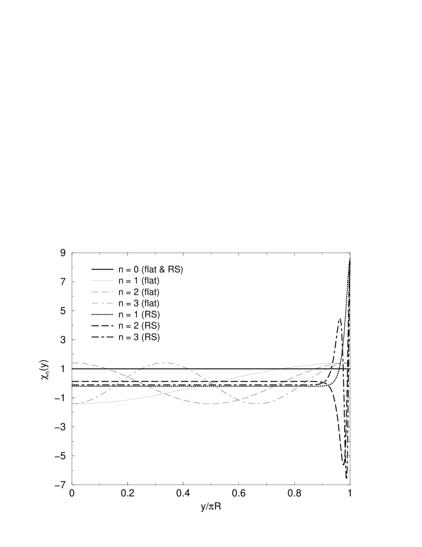
Figure 1: The profile of the mode functions $\chi_{n}(y)$ for $kR=11$, as a function of the coordinate of the extra dimension $y$. $\chi_{n}(y)$ are plotted so as to take a positive value at the $y/\pi R=1$.

2.2 Coupling to Brane Fermion

Next we define the coupling of the bulk gauge field to a fermion on the brane. By decomposing the metric as $G_{MN}=E_{\ M}^{\bar{M}}\eta_{\bar{M}\bar{N}}E_{\ N}^{\bar{N}}$ where $\eta_{\bar{M}\bar{N}}={\rm diag}(1,-1,-1,-1,-1)$, we define

$$E_{\bar{M}}^{\ M}=\left(\begin{array}[]{cc}e^{+k|y|}\delta_{\bar{\mu}}^{\ \mu}&0\\ 0&1\end{array}\right),\quad E_{\ M}^{\bar{M}}=\left(\begin{array}[]{cc}e^{-k|y|}\delta^{\bar{\mu}}_{\ \mu}&0\\ 0&1\end{array}\right),$$ (20)

where the row and column of the matrix correspond to the indices $M$ and $\bar{M}$ respectively. $E_{\bar{M}}^{M}$ gives the coupling of a fermion on the brane and the bulk gauge field. That is described as

$${\cal L}_{\rm coupling}^{(5)} = {(\det E_{\ \mu}^{\bar{\mu}})}^{-1}g_{\rm 5D}\bar{\Psi}(x)i\Gamma^{\bar{M}}E_{\bar{M}}^{\ M}(y)A_{M}(x,y)\Psi(x)\delta(y-y^{\ast})$$ (21)

$$= g_{\rm 5D}\bar{\Psi}(x)iA\!\!\!/(x,y)\Psi(x)\delta(y-y^{\ast}).$$

where $\Gamma_{\bar{M}}=(\gamma_{\mu},i\gamma_{5})$, $A\!\!\!/=\gamma^{\mu}A_{\mu}$, $g_{\rm 5D}$ is the five dimensional gauge coupling and $y^{\ast}$ is the position of the brane. In the second line we take $A_{4}=0$ gauge and rescale $\Psi$ field as $\Psi\to e^{3k|y^{\ast}|/2}\Psi$ in order to canonically normalize the kinetic term of $\Psi$. By integrating (21) over the extra dimensional coordinate we obtain the 4D effective gauge coupling written by

$${\cal L}_{\rm coupling} = \sum_{n=0}^{\infty}g_{n}\bar{\Psi}(x)i{A\!\!\!/}^{(n)}(x)\Psi(x)+\sum_{n=1}^{\infty}\tilde{g}_{n}\bar{\Psi}(x)i{\tilde{A}\!\!\!/}^{(n)}(x)\Psi(x),$$ (22)

where

$$g_{n}=\frac{\chi_{n}(y^{\ast})}{\chi_{0}(y^{\ast})}g_{0},\quad g_{0}=\frac{\chi_{0}(y^{\ast})}{\sqrt{2\pi R}}g_{\rm 5D}\equiv g,$$ (23)

where $g$ is the ordinary four dimensional gauge coupling. $\tilde{g}_{n}$ is defined by replacing $\chi$ with $\tilde{\chi}$ in Eq. (23). In the case $y^{\ast}=0,\pi R$, i.e. $\tilde{g}_{n}=0$ (see Eq. (7)), $\tilde{A}_{\mu}^{(n)}(x)$ decouples in Eq. (22). We notice that the coupling of the gauge boson excited modes $g_{n}$ are enhanced/suppressed by the value of the mode function $\chi_{n}$ on the $y=y^{\ast}$ brane, compared with it of zero mode. Thus we obtain larger effect from the KK excited gauge boson on the brane they localize.

3 Effective Theory and Schwinger-Dyson Equation on a Brane

In the previous section we have derived the Lagrangian of the bulk gauge field and its coupling to a fermion on the brane. Putting them together we obtain the effective Lagrangian for the system of the bulk gauge theory couples to fermion on the $y=y^{\ast}(=0,\pi R)$ brane as

$${\cal L} = \frac{1}{2}\sum_{n=0}^{N_{\rm KK}}A_{\mu}^{(n)}\left[\eta^{\mu\nu}\left(\partial^{2}+M_{n}^{2}\right)-(1-\xi)\partial_{\mu}\partial_{\nu}\right]A_{\nu}^{(n)}$$ (24)

$$+\frac{1}{2}\sum_{n=1}^{N_{\rm KK}}\tilde{A}_{\mu}^{(n)}\left[\eta^{\mu\nu}\left(\partial^{2}+M_{n}^{2}\right)-(1-\xi)\partial_{\mu}\partial_{\nu}\right]\tilde{A}_{\nu}^{(n)}+{\cal L}_{\rm SI}$$

$$+\bar{\Psi}\left(i\partial_{\mu}+gA_{\mu}^{(0)}\right)\gamma^{\mu}\Psi+g\sum_{n=1}^{N_{\rm KK}}\frac{\chi_{n}(y^{\ast})}{\chi_{0}(y^{\ast})}\bar{\Psi}A_{\mu}^{(n)}\gamma^{\mu}\Psi,$$

where ${\cal L}_{\rm SI}$ represents the self interaction (and mixing) terms of $A_{\mu}^{(n)}$ and $\tilde{A}_{\mu}^{(n)}$, and $N_{\rm KK}$ stands for the cutoff of the KK summation. It should be noted that we introduce the gauge fixing parameter $\xi$ on the brane. (See appendix in Ref. [11] for more details.) $\xi$ is chosen so that a QED like Ward-Takahashi identity is hold in the latter analysis. We can easily extend the above system to higher dimensional bulk space-time with $M_{4}\times T^{\delta}$ by replacing $M_{n}$ and $\chi_{n}$ as

$$M_{n} \to \sqrt{M_{n_{1}}^{2}+M_{n_{2}}^{2}+\ldots+M_{n_{\delta}}^{2}},$$ (25)

$$\chi_{n}(y) \to \chi_{n_{1}}(y_{1})\chi_{n_{2}}(y_{2})\cdots\chi_{n_{\delta}}(y_{\delta}),$$ (26)

where $n_{1},n_{2},\ldots,n_{\delta}=0,1,2,\ldots$ correspond to the indices of the KK excited mode for each extra dimension $(y_{1},y_{2},\ldots,y_{\delta})$ respectively. $M_{n_{i}}$ and $\chi_{n_{i}}(y_{i})$ $(i=1,...,\delta)$ are given in Eqs. (9) and (11) respectively. In addition we should interpret $\sum_{n}$ as $\sum_{n_{1}}\sum_{n_{2}}\cdots\sum_{n_{3}}$ with a cut-off condition, $n^{2}=n_{1}^{2}+n_{2}^{2}+\ldots+n_{\delta}^{2}\leq N_{\rm KK}^{2}$.

In the following discussion we regard the KK reduced Lagrangian (24) as an effective one below the bulk fundamental scale $\Lambda_{\rm 5D}$. Thus we cutoff the momentum of the loop integral, including only the propagator of bulk fields, at the scale $\Lambda_{\rm 5D}$. On the other hand we cutoff the momentum at the reduced cutoff scale $\Lambda$ on the brane in the case that the loop integral includes the brane fields. Loop integrals in the ladder Schwinger-Dyson equation is only the latter case. In the flat brane world $\Lambda$ should be the same order of $\Lambda_{\rm 5D}$, while in the RS brane world we have an large difference between $\Lambda$ and $\Lambda_{\rm 5D}$ due to the warp factor. We also define $N_{\rm KK}$ as the number of the KK modes with their mass below the reduced cutoff scale $\Lambda$. In our numerical analyses, however, we cutoff the KK mode summation at $N_{\rm KK}+10$ in order to avoid the sharp threshold effect.

From the Lagrangian (24) we construct a Schwinger-Dyson equation for the fermion propagator,

$$iS^{-1}(p)=iS^{-1}_{0}(p)+\sum_{n=0}^{N_{\rm KK}}\int\frac{d^{4}q}{i(2\pi)^{4}}\left[-ig_{n}T^{a}\Gamma^{M}\right]S(q)\left[-ig_{n}T^{a}\Gamma^{N}\right]D_{MN}^{(n)}(p-q),$$ (27)

where $T^{a}$ is the gauge group representation matrix of the fermion, and $S_{0}(p)=i/p\!\!\!/$, $S(p)$ and $D_{MN}^{(n)}(p-q)$ are the free fermion propagator, full fermion propagator and full $n$-th excited KK gauge boson propagator respectively. In this paper we use the (improved) ladder approximation in which $D_{MN}^{(n)}$ is replaced by the free propagator,

$$D_{MN}^{(n)}(k) \equiv \frac{-i}{k^{2}-M_{n}^{2}}\left[\eta_{MN}-(1-\xi)\frac{k_{M}k_{N}}{k^{2}-\xi M_{n}^{2}}\right].$$ (28)

By writing the full fermion propagator as

$$iS^{-1}(p) \equiv A(-p^{2})p\!\!\!/-B(-p^{2}),$$ (29)

the SD equation (27) becomes the simultaneous integral equation of $A$ and $B$,

$$A(p^{2}) = 1+\int_{0}^{\Lambda^{2}}dq^{2}\,\frac{q^{2}A(q^{2})}{A^{2}(q^{2})q^{2}+B^{2}(q^{2})}\sum_{n=0}^{N_{\rm KK}}L_{\xi}(p^{2},q^{2};M_{n},\alpha_{n}),$$ (30)

$$B(p^{2}) = \int_{0}^{\Lambda^{2}}dq^{2}\,\frac{q^{2}B(q^{2})}{A^{2}(q^{2})q^{2}+B^{2}(q^{2})}\sum_{n=0}^{N_{\rm KK}}K_{\xi}(p^{2},q^{2};M_{n},\alpha_{n}),$$ (31)

where

$$L_{\xi}(p^{2},q^{2};M_{n},\alpha_{n}) = \frac{\alpha_{n}}{4\pi}\Bigg{[}q^{2}f_{M_{n}^{2}}^{2}(p^{2},q^{2})+\frac{2q^{2}}{M_{n}^{2}}\left\{f_{M_{n}^{2}}(p^{2},q^{2})-f_{\xi M_{n}^{2}}(p^{2},q^{2})\right\}$$ (32)

$$\hskip 28.45274pt-\frac{(q^{2})^{2}+p^{2}q^{2}}{2M_{n}^{2}}\left\{f_{M_{n}^{2}}^{2}(p^{2},q^{2})-f_{\xi M_{n}^{2}}^{2}(p^{2},q^{2})\right\}\Bigg{]},$$

$$K_{\xi}(p^{2},q^{2};M_{n},\alpha_{n}) = \frac{\alpha_{n}}{4\pi}\bigg{[}4f_{M_{n}^{2}}(p^{2},q^{2})+\frac{p^{2}+q^{2}}{M_{n}^{2}}\left\{f_{M_{n}^{2}}(p^{2},q^{2})-f_{\xi M_{n}^{2}}(p^{2},q^{2})\right\}$$ (33)

$$\hskip 28.45274pt-\frac{p^{2}q^{2}}{M_{n}^{2}}\left\{f_{M_{n}^{2}}^{2}(p^{2},q^{2})-f_{\xi M_{n}^{2}}^{2}(p^{2},q^{2})\right\}\Bigg{]},$$

$$f_{M}(p^{2},q^{2}) = \frac{2}{p^{2}+q^{2}+M+\sqrt{(p^{2}+q^{2}+M)^{2}-4p^{2}q^{2}}},$$ (34)

$$\alpha_{n} \equiv \alpha\chi_{n}^{2}(y^{\ast})\qquad(n\neq 0),$$ (35)

$$\alpha_{0} = \alpha=g^{2}/4\pi.$$ (36)

Since our analysis is based on the effective theory on the four-dimensional brane below the reduced cutoff, the explicit UV cutoff $\Lambda$ in terms of the loop momentum on the brane appears. $A(x)$ and $B(x)$ are the wave function normalization factor and the mass function of the fermion respectively. The mass function $B(x)$ is the oder parameter of chiral symmetry breaking on the brane. The chiral symmetry is broken down for $B(x)\neq 0$. By solving Eqs. (30) and (31) we obtain the behavior of the dynamical fermion mass on the brane.

4 Improved Ladder Analysis of Dynamical Mass on the Brane

In this section we numerically solve the SD equation and analyze dynamical brane fermion mass induced by the bulk gauge theory. In the case of the bulk Abelian gauge theory with $N_{\rm KK}\lesssim 10$ we can use the point vertex approximation and the results are shown in [11]. In this section we extend the analysis in [11] to the bulk Yang-Mills theory. To solve the SD equation of Yang-Mills theory we use the improved ladder approximation where the running coupling is imposed to the vertex function. The running coupling is derived from the truncated KK approach proposed in Ref. [5]. We use the asymptotic form (14) of the KK spectrum to evaluate the running coupling in RS brane world.

First we review the process of analyzing SD equation in usual 4D QCD [17], and then we extend it to the brane world bulk Yang-Mills theory. For convenience we choose bulk QCD ($SU(3)_{c}$ Yang-Mills theory with $N_{\rm f}=3$ flavor fermion on the brane) as a concrete example because its results can be compared with the usual 4D QCD. We expect that the essential point of the results is not changed in the other bulk Yang-Mills theory such as techni-color.

4.1 QCD on the Brane (Usual 4D QCD)

Taking $N_{\rm KK}=0$ in Eqs. (30) and (31), the SD equation for usual QCD in four dimensional space-time (i.e. QCD on the brane) is obtained. In this case the integration kernels (32) and (33) become

$$L_{\xi}(p^{2},q^{2};M_{0}=0,\alpha_{0}=\alpha) = \frac{\alpha}{4\pi}\,\xi\,q^{2}\,f_{0}^{2}(p^{2},q^{2}),$$ (37)

$$K_{\xi}(p^{2},q^{2};M_{0}=0,\alpha_{0}=\alpha) = \frac{\alpha}{4\pi}\,(3+\xi)\,f_{0}(p^{2},q^{2}),$$ (38)

where

$$f_{0}(p^{2},q^{2}) = \theta(p^{2}-q^{2})\frac{1}{p^{2}}+\theta(q^{2}-p^{2})\frac{1}{q^{2}}.$$ (39)

We usually use Landau gauge $\xi=0$ that results in $L_{\xi}(p^{2},q^{2};M_{0}=0,\alpha_{0}=\alpha)=0$, i.e. $A(p^{2})=1$ in the SD equation. In that case the SD equation becomes single equation only with $B(p^{2})$. $A(p^{2})=1$ satisfies the QED like Ward-Takahashi identity.

We put the running coupling on the vertex function in the SD equation to compensate for neglecting three and four point gluon self interactions ${\cal L}_{\rm SI}$ in the ladder approximation. That is so called improved ladder approximation. We use the 1-loop perturbative running coupling,

$$\alpha\equiv\frac{\pi}{3C_{2}(F)}\lambda(k^{2}),$$ (40)

where

$$\lambda(z) = \frac{\lambda_{0}}{1+\lambda_{0}B\ln\frac{z}{\mu^{2}}},$$ (41)

and $B=\frac{4\pi^{2}}{3C_{2}(F)}\beta_{0}$. We define $\beta_{0}$ by $\beta(g)=-\beta_{0}g^{3}+{\cal O}(g^{5})$ and $\beta_{0}=\frac{1}{16\pi^{2}}\big{[}\frac{11}{3}C_{2}(G)-\frac{4}{3}N_{\rm f}T(F)\big{]}$ where $G$ and $F$ stand for the gauge group and the fermion representation under the group respectively. $C_{2}(G)$, $C_{2}(F)$ and $T(F)$ are defined by $\sum_{c,d}f_{acd}f_{bcd}\equiv C_{2}(G)\delta_{ab}$, $\textrm{tr}(T^{a}T^{b})\equiv T(F)\delta_{ab}$ and $\sum_{a}T^{a}T^{a}\equiv C_{2}(F)1$. In the case that $G=SU(N=3)$ and $F$ is fundamental representation, these values are given by

$$C_{2}(G)=N=3,\quad T(F)=\frac{1}{2},\quad C_{2}(F)=\frac{N^{2}-1}{2N}=4/3,$$ (42)

$$B=\frac{1}{12C_{2}(F)}\left(\frac{11N-2N_{\rm f}}{3}\right)=\frac{9}{16},\quad(N=3,N_{\rm f}=3).$$ (43)

We also define $\Lambda_{\rm QCD}$, the dynamical scale of QCD, as

$$\frac{1}{\lambda(z)}-B\ln z=\frac{1}{\lambda_{0}}-B\ln\mu^{2}\ \equiv\ -B\ln\Lambda_{\rm QCD}^{2},\qquad\left(\Lambda_{\rm QCD}^{2}\equiv\mu^{2}/e^{\frac{1}{\lambda_{0}B}}\right),$$ (44)

and obtain

$$\lambda(z) = \frac{16}{9}\frac{1}{\ln(z/\Lambda_{\rm QCD}^{2})}.$$ (45)

Following the analysis in Ref. [18] we introduce IR cutoff $z_{\rm IF}$ in the running coupling as

$$\alpha(z) = \frac{\pi}{3C_{2}(F)}\left[\theta(z_{\rm IF}-z)\lambda(z_{\rm IF})+\theta(z-z_{\rm IF})\lambda(z)\right],$$ (46)

and we take the following approximation

$$\alpha \to \alpha(z)\simeq\alpha(x+y),$$ (47)

in the integration kernel (37) and (38). It is called Higashijima-Miransky approximation. This is due to the consideration that the mean value of the $\theta$-dependent part in $\alpha(z)$ where $z=x+y-\sqrt{xy}\cos\theta$ has only a negligible effect after the angle integration in the SD equation. It is known that the approximation (47) violates the chiral Ward-Takahashi identity. In the present paper we choose the gauge parameter $\xi$ to nearly hold the chiral Ward-Takahashi identity. In the following numerical analyses we use the experimental value

$$\Lambda_{\rm QCD}\simeq 200\textrm{ MeV},$$ (48)

and choose $\ln(z_{\rm IF}/\Lambda_{\rm QCD})=1$ for the IR cutoff.

The composite Nambu-Goldstone field corresponds to the composite Higgs field in the dynamical electroweak symmetry breaking scenario. Its decay constant is obtained by the Pagels-Stokar approximation [19],

$$f_{\pi}^{2}=\frac{N}{4\pi^{2}}\int_{0}^{\Lambda^{2}}xdx\frac{B(x)\left(B(x)-xB^{\prime}(x)/2\right)}{\left(A^{2}(x)x+B^{2}(x)\right)^{2}}.$$ (49)

Here we show the numerical results of the improved ladder SD equation in 4D QCD. We set the cutoff scale $\Lambda=10$ TeV in order to compare with the result of the brane world models. By using the replacement (47) we solve the SD equation (30), (31) and calculate the mass function $B(x)$. The behavior of the mass function $B(x)$ is shown as the thin solid line in Fig. 3. The scale of the fermion mass function is a little bit smaller than the QCD scale, $B(x=\Lambda_{\rm QCD}^{2})\sim{\cal O}(\Lambda_{\rm QCD}/10)$. Substituting the obtained mass function $B(x)$ to Eq. (49) we obtain the decay constant of the composite scalar field. As is shown with the thin solid line in Fig. 4, the decay constant of 4D QCD is also smaller than the QCD scale, $f_{\pi}\sim{\cal O}(\Lambda_{\rm QCD}/100)$. Since it is the result of the ordinary 4D QCD, the decay constant is too small as Higgs field to break electroweak symmetry.

Figure 2: The behavior of $B(x)$ with various bulk space-time derived from the improved ladder SD equation. The case of (4D usual) QCD, bulk QCD in the flat brane world with $(4+\delta)$-dimensional bulk space-time ($\delta=1,2,3,4$) and in the RS brane world are shown. We set $\Lambda_{\rm QCD}=200$ MeV for all cases. The cutoff is taken as $\Lambda=10$ TeV for QCD and flat case, and for the flat brane world we take universal radii $R\Lambda_{\rm(4+\delta)D}=1$. For the RS brane world we take $k=\Lambda_{5D}=M_{\rm Pl}=10^{16}$ TeV and $\Lambda=\pi e^{-\pi kR}\Lambda_{5D}=10$ TeV $(kR=11.35)$.

Figure 3: The behavior of $A(x)$ with various bulk space-time derived from the improved ladder SD equation. The case of (4D usual) QCD, bulk QCD in the flat brane world with $4+\delta$ dimensional bulk space-time ($\delta=1,2,3,4$) and in the RS brane world are shown. The mass parameters are taken as the same in the caption in Fig. 3. In order to satisfy Ward-Takahashi identity, i.e. $A(x)\simeq 1$ within $\pm 5$%, we take tha gauge fixing parameter $\xi=0$ for QCD, $\xi=0.02$, $0.07$, $0.57$ and $0.63$ for flat brane world with $\delta=1$, $2$, $3$ and $4$ respectively and $\xi=0.50$ for RS case.

Figure 4: The behavior of the decay constant $f_{\pi}$ of the composite scalar field with various bulk space-time derived from the Pagels-Stokar formula. The case of (4D usual) QCD, bulk QCD in the flat brane world with $(4+\delta)$-dimensional bulk space-time ($\delta=1,2,3,4$) and in the RS brane world is shown together. The parameters are taken as the same in the caption in Fig. 3.

4.2 Bulk QCD in Flat Brane World

Now we analyze the dynamical fermion mass induced by the bulk Yang-Mills theory in flat brane world, $M_{4}\times T^{\delta}$. For simplicity we set the same radii for all extra directions, i, e, universal extra dimensions. We study $SU(N=3)$ bulk Yang-Mills theory (QCD) with $N_{f}=3$ flavor fermion as a concrete example. For QCD extended in the compact extra dimension with the radius $R$, the running coupling $\alpha(z)$ has the power low behavior [5] in the region $1/R^{2}\leq z$,

$$\alpha^{-1}(z) = \alpha^{-1}_{0}+2\pi\beta_{0}\ln\frac{z}{\mu_{0}^{2}}-2\pi\tilde{\beta}_{0}\ln\frac{z}{\mu_{R}^{2}}+2\pi\tilde{\beta}_{0}\frac{2X_{\delta}}{\delta}\left[\left(\frac{z}{\mu_{R}^{2}}\right)^{\delta/2}-1\right],$$ (50)

where $\mu_{R}=1/R$ and

$$X_{\delta} = \frac{\pi^{\delta/2}}{\Gamma(1+\delta/2)}=\frac{2\pi^{\delta/2}}{\delta\Gamma(\delta/2)},\quad\alpha_{0}\equiv\alpha(\mu_{0}^{2}),$$ (51)

and $\tilde{\beta}_{0}$ is the beta-function coefficient stimulating from the bulk fields. Thus we obtain the running coupling of the bulk QCD with $N_{\rm f}=3$ flavor fermion on the brane,

$$\lambda(z) = \frac{1}{B\ln(z/\Lambda_{\rm QCD}^{2})-\widetilde{B}\left[\ln(z/\mu_{R}^{2})-\frac{2X_{\delta}}{\delta}\left\{(z/\mu_{R}^{2})^{\delta/2}-1\right\}\right]\theta(z-\mu_{R}^{2})},$$ (52)

where

$$\left\{\begin{array}[]{l}B=\frac{1}{24C_{2}(F)}\left(\frac{11N-2N_{\rm f}}{3}\right)=9/16\quad(N=3,N_{\rm f}=3)\\ \widetilde{B}=\frac{1}{24C_{2}(F)}\left(\frac{11N-2\tilde{N}_{\rm f}}{3}\right)=11/16\quad(N=3,\tilde{N}_{\rm f}=0)\end{array}\right..$$ (55)

Using the running coupling (52), we numerically solve the improved ladder SD equation and find the behaviors of the fermion wave function $A(x)$ and the mass function $B(x)$ on the brane. We analyze the SD equation on the $(y_{1}^{\ast},\ldots,y_{\delta}^{\ast})$ $=(0,\ldots,0)$ brane, with $\Lambda=\Lambda_{\rm(4+\delta)D}=10$ TeV, $\Lambda_{\rm QCD}=200$ MeV and $R\Lambda_{\rm(4+\delta)D}=1$ as typical cases, where $\Lambda_{\rm(4+\delta)D}$ and $\Lambda$ are the bulk fundamental scale and the reduced cutoff scale on the brane respectively. For $\delta=1,2,3$ and $4$, the behavior of $B(x)$ and $A(x)$ are drawn in Figs. 3 and 3 respectively. For $\delta<3$ the fermion mass function behaves like 4D QCD, i.e. $B(x=\Lambda_{\rm QCD}^{2})\sim{\cal O}(\Lambda_{\rm QCD}/10)$. For $\delta\geq 3$ the situation is dramatically changed. The fermion mass function develops a value near the reduced cutoff scale, $B(x=\Lambda_{\rm QCD}^{2})\sim{\cal O}(\Lambda)$. Using the Pagels-Stokar formula (49), we calculate the decay constant of the composite scalar field. As is shown in Fig. 4 the scale of the decay constant is summarized as $f_{\pi}\sim{\cal O}(\Lambda_{\rm QCD}/10)$ for $\delta<3$ and $f_{\pi}\sim{\cal O}(\Lambda/10)$ for $\delta\geq 3$. Therefore if the bulk space-time has seven or more dimensions, the bulk Yang-Mills theory induces the TeV scale decay constant on the brane. There is a possibility that the bulk QCD or techni-color can provide a composite Higgs field in the flat brane world. In this section we take $1/R=\Lambda=\Lambda_{\rm(4+\delta)D}=10$ TeV. We comment that this setup merges into the scenario of ‘large extra dimension’ [2] in which the fundamental scale is around TeV and we assume the existence of a large extra dimension where only the gravity propagates.

4.3 Bulk QCD in RS Brane World

Here we study the bulk QCD in the RS brane world. In the warped brane world a mass scale $\Lambda$ on the brane at $y=y^{\ast}$ is suppressed by the warp factor, i.e. $\Lambda\simeq W(y^{\ast})\Lambda_{\small 5D}$, where $\Lambda_{\small 5D}$ is the fundamental scale of the theory and $W(y)=e^{-\pi k|y|}$ is the warp factor. As is discussed in the previous subsection, it is natural to consider that the effective theory of the brane fermion should be regularized by the reduced fundamental scale on the brane. Hence we cutoff the loop momentum in the SD equation at the reduced cutoff scale $\Lambda$ on the brane,

$$\Lambda\simeq e^{-k|y^{\ast}|}\Lambda_{\small 5D}\simeq e^{-k|y^{\ast}|}k\qquad(y^{\ast}=0,\pi R).$$ (56)

For $kR\simeq 11$ UV cutoff scale $\Lambda$ is suppressed by $10^{-15}$ on the $y^{\ast}=\pi R$ brane. Randall and Sundrum obtain the weak-Planck hierarchy form this warp suppression factor in the original RS model [3].

The behavior of the running coupling is non-trivial in the RS space-time. In this paper we evaluate it in terms of the 4D effective theory below the cutoff scale $\Lambda$ by using the truncated KK approach. In the region $kR\gg 1$ and $M_{n}\ll k$, KK mass spectrum of the gauge boson reduces to the asymptotic form (14). Comparing it with the torus case (11), we find that the running coupling in the RS space-time is obtained by replacing $\mu_{R}$ with $\mu_{kR}$ and shifting the KK lowest threshold by $\mu_{kR}/4$. In addition we must take the orbifold condition into account. It drops all the $Z_{2}$ odd modes. Only a half contribution comes from the KK excited modes. Thus we replace $\widetilde{B}\to\widetilde{B}/2$ in Eq. (52). The running coupling reads

$$\lambda(z)=\frac{1}{B\ln(z/\Lambda_{\rm QCD}^{2})-(\widetilde{B}/2)\left[\ln(\sqrt{z}/\mu_{kR}+1/4)^{2}-4\left\{\sqrt{z}/\mu_{kR}-3/4\right\}\right]\theta(z-(3/4)^{2}\mu_{kR}^{2})},$$ (57)

where $B$ and $\widetilde{B}$ are given by Eq. (55).

Applying the truncated running coupling (57) we evaluate the SD equation on the $y=\pi R$ brane, with $k=\Lambda_{5D}=M_{\rm Pl}=10^{16}$ TeV, $\Lambda=\pi e^{-\pi kR}\Lambda_{5D}=10$ TeV and $\Lambda_{\rm QCD}=200$ MeV as typical cases. The solution of $B(x)$ and $A(x)$ are plotted in Figs. 3 and 3 respectively. Calculating the Eq. (49) we obtain the decay constant of the composite scalar as is shown in Fig. 4. In the RS brane world both scales of the fermion mass function and the decay constant are near the reduced cutoff scale, $B(x=\Lambda_{\rm QCD}^{2})\sim{\cal O}(\Lambda/10)$, $f_{\pi}\sim{\cal O}(\Lambda/10)$ $\sim$ ${\cal O}(1)$ TeV. Therefore the bulk Yang-Mills theory induces TeV scale decay constant on the brane. It means that the bulk QCD has possibility to realize the composite Higgs scenario of electroweak symmetry breaking.

The original theory has only the Planck scale, it has no TeV scale source but the fermion mass and decay constant of the composite scalar are generated at TeV scale through the warp suppression of the reduced cutoff scale on the $y=\pi R$ brane. KK excited modes of the gauge field are localized at the $y=\pi R$ brane in RS model. It enhances the contribution from the KK modes and realize the TeV scale composite scalar on the brane with only one extra dimension. This is the difference from the (4+1)-dimensional flat brane world, $\delta=1$. The bulk gauge theory with only Planck scale in RS brane world can acquire a TeV scale dynamically due to a fermion pair condensation on the $y=\pi R$ brane through the effect of the gauge boson KK excited modes localized at the brane. The warp suppression mechanism in the RS model is realized dynamically.

The extension of above results to the bulk SM gauge fields will make us to propose two types of primary models of dynamical electroweak symmetry breaking. We call one of them (1,2)-3 model in which the first and second generations in the SM are confined on the $y=0$ brane, and the third generation is on the $y=\pi R$ brane. The KK excited mode is not localized on the $y=0$ brane shown in Fig. 1. The coupling between the KK excited gluons and the brane fermion are suppressed by the mode function $\chi_{n}(y=0)$ on the $y=0$ brane. Therefore we expect that the top quark-pair is condensed on the $y=\pi R$ brane, while the up and charm quark are not condensed. The top mode SM [15] can be realized in RS brane world [8]. We note that the zero modes function, $\chi_{0}$, are constant, so that the fermions on the both brane equally couples to the massless gauge filed (see also Fig. 1). We can construct the other model, (1,2,3)-4 model, which is defined as follows. All the SM fermions lie in $y=0$ brane and the fourth generation (or the techni-fermion) lies in the $y=\pi R$ brane. In this model the fourth generation can develops TeV scale mass function and decay constant by KK excited gluons (or techni-gluons).

It is expected that these models can provide composite Higgs and the TeV scale physics simultaneously. Although some problems are remained, e.g. how to dynamically realize the detailed mass relation (dynamical Yukawa couplings) in SM, or flavor breaking etc..

Figure 5: The behavior of $B(x)$ with $(4+1)$-dimensional bulk space-time derived from the improved ladder SD equation. The case of $(4+1)$-dimensional bulk QCD in the flat brane world with the radius $R\Lambda_{\rm 5D}$$=1,2,5$ and $10$, and the case in the RS brane world with the AdS₅ curvature radius $k^{-1}\Lambda_{\rm 5D}$$=1,2,5$ and $10$ are shown. We set $\Lambda_{\rm QCD}=200$ MeV for all cases. The cutoff is taken as $\Lambda=10$ TeV for flat case. For the RS brane world we take $k=\Lambda_{5D}=M_{\rm Pl}=10^{16}$ TeV and $\Lambda=\pi e^{-\pi kR}\Lambda_{5D}=10$ TeV $(kR=11.35)$.

Figure 6: The behavior of $A(x)$ with $(4+1)$-dimensional bulk space-time derived from the improved ladder SD equation. The case of $(4+1)$-dimensional bulk QCD in the flat brane world with the radius $R\Lambda_{\rm 5D}$$=1,2,5$ and $10$, and the case in the RS brane world with the AdS₅ curvature radius $k^{-1}\Lambda_{\rm 5D}$$=1,2,5$ and $10$ are shown. The mass parameters are taken as the same in the caption in Fig. 6. In order to satisfy Ward-Takahashi identity, i.e. $A(x)\simeq 1$ within $\pm 7$%, we take tha gauge fixing parameter $\xi=0.020$, $0.040$, $0.080$ and $0.104$ for flat brane world with $R\Lambda_{\rm 5D}=1$, $2$, $5$ and $10$ respectively, and $\xi=0.35$, $0.37$, $0.41$ and $0.50$ for RS brane world with $k^{-1}\Lambda_{\rm 5D}=1$, $2$, $5$ and $10$ respectively.

Figure 7: The behavior of the decay constant $f_{\pi}$ of the composite scalar field with $(4+1)$-dimensional bulk space-time derived from the Pagels-Stokar formula. The case of $(4+1)$-dimensional bulk QCD in the flat brane world with the radius $R\Lambda_{\rm 5D}$$=1,2,5$ and $10$, and the case in the RS brane world with the AdS₅ curvature radius $k^{-1}\Lambda_{\rm 5D}$$=1,2,5$ and $10$ are shown together. The parameters are taken as the same in the caption in Fig. 6.

4.4 Classification of $B(x)$ and $N_{\rm KK}$-Dependence

The behaviors of $B(x)$ shown in Fig. 3 are divided into two pieces. QCD in the flat bulk space-time with $\delta=1$ and $2$ is classified into Yang-Mills type, i.e. the contribution from the KK modes is extremely small and $B(x)$ has a similar profile to the ordinary QCD (QCD on the brane). On the other hand, flat bulk space-time with $\delta=3$, $4$ and the RS brane world are NJL type, i.e. KK modes contribution dominates the symmetry breaking.

In Figs. 3, 3 and 4, we consider only the case $N_{\rm KK}=1$. Finally we analyze the $R$- and $k$-dependence of the wave function $A(x)$ and the mass function $B(x)$ on the brane embedded in (4+1)-dimensional bulk space-time. The behaviors of $A(x)$ and $B(x)$ are shown in Figs. 6, 6 and 7. There are little $R$- and $k$-dependence. Only a small $N_{\rm KK}$-dependence is observed in the behavior of $B(x)$. Eqs. (11) or (14) show that the number of the KK mode $N_{\rm KK}$ increases as $R$ or $k^{-1}$ increases. The influence of the KK mode propagation seems to be enhanced for larger $R$ or $k^{-1}$. In Fig. 6 we clearly observe that the mass function $B(x)$ grows up as $R$ or $k^{-1}$ increases. In Eqs. (52) or (57) the power low running terms contain the step function $\theta(z-\mu_{R}^{2})$ or $\theta(z-(3/4)^{2}\mu_{kR}^{2})$. Since the KK mode mass scale $\mu_{R}$ and $\mu_{kR}$ are proportional to $1/R$ and $k$ respectively, the contribution from these terms is enhanced as $R$ or $k^{-1}$ increases. The contribution from the power low running suppresses dynamical symmetry breaking. For example, if we drop the power low running term in $(4+1)$-dimensional flat bulk space-time, $B(x)$ blows up from the Yang-Mills type to the NJL type as $N_{\rm KK}$ increases. Thus we conclude that the bulk gluon self interactions ${\cal L}_{\rm SI}$, i.e. the power low running coupling, act as a suppression factor for the dynamical mass on the brane.

5 Conclusion

We have studied the basic structure of dynamical symmetry breaking on the four dimensional brane in the bulk Yang-Mills theory (QCD). Using the 4D effective theory of the bulk QCD and the improved ladder SD equation, we have found that the dynamical mass scale can be affected by the reduced cutoff scales on the brane. Starting from the Yang-Mills theory in $M_{4}\times T^{\delta}$ space-time which couples to a fermion on the four dimensional brane we derive four dimensional effective theory by KK reduction. We take $A_{3+i}=0$ $(i=1,\ldots,\delta)$ gauge in extra directions but leave the gauge fixing parameter free parallel to the brane. Our system needs a proper regularization because it is a theory beyond four dimensional space-time where the gauge theory is unrenomalizabele. We impose the cutoff regularization at the UV reduced scale $\Lambda$ on the brane fermion lives in. For the flat brane world the reduced scale should be equal to the fundamental scale in the original bulk Yang-Mills theory, i.e. $\Lambda\simeq\Lambda_{\rm(4+\delta)D}$. The RS brane world, however, has a reduced scale suppressed by the warp factor, that is $\Lambda\simeq e^{-k|y^{\ast}|}\Lambda_{5D}$ which depends on the position in the extra direction.

Based on the 4D effective theory we derive the SD equation for the fermion propagator on the brane. From the four dimensional point of view the equation corresponds to the simultaneous integral equation. The loop integral consists of one massless and $N_{\rm KK}$ massive vector field where $N_{\rm KK}$ is the number of the KK modes under the reduced cutoff scale. Using the iteration method we numerically solve it for typical values of radius, $R\Lambda_{\rm(4+\delta)D}=1$, and the (AdS) curvature scale, $k=\Lambda_{5D}$. In order to make the analysis consistent with the QED like Ward-Takahashi identity, we choose the appropriate value of the gauge fixing parameter for each analysis.

The results of the numerical analysis is as follows. For a flat extra dimension $\delta=1$ the dynamical mass of the brane fermion is the same scale as the usual 4D QCD result, i.e. there is little contribution from the KK excited gauge boson. We also study the case of the flat brane world with more than one extra dimension. The numerical analysis of the SD equation shows that the number of the extra dimension must be no less than three, $\delta\geq 3$, to generate the TeV scale dynamical fermion mass on the brane. Therefore it is obtained in the case of the Yang-Mills theory in seven or more dimensional bulk space-time.

The RS brane world has one extra dimension which corresponds to $\delta=1$ case but it is curved. Because the gauge boson KK excited modes localized at the $y=\pi R$ brane due to the curvature effect (see Fig.1), we have a significant result. The dynamical mass of the brane fermion at the $y=\pi R$ is the order of the reduced cutoff scale that is warp suppressed from the fundamental scale. We also estimate the decay constant of the composite Nambu-Goldstone scalar field by using the Pagels-Stokar approximation. The decay constant is also warp suppressed on the $y=\pi R$ brane in the RS brane world. If the chiral symmetry is gauged as in the SM case, the composite scalar absorbed in the longitudinal component of the gauge boson. This decay constant is directly related to the mass of the gauge boson. The result in the RS brane world provides a possibility to realize the situation that electroweak symmetry breaking is triggered by the condensation of the composite Higgs field on the $y=\pi R$ brane. Such a mechanism is caused by the bulk Yang-Mills theory, for example the techni-color or the QCD itself in the SM. Therefore we can solve the weak-Planck hierarchy from the warp factor, that is realized, in a sense, dynamically. This is one of the dynamical realization of so called Randall-Sundrum model.

Our analyses are based on the 4D effective theory of the bulk gauge theory with an explicit UV cutoff in the loop momentum integration. We can also check the regularization dependence of our model by comparing the results of the lattice regularized (deconstructed) version. The deconstructed bulk field theory is given in [21] on the RS background.

The results of our analysis are also important in a theoretical sense. We consider that the SD equation includes certain non-perturbative effect of the theory. The non-trivial results obtained here implies that the bulk gauge theory may have rich non-perturbative dynamics that depends on the configurations of the extra space. In the brane world we should take account of such effect in addition to the perturbative analysis. Our results imply that the bulk gauge dynamics can induce various types of the dynamical symmetry breaking in the brane world, depending on the bulk-brane configuration. For instance, we may obtain the dynamical breaking of the grand unification gauge symmetry [22] (or even supersymmetry?), in addition to the possibility of dynamical electroweak symmetry breaking emphasized in this paper. We are also interested in the consistency of these models with the realistic D-brane system in the string theory.

References

- [1] L. E. Ibanez, F. Marchesano and R. Rabadan, “Getting just the standard model at intersecting branes,” JHEP 0111, 002 (2001) [hep-th/0105155]; R. Blumenhagen, B. Kors, D. Lust and T. Ott, “The standard model from stable intersecting brane world orbifolds,” Nucl. Phys. B 616, 3 (2001) [hep-th/0107138]; M. Cvetic, G. Shiu and A. M. Uranga, “Three-family supersymmetric standard like models from intersecting brane worlds,” Phys. Rev. Lett. 87, 201801 (2001) [hep-th/0107143]; C. Kokorelis, “Exact standard model compactifications from intersecting branes,” hep-th/0206108.
- [2] I. Antoniadis, “A Possible New Dimension At A Few Tev,” Phys. Lett. B 246, 377 (1990); N. Arkani-Hamed, S. Dimopoulos and G. R. Dvali, “The hierarchy problem and new dimensions at a millimeter,” Phys. Lett. B 429, 263 (1998) [hep-ph/9803315].
- [3] L. Randall and R. Sundrum, “A large mass hierarchy from a small extra dimension,” Phys. Rev. Lett. 83, 3370 (1999) [hep-ph/9905221].
- [4] A. Brignole, L. E. Ibanez and C. Munoz, “Towards a theory of soft terms for the supersymmetric Standard Model,” Nucl. Phys. B 422, 125 (1994) [Erratum-ibid. B 436, 747 (1994)] [hep-ph/9308271]; G. F. Giudice and R. Rattazzi, “Theories with gauge-mediated supersymmetry breaking,” Phys. Rept. 322, 419 (1999) [hep-ph/9801271]; L. Randall and R. Sundrum, “Out of this world supersymmetry breaking,” Nucl. Phys. B 557, 79 (1999) [hep-th/9810155]; D. E. Kaplan, G. D. Kribs and M. Schmaltz, “Supersymmetry breaking through transparent extra dimensions,” Phys. Rev. D 62, 035010 (2000) [hep-ph/9911293]; T. Kobayashi and K. Yoshioka, “Kaluza-Klein mediated supersymmetry breaking,” Phys. Rev. Lett. 85, 5527 (2000) [hep-ph/0008069];
- [5] K. R. Dienes, E. Dudas and T. Gherghetta, “Extra spacetime dimensions and unification,” Phys. Lett. B 436, 55 (1998) [hep-ph/9803466]; K. R. Dienes, E. Dudas and T. Gherghetta, “Grand unification at intermediate mass scales through extra dimensions,” Nucl. Phys. B 537, 47 (1999) [hep-ph/9806292].
- [6] L. Randall and M. D. Schwartz, “Unification and the hierarchy from AdS5,” Phys. Rev. Lett. 88, 081801 (2002) [hep-th/0108115].
- [7] B. A. Dobrescu, “Electroweak symmetry breaking as a consequence of compact dimensions,” Phys. Lett. B 461, 99 (1999) [hep-ph/9812349]; H. C. Cheng, B. A. Dobrescu and C. T. Hill, “Electroweak symmetry breaking and extra dimensions,” Nucl. Phys. B 589, 249 (2000) [hep-ph/9912343]; N. Arkani-Hamed, H. C. Cheng, B. A. Dobrescu and L. J. Hall, “Self-breaking of the standard model gauge symmetry,” Phys. Rev. D 62, 096006 (2000) [hep-ph/0006238].
- [8] N. Rius and V. Sanz, “Dynamical symmetry breaking in warped compactifications,” Phys. Rev. D 64, 075006 (2001) [hep-ph/0103086].
- [9] M. Hashimoto, M. Tanabashi and K. Yamawaki, “Top mode standard model with extra dimensions,” Phys. Rev. D 64, 056003 (2001) [hep-ph/0010260]; V. Gusynin, M. Hashimoto, M. Tanabashi and K. Yamawaki, “Dynamical chiral symmetry breaking in gauge theories with extra dimensions,” Phys. Rev. D 65, 116008 (2002) [hep-ph/0201106].
- [10] H. Abe, H. Miguchi and T. Muta, “Dynamical fermion masses under the influence of Kaluza-Klein fermions in extra dimensions,” Mod. Phys. Lett. A 15, 445 (2000) [hep-ph/0002212]; H. Abe, T. Inagaki and T. Muta, “Dynamical fermion masses under the influence of Kaluza-Klein fermions in Randall-Sundrum background,” in Fluctuating Paths and Fields, eds. W. Janke, A. Pelster, H.-J. Schmidt, and M. Bachmann (World Scientific, Singapore, 2001) [hep-ph/0104002].
- [11] H. Abe, K. Fukazawa and T. Inagaki, “Chiral phase transition of bulk Abelian gauge theories in the Randall-Sundrum brane world,” Prog. Theor. Phys. 107, 1047 (2002) [hep-ph/0107125].
- [12] T. Inagaki, T. Muta and S. D. Odintsov, “Nambu-Jona-Lasinio model in curved space-time,” Mod. Phys. Lett. A 8, 2117 (1993) [hep-th/9306023]; T. Inagaki, “Curvature Induced Phase Transition in a Four-Fermion Theory Using the Weak Curvature Expansion,” Int. J. Mod. Phys. A 11, 4561 (1996) [hep-th/9512200]; T. Inagaki, T. Muta and S. D. Odintsov, “Dynamical symmetry breaking in curved spacetime: Four-fermion interactions,” Prog. Theor. Phys. Suppl. 127, 93 (1997) [hep-th/9711084].
- [13] T. Inagaki, S. Mukaigawa and T. Muta, “A Soluble model of four fermion interactions in de Sitter space,” Phys. Rev. D 52, 4267 (1995) [hep-th/9505058]; K. Ishikawa, T. Inagaki and T. Muta, “Curvature Induced Dynamical Symmetry Restoration In Einstein Universe ,” Mod. Phys. Lett. A 11, 939 (1996); K. Ishikawa, T. Inagaki, K. Yamamoto and K. Fukazawa, “Dynamical Symmetry Breaking In Compact Flat Spaces,” Prog. Theor. Phys. 99, 237 (1998).
- [14] I. L. Buchbinder, T. Inagaki and S. D. Odintsov, “Supersymmetric Nambu-Jona-Lasinio model in an external gravitational field,” Mod. Phys. Lett. A 12, 2271 (1997) [hep-th/9702097]; T. Inagaki, S. D. Odintsov and Y. I. Shil’nov, “Dynamical symmetry breaking in the external gravitational and constant magnetic fields,” Int. J. Mod. Phys. A 14, 481 (1999) [hep-th/9709077].
- [15] V. A. Miransky, M. Tanabashi and K. Yamawaki, “Dynamical Electroweak Symmetry Breaking With Large Anomalous Dimension And T Quark Condensate,” Phys. Lett. B 221, 177 (1989); V. A. Miransky, M. Tanabashi and K. Yamawaki, “Is The T Quark Responsible For The Mass Of W And Z Bosons?,” Mod. Phys. Lett. A 4, 1043 (1989).
- [16] S. Chang, J. Hisano, H. Nakano, N. Okada and M. Yamaguchi, “Bulk standard model in the Randall-Sundrum background,” Phys. Rev. D 62, 084025 (2000) [hep-ph/9912498]; T. Gherghetta and A. Pomarol, “Bulk fields and supersymmetry in a slice of AdS,” Nucl. Phys. B 586, 141 (2000) [hep-ph/0003129].
- [17] K. I. Aoki, M. Bando, T. Kugo, M. G. Mitchard and H. Nakatani, “Calculating The Decay Constant F(Pi),” Prog. Theor. Phys. 84, 683 (1990).
- [18] V. A. Miransky, “On The Quark Effective Mass In QCD. (In Russian),” Sov. J. Nucl. Phys. 38, 280 (1983) [Yad. Fiz. 38, 468 (1983)]. K. Higashijima, “Dynamical Chiral Symmetry Breaking,” Phys. Rev. D 29, 1228 (1984).
- [19] H. Pagels and S. Stokar, “The Pion Decay Constant, Electromagnetic Form-Factor And Quark Electromagnetic Selfenergy In QCD,” Phys. Rev. D 20, 2947 (1979).
- [20] L. Randall and M. D. Schwartz, “Quantum field theory and unification in AdS5,” JHEP 0111, 003 (2001) [hep-th/0108114]. K. w. Choi, H. D. Kim and Y. W. Kim, “Gauge coupling renormalization in orbifold field theories,” hep-ph/0202257. K. Agashe, A. Delgado and R. Sundrum, “Gauge coupling renormalization in RS1,” hep-ph/0206099.
- [21] H. Abe, T. Kobayashi, N. Maru and K. Yoshioka, “Field localization in warped gauge theories,” hep-ph/0205344.
- [22] T. Kugo and J. Sato, “Dynamical symmetry breaking in an E(6) GUT model,” Prog. Theor. Phys. 91, 1217 (1994) [hep-ph/9402357].