RADIAL EXCITED STATES OF THE NUCLEON IN QUARK MODELS WITH DYNAMICAL CONFINEMENT

Abstract

The Roper state is described in the framework of the chiral chromodielectric model as a single quark excitation in self-consistent meson potentials. The interplay between quark and meson excitations is discussed and we emphasise the role of non-quark degrees of freedom in the electroproduction of nucleon excitations.

1 Introduction

The $P_{11}(1440)$ (Roper) resonance [1] is the lowest positive-parity $\mathrm{N}^{\star}$ state, most clearly visible in partial-wave decompositions of $\pi\mathrm{N}\to\pi\mathrm{N}$ and $\pi\mathrm{N}\to\pi\pi\mathrm{N}$ scattering, as well as in pion photoproduction. Although this four-star resonance is within the energy reach of many modern research facilities, the experimental analyses so far have not ventured beyond the determination of its mass, width, and electromagnetic couplings [2]. The only experimental information on the helicity amplitudes for Roper excitation with virtual photons comes from a very scarce data set obtained in older electroproduction experiments at DESY and NINA [3, 4].

The electroexcitation of the Roper is also receiving considerable theoretical interest. In the spherically-symmetric $\mathrm{SU}(6)$ quark model, the Roper can be understood as a radial excitation (“breathing mode”) of the proton, with one quark occupying the $2\mathrm{s}$ state, yielding a $(1\mathrm{s})^{2}(2\mathrm{s})^{1}$ configuration. This physical picture implies a sizable Coulomb monopole contribution. Newer developments [5, 6] have indicated a possible description of the Roper as a gluonic partner of the proton, represented as a $(\mathrm{q}^{3}\mathrm{g})$ hybrid baryon. In this approach, the monopole strength is expected to be highly suppressed, in contrast to the concept of “breathing”. These two opposing concepts result in very different predictions for the $Q^{2}$-dependence of the transverse ($A_{1/2}$) and scalar ($S_{1/2}$) electroproduction helicity amplitudes, and they both fail to reproduce the electromagnetic couplings in the real-photon limit. The Roper has been investigated as a hybrid baryon by using QCD sum rules [7], and in terms of vibrating flux-tubes between quarks [8, 9]. Extensive studies in constituent, non-relativistic, relativised, and relativistic quark models also exist [10]^-[15]. They generally result in good descriptions of the mass and width, but fail to reproduce the photo-couplings, with an exception of a non-relativistic quark model extended with vector-meson exchange [16]. An important addition to quark models are the mesonic degrees of freedom. A fair understanding of the photo-couplings was obtained by introducing meson-exchange currents between quarks [17], and in a relativistic quark model with a three-quark core and an admixture of a pion-baryon configuration [18].

In this work we use the framework of the chiral chromodielectric model to describe the nucleon and the Roper resonance as clusters of three valence quarks, coupled to clouds of $\sigma$ and $\pi$ mesons and to a chromodielectric field which dynamically confines the quarks[19, 20]. The quarks are in the $(1\mathrm{s})^{3}$ configuration for the nucleon and $(1\mathrm{s})^{2}(2\mathrm{s})^{1}$ for the Roper. The physical Roper emerges after the radial fields are determined in an iterative self-consistent variation using angular momentum and isospin projections.

In section 2 we introduce the model and in section 3 we explain how model states representing the nucleon and the Roper are obtained. The role of non-quark degrees of freedom in the Roper is discussed in section 4. In section 5 we present the electromagnetic form factors for the nucleon–Roper transition.

2 The model

The CDM contains quark and chiral meson degrees of freedom, in addition to a scalar-isoscalar chiral singlet chromodielectric field. The coupling of this field to fermions leads to quark confinement, and is an important feature of the model. The Lagrangian of the model reads [21]

$${\mathcal{L}} = {\rm i}\,\overline{q}\gamma^{\mu}\partial_{\mu}q+\frac{g}{\chi}\overline{q}\left(\sigma_{0}+{\rm i}\vec{\tau}\cdot\vec{\pi}\gamma_{5}\right)q+\frac{1}{2}\left(\partial_{\mu}\sigma_{0}\right)^{2}+\frac{1}{2}\left(\partial_{\mu}\vec{\pi}\right)^{2}+\frac{1}{2}(\partial_{\mu}\chi)^{2}$$ (1)

$$-W(\sigma_{0},\vec{\pi})-U(\chi)\,.$$

Here $q(x)$ stands for the quark field operator, $\vec{\pi}(x)$ and $\sigma_{0}(x)$ are the chiral meson fields, pion and sigma, respectively (the arrow denotes isovector), and $\chi(x)$ is the chromodielectric field. There are two potential terms in Eq. (1): ${W}(\sigma,\vec{\pi})$, which is the Mexican hat potential for the chiral fields [21, 22], and $U(\chi)$, the $\chi$ field potential. The Mexican hat potential is

$$W={\lambda\over 4}\left(\sigma_{0}^{2}+\vec{\pi}^{2}-\nu^{2}\right)^{2}+c\sigma_{0}+W_{0}\,,$$ (2)

where the parameters $\lambda$, $\nu$, c and $W_{0}$ are related to the chiral meson masses and to the pion decay constant:

$$\lambda={m_{\sigma}^{2}-m_{\pi}^{2}\over 2f_{\pi}^{2}}\,,\ \ \ \nu=f_{\pi}^{2}-{m_{\pi}^{2}\over\lambda}\,,\ \ \ c=-f_{\pi}m_{\pi}^{2}\,.$$ (3)

The constant $W_{0}$ in Eq. (2) ensures that min$(W)=0$. For the $\chi$ field potential we take

$$U(\chi)={1\over 2}M^{2}\chi^{2}$$ (4)

where $M$ is the mass of the field.

The vector current is conserved for the Lagrangian (1), which is almost chiral SU(2)$\times$SU(2) symmetric. It is the (small) linear sigma term in (2) that explicitly breaks the chiral symmetry of (1), thus enforcing PCAC. The Mexican hat potential induces spontaneous chiral symmetry breaking, the vacuum expectation values of the chiral meson being $\langle 0|\vec{\pi}|0\rangle=0$ and $\langle 0|\sigma_{0}|0\rangle=-f_{\pi}$, and a (dynamical) mass is acquired by the fermions. The parameters in the Mexican hat potential are the pion mass ($m_{\pi}=0.14$ GeV), the pion decay constant ($f_{\pi}=0.093$ GeV), and the sigma mass ($m_{\sigma}=0.85$ GeV). In addition, there is one more parameter in model (1), the coupling constant $g$. For quadratic potentials such as (4), it turns out that the evaluated properties of the model states depend on $G=\sqrt{gM}$ [23], but not on $g$ or $M$ separately.

The CDM describes a system of interacting quark and meson fields. In the baryon sector of the model, one finds soliton solutions with three confined quarks due to the peculiar way the $\chi$ field couples to the fermions, which leads to an $r-$dependent quark mass, $m_{q}(r)={gf_{\pi}/\chi(r)}$. The soliton requires $\chi(r)\rightarrow 0$ as $r\rightarrow\infty$, and hence $m_{q}(r)\rightarrow\infty$. This mechanism of increasing mass prevents the quarks to move too far away from the origin. The $\chi$ field can be regarded as a 0⁺⁺ glueball [22]. It is an effective field mimicking the confining mechanism of QCD.

3 Baryons in the CDM model

Coherent states are assumed for all mesons and the starting point to describe a baryon is the hedgehog coherent state around a cluster of three valence quarks, which we write in the form

$$|Hh\rangle = N\,{\rm exp}\left\{\sum_{tm}(-1)^{1-m}\delta_{t,-m}\int_{0}^{\infty}{\rm d}k\sqrt{2\pi\omega_{\pi}(k)\over 3}\xi(k)a^{\dagger}_{tm}(k)\right\}\times$$ (5)

$${\rm exp}\left\{\int_{0}^{\infty}{\rm d}k\sqrt{2\pi\omega_{\sigma}(k)}\eta(k)\tilde{a}^{\dagger}(k)\right\}\times$$

$${\rm exp}\left\{\int_{0}^{\infty}{\rm d}k\sqrt{2\pi\omega_{\chi}(k)}\zeta(k){b}^{\dagger}(k)\right\}\times\prod_{i=1,3}c^{\dagger}_{h}(i)|0\rangle\,,$$

where $N$ is a normalization constant. The pion, the sigma and the chi amplitudes, $\xi(k)$, $\eta(k)$ and $\zeta(k)$, are related to the pion, sigma and chi radial profiles through

$$\phi(r)=\sqrt{2\over\pi}\int_{0}^{\infty}\!\!\!k^{2}{\rm d}kj_{1}(kr)\xi(k)\,,\ \ \ \ \left\{\begin{array}[]{c}\sigma(r)\\ \chi(r)\end{array}\right\}=\sqrt{2\over\pi}\int_{0}^{\infty}\!\!\!k^{2}{\rm d}kj_{0}(kr)\left\{\begin{array}[]{c}\eta(k)\\ \zeta(k)\end{array}\right\}\,.$$ (6)

The expectation values of the meson field operators in the hedgehog state are

$$\langle\pi_{t}({{\kern-0.24994pt\hbox{\mbox{${r}$}}\kern-4.78937pt\kern 0.50003pt\hbox{\mbox{${r}$}}\kern-4.78937pt\kern-0.24994pt\raise 0.43304pt\hbox{\mbox{${r}$}}}})\rangle=\sqrt{4\pi\over 3}Y^{*}_{1t}(\hat{{\kern-0.24994pt\hbox{\mbox{${r}$}}\kern-4.78937pt\kern 0.50003pt\hbox{\mbox{${r}$}}\kern-4.78937pt\kern-0.24994pt\raise 0.43304pt\hbox{\mbox{${r}$}}}})\,\phi(r)\,,\langle\sigma({{\kern-0.24994pt\hbox{\mbox{${r}$}}\kern-4.78937pt\kern 0.50003pt\hbox{\mbox{${r}$}}\kern-4.78937pt\kern-0.24994pt\raise 0.43304pt\hbox{\mbox{${r}$}}}})\rangle=\sigma(r)\,,\langle\chi({{\kern-0.24994pt\hbox{\mbox{${r}$}}\kern-4.78937pt\kern 0.50003pt\hbox{\mbox{${r}$}}\kern-4.78937pt\kern-0.24994pt\raise 0.43304pt\hbox{\mbox{${r}$}}}})\rangle=\chi(r)$$ (7)

($t=0,\pm 1$ is the third component of isospin). In Eq. (5), $a^{\dagger}_{tm}$ is the creation operator for a p-wave pion with third components of isospin and angular momentum $t$ and $m$, respectively, orbital wave function $\xi(k)$, and frequency $\omega_{\pi}=\sqrt{k^{2}+m_{\pi}^{2}}$. Similarly, $\tilde{a}^{\dagger}(k)$ and ${b}^{\dagger}(k)$ create sigma and chi quanta in s-wave, with orbital wave functions $\eta(k)$ and $\zeta(k)$, respectively, and frequencies $\omega_{\sigma}$ and $\omega_{\chi}$. Finally, the operator $c_{h}^{\dagger}(i)$ creates a s-wave valence quark in a spin-isospin hedgehog state:

$$\langle{{\kern-0.24994pt\hbox{\mbox{${r}$}}\kern-4.78937pt\kern 0.50003pt\hbox{\mbox{${r}$}}\kern-4.78937pt\kern-0.24994pt\raise 0.43304pt\hbox{\mbox{${r}$}}}}|c^{\dagger}_{h}(i)|0\rangle=q_{i}({{\kern-0.24994pt\hbox{\mbox{${r}$}}\kern-4.78937pt\kern 0.50003pt\hbox{\mbox{${r}$}}\kern-4.78937pt\kern-0.24994pt\raise 0.43304pt\hbox{\mbox{${r}$}}}})={1\over\sqrt{4\pi}}\left(\begin{array}[]{c}u_{i}(r)\\ {\rm i}v_{i}(r)\,{{\kern-0.24994pt\hbox{\mbox{${\sigma}$}}\kern-5.71413pt\kern 0.50003pt\hbox{\mbox{${\sigma}$}}\kern-5.71413pt\kern-0.24994pt\raise 0.43304pt\hbox{\mbox{${\sigma}$}}}}\cdot\hat{{\kern-0.24994pt\hbox{\mbox{${r}$}}\kern-4.78937pt\kern 0.50003pt\hbox{\mbox{${r}$}}\kern-4.78937pt\kern-0.24994pt\raise 0.43304pt\hbox{\mbox{${r}$}}}}\end{array}\right)|h\rangle\,,\ \ |h\rangle={1\over\sqrt{2}}\left(|u\downarrow\rangle-|d\uparrow\rangle\right)\,.$$ (8)

The index $i$ stands for all quantum numbers and distinguishes between different radial states. Quarks are always assumed to be in an s state ($j=1/2$). Hence, only p-wave pions, and s-wave sigmas and chis may take part in the interactions.

Because (5) is not an eigenstate of angular momentum or isospin, the representative model states of the nucleon and Roper are obtained through a standard Peierls-Yoccoz projection on angular momentum (and isospin) [24],

$$|J,M;T=J,M_{T}\rangle={1\over\sqrt{F_{J}}}(-1)^{J+M}P^{J}_{M,-M_{T}}|Hh\rangle$$ (9)

where

$$P^{J}_{M,K}={2J+1\over 8\pi^{2}}\int{\rm d}\Omega\,\,{\mathcal{D}}^{J^{*}}_{M,K}(\Omega)\,R(\Omega)\,.$$ (10)

Here $R(\Omega)$ is the rotation operator and ${\mathcal{D}}$ are the Wigner functions. In (9) $F_{J}$ is the normalization factor given by

$$F_{J}=\langle Hh|P^{J}_{KK}|Hh\rangle\,,$$ (11)

which does not depend on $K$ (so we choose $K=J$). For both the nucleon and the Roper, $J=T={1\over 2}$. Due to the symmetry properties of the hedgehog, only a single projection, either in angular momentum or in isospin, is required since one operation in either space automatically selects the subspace $T=J$ in the other space. In Eq. (9) we project onto angular momentum.

The radial profiles $\phi(r)$, $\sigma(r)$, $\chi(r)$, $u_{i}(r)$, and $v_{i}(r)$ in Eqs. (7) and (8) are determined using (9) as a trial state, applying a variational principle to the angular momentum–isospin “projected energy”, $E_{J}=\langle JM,TM_{T}|H_{\rm CDM}|JM,TM_{T}\rangle$, which is given by

$$\!\!E_{J}\!\!=\sum_{i=1}^{3}\!\epsilon_{i}+\!\!4\pi\int_{0}^{\infty}\!\!\!r^{2}{\rm d}r\left\{\left[\left({\partial\sigma\over\partial r}\right)^{2}+m_{\sigma}^{2}\sigma^{2}\right]\!\!+\!\!\left[\left({\partial\phi\over\partial r}\right)^{2}+{2\phi^{2}\over r^{2}}+m_{\pi}^{2}\phi^{2}\right]{\cal C}^{J}_{0}\right.$$

$$\!\!\!\left.+\left[\left({\partial\chi\over\partial r}\right)^{2}+M^{2}\chi^{2}\right]+{\lambda\over 4}\left[\phi^{4}{\cal C}^{J}_{4}+2\phi^{2}(\sigma^{2}-2f_{\pi}\sigma){\cal C}^{J}_{2}+\sigma^{4}-4f_{\pi}\sigma^{3}\right]\right\}\!.\$$ (12)

The “projection coefficients” ${\cal C}^{J}$ are expressed in terms of the normalization functions (11) which, in turn, depend on the intrinsic number of pions

$$N_{\pi}=4\int_{0}^{\infty}{\rm d}kk^{2}\omega_{\pi}(k)\left[\int_{0}^{\infty}{\rm d}rr^{2}\phi(r)j_{1}(kr)\right]^{2}\,.$$ (13)

In (12), $\epsilon_{i}$ are quark energy eigenvalues. They are all equal for the nucleon. For the Roper two of them are equal (corresponding to the lowest state, 1s), while the third one corresponds to the 2s state.

The nucleon and the Roper resonance are therefore described as clusters of three quarks in radial-orbital configurations (1s)³ and (1s)² (2s)¹ respectively, each surrounded by pion and $\sigma$-meson clouds and by a chromodielectric field, projected onto subspace with good angular momentum and isospin:

$$|{\rm N}_{{1\over 2},M_{T}}\rangle=\mathcal{N}\,P^{1\over 2}_{{1\over 2},-M_{T}}|Hh\rangle\,,\quad|{\rm R}^{\prime}_{{1\over 2},M_{T}}\rangle=\mathcal{N}^{\prime}\,P^{1\over 2}_{{1\over 2},-M_{T}}|Hh^{*}\rangle$$ (14)

(${\cal N}$ and ${\cal N}^{\prime}$ are normalization factors). The Roper and the nucleon have different boson fields profiles since they can adapt to the corresponding quark configuration. The proper orthogonalization of states (14) is ensured by writing:

$$|\tilde{\rm R}\rangle=c^{R}_{R}|{\rm R}^{\prime}\rangle+c^{R}_{N}|{\rm N}\rangle\,,\quad|\tilde{\rm N}\rangle=c^{N}_{R}|{\rm R}^{\prime}\rangle+c^{N}_{N}|{\rm N}\rangle$$ (15)

where the coefficients result from the diagonalization of the Hamiltonian in the subspace spanned by $|{\rm R}^{\prime}\rangle$ and $|{\rm N}\rangle$. However, we verified that the simpler orthogonalization procedure

$$|{\rm{R}}\rangle={1\over\sqrt{1-c^{2}}}(|{\rm{R}}^{\prime}\rangle-c|{\rm{N}}\rangle)\;,\qquad c=\langle{\rm{N}}|{\rm{R}}^{\prime}\rangle$$ (16)

is good enough.

A central point in our treatment of the Roper is the freedom of the chromodielectric profile, as well as of the chiral meson profiles, to adapt to the (1s)²(2s)¹ configuration. Therefore, quarks in the Roper experience mean fields which are different from the mean boson fields felt by the quarks in the nucleon. In other words, the ‘potential’ breathes together with the quarks as illustrated in Figures 1 and 2.

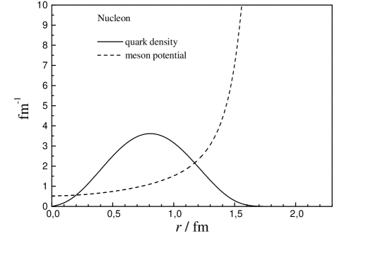
Figure 1: The baryon density (solid line) and the effective potentials (dashed line) generated by the self-consistently determined $\pi$, $\sigma$ and $\chi$ fields in the nucleon.

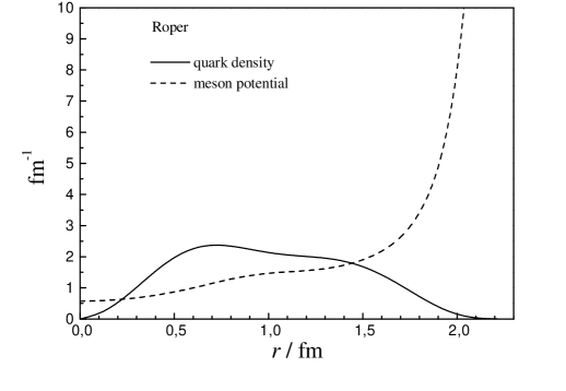
Figure 2: The baryon density (solid line) and the effective potentials (dashed line) generated by the self-consistently determined $\pi$, $\sigma$ and $\chi$ fields in the Roper.

4 Non-quark degrees of freedom

We have also investigated another possible type of excitation in which the quarks remain in the ground state configuration (1s)³ while the chromodielectric field and the $\sigma$-field oscillate. Such oscillations can be described by expanding the boson fields as small oscillations around their ground-state values. For the $\sigma$-field we write:

$$\hat{\sigma}(\vec{r})=\sum_{n}{1\over\sqrt{2\varepsilon_{n}}}\,\varphi_{n}(r){1\over\sqrt{4\pi}}\left[{\tilde{a}}_{n}+{\tilde{a}}^{\dagger}_{n}\right]+\sigma(r)\,,$$

where $\varphi_{n}$ and $\varepsilon_{n}$ satisfy the Klein-Gordon equation

$$\left(-\nabla^{2}+m^{2}+{{\rm d}^{2}{V}({\sigma}(r))\over{\rm d}{\sigma}(r)^{2}}\right)\varphi_{n}(r)=\varepsilon_{n}^{2}\varphi_{n}(r)\;.$$ (17)

A simple ansatz for the annihilation (creation) operator of the $n$-th mode is given by

$${\tilde{a}}_{n}=\int{\rm d}k\,\tilde{\varphi}_{n}(k)\left({\tilde{a}}(k)-\sqrt{2\pi\omega_{\sigma}(k)}\,\eta(k)\right)\;,\qquad{\tilde{a}}_{n}|N\rangle=0\;,$$ (18)

where $\eta(k)$ and $\tilde{\varphi}_{n}(k)$ are the Fourier transforms of $\sigma(r)$ and $\varphi_{n}(r)$, respectively, and $\omega_{\sigma}(k)=\sqrt{k^{2}+m_{\sigma}^{2}}$. The effective potential in (17) is given by

$$V_{\sigma\sigma}(r)=\lambda\left[C_{2}\phi(r)^{2}+3\sigma(r)(\sigma(r)+2\sigma_{v})\right]\,,$$ (19)

where $\sigma$ is the fluctuating part of the full field and $C_{2}$ is a projection coefficient slightly smaller than unity. Similar expressions hold for the $\chi$ field with the effective potential

$$V_{\chi\chi}(r)=-{3\over 2\pi}\,{g\over\chi(r)^{3}}\left[(\sigma(r)+\sigma_{v})(u(r)^{2}-v(r)^{2})+2\phi(r)u(r)v(r)\right]\,.$$ (20)

The effective potential turns out to be repulsive for the $\chi$-field and attractive for the $\sigma$-field; in the latter case there exists at least one bound state with the energy $\varepsilon_{1}$ of typically 100 MeV below the $\sigma$-meson mass.

The ansatz for the Roper can now be simply extended as

$$|{\rm{R}}^{*}\rangle=c_{1}|{\rm{R}}\rangle+c_{2}{\tilde{a}^{\dagger}}_{\sigma}|{\rm N}\rangle\;,$$ (21)

where $\tilde{a}^{\dagger}_{\sigma}$ is the creation operator for the lowest vibrational mode. The coefficients $c_{i}$ and the energy are determined by solving the generalized eigenvalue problem in the $2\times 2$ subspace. The solution with the lowest energy corresponds to the Roper, while the orthogonal combination to one of the higher excited states with nucleon quantum numbers, e.g., the ${\rm N}(1710)$, provided the $\sigma$-meson mass is sufficiently small. The energy of the Roper is reduced (see Table 1), though the effect is small due to weak coupling between the state (16) and the lowest vibrational state with the energy $\varepsilon_{1}$. The reduction becomes more important if the mass of the $\sigma$-meson is decreased. The energy of the combination orthogonal to the ground state is close to $E_{\mathrm{N}}+\varepsilon_{1}$ with $\sigma$-meson vibrational mode as the dominant component.

$m_{\sigma}$	$\ \ \ \ E_{\mathrm{N}}$	2s–1s	$\Delta E_{\mathrm{R}}$	$\Delta E_{\mathrm{R*}}$	$c_{2}$	$\ \ \ \ \ \ \varepsilon_{1}$
1200	1269	446	354	353	0.05	1090
700	1249	477	367	364	0.12	590

Table 1: For two $\sigma$-masses we show the nucleon energy ($E_{\mathrm{N}}$), the Roper-nucleon energy splittings calculated from the single particle energy difference (2s–1s), the state (16) ($\Delta E_{\mathrm{R}}$) and the state (21) ($\Delta E_{\mathrm{R*}}$). All energies are given in MeV.

5 Nucleon–Roper electromagnetic transitions

The electromagnetic nucleon-Roper transition amplitudes as well as the transition amplitudes to higher excitations with nucleon quantum numbers represent an important test which may help distinguish between the models listed at the beginning. The transverse helicity amplitude is defined as

$$A_{1/2}=-{\zeta}\,\sqrt{2\pi\alpha\over k_{W}}\int{\rm d}^{3}{{\kern-0.24994pt\hbox{\mbox{${r}$}}\kern-4.78937pt\kern 0.50003pt\hbox{\mbox{${r}$}}\kern-4.78937pt\kern-0.24994pt\raise 0.43304pt\hbox{\mbox{${r}$}}}}\,\ \langle\tilde{\rm{R}}_{+{1\over 2},M_{T}}|{{\kern-0.24994pt\hbox{\mbox{${J}$}}\kern-6.50694pt\kern 0.50003pt\hbox{\mbox{${J}$}}\kern-6.50694pt\kern-0.24994pt\raise 0.43304pt\hbox{\mbox{${J}$}}}}_{\rm em}({{\kern-0.24994pt\hbox{\mbox{${r}$}}\kern-4.78937pt\kern 0.50003pt\hbox{\mbox{${r}$}}\kern-4.78937pt\kern-0.24994pt\raise 0.43304pt\hbox{\mbox{${r}$}}}})\cdot{{\kern-0.24994pt\hbox{\mbox{${\epsilon}$}}\kern-4.05904pt\kern 0.50003pt\hbox{\mbox{${\epsilon}$}}\kern-4.05904pt\kern-0.24994pt\raise 0.43304pt\hbox{\mbox{${\epsilon}$}}}}_{+1}\,{\rm e}^{{\rm i}{{\kern-0.17496pt\hbox{\mbox{\scriptsize${k}$}}\kern-3.86458pt\kern 0.35002pt\hbox{\mbox{\scriptsize${k}$}}\kern-3.86458pt\kern-0.17496pt\raise 0.30313pt\hbox{\mbox{\scriptsize${k}$}}}}\cdot{{\kern-0.17496pt\hbox{\mbox{\scriptsize${r}$}}\kern-3.35255pt\kern 0.35002pt\hbox{\mbox{\scriptsize${r}$}}\kern-3.35255pt\kern-0.17496pt\raise 0.30313pt\hbox{\mbox{\scriptsize${r}$}}}}}|\tilde{\rm{N}}_{-{1\over 2},M_{T}}\rangle$$ (22)

where $k_{W}$ is the photon momentum at the photon point, and the scalar helicity amplitude as

$$S_{1/2}={\zeta}\,\sqrt{2\pi\alpha\over k_{W}}\int{\rm d}{{\kern-0.24994pt\hbox{\mbox{${r}$}}\kern-4.78937pt\kern 0.50003pt\hbox{\mbox{${r}$}}\kern-4.78937pt\kern-0.24994pt\raise 0.43304pt\hbox{\mbox{${r}$}}}}\,\langle\tilde{\rm{R}}_{+{1\over 2},M_{T}}|{J}^{0}_{\rm em}({{\kern-0.24994pt\hbox{\mbox{${r}$}}\kern-4.78937pt\kern 0.50003pt\hbox{\mbox{${r}$}}\kern-4.78937pt\kern-0.24994pt\raise 0.43304pt\hbox{\mbox{${r}$}}}})\,\,{\rm e}^{{\rm i}{{\kern-0.17496pt\hbox{\mbox{\scriptsize${k}$}}\kern-3.86458pt\kern 0.35002pt\hbox{\mbox{\scriptsize${k}$}}\kern-3.86458pt\kern-0.17496pt\raise 0.30313pt\hbox{\mbox{\scriptsize${k}$}}}}\cdot{{\kern-0.17496pt\hbox{\mbox{\scriptsize${r}$}}\kern-3.35255pt\kern 0.35002pt\hbox{\mbox{\scriptsize${r}$}}\kern-3.35255pt\kern-0.17496pt\raise 0.30313pt\hbox{\mbox{\scriptsize${r}$}}}}}|\tilde{\rm{N}}_{+{1\over 2},M_{T}}\rangle\,.$$ (23)

Here ${J}^{\mu}_{\rm em}$ is the EM current derived from the Lagrangian density (1):

$${J}^{\mu}_{\rm em}=\sum_{i=1}^{3}{\overline{q}}_{i}\gamma^{\mu}(i)\left({1\over 6}+{1\over 2}\tau_{0}{(i)}\right){q}_{i}+\left(\vec{{\pi}}\times\partial^{\mu}\vec{{\pi}}\right)_{0}\;.$$ (24)

The amplitudes (22) and (23) contain a phase factor $\zeta$ determined by the sign of the decay amplitude into the nucleon and the pion.

The new term in (21) does not contribute to the nucleon-Roper transition amplitudes. Namely, for an arbitrary EM transition operator $\hat{O}$ involving only quarks and pions we can write $\langle N|\tilde{a}_{1}\hat{O}|N\rangle=\langle N|[\tilde{a}_{1},\hat{O}]|N\rangle=0,$ because of (18) and since the operators $\tilde{a}_{n}$ commute with $\hat{O}$. The amplitudes (22)–(23) obtained in the framework of the present calculation can be found in Ref. [19]. We found a relatively large discrepancy at the photon point which can be attributed to a too weak pion field in the model. Such small contribution was already noticed in the calculation of nucleon magnetic moments [23] and of the electroproduction of the $\Delta$ [25]. The pion contribution to the charged states only accounts for a few percent of the total amplitude.

Though the chromodielectric model gives only a qualitative picture of the lowest radially excited states of the nucleon and their electroproduction amplitudes, it yields some interesting features, in particular the possibility of $\sigma$-meson vibrations. Its main advantage over other approaches is that all properties, including the electro-magnetic amplitudes and the resonance decay, can be calculated from a single Lagrangian without additional assumptions. It also allows us to treat exactly the orthogonalization of states which is particularly important in the description of nucleon radial excitations.

This work was supported by FCT (POCTI/FEDER), Portugal, and by The Ministry of Science and Education of Slovenia. MF acknowledges a travel grant from Fundação Calouste Gulbenkian (Lisbon), which made possible his participation in Hadrons 2002. He also would like to thank the organizers for the fine hospitality he enjoyed in Bento Gonçalves.

References

- [1] L. D. Roper, Phys. Rev. Lett. 12 (1964) 340.
- [2] D. E. Groom et al. (Particle Data Group), Eur. Phys. J. C15 (2000) 1, and references therein.
- [3] C. Gerhardt, Z. Phys. C 4 (1980) 311.
- [4] B. Boden, G. Krösen, Research Program at CEBAF, Report of the 1986 Summer Study Group, V. Burkert (ed.), p. 121.
- [5] Z. Li, Phys. Rev. D 44 (1991) 2841,
- [6] Z. Li, V. Burkert, Z. Li, Phys. Rev. D 46 (1992) 70.
- [7] L. S. Kisslinger, Z. Li, Phys. Rev. D 51 (1995) R5986.
- [8] S. Capstick, P. R. Page, Phys. Rev. D 60 (1999) 111501.
- [9] G. L. Strobel, Int. J. Theor. Phys. 39 (2000) 115.
- [10] Fl. Stancu, P. Stassart, Phys. Rev. D 41 (1990) 916.
- [11] Z. Li, F. E. Close, Phys. Rev. D 42 (1990) 2207.
- [12] S. Capstick, Phys. Rev. D 46 (1992) 1965; Phys. Rev. D 46 (1992) 2864.
- [13] H. J. Weber, Phys. Rev. C 41 (1990) 2783.
- [14] S. Capstick, B. D. Keister, Phys. Rev. D 51 (1995) 3598.
- [15] F. Cardarelli, E. Pace, G. Salmè, S. Simula, Phys. Lett. B 397 (1997) 13.
- [16] F. Cano, P. González, Phys. Lett. B 431 (1998) 270.
- [17] U. Meyer, A. J. Buchmann, A. Faessler, Phys. Lett. B 408 (1997) 19.
- [18] Y. B. Dong, K. Shimizu, A. Faessler, A. J. Buchmann, Phys. Rev. C 60 (1999) 035203.
- [19] P. Alberto, M. Fiolhais, B. Golli, J. Marques, Phys. Lett. B 523 (2001) 273.
- [20] W. Broniowski, T. D. Cohen, M. K. Banerjee, Phys. Lett. B 187 (1987) 229.
- [21] T. Neuber, M. Fiolhais, K. Goeke, J. N. Urbano, Nucl. Phys. A 560 (1993) 909.
- [22] M. C. Birse, Prog. Part. Nucl. Phys. 25 (1990) 1.
- [23] A. Drago, M. Fiolhais, U. Tambini, Nucl. Phys. A 609 (1996) 488.
- [24] B. Golli and M. Rosina, Phys. Lett. B 165 (1985) 347; M. C. Birse, Phys. Rev. D 33(1986) 1934.
- [25] M. Fiolhais, B. Golli, S. Širca, Phys. Lett. B 373 (1996) 229 ; L. Amoreira, P. Alberto and M. Fiolhais, Phys. Rev. C 62 (2000) 045202.