Abstract

We show that the initial-state interactions from gluon exchange between the incoming quark and the target spectator system lead to leading-twist single-spin asymmetries in the Drell-Yan process $H_{1}H_{2}^{\uparrow}\to\ell^{+}\ell^{-}X$. The QCD initial-state interactions produce a $T-$odd spin-correlation $\vec{S}_{H_{2}}\cdot\vec{P}_{H_{1}}\times\vec{Q}$ between the target spin and the virtual photon production plane which is not power-law suppressed in the Drell-Yan scaling limit at large photon virtuality $Q^{2}$ at fixed $x_{F}$. The single-spin asymmetry which arises from the initial-state interactions is not related to the target or projectile transversity distribution $\delta q_{H}(x,Q).$ The origin of the single-spin asymmetry in $\pi p^{\uparrow}\to\ell^{+}\ell^{-}X$ is a phase difference between two amplitudes coupling the proton target with $J^{z}_{p}=\pm{1\over 2}$ to the same final-state, the same amplitudes which are necessary to produce a nonzero proton anomalous magnetic moment. The calculation requires the overlap of target light-front wavefunctions with different orbital angular momentum: $\Delta L^{z}=1;$ thus the SSA in the Drell-Yan reaction provides a direct measure of orbital angular momentum in the QCD bound state. The single-spin asymmetry predicted for the Drell-Yan process $\pi p^{\uparrow}\to\ell^{+}\ell^{-}X$ is similar to the single-spin asymmetries in deep inelastic semi-inclusive leptoproduction $\ell p^{\uparrow}\to\ell^{\prime}\pi X$ which arises from the final-state rescattering of the outgoing quark. The Bjorken-scaling single-spin asymmetries predicted for the Drell-Yan and leptoproduction processes highlight the importance of initial- and final-state interactions for QCD observables.

1 Introduction

Single-spin asymmetries in hadronic reactions provide a remarkable window to QCD mechanisms at the amplitude level. In general, single-spin asymmetries measure the correlation of the spin projection of a hadron with a production or scattering plane [1]. Such correlations are odd under time reversal, and thus they can arise in a time-reversal invariant theory only when there is a phase difference between different spin amplitudes. Specifically, a nonzero correlation of the proton spin normal to a production plane measures the phase difference between two amplitudes coupling the proton target with $J^{z}_{p}=\pm{1\over 2}$ to the same final-state. The calculation requires the overlap of target light-front wavefunctions with different orbital angular momentum: $\Delta L^{z}=1;$ thus a single-spin asymmetry (SSA) provides a direct measure of orbital angular momentum in the QCD bound state.

Consider the SSA produced in semi-inclusive deep inelastic scattering $\ell p^{\uparrow}\to\ell^{\prime}\pi X$. In the target rest frame, such a single target spin correlation corresponds to the $T$-odd triple product $\vec{S}_{p}\cdot\vec{p}_{\pi}\times\vec{q}.$ (The covariant form of this correlation is $\epsilon_{\mu\nu\sigma\tau}S^{\mu}_{p}p^{\nu}q^{\sigma}p^{\tau}_{\pi}.)$ Significant asymmetries $A_{UL}$ and $A_{UT}$ of this type have in fact been observed for targets polarized parallel to or transverse to the lepton beam direction [2, 3].

In a recent paper [4] we have shown that the QCD final-state interactions (gluon exchange) between the struck quark and the proton spectator system in semi-inclusive deep inelastic lepton scattering can produce single-spin asymmetries which survive in the Bjorken limit. Such effects are proportional to the matrix element of a higher-twist quark-quark-gluon correlator in the target hadron, and thus it has been assumed on dimensional grounds that any SSA arising from this source must be suppressed by a power of the momentum transfer $Q$ in the Bjorken limit. However, another momentum scale enters into the semi-inclusive process—the transverse momentum ${\vec{r}}_{\perp}={\vec{p_{\pi}}}_{\perp}-{\vec{q}}_{\perp}$ of the emitted pion relative to the photon direction, and we have shown that the power-law suppression due to the higher-twist quark-quark-gluon correlator takes the form of an inverse power of $r_{\perp}$ rather $Q.$ As shown in the Appendix, $r^{2}_{\perp}$ can be written in terms of the invariant momentum transfer squared $t$ from the proton to the spectator system and the Bjorken variable.

Corrections from spin-one gluon exchange in the initial- or final-state of QCD processes are not suppressed at high energies because the coupling is vector-like. Therefore, as a consequence of the gauge coupling of QCD, single-spin asymmetries in semi-inclusive deep inelastic scattering survive in the Bjorken limit of large $Q^{2}$ at fixed $x_{bj}$ and fixed $\vec{r}_{\perp}$. Recently it has been shown [5, 6] that the same type of final-state interaction is the origin of the leading-twist diffractive component in deep inelastic scattering, implying that the pomeron is not a universal property of the target proton’s wavefunction, and that it depends in detail on the deep inelastic scattering (DIS) process itself. Diffractive processes in DIS in turn lead to nuclear shadowing in the case of nuclear targets, showing that shadowing is not an intrinsic property of nuclear wavefunctions.

The final-state phases which we compute are analogous to the “Coulomb” phases to the hard subprocess which arises from gauge interactions between outgoing charge particles in QED [7]. More specifically, we require the difference between the gauge interaction phases for the $J^{z}_{p}=\pm{1\over 2}$ amplitudes. The phases depend on the spin because the outgoing particles interact at different impact separation corresponding to their different relative orbital angular momentum.

In our previous paper [4], we explicitly evaluated the SSA for electroproduction for a specific model of a spin-$\frac{1}{2}$  proton of mass $M$ with charged spin-$\frac{1}{2}$  and spin-0 constituents of mass $m$ and $\lambda$, respectively, as in the QCD-motivated quark-diquark model of a nucleon. The basic leptoproduction reaction is then $\gamma^{*}p\to q(qq)_{0}$. Our analysis predicts a nonzero SSA for the target spin normal to the photon to quark-jet $\vec{S}_{p}\cdot\vec{p}_{q}\times\vec{q}$ which can be determined by using a jet variable such as thrust to determine the current quark direction; i.e., we predict a SSA even without final-state jet hadronization. Our mechanism is thus distinct from a description of SSA based on transversity and phased fragmentation functions.

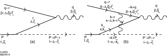
Figure 1: The initial-state interaction in the Drell-Yan process.

Recently Collins [8] has pointed out some important consequences of these results for SSA in deep inelastic scattering. In his treatment the final-state interactions of the struck quark are incorporated into Wilson line path-ordered exponentials which augment the light-cone wavefunctions. [See also [9].] Since the final-state interactions appear at short light-cone times $\Delta x^{+}={\cal O}(1/\nu)$ after the virtual photon acts, they can be distinguished from hadronization processes which occur over long times. Collins has stressed the fact that single-spin asymmetries probe the partonic structure associated with chiral-symmetry breaking. Furthermore, these results show that time-reversal-odd parton densities are allowed, opening up a whole range of phenomenological applications [10, 11, 12]. In particular, as noted by Collins, initial-state interactions between the annihilating antiquark and the spectator system of the target can produce single-spin asymmetries in the Drell-Yan process.

In this paper we shall extend our analysis to initial- and final-state QCD effects to predict single-spin asymmetries in hadron-induced hard QCD processes. Specifically, we shall consider the Drell-Yan (DY) type reactions [13] such as $\pi p^{\uparrow}\to\ell^{+}\ell^{-}X$. Here the target particle is polarized normal to the pion production plane. The target spin asymmetry can be produced due to the initial-state gluon-exchange interactions between the interacting antiquark coming from one hadronic system and the spectator system of the other. This is shown in the diagram of Fig. 1. The importance of initial-state interactions in the theory of massive lepton pair production, $Q_{\perp}$ broadening, and energy loss in a nuclear target has been discussed in Refs. [14, 15, 16].

The orientation of the target spin $S_{z}=\pm 1/2$ corresponds to amplitudes differing by relative orbital angular momentum $\Delta L^{z}=1.$ The initial-state interaction from a gluon exchanged between the annihilating antiquark and target spectator system depends in detail on this relative orbital angular momentum. In contrast, the initial or final-state interactions due to the exchange of gauge particles between partons not participating in the hard subprocess do not contribute to the SSA. Such spectator-spectator interactions occur at large impact separation and are not sensitive to just one unit difference $\Delta L^{z}=1$ of the orbital angular momentum of the target wavefunction.

Our mechanism thus depends on the interference of different amplitudes arising from the target hadron’s wavefunction and is distinct from probabilistic measures of the target such as transversity. It is also important to note that the target spin asymmetries which we compute in the DY and DIS processes require the same overlap of wavefunctions which enters the computation of the target nucleon’s magnetic moment. In addition, by selecting different initial mesons in the DY process, we can isolate the flavor of the annihilating quark and antiquark. The flavor dependence of single-spin asymmetries thus has the potential to provide detailed information of the spin and flavor content of nucleons at the amplitude level.

As in our analysis of semi-inclusive DIS, we shall calculate the single-spin asymmetry in the Drell-Yan process induced by initial-state interactions by adopting an effective theory of a spin-${1\over 2}$ proton of mass $M$ with charged spin-${1\over 2}$ and spin-$0$ constituents of mass $m$ and $\lambda$, respectively, as in a quark-diquark model. We will take the initial particle to be just an antiquark. The result for specific meson projectiles such as $Mp^{\uparrow}\to\ell^{+}\ell^{-}X$ is then obtained by convolution with the antiquark distribution of the incoming meson. One can also incorporate target nucleon wavefunctions with a quark-vector diquark structure. In a more complete study, one should allow for a many-parton light-front Fock state wavefunction representation of the target. The results, however, are always normalized to the quark contribution to the proton anomalous moment, and thus are basically model-independent.

2 Crossing

There is a simple diagrammatic connection between the amplitude describing the initial-state interaction of the annihilating antiquark, which gives a single-spin asymmetry for the Drell-Yan process $\pi p^{\uparrow}\to\ell^{+}\ell^{-}X$, and the final-state rescattering amplitude of the struck quark, which gives the single-spin asymmetries in semi-inclusive deep inelastic leptoproduction $\ell p^{\uparrow}\to\ell^{\prime}\pi X$. The crossing of the Feynman amplitude for $\gamma^{*}(\tilde{q})p(P)\to(\tilde{q}+r)(P-r)$ in DIS gives $(-\tilde{q}-r)p(P)\to\gamma^{*}(-\tilde{q})(P-r)$ for DY by reversing the four-vectors of the photon and quark lines. The outgoing quark with momentum $\tilde{q}+r$ in DIS becomes the incoming antiquark with momentum $-\tilde{q}-r$ in DY. We can use crossing of the Lorentz invariant amplitudes for DIS as a guide for obtaining the amplitudes for DY amplitude [17]. [In the next section it will be convenient to label $\tilde{q}=-q$ with $q^{+}>0.$ ]

In general, one cannot use crossing to relate imaginary parts of amplitudes to each other, since under crossing, real and imaginary parts become connected. However, in our case, the relevant one-gluon exchange diagrams in DIS and DY are both purely imaginary at high energy, so their magnitudes are related by crossing. Thus a crucial test of our mechanism is an exact relation between the magnitude and flavor dependence of the SSA in the Drell-Yan reaction and the SSA in deep inelastic scattering. We thus predict the DY SSA of the proton spin with the normal to the antiquark to virtual photon plane: $\vec{S}_{p}\cdot\vec{p}_{\overline{q}}\times\vec{\tilde{q}}$. It is identical – up to a sign – to the SSA computed in DIS for $\vec{S}_{p}\cdot\vec{p}_{q}\times\vec{q}$.

The phase arising from the initial- and final-state interactions in QCD is analogous to the Coulomb phase of Abelian QED amplitudes. The Coulomb phase depends on the product of charges and relative velocity of each ingoing and outgoing charged pair [7]. Thus the sign of the phase in DY and DIS are opposite because of the different color charge of the ingoing $\overline{3}_{C}$ antiquark in DY and the outgoing $3_{C}$ quark in DIS. In order to check the sign, we will carry out the DY calculation explicitly in the next section.

The asymmetry in the Drell-Yan process is thus the same as that obtained in DIS, with the appropriate identification of variables, but with the opposite sign. This has been stressed recently by Collins [8]. Therefore the single-spin asymmetry transverse to the production plane in the Drell-Yan process can be obtained from the results of our recent paper [4]:

$${\cal P}_{y} = -\ {e_{1}e_{2}\over 8\pi}\ {2\ \Bigl{(}\ \Delta\,M+m\ \Bigr{)}\ r^{1}\over\Big{[}\ \Bigl{(}\ \Delta\,M+m\ \Bigr{)}^{2}\ +\ {\vec{r}}_{\perp}^{2}\ \Big{]}}\ \Big{[}\ {\vec{r}}_{\perp}^{2}+\Delta(1-\Delta)(-M^{2}+{m^{2}\over\Delta}+{\lambda^{2}\over 1-\Delta})\ \Big{]}$$ (1)

$$\times \ {1\over{\vec{r}}_{\perp}^{2}}\ {\rm ln}{{\vec{r}}_{\perp}^{2}+\Delta(1-\Delta)(-M^{2}+{m^{2}\over\Delta}+{\lambda^{2}\over 1-\Delta})\over\Delta(1-\Delta)(-M^{2}+{m^{2}\over\Delta}+{\lambda^{2}\over 1-\Delta})}\ .$$

Here $\Delta={q^{2}\over 2P\cdot q}={q^{2}\over 2M\nu}$ where $\nu$ is the energy of the lepton pair in the target rest frame. The kinematics are given in detail in the Appendix.

3 Calculation

We can check the results of the previous section obtained using crossing by performing a direct calculation of the $\overline{q}p^{\uparrow}\to\gamma^{*}(qq)_{0}$ amplitude where we take a spin-zero diquark for the proton spectator system. The kinematics are $(q-r)p(P)\to\gamma^{*}(q)(P-r),$ as in Fig. 1. The $J^{z}=+{1\over 2}$ two-particle Fock state is given by [18, 19]

$$\left|\Psi^{\uparrow}_{\rm two\ particle}(P^{+},\vec{P}_{\perp}=\vec{0}_{\perp})\right>$$

$$= \int\frac{{\mathrm{d}}^{2}{\vec{k}}_{\perp}{\mathrm{d}}x}{{\sqrt{x(1-x)}}16\pi^{3}}\Big{[}\ \psi^{\uparrow}_{+\frac{1}{2}}(x,{\vec{k}}_{\perp})\,\left|+\frac{1}{2}\,;\,\,xP^{+}\,,\,\,{\vec{k}}_{\perp}\right>$$

$$\qquad+\psi^{\uparrow}_{-\frac{1}{2}}(x,{\vec{k}}_{\perp})\,\left|-\frac{1}{2}\,;\,\,xP^{+}\,,\,\,{\vec{k}}_{\perp}\right>\ \Big{]}\ ,$$

where

$$\left\{\begin{array}[]{l}\psi^{\uparrow}_{+\frac{1}{2}}(x,{\vec{k}}_{\perp})=(M+\frac{m}{x})\,\varphi\ ,\\ \psi^{\uparrow}_{-\frac{1}{2}}(x,{\vec{k}}_{\perp})=-\frac{(+k^{1}+{\mathrm{i}}k^{2})}{x}\,\varphi\ .\end{array}\right.$$ (3)

The scalar part of the wavefunction $\varphi$ depends on the dynamics. In the perturbative theory it is simply

$$\varphi=\varphi(x,{\vec{k}}_{\perp})=\frac{{e\over\sqrt{1-x}}}{M^{2}-{{\vec{k}}_{\perp}^{2}+m^{2}\over x}-{{\vec{k}}_{\perp}^{2}+\lambda^{2}\over 1-x}}\ .$$ (4)

In general one normalizes the Fock state to unit probability.

Similarly, the $J^{z}=-{1\over 2}$ two-particle Fock state has two components

$$\left\{\begin{array}[]{l}\psi^{\downarrow}_{+\frac{1}{2}}(x,{\vec{k}}_{\perp})=\frac{(+k^{1}-{\mathrm{i}}k^{2})}{x}\,\varphi\ ,\\ \psi^{\downarrow}_{-\frac{1}{2}}(x,{\vec{k}}_{\perp})=(M+\frac{m}{x})\,\varphi\ .\end{array}\right.$$ (5)

The spin-flip amplitudes in (3) and (5) have orbital angular momentum projection $l^{z}=+1$ and $-1$ respectively. The numerator structure of the wavefunctions is characteristic of the orbital angular momentum, and holds for both perturbative and non-perturbative couplings.

We require the interference between the tree amplitude of Fig. 1(a) and the one-loop amplitude of Fig. 1(b). The contributing amplitudes have the following structure through one-loop order:

$${\cal A}(\Uparrow\to\downarrow) = (M+{m\over\Delta})\ C\ (h+i{e_{1}e_{2}\over 8\pi}g_{1})$$ (6)

$${\cal A}(\Downarrow\to\downarrow) = \ ({+r^{1}-ir^{2}\over\Delta})\ \ C\ (h+i{e_{1}e_{2}\over 8\pi}g_{2})$$ (7)

$${\cal A}(\Uparrow\to\uparrow) = \ ({-r^{1}-ir^{2}\over\Delta})\ \ C\ (h+i{e_{1}e_{2}\over 8\pi}g_{2})$$ (8)

$${\cal A}(\Downarrow\to\uparrow) = (M+{m\over\Delta})\ C\ (h+i{e_{1}e_{2}\over 8\pi}g_{1})\ ,$$ (9)

where

$$C = -\ g\ e_{1}\ P^{+}\ {\sqrt{\beta-\Delta}}\ 2\ \Delta\ (1-\Delta)$$ (10)

$$h = {1\over{\vec{r}}_{\perp}^{2}+\Delta(1-\Delta)(-M^{2}+{m^{2}\over\Delta}+{\lambda^{2}\over 1-\Delta})}\ .$$ (11)

The label $\Uparrow/\Downarrow$ corresponds to $J^{z}_{p}=\pm{1\over 2}$ of the proton spin. The second label $\uparrow/\downarrow$ gives the spin projection $J^{z}_{q}=\pm{1\over 2}$ of the interacting spin-$\frac{1}{2}$  constituent antiquark of the other proton. Here $e_{1}$ and $e_{2}$ are the electric charges of the proton’s constituents $q$ and $(qq)_{0}$, respectively, and $g$ is the coupling constant of the effective proton-$q$-$(qq)_{0}$ vertex. The first term in (6) to (9) is the Born contribution of the tree graph. The crucial result will be the fact that the contributions $g_{1}$ and $g_{2}$ from the one-loop diagram Fig. 1(b) are different, and that their difference is infrared finite. A gauge boson mass $\lambda_{g}$ will be used as an infrared regulator in the calculation of $g_{1}$ and $g_{2}.$ The final result for $g_{1}-g_{2}$ is infrared finite, and $\lambda_{g}$ can be set to zero. The calculation will be done using light-cone time-ordered perturbation theory, or equivalently, by integrating Feynman loop-diagrams over $dk^{-}$.

We take $\vec{q}$ to lie in the $\hat{z}-\hat{x}$ plane, $\vec{q}=(q^{x},q^{y},q^{z})=(q^{1},0,q^{3})$. We denote $q^{+}$ as

$$q^{+}\ =\ \beta\ P^{+}\ .$$ (12)

From energy conservation, we get

$$q^{-}\ =\ {{\vec{q}}_{\perp}^{2}\over P^{+}\ (\ \beta-\Delta\ )}\ .$$ (13)

Then we have the relation

$$q^{2}\ =\ q^{+}q^{-}\ -\ {\vec{q}}_{\perp}^{2}\ =\ {\Delta\over\beta-\Delta}\ {\vec{q}}_{\perp}^{2}\ ,$$ (14)

where

$$\beta\ \geq\ \Delta\ .$$ (15)

Further details on the kinematics are given in the Appendix.

The covariant expression for the four one-loop amplitudes of diagram Fig. 1(b) is:

$${\cal A}^{\rm one-loop}(I)$$

$$= ig\ e_{1}\ (\ -e_{1}\ e_{2}\ )\ \int{d^{4}k\over(2\pi)^{4}}$$

$$\times{{\rm{\cal N}}(I)\over(k^{2}-m^{2}+i\epsilon)\ ((-k+q)^{2}-m^{2}+i\epsilon)((k-r)^{2}-\lambda_{g}^{2}+i\epsilon)((k-P)^{2}-\lambda^{2}+i\epsilon)}$$

$$= -ig\ e_{1}\ (\ -e_{1}\ e_{2}\ )\ \int{d^{2}{\vec{k}}_{\perp}\over 2(2\pi)^{4}}\int P^{+}dx\ {{\rm{\cal N}}(I)\over P^{+4}\ x\ (\beta-x)\ (x-\Delta)\ (1-x)}\$$

$$\times\int dk^{-}{1\over\left(k^{-}-{(m^{2}+{\vec{k}}_{\perp}^{2})-i\epsilon\over xP^{+}}\right)\left((-k^{-}+q^{-})-{(m^{2}+(-{\vec{k}}_{\perp}+{\vec{q}}_{\perp})^{2})-i\epsilon\over(\beta-x)P^{+}}\right)}$$

$$\times{1\over\left((k^{-}-r^{-})-{(\lambda_{g}^{2}+({\vec{k}}_{\perp}-{\vec{r}}_{\perp})^{2})-i\epsilon\over(x-\Delta)P^{+}}\right)\left((k^{-}-P^{-})+{(\lambda^{2}+{\vec{k}}_{\perp}^{2})-i\epsilon\over(1-x)P^{+}}\right)},\$$

where we used $k^{+}=xP^{+}.$ The numerators ${\rm{\cal N}}(I)$ are given by

$${\rm{\cal N}}(\Uparrow\to\downarrow) = N\ \ (M+{m\over x})$$ (17)

$${\rm{\cal N}}(\Downarrow\to\downarrow) = N\ \ ({+k^{1}-ik^{2}\over x})$$ (18)

$${\rm{\cal N}}(\Uparrow\to\uparrow) = N\ \ ({-k^{1}-ik^{2}\over x})$$ (19)

$${\rm{\cal N}}(\Downarrow\to\uparrow) = N\ \ (M+{m\over x})\ ,$$ (20)

where

$$N\ =\ 2P^{+}{\sqrt{\beta-\Delta}}\ \ x\ \,q^{-}\ \Bigl{(}-P^{+}[(1-x)+(1-\Delta)]\Bigr{)}\ ,$$ (21)

and $q^{-}={{\vec{q}}_{\perp}^{2}\over P^{+}(\beta-\Delta)}\$ as given in (13). For the [current]-[gauge boson propagator]-[current] factor, in Feynman gauge only the $-g^{+-}$ term of the gauge boson propagator $-g^{\mu\nu}$ contributes in the Bjorken limit, and it provides a factor proportional to $q^{-}$ in the numerator which cancels the $q^{-}$ in the denominator which provides the imaginary part. Therefore the result scales in the Bjorken limit.

The integration over $k^{-}$ in (3) does not give zero only if $0<x<1$. We first consider the region $\Delta<x<1$.

$${\cal A}^{\rm one-loop}(I)$$

$$= -ig\ e_{1}\ (\ -e_{1}\ e_{2}\ )\ \times\ (2\pi i)\ \int{d^{2}{\vec{k}}_{\perp}\over 2(2\pi)^{4}}\int P^{+}dx\ {{\rm{\cal N}}(I)\over P^{+4}\ x\ (\beta-x)\ (x-\Delta)\ (1-x)}\$$

$$\times{1\over\left(P^{-}-{(\lambda^{2}+{\vec{k}}_{\perp}^{2})-i\epsilon\over(1-x)P^{+}}-{(m^{2}+{\vec{k}}_{\perp}^{2})-i\epsilon\over xP^{+}}\right)\left(-P^{-}+{(\lambda^{2}+{\vec{k}}_{\perp}^{2})-i\epsilon\over(1-x)P^{+}}+q^{-}-{(m^{2}+(-{\vec{k}}_{\perp}+{\vec{q}}_{\perp})^{2})-i\epsilon\over(\beta-x)P^{+}}\right)}$$

$$\times{1\over\left(P^{-}-{(\lambda^{2}+{\vec{k}}_{\perp}^{2})-i\epsilon\over(1-x)P^{+}}-r^{-}-{(\lambda_{g}^{2}+({\vec{k}}_{\perp}-{\vec{r}}_{\perp})^{2})-i\epsilon\over(x-\Delta)P^{+}}\right)},\$$

where we used $k^{+}=xP^{+}$. The result is identical to that obtained from light-cone time-ordered perturbation theory.

The phases $\chi_{i}$ needed for single-spin asymmetries come from the imaginary part of (3), which arises from the potentially real intermediate state allowed before the rescattering. The imaginary part of the propagator (light-cone energy denominator) gives

$$-i\pi \delta \left(-P^{-}+{(\lambda^{2}+{\vec{k}}_{\perp}^{2})\over(1-x)P^{+}}+q^{-}-{(m^{2}+(-{\vec{k}}_{\perp}+{\vec{q}}_{\perp})^{2})\over(\beta-x)P^{+}}\right)$$ (23)

$$= \ -i\pi\ {1\over P^{+}}\ {(\beta-\Delta)^{2}\over{\vec{q}}_{\perp}^{2}}\ \delta(x\ -\ \Delta\ -\ {\overline{\delta}})\ ,$$

where

$${\overline{\delta}}\ =\ 2\ (\beta-\Delta)\ {{\vec{q}}_{\perp}\cdot({\vec{k}}_{\perp}-{\vec{r}}_{\perp})\over{\vec{q}}_{\perp}^{2}}\ .$$ (24)

Since the exchanged momentum $\overline{\delta}P^{+}$ is small, the light-cone energy denominator corresponding to the gauge boson propagator is dominated by the $({\vec{k}}_{\perp}-{\vec{r}}_{\perp})^{2}+\lambda^{2}_{g}\over(x-\Delta)$ term. This gets multiplied by $(x-\Delta)$, so only $({\vec{k}}_{\perp}-{\vec{r}}_{\perp})^{2}+\lambda^{2}_{g}$ appears in the propagator, independent of whether the photon is absorbed or emitted. The contribution from the region $0<x<\Delta$ thus compliments the contribution from the region $\Delta<x<1$.

We can integrate (3) over the transverse momentum using a Feynman parametrization to obtain the one-loop terms in (6) to (9).

$$g_{1} = \ \int_{0}^{1}d\alpha\ {1\over\alpha(1-\alpha){\vec{r}}_{\perp}^{2}+\alpha\lambda_{g}^{2}+(1-\alpha)\Delta(1-\Delta)(-M^{2}+{m^{2}\over\Delta}+{\lambda^{2}\over 1-\Delta})}$$ (25)

$$g_{2} = \ \int_{0}^{1}d\alpha\ {\alpha\over\alpha(1-\alpha){\vec{r}}_{\perp}^{2}+\alpha\lambda_{g}^{2}+(1-\alpha)\Delta(1-\Delta)(-M^{2}+{m^{2}\over\Delta}+{\lambda^{2}\over 1-\Delta})}\ .$$ (26)

We define:

$${\cal P}_{z} = {\cal C}^{-1}\ \Bigl{(}\ {|A(\Uparrow\to\uparrow)|^{2}-|A(\Downarrow\to\uparrow)|^{2}+|A(\Uparrow\to\downarrow)|^{2}-|A(\Downarrow\to\downarrow)|^{2}}\ \Bigr{)}$$ (27)

$${\cal P}_{x} = {\cal C}^{-1}\ \Bigl{(}\ (\ A(\Uparrow\to\uparrow)^{*}A(\Downarrow\to\uparrow)\ +\ A(\Uparrow\to\uparrow)A(\Downarrow\to\uparrow)^{*}\ )$$

$$\ \ \ +\ (\ A(\Uparrow\to\downarrow)^{*}A(\Downarrow\to\downarrow)\ +\ A(\Uparrow\to\downarrow)A(\Downarrow\to\downarrow)^{*}\ )\ \Bigr{)}$$

$${\cal P}_{y} = {\cal C}^{-1}\ \Bigl{(}\ i\ (\ A(\Uparrow\to\uparrow)^{*}A(\Downarrow\to\uparrow)\ -\ A(\Uparrow\to\uparrow)A(\Downarrow\to\uparrow)^{*}\ )$$

$$\ \ \ +\ i\ (\ A(\Uparrow\to\downarrow)^{*}A(\Downarrow\to\downarrow)\ -\ A(\Uparrow\to\downarrow)A(\Downarrow\to\downarrow)^{*}\ )\ \Bigr{)}\ ,$$

where the normalization from the unpolarized cross section is

$${\cal C}=|A(\Uparrow\to\uparrow)|^{2}+|A(\Downarrow\to\uparrow)|^{2}+|A(\Uparrow\to\downarrow)|^{2}+|A(\Downarrow\to\downarrow)|^{2}\ .$$ (30)

We can assume for convenience that the initial-state interactions generate a phase when exponentiated, as in the Coulomb phase analysis of QED. The rescattering phases $e^{i\chi_{i}}$ $(i=1,2)$ with $\chi_{i}={\rm tan}^{-1}({e_{1}e_{2}\over 8\pi}{g_{i}\over h})$ are thus distinct for the spin-parallel and spin-antiparallel amplitudes. The difference in phase arises from the orbital angular momentum $k_{\perp}$ factor in the spin-flip amplitude, which after integration gives the extra factor of the Feynman parameter $\alpha$ in the numerator of $g_{2}$ compared to $g_{1}$, as we can see in (25) and (26). Notice that the phases $\chi_{i}$ are each infrared divergent for zero gauge boson mass $\lambda_{g}\to 0$, as is characteristic of Coulomb phases. However, the difference $\chi_{1}-\chi_{2}$ which contributes to the single-spin asymmetry is infrared finite. We have verified that the Feynman gauge result is also obtained in the light-cone gauge using the principal value prescription. The small numerator coupling of the light-cone gauge boson is compensated by the small value for the exchanged $l^{+}=\overline{\delta}P^{+}$ momentum.

The virtual photon and produced hadron define the production plane which we will take as the ${\hat{z}}-{\hat{x}}$ plane. From Eqs. (6)-(9) and (3), the azimuthal single-spin asymmetry transverse to the production plane is given by

$${\cal P}_{y} = -\ {e_{1}e_{2}\over 8\pi}\ {2\ \Bigl{(}\ \Delta\,M+m\ \Bigr{)}\ r^{1}\over\Big{[}\ \Bigl{(}\ \Delta\,M+m\ \Bigr{)}^{2}\ +\ {\vec{r}}_{\perp}^{2}\ \Big{]}}\ \Big{[}\ {\vec{r}}_{\perp}^{2}+\Delta(1-\Delta)(-M^{2}+{m^{2}\over\Delta}+{\lambda^{2}\over 1-\Delta})\ \Big{]}$$ (31)

$$\times \ {1\over{\vec{r}}_{\perp}^{2}}\ {\rm ln}{{\vec{r}}_{\perp}^{2}+\Delta(1-\Delta)(-M^{2}+{m^{2}\over\Delta}+{\lambda^{2}\over 1-\Delta})\over\Delta(1-\Delta)(-M^{2}+{m^{2}\over\Delta}+{\lambda^{2}\over 1-\Delta})}\ ,$$

in agreement with the crossing properties described in section 2. The linear factor of $r^{1}=r^{x}$ reflects the fact that the single-spin asymmetry is proportional to ${\vec{S}}_{p}\cdot\vec{q}\times\vec{r}$ since $\vec{q}\sim-\hat{z}|\vec{q}|$ and ${\vec{S}}_{p}=\pm\hat{y}.$ The kinematics are given in more detail in the Appendix. The prediction for ${\cal P}_{y}$ as a function of $\Delta$ and $r_{\perp}$ is identical but with opposite sign to that illustrated in Fig. 4 of Ref. [4].

Our analysis can be generalized to the corresponding calculation in QCD. The initial-state interaction from gluon exchange has the strength ${e_{1}e_{2}\over 4\pi}\to C_{F}\alpha_{s}(\mu^{2}).$ The scale of $\alpha_{s}$ in the ${\overline{MS}}$ scheme can be identified with the momentum transfer carried by the gluon $\mu^{2}=e^{-5/3}({\vec{k}}_{\perp}-{\vec{r}}_{\perp})^{2}$ [20]. The matrix elements coupling the proton to its constituents will have the same numerator structure as the perturbative model since they are determined by orbital angular momentum constraints. The strengths of the proton matrix elements can be normalized quark by quark according to their contributions to the target nucleon’s anomalous magnetic moment weighted by the quark charge squared. In QCD, $r_{\perp}$ is the magnitude of the momentum of the current quark jet relative to the virtual photon direction. Notice that for large $r_{\perp}$, ${\cal P}_{y}$ decreases as $\alpha_{s}(r^{2}_{\perp})x_{bj}Mr_{\perp}\ln r^{2}_{\perp}\over{r}_{\perp}^{2}$. The physical proton mass $M$ appears since it is present in the ratio of the $L^{z}=1$ and $L^{z}=0$ matrix elements. This form is expected to be essentially universal.

4 Summary

We have shown that the same physical mechanism which produces a leading-twist single-spin asymmetry in semi-inclusive DIS, also leads to a leading twist single-spin asymmetry in the Drell-Yan process. The initial-state interaction between the annihilating antiquark with the spectator of the target produces the required phase correlation. The equality in magnitude, but opposite sign, of the single-spin asymmetries in semi-inclusive DIS and the corresponding Drell-Yan processes is an important check of our mechanism.

It has been conventional to assume that the effects of initial- and final-state interactions are always power-law suppressed for hard processes in QCD. In fact, this is not in general correct, as can be seen from our analyses of leading-twist single-spin asymmetries in the Drell-Yan process and semi-inclusive deep inelastic scattering. The initial- and final-state interactions which survive in the scaling limit occur in light-cone time $\tau={\cal O}(1/Q)$ immediately before or after the hard subprocess. Other initial- and final-state interactions, such as those between the spectator of the incident hadron and the spectator of the target hadron in the DY process, take place over long time scales, and they only provide inconsequential unitary phase corrections to the process. This is in accord with our intuition that interactions which occur at distant times cannot affect the primary reaction.

A natural framework for the wavefunctions which appear in the SSA calculations is the light-front Fock expansion [21, 22]. In principle, the light-front wavefunctions for hadrons can be obtained by solving for the eigen-solutions of the light-front QCD Hamiltonian. Such wavefunctions are real and include all interactions up to a given light-front time. The final-state gluon-exchange corrections which provide the SSA for semi-inclusive DIS occurs immediately after the virtual photon strikes the active quark. Such interactions are not included in the light-front wavefunctions, just as Coulomb final-state interactions are not included in the Schrödinger bound state wavefunctions in QED. Collins [8] has argued that since the relevant rescattering interactions of the struck quark occur very close in light-cone time to the hard interaction, one can augment the light-front wavefunctions by a Wilson line factor which incorporates the effects of the final-state interactions in semi-inclusive DIS. However, such augmented wavefunctions are not universal and process independent; for example, in the case of the DY process, an incoming Wilson line of opposite phase must be used.

Our formalism can be adopted to single-spin asymmetries in more general hard inclusive reactions, such as $\overline{p}p^{\uparrow}\to\pi X,$ where the pion is detected at high transverse momentum [23, 24]. In such cases one must identify the hard quark-gluon subprocess and analyze a set of gluon exchange corrections which connect the spectators of the polarized hadron with the active quarks and gluons of the hard subprocess. An example of a final-state interaction which can cause a single asymmetry in $\overline{p}p^{\uparrow}\to\pi X$ is shown in Fig. 2. However, this type of final-state interaction cannot be readily identified as an augmented target wavefunction. It is also clear from our analyses that there are potentially important corrections to the hard quark propagator in hard exclusive subprocesses such as deeply virtual Compton scattering or exclusive meson electroproduction. These rescattering interactions of the propagating quark can provide new single-spin observables and will correct analyses based on the handbag approximation.

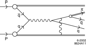
Figure 2: An example of a final-state interaction which can cause a single asymmetry in $\overline{p}p^{\uparrow}\to\pi X$.

It should be emphasized that the same overlap of light-front wavefunctions with $\Delta L^{z}=1$ which gives single-spin asymmetries also yields the Pauli form factor $F_{2}(t)$ and the generalized parton distribution $E(x,\zeta,t)$ entering deeply virtual Compton scattering [25, 26, 27, 28, 29]. Each quark of the target wavefunction appears additively, weighted linearly by the quark charge in the case of the Pauli form factor and weighted quadratically in the case of deep inelastic scattering, the Drell-Yan reaction and deeply virtual Compton scattering.

The empirical study of single-spin asymmetries in hard inclusive and exclusive processes thus provides a new window to the investigation of hadron spin, angular momentum, and flavor structure of hadrons.

Acknowledgments

We thank Harut Avakian, John Collins, Paul Hoyer, Xiang-dong Ji, and Stephane Peigne for helpful conversations.

Appendix: Kinematics

From Fig. 1 we have [$a=(a^{+},a^{-},{\vec{a}}_{\perp})$]

$$P = \Bigl{(}P^{+}\ ,\ {M^{2}\over P^{+}}\ ,\ {\vec{0}}_{\perp}\Bigr{)}$$ (32)

$$P^{\prime} = \Bigl{(}(1-\Delta)P^{+}\ ,\ {\lambda^{2}+{\vec{r}}_{\perp}^{2}\over(1-\Delta)P^{+}}\ ,\ -{\vec{r}}_{\perp}\Bigr{)}$$ (33)

$$q = \Bigl{(}\beta P^{+}\ ,\ {q^{2}+{\vec{q}}_{\perp}^{2}\over\beta P^{+}}\ ,\ {\vec{q}}_{\perp}\Bigr{)}$$ (34)

$$P_{\overline{q}} = \Bigl{(}(\beta-\Delta)P^{+}\ ,\ {m^{2}+({\vec{q}}_{\perp}-{\vec{r}}_{\perp})^{2}\over(\beta-\Delta)P^{+}}\ ,\ {\vec{q}}_{\perp}-{\vec{r}}_{\perp}\Bigr{)}\ ,$$ (35)

where

$$s-m^{2}-M^{2}=2P_{\overline{q}}\cdot P={m^{2}+({\vec{q}}_{\perp}-{\vec{r}}_{\perp})^{2}\over(\beta-\Delta)}+M^{2}(\beta-\Delta)\ .$$ (36)

Energy conservation gives

$${m^{2}+({\vec{q}}_{\perp}-{\vec{r}}_{\perp})^{2}\over(\beta-\Delta)}+{M^{2}}={q^{2}+{\vec{q}}_{\perp}^{2}\over\beta}+{\lambda^{2}+{\vec{r}}_{\perp}^{2}\over(1-\Delta)}\ .$$ (37)

Here $s$ and $q^{2}$ are large. It is convenient to work in a frame where $\beta-\Delta={\cal O}(1)$ and ${\vec{q}}_{\perp}^{2}$ is large so that $s\simeq{{\vec{q}}^{2}_{\perp}\over\beta-\Delta}.$ In such a frame, $\vec{q}\sim-\hat{z}|\vec{q}|.$ Then Eq. (37) gives

$${\vec{q}}_{\perp}^{2}={\beta-\Delta\over\Delta}q^{2}\ .$$ (38)

From (32), (34) and (38) we have

$$2P\cdot q={{\vec{q}}_{\perp}^{2}\over\beta-\Delta}+\beta M^{2}\ \simeq{q^{2}\over\Delta},$$ (39)

and thus to leading twist

$$\Delta\ =\ {q^{2}\over 2P\cdot q}\ ,$$ (40)

where $P\cdot q/M=\nu$ is the energy of the lepton pair in the target rest frame.

From (32) and (33) we have

$$2P\cdot P^{\prime}={\lambda^{2}+{\vec{r}}_{\perp}^{2}\over 1-\Delta}+(1-\Delta)M^{2}\ .$$ (41)

Since $t=(P-P^{\prime})^{2}$, we have $2P\cdot P^{\prime}=-t+M^{2}+\lambda^{2}$. Therefore, (41) gives

$${\vec{r}}_{\perp}^{2}\ =\ (1-\Delta)\Bigl{(}-t+M^{2}+\lambda^{2}-(1-\Delta)M^{2}\Bigr{)}-\lambda^{2}\ .$$ (42)

which relates ${\vec{r}}_{\perp}^{2}$ to invariants.

References

- [1] D. W. Sivers, Phys. Rev. D 43, 261 (1991).
- [2] HERMES Collaboration, A. Airapetian et al., Phys. Rev. Lett. 84, 4047 (2000); Phys. Rev. D 64, 097101 (2001).
- [3] A. Bravar, for the SMC Collaboration, Nucl. Phys. B (Proc. Suppl.) 79, 520 (1999).
- [4] S. J. Brodsky, D. S. Hwang and I. Schmidt, Phys. Lett. B 530, 99 (2002).
- [5] S. J. Brodsky, P. Hoyer, N. Marchal, S. Peigne and F. Sannino, hep-ph/0104291.
- [6] S. Peigne, hep-ph/0206138.
- [7] S. Weinberg, Phys. Rev. 140, B516 (1965).
- [8] J. C. Collins, Phys. Lett. B 536, 43 (2002).
- [9] X. d. Ji and F. Yuan, arXiv:hep-ph/0206057.
- [10] D. Boer and P. J. Mulders, Phys. Rev. D 57, 5780 (1998).
- [11] M. Anselmino and F. Murgia, Phys. Lett. B 442, 470 (1998).
- [12] D. Boer, Phys. Rev. D 60, 014012 (1999).
- [13] S. D. Drell and T. M. Yan, Phys. Rev. Lett. 25, 316 (1970) [Erratum-ibid. 25, 902 (1970)].
- [14] G. T. Bodwin, S. J. Brodsky and G. P. Lepage, Phys. Rev. Lett. 47, 1799 (1981).
- [15] G. T. Bodwin, S. J. Brodsky and G. P. Lepage, Phys. Rev. D 39, 3287 (1989).
- [16] S. J. Brodsky, A. Hebecker and E. Quack, Phys. Rev. D 55, 2584 (1997).
- [17] A. Brandenburg, V. V. Khoze and D. Muller, Phys. Lett. B 347, 413 (1995).
- [18] S. J. Brodsky and S. D. Drell, Phys. Rev. D 22, 2236 (1980).
- [19] S. J. Brodsky, D. S. Hwang, B. Q. Ma and I. Schmidt, Nucl. Phys. B 593, 311 (2001).
- [20] S. J. Brodsky, A. H. Hoang, J. H. Kühn and T. Teubner, Phys. Lett. B 359, 355 (1995).
- [21] G. P. Lepage and S. J. Brodsky, Phys. Rev. D 22, 2157 (1980).
- [22] S. J. Brodsky and G. P. Lepage, in: Perturbative Quantum Chromodynamics, edited by A. H. Mueller (World Scientific, Singapore 1989).
- [23] E704 Collaboration, A. Bravar et al., Phys. Rev. Lett. 77, 2626 (1996).
- [24] K. Heller, in Proceedings of Spin 96, C. W. de Jager, T. J. Ketel and P. Mulders, Eds., World Scientific (1997).
- [25] D. Muller, D. Robaschik, B. Geyer, F. M. Dittes and J. Horejsi, Fortsch. Phys. 42, 101 (1994).
- [26] X. D. Ji, Phys. Rev. Lett. 78, 610 (1997).
- [27] A. V. Radyushkin, Phys. Rev. D 56, 5524 (1997).
- [28] M. Diehl, T. Feldmann, R. Jakob and P. Kroll, Nucl. Phys. B 596, 33 (2001) [Erratum-ibid. B 605, 647 (2001)].
- [29] S. J. Brodsky, M. Diehl and D. S. Hwang, Nucl. Phys. B 596, 99 (2001).