Problems of QCD factorization in exclusive decays of $B$ meson to charmonium
Zhongzhi Song^(a) and Kuang-Ta Chao^(b,a)
(a) Department of Physics, Peking University, Beijing 100871, People’s Republic of China
(b) China Center of Advanced Science and Technology (World Laboratory), Beijing 100080, People’s Republic of China

Abstract

We study the exclusive decays of $B$ meson into P-wave charmonium states $\chi_{cJ}(J=0,1)$ in the QCD factorization approach with light-cone distribution functions describing the mesons in the processes. For $B\rightarrow\chi_{c1}K$ decay, we find that there are logarithmic divergences arising from nonfactorizable spectator interactions even at twist-2 order and the decay rate is too small to accommodate the experimental data. For $B\rightarrow\chi_{c0}K$ decay, we find that aside from the logarithmic divergences arising from spectator interactions at leading-twist order, more importantly, the factorization will break down due to the infrared divergence arising from nonfactorizable vertex corrections, which is independent of the specific form of the light-cone distribution functions. Our results may indicate that QCD factorization in the present form may not be safely applied to $B$-meson exclusive decays to charmonium states.
PACS numbers: 13.25.Hw; 14.40.Gx

Exclusive nonleptonic $B$-meson decays provide a important opportunity to determine the parameters of the Cabibbo-Kobayashi-Maskawa (CKM) matrix, to explore CP violation and to observe new physics effects. Recently, $B$ physics has received extensive experimental attention such as from high-energy experiments at the Tevatron and at the $e^{+}e^{-}~{}B$ factories. On the other hand, although the underlying weak decay of the $b$ quark is simple, quantitative understanding of nonleptonic $B$-meson decays is difficult due to the complicated strong-interaction effects.

Beneke et al. have considered two-body nonleptonic $B$-meson decays extensively including light-light as well as heavy-light final states within the QCD factorization approach[1, 2, 3]. The general idea is that in the heavy quark limit $m_{b}\gg\Lambda_{\mathrm{QCD}}$, the transition matrix elements of operators in the hadronic decay $B\to M_{1}M_{2}$ with $M_{1}$ being the recoiled meson and $M_{2}$ being the emitted meson can be calculated in an expansion in $1/m_{b}$ and $\alpha_{\mathrm{s}}$. The leading term in $1/m_{b}$ assumes a simple form[2]:

$$\langle M_{1}M_{2}|O_{i}|B\rangle\!=\!F^{BM_{1}}(m_{2}^{2})\int^{1}_{0}\!du\,T^{I}(u)\phi_{M_{2}}(u)\!+\!\int^{1}_{0}\!d\xi\,du\,dv\,T^{II}(\xi,u,v)\phi_{B}(\xi)\phi_{M_{1}}(v)\phi_{M_{2}}(u),$$ (1)

where $M_{2}$ is a light meson or a quarkonium and $F^{BM_{1}}$ is the $B\to M_{1}$ transition form factor; $\phi_{M}$ is meson light-cone distribution amplitude and $T^{I,II}$ are perturbatively calculable hard scattering kernels. If we neglect strong interaction corrections, eq.(1) reproduces the result of naive factorization. However, hard gluon exchange between $M_{2}$ and $BM_{1}$ system implies a nontrivial convolution of hard scattering kernels $T^{I,II}$ with the light-cone distribution amplitude $\phi_{M_{2}}$. This method works well for light-light final states[1, 3, 4, 5] as well as heavy-light final states[2, 6].

Exclusive $B$-meson decays to charmonium are important since those decays e.g. $B\to J/\psi K$ are regarded as the golden channels for the study of CP violation in $B$ decays. It is argued that because the size of the charmonium is small$(\sim 1/{\alpha_{\mathrm{s}}{m_{\psi}}})$ and its overlap with the $(B,K)$ system may be negligible[2], the same QCD factorization method as for $B\to\pi\pi$ can be used for $B\to J/\psi K(K^{*})$ decay. Indeed, explicit calculations[7, 8] show that the nonfactorizable vertex contribution is infrared safe and the spectator contribution is perturbatively calculable, where the light-cone distribution functions are used for $B$, $K$ as well as $J/\psi$ mesons. This small size argument for the applicability of QCD factorization for charmonia is intuitive and interesting, but it needs verifying for charmonium states e.g. the P-wave $\chi_{cJ}$ states other than the $J/\psi$. In addition, recently BaBar and Belle collaborations have measured the exclusive decays of $B\rightarrow\chi_{cJ}K(J=0,1)$[9, 10]. So, it is also interesting to compare the predictions based on the QCD factorization approach with the experimental data. In this letter, we report the problems of the QCD factorization approach encountered in these two decay channels. As in [7, 8], in the following we will use light-cone distribution functions to describe $B$, $K$, as well as charmonium mesons.

We first consider $\overline{B}\rightarrow\chi_{c1}K$ decay. The effective Hamiltonian is written as[11]

$$H_{\mathrm{eff}}=\frac{G_{F}}{\sqrt{2}}\Bigl{(}V_{cb}V_{cs}^{*}(C_{1}{\cal O}_{1}+C_{2}{\cal O}_{2})-V_{tb}V_{ts}^{*}\sum_{i=3}^{10}C_{i}{\cal O}_{i}\Bigr{)},$$ (2)

where $G_{F}$ is the Fermi constant, $C_{i}$ are the Wilson coefficients and $V_{q_{1}q_{2}}$ are the CKM matrix elements. Here the relevant operators ${\cal O}_{i}$ are given by

$$\,\,{\cal O}_{1}=(\overline{s}_{\alpha}b_{\beta})_{V-A}\cdot(\overline{c}_{\beta}c_{\alpha})_{V-A},\qquad\qquad\qquad~{}{\cal O}_{2}=(\overline{s}_{\alpha}b_{\alpha})_{V-A}\cdot(\overline{c}_{\beta}c_{\beta})_{V-A},$$

$${\cal O}_{3(5)}=(\overline{s}_{\alpha}b_{\alpha})_{V-A}\cdot\sum_{q}(\overline{q}_{\beta}q_{\beta})_{V-A(V+A)},\qquad~{}{\cal O}_{4(6)}=(\overline{s}_{\alpha}b_{\beta})_{V-A}\cdot\sum_{q}(\overline{q}_{\beta}q_{\alpha})_{V-A(V+A)},$$ (3)

$${\cal O}_{7(9)}={3\over 2}(\overline{s}_{\alpha}b_{\alpha})_{V-A}\cdot\sum_{q}e_{q}(\overline{q}_{\beta}q_{\beta})_{V+A(V-A)},~{}{\cal O}_{8(10)}={3\over 2}(\overline{s}_{\alpha}b_{\beta})_{V-A}\cdot\sum_{q}e_{q}(\overline{q}_{\beta}q_{\alpha})_{V+A(V-A)},$$

where $\alpha,~{}\beta$ are color indices and the sum over $q$ runs over $u,d,s,c$ and $b$. Here $(\bar{q}_{1}q_{2})_{V\pm A}=\bar{q}_{1}\gamma_{\mu}(1\pm\gamma_{5})q_{2}$.

To calculate the decay amplitude, we introduce the $\chi_{c1}$ decay constant $f_{\chi_{c1}}$ as[12]

$$\langle\chi_{c1}|\overline{c}(0)\gamma_{\mu}\gamma_{5}c(0)|0\rangle=-if_{\chi_{c1}}m_{\chi_{c1}}\epsilon^{*}_{\mu},\\$$ (4)

where $m_{\chi_{c1}}$ is the mass of $\chi_{c1}$ and $\epsilon$ is the $\chi_{c1}$ polarization vector. The decay constant $f_{\chi_{c1}}$ is a nonperturbative quantity and may be estimated from the potential models, the QCD sum rules, or lattice QCD calculations.

The leading-twist light-cone distribution amplitude of $\chi_{c1}$ can be expressed as

$$\langle\chi_{c1}(p,\epsilon)|\overline{c}_{\alpha}(y)c_{\beta}(z)|0\rangle=\frac{i}{4}\int_{0}^{1}du\cdot e^{i(up\cdot y+(1-u)p\cdot z)}f_{\chi_{c1}}m_{\chi_{c1}}\bigl{(}/{\epsilon}^{*}\gamma_{5}\bigr{)}_{\beta\alpha}\phi_{\chi_{c1}}(u),$$ (5)

where $u$ and $1-u$ are respectively the momentum fractions of the $c$ and $\bar{c}$ quarks inside the $\chi_{c1}$ meson, and the wave function $\phi_{\chi_{c1}}(u)$ for $\chi_{c1}$ meson is symmetric under $u\leftrightarrow 1-u$.

In naive factorization, we neglect the strong interaction corrections and the power corrections in $\Lambda_{\mathrm{QCD}}/m_{b}$. Then the decay amplitude at leading order is written as

$$iM_{0}=2if_{\chi_{c1}}m_{\chi_{c1}}\epsilon^{*}\cdot p_{B}F_{1}(m_{\chi_{c1}}^{2})\frac{G_{F}}{\sqrt{2}}\Bigl{[}V_{cb}V_{cs}^{*}(C_{2}+\frac{C_{1}}{N_{c}})-V_{tb}V_{ts}^{*}(C_{3}+\frac{C_{4}}{N_{c}}-C_{5}-\frac{C_{6}}{N_{c}})\Bigr{]},$$ (6)

where $p_{B}$ is the momentum of $B$ meson, $F_{1}$ is the $B\rightarrow K$ transition form factor and $N_{c}$ is the number of colors. We do not include the effects of the electroweak penguin operators since they are numerically small[11].

The form factors for $\overline{B}\rightarrow K$ are given as

$$\langle K(p_{K})|\overline{s}\gamma_{\mu}b|B(p_{B})\rangle=\Bigl{[}(p_{B}+p_{K})_{\mu}-\frac{m_{B}^{2}-m_{K}^{2}}{p^{2}}p_{\mu}\Bigr{]}F_{1}(p^{2})+\frac{m_{B}^{2}-m_{K}^{2}}{p^{2}}p_{\mu}F_{0}(p^{2}),$$ (7)

where $p=p_{B}-p_{K}$ is the momentum of $\chi_{c1}$ with $p^{2}=m_{\chi_{c1}}^{2}$, $m_{B}$ and $m_{K}$ are respectively the masses of $B$ and $K$ mesons. We will neglect the kaon mass for simplicity. We can use the ratio between these two form factors as[7]

$$\frac{F_{0}(p^{2})}{F_{1}(p^{2})}=1-\frac{p^{2}}{m_{B}^{2}}.$$ (8)

So we need only one of the two form factors to describe the decay amplitude.

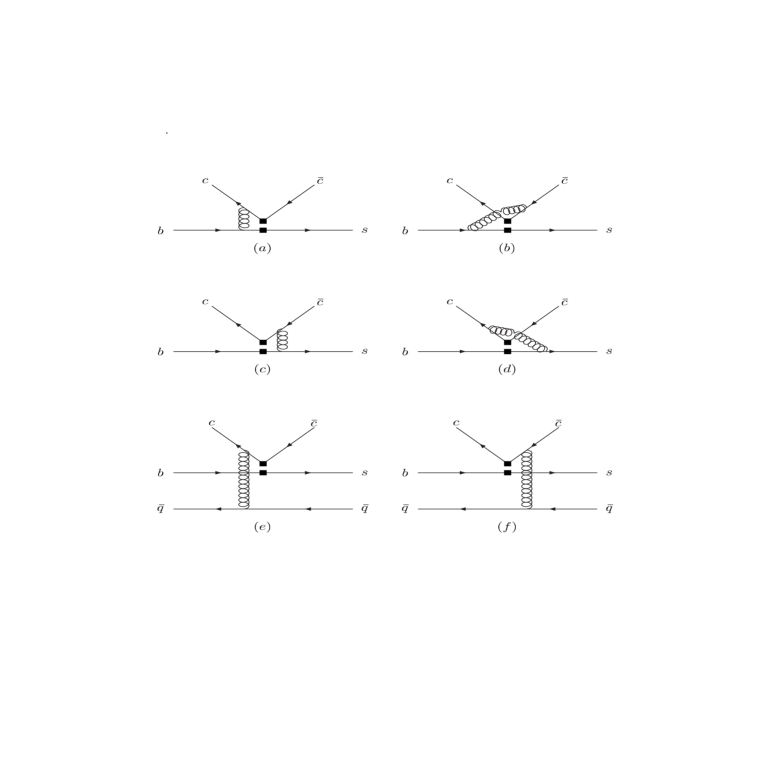
Figure 1: Feynman diagrams for vertex and spectator corrections to $\overline{B}\rightarrow\chi_{c1}K$.

Taking nonfactorizable corrections in Fig.1 into account, the full amplitude for $\overline{B}\rightarrow\chi_{c1}K$ in QCD factorization is written compactly as

$$iM=2if_{\chi_{c1}}m_{\chi_{c1}}\epsilon^{*}\cdot p_{B}F_{1}(m_{\chi_{c1}}^{2})\frac{G_{F}}{\sqrt{2}}\Bigl{[}V_{cb}V_{cs}^{*}a_{2}-V_{tb}V_{ts}^{*}(a_{3}-a_{5})\Bigr{]},$$ (9)

where the coefficients $a_{i}$ ($i=2,3,5$) in the naive dimension regularization(NDR) scheme are given by

$$a_{2}=C_{2}+\frac{C_{1}}{N_{c}}+\frac{\alpha_{s}}{4\pi}\frac{C_{F}}{N_{c}}C_{1}\Bigl{(}-18+12\ln\frac{m_{b}}{\mu}+f_{I}+f_{II}\Bigr{)},$$

$$a_{3}=C_{3}+\frac{C_{4}}{N_{c}}+\frac{\alpha_{s}}{4\pi}\frac{C_{F}}{N_{c}}C_{4}\Bigl{(}-18+12\ln\frac{m_{b}}{\mu}+f_{I}+f_{II}\Bigr{)},$$ (10)

$$a_{5}=C_{5}+\frac{C_{6}}{N_{c}}-\frac{\alpha_{s}}{4\pi}\frac{C_{F}}{N_{c}}C_{6}\Bigl{(}-6+12\ln\frac{m_{b}}{\mu}+f_{I}+f_{II}\Bigr{)},$$

where $C_{F}=(N_{c}^{2}-1)/(2N_{c})$ and $m_{b}$ is the $b$ quark mass.

The function $f_{I}$ is calculated from the four vertex correction diagrams (a, b, c, d) in Fig.1 and reads

$$f_{I}\!=\!\int_{0}^{1}du\phi_{\chi_{c1}}(u)\Bigl{[}\frac{3(1-2u)}{1-u}\ln u-3i\pi+3\ln(1-z)+\frac{z^{2}(1-u)^{2}\Bigl{(}\ln(1-z)-i\pi\Bigr{)}}{(1-zu)^{2}}$$

$$+\frac{2z(1-u)}{1-zu}+\Bigl{(}\frac{1-u}{(1-zu)^{2}}-\frac{u}{\bigl{(}1-z(1-u)\bigr{)}^{2}}\Bigr{)}z^{2}u\ln(zu)\Bigr{]},$$ (11)

where $z={m^{2}_{\chi_{c1}}}/{m^{2}_{B}}$, and we have already symmetrized the result with respect to $u\leftrightarrow 1-u$.

The function $f_{II}$ is calculated from the two spectator correction diagrams(e, f) in Fig.1 and it is given by

$$f_{II}=\frac{4\pi^{2}}{N_{c}}\frac{f_{K}f_{B}}{F_{1}(m_{\chi_{c1}}^{2})m_{B}^{2}}\frac{1}{1-z}\int_{0}^{1}d\xi\frac{\phi_{B}(\xi)}{\xi}\int_{0}^{1}dy\frac{\phi_{K}(y)}{y}\int_{0}^{1}du{\phi_{\chi_{c1}}(u)}[\frac{1}{u}+\frac{2z}{y(1-z)}],$$ (12)

where $\xi$ is the momentum fraction of the spectator quark in the $B$ meson and $y$ is the momentum fraction of the $s$ quark inside the $K$ meson, $\phi_{B}$, $\phi_{K}$ are the light-cone wave functions for the $B$ and $K$ meson respectively. $f_{II}$ corresponds to the $T^{II}$ term in Eq.(1).

The spectator contribution depends on the wave function $\phi_{B}$ through the integral

$$\int_{0}^{1}d\xi\frac{\phi_{B}(\xi)}{\xi}\equiv\frac{m_{B}}{\lambda_{B}}.$$ (13)

Since $\phi_{B}(\xi)$ is appreciable only for $\xi$ of order $\Lambda_{\mathrm{QCD}}/m_{B}$, $\lambda_{B}$ is of order $\Lambda_{\mathrm{QCD}}$. We will choose $\lambda_{B}\approx 300$ MeV in the numerical calculations[3].

There is an integral related to $\phi_{K}(y)$ in Eq.(12) which will give logarithmic divergence. Therefore QCD factorization breaks down even at leading order. This is different from $B\rightarrow J/\psi K$ decay which does not have logarithmic divergence at leading twist[7, 8]. The reason is that the logarithmic divergences arising from contributions of vector and tensor currents are cancelled out in the $B\rightarrow J/\psi K$ decay, whereas there is no such cancellation for the $B\rightarrow\chi_{c1}K$ decay. Following Ref.[3], we treat the divergent integral as an unknown parameter and write

$$\int_{0}^{1}dy\frac{\phi_{K}(y)}{y^{2}}=\int_{0}^{1}dy\frac{6(1-y)}{y}=6(X_{H}-1),$$ (14)

where the asymptotic form $\phi_{K}(y)=6y(1-y)$ is used for the kaon twist-2 light-cone distribution amplitude. And we will also choose $X_{H}=\ln(m_{B}/\Lambda_{QCD})$[3] as a rough estimate in our calculation.

For numerical analysis, we choose $F_{1}(m_{\chi_{c1}}^{2})=0.743$[13] and use the following input parameters:

$$m_{b}=4.8~{}\mbox{GeV},\ \ m_{B}=5.28~{}\mbox{GeV},\ m_{\chi_{c1}}=3.5~{}\mbox{GeV},$$

$$f_{\chi_{c1}}=230~{}\mbox{MeV},\ f_{B}=180~{}\mbox{MeV},\ f_{K}=160~{}\mbox{MeV}.$$ (15)

Here for the $\chi_{c1}$ decay constant $f_{\chi_{c1}}$ we give its expression in the heavy quarkonium potential model as

$$f_{\chi_{c1}}=\sqrt{\frac{18}{\pi m_{c}^{2}m_{\chi_{c1}}}}R^{\prime}(0),$$ (16)

where $R^{\prime}(0)$ is the derivative of the $\chi_{c1}$ radial wave function at the origin, and we may roughly estimate its value by using some potential models, e.g. given in Ref.[14].

	$C_{1}$	$C_{2}$	$C_{3}$	$C_{4}$	$C_{5}$	$C_{6}$
NDR	1.082	-0.185	0.014	-0.035	0.009	-0.041

Table 1: Next-to-leading-order Wilson coefficients in NDR scheme (See Ref.[11]) with $\mu=4.4$ GeV and $\Lambda^{(5)}_{\overline{\rm MS}}=225$ MeV.

$\phi_{\chi_{c1}}(u)$	$a_{2}$	$a_{3}$	$a_{5}$
$6u(1-u)$	0.1255-0.0815i	0.0040+0.0026i	-0.0027-0.0031i
$\delta(u-1/2)$	0.1154-0.0814i	0.0043+0.0026i	-0.0031-0.0031i

Table 2: The coefficients $a_{i}$ at $\mu=4.4$ GeV with different choices of $\phi_{\chi_{c1}}(u)$.

The specific form of the $\chi_{c1}$ light-cone distribution amplitude is not known, but as in the $J/\psi$ case (see [7, 8]) we may use the light meson asymptotic form $\phi_{\chi_{c1}}(u)=6u(1-u)$ as an approximate description. In the numerical analysis, we also consider the form $\phi_{\chi_{c1}}(u)=\delta(u-1/2)$, which comes from the naive expectation corresponding to the nonrelativistic limit of the distribution amplitude. Although there are uncertainties associated with the form of the distribution function, we will see shortly that the calculated decay rates are not sensitive to the choice of the distribution amplitude.

Using the next-to-leading-order (NLO) Wilson coefficients in Table. 1, we get the results of coefficients $a_{i}$ which are listed in Table. 2. With the help of these coefficients $a_{i}$, we calculate the decay branching ratios with two different choices of the $\chi_{c1}$ distribution amplitude and get

$${\mathrm{Br}}(\overline{B}\rightarrow\chi_{c1}K)=0.97\times 10^{-4},\,\,(\phi_{\chi_{c1}}(u)=6u(1-u));$$ (17)

$${\mathrm{Br}}(\overline{B}\rightarrow\chi_{c1}K)=0.87\times 10^{-4},\,\,(\phi_{\chi_{c1}}(u)=\delta(u-1/2)).$$ (18)

The measured branching ratio is[9]

$${\mathrm{Br}}(B^{0}\rightarrow\chi_{c1}K^{0})=(5.4\pm 1.4)\times 10^{-4},$$ (19)

which is about six times larger than the theoretical results.

We now consider the $B\rightarrow\chi_{c0}K$ decay. Unlike the $\chi_{c1}$ mode that we just analyzed, $\chi_{c0}$ does not have couplings to $V$ or $A$ currents, so this decay mode is prohibited in naive factorization. But it may occur if there is an exchange of an additional gluon[15, 16]. The branching ratio from experiment is[10]

$${\mathrm{Br}}(B^{+}\rightarrow\chi_{c0}K^{+})=(6.0\pm 2.1)\times 10^{-4}.$$ (20)

Similar to the calculation performed above, we write the $\chi_{c0}$ light-cone distribution amplitude in the following general form

$$\langle\chi_{c0}(p)|\overline{c}_{\alpha}(y)c_{\beta}(z)|0\rangle=\frac{i}{4}\int_{0}^{1}due^{i(up\cdot y+(1-u)p\cdot z)}\Bigl{[}f_{\chi_{c0}}^{s}m_{\chi_{c0}}\textsf{1}_{\beta\alpha}\phi_{\chi_{c0}}^{s}(u)+f_{\chi_{c0}}^{v}\bigl{(}/{p}\bigr{)}_{\beta\alpha}\phi_{\chi_{c0}}^{v}(u)\Bigr{]},$$ (21)

where $f_{\chi_{c0}}^{s},f_{\chi_{c0}}^{v},\phi_{\chi_{c0}}^{s}(u)$ and $\phi_{\chi_{c0}}^{v}(u)$ denote the $\chi_{c0}$ decay constants and light-cone distribution amplitudes, respectively for the scalar and vector currents. It is easy to see that for the scalar meson $\chi_{c0}$ the decay constants for the vector current and the antisymmetric tensor current all vanish (i.e., $\langle\chi_{c0}|\overline{c}\gamma_{\mu}c|0\rangle=\langle\chi_{c0}|\overline{c}\sigma_{\mu\nu}c|0\rangle=0$), and only the scalar current decay constant is nonzero. Therefore on the right hand side of Eq.(21) only the first term makes a real contribution and it is essentially the leading twist (twist-3) contribution. However, here we also list the second term (twist-2) in Eq.(21) in order to show that it would also give an infrared divergence contribution if the vector current decay constant were nonzero.

Because of charge conjugation invariance,$~{}\phi_{\chi_{c0}}^{s}(u)$ is symmetric while $~{}\phi_{\chi_{c0}}^{v}(u)$ is anti-symmetric under $u\leftrightarrow 1-u$. The Feynman diagrams of order $\alpha_{\mathrm{s}}$ correction for $B\rightarrow\chi_{c0}K$ are the same as those in Fig.1. In the calculation of $\chi_{c1}$, the contribution of the four vertex diagrams in Fig. 1 is infrared safe. However, we find there are infrared divergences arising from the vertex diagrams in the $B\rightarrow\chi_{c0}K$ decay. Keeping only the divergent terms, we get

$$V_{Div}=\frac{\alpha_{s}C_{F}}{\pi N_{c}}iF_{1}(m_{\chi_{c0}}^{2})\cdot\Bigl{\{}m_{c}m_{\chi_{c0}}f_{\chi_{c0}}^{s}\int_{0}^{1}\phi_{\chi_{c0}}^{s}(u)du\Bigl{[}-{1\over u}\ln{\lambda}\ln{z}\Bigr{]}+m_{B}^{2}f_{\chi_{c0}}^{v}\int_{0}^{1}\phi_{\chi_{c0}}^{v}(u)du$$

$$\times\Bigl{[}-\ln{\lambda}\ln{z}+(1-z)[\ln{\lambda}+{1\over 2}\ln^{2}(\frac{\lambda uz}{1-z})-i\pi\ln(\frac{\lambda uz}{1-z})]\Bigr{]}\Bigr{\}},$$ (22)

where $z=m_{\chi_{c0}}^{2}/m_{B}^{2}$ and $\lambda$ corresponds to the soft gluon momentum cutoff divided by the charm quark mass. The infrared divergence is explicitly seen as $\lambda\to 0$.

The contribution arising from spectator interactions is given by

$$H=\frac{\alpha_{s}C_{F}\pi}{N_{c}^{2}}if_{K}f_{B}\Bigl{[}\frac{m_{c}m_{\chi_{c0}}}{m_{B}^{2}-m_{\chi_{c0}}^{2}}f_{\chi_{c0}}^{s}\int_{0}^{1}d\xi\frac{\phi_{B}(\xi)}{\xi}\int_{0}^{1}dy\frac{\phi_{K}(y)}{{y}^{2}}\int_{0}^{1}du\frac{\phi_{\chi_{c0}}^{s}(u)}{u(1-u)}$$

$$+f_{\chi_{c0}}^{v}\int_{0}^{1}d\xi\frac{\phi_{B}(\xi)}{\xi}\int_{0}^{1}dy\frac{\phi_{K}(y)}{{y}}\int_{0}^{1}du\frac{\phi_{\chi_{c0}}^{v}(u)}{1-u}\Bigr{]}.$$ (23)

There are logarithmic divergences even in the leading-twist order. So, soft gluon exchange dominates $B\rightarrow\chi_{c0}K$ decay.

In the above calculations, we have chosen the heavy quark limit as $m_{b}\to\infty$ with $m_{c}/m_{b}$ fixed. In this limit, the logarithmic divergences in Eq.(12) for $B\rightarrow\chi_{c1}K$ decay, and the infrared divergences in Eq.(S0.Ex7) as well as the logarithmic divergences in Eq.(S0.Ex8) for $B\rightarrow\chi_{c0}K$ decay, will break down QCD factorization. Another choice of the heavy quark limit is that $m_{b}\to\infty$ with $m_{c}$ fixed. Then all the divergences mentioned above are power corrections and should be dropped out, so QCD factorization still holds in this limit. Physically, the latter case is equivalent to the limit of zero charm quark mass in which charmonium is regarded as a light meson. Obviously, the first choice of the heavy quark limit with $m_{c}/m_{b}$ fixed is more relevant in phenomenological analyses, and is also usually used in theoretical studies [2, 17], where it is expected that QCD factorization should apply to $B$ meson exclusive decays into charmonium in the limit $m_{c}\rightarrow\infty$ with corrections of order $\Lambda_{\rm QCD}/(m_{c}\alpha_{s})\sim 1$. Our result shows that this expectation holds for decays like $B\to J/\psi K$ but not for e.g. $B\to\chi_{c0}K$ where the vertex infrared divergence will break down factorization at order of $\Lambda_{\rm QCD}/(m_{c}\alpha_{s})$. It is also worthwhile to emphasize that the infrared divergences in Eq.(S0.Ex7) are more serious than the logarithmic divergences in Eqs.(12),(S0.Ex8). This is because, when one includes the parton transverse degrees of freedom, end-point singularities arising from spectator interactions can be regularized within the framework of $k_{T}$ factorization [18] and logarithmic divergences can then be removed. However, the infrared divergences due to nonfactorizable vertex corrections still exist, and they are independent of the specific form of the light-cone distribution functions.

In summary, we have studied the exclusive decays of $B$ meson into P-wave charmonium states $\chi_{cJ}(J=0,1)$ in the QCD factorization approach with light-cone distribution functions describing mesons involved in the processes. For $B\rightarrow\chi_{c1}K$ decay, the factorization breaks down due to logarithmic divergences arising from nonfactorizable spectator interactions at twist-2 order and the decay rate is too small to accommodate the data. The situation for $B\rightarrow\chi_{c0}K$ decay is even more serious because of the infrared divergence arising from nonfactorizable vertex corrections as well as logarithmic divergences due to spectator interactions at the leading-twist order. Considering the above problems encountered in $B\rightarrow\chi_{cJ}K$ decays and especially the infrared divergence in $B\rightarrow\chi_{c0}K$ decay, we intend to emphsize that the QCD factorization method with the present form may not be safely applied to exclusive decays of $B$ meson into charmonium, e.g. P-wave states. However, it should be noted that our results are obtained in QCD factorization by using the light-cone distribution functions for charmonium (as in e.g. refs.[7, 8]), which may not be a very appropriate description for heavy quarkonium. To further clarify the problem, many theoretical studies such as use of the nonrelativistic QCD for charmonium, the perturbative QCD factorization method, and the nonperturbative QCD effects should be attempted. In any case, a better understanding is definitely needed for describing $B$-meson exclusive decays to charmonium, and for reducing the big gap between the present theoretical results and the experimental observations.

References

• [1] M. Beneke et al., Phys. Rev. Lett. 83 (1999)1914.
• [2] M. Beneke et al., Nucl. Phys. B 591 (2000)313.
• [3] M. Beneke et al., Nucl. Phys. B 606 (2001)245.
• [4] T.Β Muta et al.,Phys.Β Rev.Β D 62 (2000)094020; D.S.Β Du, D.S.Β Yang and G.H.Β Zhu, Phys.Β Lett.Β B 488 (2000)46; D.S.Β Du et al., Phys.Β Rev.Β D 65 (2002)074001.
• [5] M.Z.Β Yang and Y.D.Β Yang, Phys.Β Rev.Β D 62 (2000)114019; H.Y.Β Cheng and K.C.Β Yang, Phys.Β Rev.Β D 64 (2001)074004; Phys.Β Lett.Β B 511 (2001)40.
• [6] J.Β Chay, Phys.Β Lett.Β B 476 (2000)339; M.Β Neubert and A.A.Β Petrov, Phys.Β Lett.Β B 519 (2001)50.
• [7] J. Chay and C. Kim, hep-ph/0009244.
• [8] H.Y.Β Cheng and K.C.Β Yang, Phys.Β Rev.Β D 63 (2001)074011;
H.Y.Β Cheng, Y.Y.Β Keum, and K.C.Β Yang, Phys.Β Rev.Β D 65 (2002)094023.
• [9] B. Aubert et al.(BaBar Collaboration), Phys. Rev. D 65 (2002)032001.
• [10] K. Abe et al.(Belle Collaboration), Phys. Rev. Lett. 88 (2002)031802.
• [11] G. Buchalla, A.J. Buras and M.E. Lautenbacher, Rev. Mod. Phys. 68 (1996)1125.
• [12] P. Ball, and V.M. Braun, Phys. Rev. D 54 (1996)2182.
• [13] P. Ball, JHEP 9809 (1998)005.
• [14] E.J. Eichten and C. Quigg, Phys. Rev. D 52 (1995)1726.
• [15] M. Beneke, F. Maltoni and I.Z. Rothstein, Phys. Rev. D 59 (1999)054003.
• [16] M.Β Diehl and G.Β Hiller, JHEP 0106 (2001)067.
• [17] M. Beneke, Nucl. Phys. Proc. Suppl. 111 (2002)62 (hep-ph/0202056).
• [18] J. Botts and G. Sterman, Nucl. Phys. B 225 (1989)62; H-n. Li and G. Sterman, Nucl. Phys. B 381 (1992)129.