A Duality as a Theory
for the Electroweak Interactions
Dissertation der Fakultät für Physik der
Ludwig-Maximilians-Universität München
vorgelegt von
Xavier Calmet
aus Marignane
Januar 2002

1. Gutachter: Prof. Dr. H. Fritzsch

2. Gutachter: Prof. Dr. J. Wess

Prüfungstag: 8.05.2002

Deutsche Zusammenfassung

Im Rahmen dieser Doktorarbeit wurde ein Modell für die elektroschwache Wechselwirkung entwickelt. Das Modell basiert auf der Tatsache, daß die sog. “Confinement”-Phase und Higgs-Phase der Theorie mit einem Higgs-Boson in der fundamentalen Darstellung der Eichgruppe $SU(2)$ identisch sind. In der Higgs-Phase wird die Eichsymmetrie durch den Higgsmechanismus gebrochen. Dies führt zu Massentermen für die Eichbosonen, und über die Yukawa-Kopplungen zu Massentermen für die Fermionen. In der “Confinement”-Phase ist die Eichsymmetrie ungebrochen. Nur $SU(2)$-Singuletts kann eine Masse zugeordnet werden, d.h., physikalische Teilchen müssen $SU(2)$-Singuletts sein. Man nimmt an, daß die rechtshändigen Quarks und Leptonen elementare Objekte sind, während die linkshändigen Dupletts Bindungszustände darstellen.

Es stellt sich heraus, daß das Modell in der “Confinement”-Phase dual zum Standard-Modell ist. Diese Dualität ermöglicht eine Berechnung des elektroschwachen Mischungswinkels und der Masse des Higgs-Bosons. Solange die Dualität gilt, erwartet man keine neue Physik.

Es ist aber vorstellbar, daß die Dualität bei einer kritischen Energie zusammenbricht. Diese Energieskala könnte sogar relativ niedrig sein. Insbesondere ist es möglich, daß das Standard-Modell im Yukawa-Sektor zusammenbricht. Falls die Natur durch die “Confinement”-Phase beschrieben wird, koennte man davon ausgehen, daß die leichten Fermionmassen erzeugt werden, ohne daß das Higgs-Boson an die Fermionen gekoppelt wird. Dann würde aber das Higgs-Boson anders als im Standard Modell zerfallen. Es ist jedoch auch vorstellbar, daß die Verletzung der Dualität erst bei hohen Energien stattfindet. Dann erwartet man neue Teilchen wie Anregungen mit Spin 2 der elektroschwachen Bosonen. Ebenso vorstellbar sind Fermionen-Substuktur-Effekte die beim anomal magnetischen Moment des Muons sichtbar werden.

Cette thèse est dediée à mes parents

Chapter 1 Introduction

During the past century, particle physics has undergone at least three revolutions.

The first of these revolutions happened when it was discovered by de Broglie [1] that particles have a dual character, sometimes they behave like solid entities sometimes like waves. In particular, it became clear that light is sometimes behaving like a stream of particles but, on the other hand, an electron is sometimes behaving like a wave. This led to the development of quantum mechanics.

Even more surprising was the second revolution. Particles can be created and annihilated. A particle and its antiparticle can be produced from the vacuum, and then they can annihilate. This had some profound consequences for quantum mechanics which had to be improved to take this fact into account. The mathematical tool which was developed to describe this phenomenon is called quantum field theory.

The third revolution was that the particles which were discovered could be classified according to simple schemes. The standard example is the eightfold way [2] proposed by Gell-Mann which allows to classify, according to a $SU(3)$ symmetry, all particles that interact strongly. Symmetries allow a much deeper understanding of the microscopic world. It was a big step between sampling particles and classifying them according to a symmetry. The $SU(3)$ symmetry allowed to predict particles that were not yet discovered and also allowed to understand that the strongly interacting particles that were observed could not be fundamental, but had to be bound states of some more fundamental fields, called quarks [2].

Another symmetry, Lorentz invariance, forced Dirac to introduce an antiparticle in his equation [3], and to posit the positron which was discovered shortly after. Actually it turns out that a relativistic quantum theory, for example Dirac’s equation, is inconsistent, and that the wave functions of relativistic quantum mechanics have to be replaced by quantum operators. This process is called the second-quantization, and it enables to describe processes where particles are created or destroyed. In that sense these revolutions are connected.

Symmetries in particle physics are symmetries of the action or in other words of the S-matrix. It became evident that any valid theory of particle physics should be Lorentz invariant or at least Lorentz invariant in a very good approximation. Thus all fields introduced in the action must fulfil the Klein-Gordon equation. The concept of Lorentz invariance introduces also the question of the discrete symmetries which are the charge conjugation $C$, the space reflection $P$ and the time reflection $T$. It turns out that if the fermions are quantized using anticommutation relations and bosons using commutation relations, then the S-matrix, or action, is invariant under the combination $CPT$.

Another concept which was discovered later is that of global and local gauge symmetries, i.e. the invariance of the action under certain global symmetries and local symmetries. Local gauge transformations are gauge transformations which are space-time dependent whereas global gauge transformations are independent on space-time. A gauge transformation is a transformation of the fields entering the action. Using Noether’s theorem, one can then deduce which quantities are conserved. For example in Quantum Electrodynamics (QED), there is a conserved quantity, the electric charge, corresponding to a $U(1)$ local gauge symmetry. The success of QED led Yang and Mills [4] to consider more complex non-Abelian gauge symmetries which eventually led to the standard model of particle physics.

Fundamental symmetries, like gauge symmetries or Lorentz symmetry, must be distinguished from approximate symmetries. For many technical issues it is often useful to consider symmetries that are exact in some limit, especially in Quantum Chromodynamics (QCD) where these approximatively valid symmetries are crucial to find relations between different non-perturbative quantities. An example of these symmetries is for example the isospin symmetry which is approximatively exact at low energy QCD.

After a century of great success applying symmetries in particle physics, it is still unclear why symmetries are so important in physics. We know that if we can identify one, it will have some very deep consequences, but there is still no primary principle which forces to require the action to be invariant under some given symmetry. We can only postulate a set of symmetries of the action, quantize and renormalize this action to obtain the Feynman rules and compute some observables to test whether a given symmetry is present or not in nature. There are two possibilities if a given symmetry is not observed, it can either be broken or it must be ruled out as a symmetry the theory.

In the present work we shall not try to understand why symmetries, and in particular gauge symmetries, are so crucial to particle physics. We shall take this as an given fact. Our main concern will rather be to try to understand how to break gauge symmetries. As we shall describe in this first chapter, the electroweak interactions are described by a broken $SU(2)\times U(1)$ local gauge symmetry. The main result of this work is that the electroweak interactions can be described as successfully by a confining theory, i.e. a theory based on an unbroken gauge symmetry, with a weak coupling constant. It turns out that this confining theory is dual to the standard model. This duality allows to find relations between some of the parameters of the standard electroweak model that are otherwise not present in the normal standard model with a broken electroweak symmetry. We shall first review the standard electroweak model, some of its problems and some of the solutions to these problems.

1.1 The standard electroweak model

In this section we shall discuss the standard model of the electroweak interactions. The weak interaction was first considered to be a local or point like interaction, the so-called Fermi interaction [5], before it was realized by Glashow [6], following the work of Schwinger [7], that a $SU(2)\times U(1)$ local gauge symmetry could account for this phenomenon and for Quantum Electrodynamics. But, if the electroweak gauge bosons were massless the electroweak interactions would be long range interactions. This is only partially the case, since QED is a long range interaction, but the weak interactions are short range. This implies that the gauge bosons are either confined and cannot propagate as free particles or that they are massive. The standard approach is to assume the latter. But, the $SU(2)\times U(1)$ gauge symmetry prohibits a mass term for the gauge bosons in the action. This led Weinberg and Salam [8] to assume that this symmetry is spontaneously broken and to apply the Higgs mechanism [9] to break this symmetry. It turns out that a theory with a gauge symmetry which is spontaneously broken remains renormalizable [10], and that this theory is thus consistent to any order in perturbation theory.

The standard model of the electroweak interactions is based on the gauge group $SU(2)_{L}\times U(1)_{Y}$, where the index $L$ stands for left and where $Y$ stands for hypercharge. In that model, parity is broken explicitly, left-handed fermions $\Psi^{a}_{L}=1/2(1-\gamma_{5})\Psi^{a}$ are transforming according to the fundamental representation of $SU(2)_{L}$ whereas right-handed fermions $\Psi^{a}_{R}=1/2(1+\gamma_{5})\Psi^{a}$ are singlets under this gauge group. The gauge boson of the $U(1)_{Y}$ gauge group is denoted by ${\cal A}_{\mu}$, and the three gauge bosons of the $SU(2)_{L}$ gauge group are called $B^{a}_{\mu}$, $a\in\{1,2,3\}$. The anti-symmetric tensors $f_{\mu\nu}$ and $F^{a}_{\mu\nu}$ are the field strength tensors of $U(1)_{Y}$ respectively $SU(2)_{L}$.

We start by writing down the Lagrangian of the standard electroweak model, taking into account only the first family of leptons ($L_{L},e_{r}$) and quarks ($Q_{L},u_{R},d_{R}$):

$${\cal L}_{h} = -\frac{1}{4}F^{a}_{\mu\nu}F^{a\mu\nu}-\frac{1}{4}f_{\mu\nu}f^{\mu\nu}+\bar{L}_{L}i\mathchoice{\ooalign{$\hfil\displaystyle\mkern 0.0mu/\hfil$\crcr$\displaystyle D$}}{\ooalign{$\hfil\textstyle\mkern 0.0mu/\hfil$\crcr$\textstyle D$}}{\ooalign{$\hfil\scriptstyle\mkern 0.0mu/\hfil$\crcr$\scriptstyle D$}}{\ooalign{$\hfil\scriptscriptstyle\mkern 0.0mu/\hfil$\crcr$\scriptscriptstyle D$}}L_{L}+\bar{Q}_{L}i\mathchoice{\ooalign{$\hfil\displaystyle\mkern 0.0mu/\hfil$\crcr$\displaystyle D$}}{\ooalign{$\hfil\textstyle\mkern 0.0mu/\hfil$\crcr$\textstyle D$}}{\ooalign{$\hfil\scriptstyle\mkern 0.0mu/\hfil$\crcr$\scriptstyle D$}}{\ooalign{$\hfil\scriptscriptstyle\mkern 0.0mu/\hfil$\crcr$\scriptscriptstyle D$}}Q_{L}+\bar{e}_{R}i\mathchoice{\ooalign{$\hfil\displaystyle\mkern 0.0mu/\hfil$\crcr$\displaystyle D$}}{\ooalign{$\hfil\textstyle\mkern 0.0mu/\hfil$\crcr$\textstyle D$}}{\ooalign{$\hfil\scriptstyle\mkern 0.0mu/\hfil$\crcr$\scriptstyle D$}}{\ooalign{$\hfil\scriptscriptstyle\mkern 0.0mu/\hfil$\crcr$\scriptscriptstyle D$}}e_{R}$$

$$+\bar{u}_{R}i\mathchoice{\ooalign{$\hfil\displaystyle\mkern 0.0mu/\hfil$\crcr$\displaystyle D$}}{\ooalign{$\hfil\textstyle\mkern 0.0mu/\hfil$\crcr$\textstyle D$}}{\ooalign{$\hfil\scriptstyle\mkern 0.0mu/\hfil$\crcr$\scriptstyle D$}}{\ooalign{$\hfil\scriptscriptstyle\mkern 0.0mu/\hfil$\crcr$\scriptscriptstyle D$}}u_{R}+\bar{d}_{R}i\mathchoice{\ooalign{$\hfil\displaystyle\mkern 0.0mu/\hfil$\crcr$\displaystyle D$}}{\ooalign{$\hfil\textstyle\mkern 0.0mu/\hfil$\crcr$\textstyle D$}}{\ooalign{$\hfil\scriptstyle\mkern 0.0mu/\hfil$\crcr$\scriptstyle D$}}{\ooalign{$\hfil\scriptscriptstyle\mkern 0.0mu/\hfil$\crcr$\scriptscriptstyle D$}}d_{R}-G_{e}\bar{e}_{R}({\bar{\phi}}L_{L})-G_{d}\bar{d}_{R}({\bar{\phi}}Q_{L})$$

$$-G_{u}\bar{u}_{R}({\phi}Q_{L})+h.c.+\frac{1}{2}(D_{\mu}\phi)^{\dagger}(D^{\mu}\phi)-\frac{\mu^{2}}{2}\phi^{\dagger}\phi-\frac{\lambda}{4}(\phi^{\dagger}\phi)^{2}.$$

The scalar doublet $\phi$ is the Higgs field and $\bar{\phi}=i\sigma_{2}\phi^{*}$. In the standard model this field enters the theory in the fundamental representation of the $SU(2)$ gauge group which has, as we shall see later, some nontrivial consequences. The quantum numbers of the fields entering the standard model Lagrangian are summarized in table 1.1. The covariant derivative is given by:

$$D_{\mu}=\partial_{\mu}-i\frac{g^{\prime}}{2}Y{\cal A}_{\mu}-i\frac{g}{2}\tau^{a}B^{a}_{\mu}.$$ (1.43)

The field strength tensors are as usual

$$F^{a}_{\mu\nu} = \partial_{\mu}B^{a}_{\nu}-\partial_{\nu}B^{a}_{\mu}+g\epsilon^{abc}B^{b}_{\mu}B^{c}_{\nu}$$ (1.44)

$$f_{\mu\nu} = \partial_{\mu}{\cal A}_{\nu}-\partial_{\nu}{\cal A}_{\mu}.$$ (1.45)

We have used the definitions:

$$L_{L}=\left(\begin{array}[]{c}\nu_{L}\\ e_{L}\end{array}\right),\ \ Q_{L}=\left(\begin{array}[]{c}u_{L}\\ d_{L}\end{array}\right),\ \ \phi=\left(\begin{array}[]{c}\phi^{0}\\ \phi^{-}\end{array}\right)\ \ \mbox{and}\ \ \bar{\phi}=i\sigma_{2}\phi^{*}=\left(\begin{array}[]{c}\phi^{+}\\ -{\phi^{0}}^{*}\end{array}\right).$$ (1.54)

	$SU(3)_{C}$	$SU(2)_{L}$	$U(1)_{Y}$	$U(1)_{Q}$
$L_{L}=\left(\begin{array}[]{c}\nu_{L}\\ e_{L}\end{array}\right)$	${\bf 1}$	${\bf 2}$	$-1$	$\left(\begin{array}[]{c}0\\ -1\end{array}\right)$
$e_{R}$	${\bf 1}$	${\bf 1}$	$-2$	$-1$
$Q_{L}=\left(\begin{array}[]{c}u_{L}\\ d_{L}\end{array}\right)$	${\bf 3}$	${\bf 2}$	$1/3$	$\left(\begin{array}[]{c}2/3\\ -1/3\end{array}\right)$
$u_{R}$	${\bf 3}$	${\bf 1}$	$4/3$	$2/3$
$d_{R}$	${\bf 3}$	${\bf 1}$	$-2/3$	$-1/3$
$\phi=\left(\begin{array}[]{c}\phi^{0}\\ \phi^{-}\end{array}\right)$	${\bf 1}$	${\bf 2}$	$-1$	$\left(\begin{array}[]{c}0\\ -1\end{array}\right)$
$B^{i}$	${\bf 1}$	${\bf 3}$	$0$	$(\pm 1,0)$
$A$	${\bf 1}$	${\bf 1}$	$0$	$0$
$G^{a}$	${\bf 8}$	${\bf 1}$	$0$	$0$

Table 1.1: The standard model fields, as usual the electric charge is given by the Gell-Mann-Nishijima relation $Q=\frac{1}{2}\left(\tau_{3}+Y\right)$. The fields $B^{i}$ with $i\in\{+,-,3\}$ denote the three electroweak gauge bosons and $A$ is the photon. The gluons $G^{i}$ are in the octet representation of $SU(3)_{C}$.

Obviously a mass term for the electroweak bosons of the form $m_{W}^{2}W^{i}_{\mu}W^{i\mu}$ would violate the gauge symmetry. In other words, the gauge invariance of the theory requires the gauge bosons to be massless. If the gauge bosons were massless, the electroweak interactions would be long range interactions. But, we know that the weak interactions are short range whereas QED is a long range interaction. Thus we have to break this symmetry partially.

1.1.1 The Higgs mechanism

The symmetry breaking scheme has already been introduced in the standard electroweak model Lagrangian. The Higgs mechanism [9] breaks the $SU(2)\times U(1)$ gauge symmetry spontaneously, which insures that the resulting theory is renormalizable. The potential of the Higgs boson is given by

$$V(\phi^{\dagger}\phi)=\frac{\mu^{2}}{2}\phi^{\dagger}\phi+\frac{\lambda}{4}(\phi^{\dagger}\phi)^{2}$$ (1.55)

The position of the minimum is dependent on the sign of the squared mass $\mu^{2}$ of the Higgs doublet. If it is positive, i.e. if the Higgs doublet squared mass has the right sign for the squared mass term of a scalar field, then the gauge symmetry is unbroken, and the minimum is at $\phi^{\dagger}\phi=0$. The Higgs mechanism postulates that the doublet is a tachyon, and thus requires $\mu^{2}<0$. In that case the potential has two extrema which are given by

$$\frac{dV(\rho)}{d\rho}=\mu^{2}\rho+\lambda\rho^{2}=\left(\mu^{2}+\lambda\rho\right)\rho=0$$ (1.56)

with $\rho^{2}=\phi^{\dagger}\phi$. The extrema are then

$$\rho_{1} = 0$$ (1.57)

$$\rho_{2} = \frac{-\mu^{2}}{\lambda}\equiv v^{2},$$ (1.58)

where $v$ is the so-called vacuum expectation value. The first solution is unstable and thus not the true vacuum of the theory. The standard procedure is to expand the Higgs field around its vacuum expectation value. It is convenient to fix the gauge, performing a $SU(2)$ rotation, at this stage. We shall choose the unitarity gauge

$$\phi = U_{2}\left(\matrix{\phi^{0}\cr\phi^{-}}\right)=\left(\matrix{\eta+v\cr 0}\right)$$ (1.59)

which allows to “rotate away” the Goldstone bosons. The Goldstone bosons are the three degrees of freedom which remain massless after spontaneous symmetry breaking. They are absorbed in the longitudinal degrees of freedom of the gauge bosons. The Higgs field is expanded around its vacuum expectation value $v$. This is a semi-classical approach. Of the four generators of $SU(2)\times U(1)$ three are broken by the Higgs mechanism. Only the linear combination $Q=1/2(\tau^{3}+Y)$ is left unbroken and thus leaves the vacuum invariant. This implies that a linear combination of the gauge fields of $SU(2)\times U(1)$ remains massless. It can be identified with the photon. Inserting the expansion of the Higgs field in the Lagrangian (1.1), one finds that the Higgs mechanism gives a mass to the electroweak bosons $W^{\pm}_{\mu}$ and $Z_{\mu}$, whereas the photon $A_{\mu}$ remains massless. The $Z_{\mu}$ and $A_{\mu}$ bosons are the mass eigenstates given by

$$A_{\mu} = \sin{\theta_{W}}W^{3}_{\mu}+\cos{\theta_{W}}{\cal A}_{\mu}$$

$$Z_{\mu} = \cos{\theta_{W}}W^{3}_{\mu}-\sin{\theta_{W}}{\cal A}_{\mu},$$ (1.60)

with

$$\cos{\theta_{W}}=\frac{g}{\sqrt{g^{2}+g^{\prime 2}}}\ \ \mbox{and}\ \ \sin{\theta_{W}}=\frac{g^{\prime}}{\sqrt{g^{2}+g^{\prime 2}}}.$$ (1.61)

The masses of the electroweak bosons are given by $m_{W^{\pm}}=gv/2$, $m_{Z}=\sqrt{g^{2}+{g^{\prime}}^{2}}v/2$ and $m_{A}=0$. It is important to notice that the mechanism responsible for the fermion mass generation is not the Higgs mechanism but rather the Yukawa mechanism. The Yukawa interactions generate a mass term for the fermions of the type

$$m_{e}=G_{e}v,\ \ \ m_{u}=G_{u}v,\ \ \mbox{and}\ \ \ m_{d}=G_{d}v.$$ (1.62)

There are thus two distinct mass generating mechanisms in the standard model.

Figure 1.1: Higgs potential before (continuous line) and after electroweak symmetry breaking (dotted line), the variable $\rho$ is defined by $\rho^{2}=\phi^{\dagger}\phi$.

1.1.2 Naturalness and Hierarchy problem

Albeit the standard model, which is the superposition of the standard electroweak model, described by $SU(2)_{L}\times U(1)_{Y}$, and of Quantum Chromodynamics, described by $SU(3)_{C}$, is extremely successful, it might not be the final theory of particle physics. The major objection is that it contains too many parameters that have to be measured and cannot be calculated from first principles. This led to a quest for the unification of the gauge interactions described by the three gauge groups $SU(3)$, $SU(2)$ and $U(1)$. There are two prime examples of such unification groups: $SU(5)$ [11] and $SO(10)$ [12]. In that framework the standard model is embedded in a larger gauge group whose gauge symmetry is broken at high energy called the grand unification scale (GUT) scale. The running of the coupling constant of the gauge group $SU(3)\times SU(2)\times U(1)$ suggests that the unification is taking place at a scale $\Lambda_{GUT}\approx 10^{16}$ to $10^{17}$ GeV depending on whether supersymmetry is present in Nature or not. The gauge hierarchy problem states that it is unnatural for the electroweak breaking scale $\Lambda_{EW}\approx 246$ GeV to be so small compared to the fundamental scale $\Lambda_{GUT}$.

A second potential problem with the standard model is that the Higgs boson is a scalar field. If a cutoff $\Lambda$ is used to renormalize the theory, the Higgs boson mass receives quadratic “corrections”

$$m_{H}^{2} \approx {m_{H}^{0}}^{2}+\frac{3g^{2}\Lambda^{2}}{32\pi^{2}m_{W}^{2}}\left(m^{2}_{H}+2m^{2}_{W}+m^{2}_{Z}-4\sum_{f}\left(\frac{n_{f}}{3}\right)m_{f}^{2}\right).$$ (1.63)

Nevertheless, this problem seems not very serious since the cutoff would not be apparent in a different renormalization scheme and secondly the standard model is a renormalizable theory. This means that all divergencies can be absorbed in the renormalized coupling constants and renormalized masses. Furthermore, it has been argued by Bardeen [13] that there is an approximate scale invariance symmetry of the perturbative expansion which protects the Higgs boson mass. The Higgs boson mass can be viewed as a soft breaking term for this symmetry. In that case fine tuning issues are related to nonperturbative aspects of the theory or embeddings of the standard model into a more complex theory.

The opinion of the author of this work is that none of these problems is very serious. The main problem of the standard model is that the symmetry breaking mechanism is implemented in a quite unnatural fashion. The Higgs boson which is introduced in the standard model is assumed to be a tachyon, i.e. its squared mass is adjusted to be negative at tree level. This might be a sign that a mechanism is required to trigger the Higgs mechanism.

There are many other motivations to extend the standard model. It is not clear yet which of these is the right one. In the following, we shall review a few typical models, which are all connected to solutions of these problems.

1.2 Extensions of the standard model

1.2.1 Composite models

In this section we shall review a composite model proposed around twenty years ago. The list of models proposed in the literature is very long. Three popular models were those proposed by Greenberg and Nelson [14], Fritzsch and Mandelbaum [15] and Abbott and Farhi [16]. For an extensive list of citations see [17] and [18]. The model Quantum Haplodynamics (QHD) we have chosen to review has been proposed by Fritzsch and Mandelbaum [15].

This model is inspired by QCD. In this approach, the weak interactions are residual effects due to the substructure of leptons, quarks and weak bosons. The constituents are called haplons, their quantum numbers are given in table 1.2.

	Color	Charge	Spin	H
$\alpha$	3	-1/2	1/2	+1 $n$
$\beta$	3	+1/2	1/2	+1 $n$
$x$	3	-1/6	0	-1 $\bar{n}$
$y$	$\bar{3}$	+1/2	0	-1 $\bar{n}$

Table 1.2: Quantum numbers of the haplons.

The haplons are assumed to be bound together by a very strong confining force, called hypercolor. The gauge group describing this interaction could be a $SU(N)$ gauge group (e.g. $SU(4)$) or a $U(1)$ gauge group. The spectrum of the model is as follows

$$u =(\bar{\alpha}\bar{x})_{3}\ \ \ \nu_{e} =(\bar{\alpha}\bar{y})_{1}$$ (1.64)

$$d =(\bar{\beta}\bar{x})_{3}\ \ \ e^{-} =(\bar{\beta}\bar{y})_{1}$$

$$W^{+} =(\bar{\alpha}\beta)\ \ \ W^{-} =(\bar{\beta}\alpha)$$

and two neutral bosons

$$W^{3}=\frac{1}{\sqrt{2}}(\bar{\alpha}\alpha-\bar{\beta}\beta)\ \ \ W^{0}=\frac{1}{\sqrt{2}}(\bar{\alpha}\alpha+\bar{\beta}\beta).$$

The neutral boson $W^{3}$, which mixes with the $U(1)$-photon, is identified with a component of the $Z$-boson. On the other side $W^{0}$ is assumed to be very heavy and not to contribute to the neutral currents. This model had the very pleasant feature of solving the gauge hierarchy problem and potentially the naturalness problem as in that case the weak interactions are not a gauge theory, but an effective theory with a cutoff at $\Lambda_{QHD}\approx 200$ GeV. Unfortunately the simplest version of this model is nowadays ruled out by experiments performed e.g. at LEP as are most of the composite models proposed long ago.

1.2.2 Technicolor

A more elaborate approach is that of technicolor theories. Again the literature is very rich, for reviews, see references [18] and [19].

We review the simplest possible (i.e. not extended) example of a technicolor theories [20, 21]. Technicolor theories are models where the electroweak symmetry breaking is due to dynamical effects.

Consider an $SU(N_{TC})$ gauge theory with fermions in the fundamental representation of the gauge group

$$\Psi_{L}=\left(\begin{array}[]{c}U\\ D\end{array}\right)_{L}\,\,\,\,\,\,\,\,U_{R},D_{R}~{}.$$ (1.67)

The fermion kinetic energy terms for this theory are

$${\cal L} = \bar{U}_{L}i\mathchoice{\ooalign{$\hfil\displaystyle\mkern 0.0mu/\hfil$\crcr$\displaystyle D$}}{\ooalign{$\hfil\textstyle\mkern 0.0mu/\hfil$\crcr$\textstyle D$}}{\ooalign{$\hfil\scriptstyle\mkern 0.0mu/\hfil$\crcr$\scriptstyle D$}}{\ooalign{$\hfil\scriptscriptstyle\mkern 0.0mu/\hfil$\crcr$\scriptscriptstyle D$}}U_{L}+\bar{U}_{R}i\mathchoice{\ooalign{$\hfil\displaystyle\mkern 0.0mu/\hfil$\crcr$\displaystyle D$}}{\ooalign{$\hfil\textstyle\mkern 0.0mu/\hfil$\crcr$\textstyle D$}}{\ooalign{$\hfil\scriptstyle\mkern 0.0mu/\hfil$\crcr$\scriptstyle D$}}{\ooalign{$\hfil\scriptscriptstyle\mkern 0.0mu/\hfil$\crcr$\scriptscriptstyle D$}}U_{R}+\bar{D}_{L}i\mathchoice{\ooalign{$\hfil\displaystyle\mkern 0.0mu/\hfil$\crcr$\displaystyle D$}}{\ooalign{$\hfil\textstyle\mkern 0.0mu/\hfil$\crcr$\textstyle D$}}{\ooalign{$\hfil\scriptstyle\mkern 0.0mu/\hfil$\crcr$\scriptstyle D$}}{\ooalign{$\hfil\scriptscriptstyle\mkern 0.0mu/\hfil$\crcr$\scriptscriptstyle D$}}D_{L}+\bar{D}_{R}i\mathchoice{\ooalign{$\hfil\displaystyle\mkern 0.0mu/\hfil$\crcr$\displaystyle D$}}{\ooalign{$\hfil\textstyle\mkern 0.0mu/\hfil$\crcr$\textstyle D$}}{\ooalign{$\hfil\scriptstyle\mkern 0.0mu/\hfil$\crcr$\scriptstyle D$}}{\ooalign{$\hfil\scriptscriptstyle\mkern 0.0mu/\hfil$\crcr$\scriptscriptstyle D$}}D_{R}~{},$$ (1.100)

and, like QCD in the $m_{u}$, $m_{d}\to 0$ limit, they exhibit a chiral $SU(2)_{L}\times SU(2)_{R}$ symmetry.

As in QCD, exchange of technigluons in the spin zero, isospin zero channel is attractive, causing the formation of a condensate

$${\lower 35.0pt\hbox{ \epsfbox{tndiag.ps}}\ \ \rightarrow\ \ \langle\bar{U}_{L}U_{R}\rangle=\langle\bar{D}_{L}D_{R}\rangle\neq 0\,,}$$ (1.101)

which dynamically breaks $SU(2)_{L}\times SU(2)_{R}\to SU(2)_{V}$. These broken chiral symmetries imply the existence of three massless Goldstone bosons, the analog of the pions in QCD.

Now we consider gauging $SU(2)_{W}\times U(1)_{Y}$ with the left-handed fermions transforming as weak doublets and the right-handed ones as weak singlets. To avoid gauge anomalies, in this one-doublet technicolor model, the left-handed technifermions are assumed to have hypercharge zero and the right-handed up- and down-technifermions to have hypercharge $\pm 1/2$. The spontaneous breaking of the chiral symmetry breaks the weak interactions down to electromagnetism. The would-be Goldstone bosons become the longitudinal components of the $W$ and $Z$

$$\pi^{\pm},\,\pi^{0}\,\rightarrow\,W^{\pm}_{L},\,Z_{L}~{},$$ (1.102)

which acquire a mass

$$M_{W}={gF_{TC}\over 2}~{}.$$ (1.103)

Here $F_{TC}$ is the analog of $f_{\pi}$ in QCD. In order to obtain the experimentally observed masses, we must have $F_{TC}\approx 246$ GeV and hence this model is essentially like QCD scaled up by a factor of

$${F_{TC}\over f_{\pi}}\approx 2500\,.$$ (1.104)

Since there are no fundamental scalars in the theory, there is not any unnatural adjustment required to absorb quadratic divergencies of scalar masses. The mass generation problem of the electroweak bosons can thus be solved in a very elegant fashion. The gauge hierarchy problem is solved in such a theory, because the scale of the electroweak symmetry breaking is a dynamical quantity which could eventually be calculated. Nevertheless there is a potentially serious problem with the mass generation of the fermions in such theories. The model we have presented does not yet have a mechanism to generate fermion masses.

The model has to be embedded in a more complex theory, so-called extended Technicolor theories (ETC) [22, 23]. In ETC models, technifermions couple to ordinary fermions. At energies low compared to the ETC gauge-boson mass, $M_{ETC}$, these effects can be treated as local four-fermion interactions

$${\lower 35.0pt\hbox{\epsfbox{etcdiag.ps}}}\ \ \rightarrow\ \ {{g_{ETC}^{2}\over M^{2}_{ETC}}}(\overline{\Psi}_{L}U_{R})({\overline{q}_{R}q_{L}})~{}.$$ (1.105)

After technicolor chiral-symmetry breaking and the formation of a $\langle\bar{U}U\rangle$ condensate, such an interaction gives rise to a mass for an ordinary fermion

$$m_{q}\approx{{g_{ETC}^{2}\over M^{2}_{ETC}}}\langle\overline{U}U\rangle_{ETC}~{},$$ (1.106)

where $\langle\overline{U}U\rangle_{ETC}$ is the value of the technifermion condensate evaluated at the ETC scale (of order $M_{ETC}$). The condensate renormalized at the ETC scale in eq. (1.106) can be related to the condensate renormalized at the technicolor scale as follows

$$\langle\overline{U}U\rangle_{ETC}=\langle\overline{U}U\rangle_{TC}\exp\left(\int_{\Lambda_{TC}}^{M_{ETC}}{d\mu\over\mu}\gamma_{m}(\mu)\right)~{},$$ (1.107)

where $\gamma_{m}(\mu)$ is the anomalous dimension of the fermion mass operator and $\Lambda_{TC}$ is the analog of $\Lambda_{QCD}$ for the technicolor interactions. One finds

$$\langle\overline{U}U\rangle_{ETC}\approx\langle\overline{U}U\rangle_{TC}\approx 4\pi F^{3}_{TC}~{},$$ (1.108)

using dimensional analysis. In this case eq. (1.106) implies that

$$\frac{M_{ETC}}{g_{ETC}}\approx 40\mbox{TeV}\left(\frac{F_{TC}}{250\ \mbox{GeV}}\right)^{3\over 2}\left(\frac{100\ \mbox{MeV}}{m_{q}}\right)^{1\over 2}~{}.$$ (1.109)

It is not easy to build technicolor models that give a mass to fermions while remaining simple. Besides this most of the ETC models predict large deviations from the standard model predictions, and in particular rare decays of the type $\mu\to e\gamma$ for which the experimental limits are quite restrictive. It is also difficult to understand how light fermion masses can be generated since

$$m_{q}\sim\frac{4\pi g_{ETC}^{2}}{M_{ETC}^{2}}F^{3}_{TC}.$$ (1.110)

This requires $M_{ETC}$ to be in the range of $100$ TeV for the $s$-quark or for the muon. But, $M_{ETC}=100$ TeV is too low to be invisible, e.g. in $\bar{K}K$ mixing.

Nevertheless an interesting proposition has been made recently. The case of mass generation for fermions in a simple technicolor theory has been reconsidered [24]. If the fermion global chiral symmetries are broken by the inclusion of four-fermion interactions, it is found that the system can be nonperturbatively unstable under fermion mass fluctuations driving the formation of an effective coupling between the technigoldstone bosons and the ordinary fermions. A minimization of an effective action for the corresponding composite operators leads to a dynamical generation of light fermion masses $\sim M\exp(-k/g^{2})$, where $M$ is some cutoff mass and where $k$ is a parameter which depends on the coupling constants of the four-fermion interactions.

Technicolor theories are still an acceptable alternative to the Higgs mechanism. A better understanding of the non-perturbative aspects of this theory might avoid to extend the plain technicolor models to ETC models which are getting very complicated and are thus not very elegant.

1.2.3 Supersymmetry

Low energy supersymmetry is a natural candidate to solve the naturalness problem of the Higgs boson mass (see [25] and [26] for reviews). Supersymmetry [27] is a symmetry between bosons and fermions, i.e. a symmetry between states of different spin. For example, a spin-0 particle is mapped to a spin-$\frac{1}{2}$ particle under a supersymmetry transformation. The particle states in a supersymmetric field theory form representations (supermultiplets) of the supersymmetry algebra. There is an equal number of bosonic degrees of freedom $n_{B}$ and fermionic degrees of freedom $n_{F}$ in a supermultiplet

$$n_{B}=n_{F}.$$ (1.111)

The masses of all states in a supermultiplet are degenerate. In particular the masses of bosons and fermions are equal

$$m_{B}=m_{F}.$$ (1.112)

We shall illustrate how supersymmetry can solve the naturalness problem. Consider the following (non-supersymmetric) Lagrangian of a complex scalar $A$ and a Weyl fermion $\chi$

$${\cal L}= - \partial_{\mu}\bar{A}\partial^{\mu}A-i\bar{\chi}\bar{\sigma}^{\mu}\partial_{\mu}\chi-\frac{1}{2}\,m_{f}\,(\chi\chi+\bar{\chi}\bar{\chi})-m^{2}_{b}\,\bar{A}A$$ (1.113)

$$- \;Y\,(A\chi\chi+\bar{A}\bar{\chi}\bar{\chi})\;-\;\lambda\,(\bar{A}A)^{2}\ .$$

This Lagrangian is supersymmetric if $m_{f}=m_{b}$ and $Y^{2}=\lambda$, but let us not consider this choice of parameters at first. ${\cal L}$ has a chiral symmetry for $m_{f}=0$ given by

$$A\rightarrow e^{-2i\alpha}\,A\ ,\qquad\chi\rightarrow e^{i\alpha}\,\chi\ .$$ (1.114)

This symmetry prohibits the generation of a fermion mass by quantum corrections. For $m_{f}\neq 0$ the fermion mass does receive radiative corrections, but all possible diagrams have to contain a mass insertion as can be seen from the one-loop diagram shown in figure 1.2. Since the propagator of the boson (upper dashed line in the diagram) is $\sim\frac{1}{k^{2}}$ while the propagator of the fermion (lower solid line) is $\sim\frac{1}{k}$ one obtains a mass correction which is proportional to $m_{f}$

Figure 1.2: One loop corrections to the fermion mass and to the boson mass.

$$\delta m_{f}\sim Y^{2}m_{f}\ln{\frac{m_{f}^{2}}{\Lambda^{2}}}\ ,$$ (1.115)

where $\Lambda$ is the ultraviolet cutoff. Hence the mass of a chiral fermion does not receive large radiative corrections if the bare mass is small.

The diagrams giving the one-loop corrections to $m_{b}$ are shown in figure 1.2. Both diagrams are quadratically divergent but they have an opposite sign because in the second diagram fermions are running in the loop. One finds

$$\delta m_{b}^{2}\sim(\lambda-~{}Y^{2})\,\Lambda^{2}\ .$$ (1.116)

Thus, in non-supersymmetric theories scalar fields receive large mass corrections. In supersymmetric theories the quadratic divergency in (1.116) exactly cancels due to the supersymmetric relation $Y^{2}=\lambda$. The cancellation of quadratic divergencies is a general feature of supersymmetric quantum field theories. This leads to the possibility of stabelizing the weak scale $M_{Z}$.

In that sense supersymmetry solves the naturalness problem. It allows for a small and stable weak scale without fine-tuning. However, supersymmetry does not solve the hierarchy problem in that it does not explain why the weak scale is small in the first place. But, the main problem of supersymmetric theories at low energy is to explain the breaking of supersymmetry.

1.2.4 New ideas and new dimensions

It has recently been proposed that the gauge hierarchy problem could be solved by lowering the scale of the unification of all forces and in particular of the scale for gravity [28]. In this framework, the gravitational and gauge interactions become united at the weak scale, which we take as the only fundamental short distance scale in nature. The observed weakness of gravity on distances $\sim$ 1 mm is due to the existence of $n\geq 2$ new compact spatial dimensions large compared to the weak scale. The Planck scale $M_{Pl}\sim G_{N}^{-1/2}$ is not a fundamental scale. Its large value is simply a consequence of the large size of the new dimensions. While gravitons can freely propagate in the new dimensions, at sub-weak energies the standard model fields must be localized to a 4-dimensional manifold of weak scale “thickness” in the extra-dimensions.

A very simple idea is to suppose that there are $n$ extra compact spatial dimensions of radius $\sim R$. The Planck scale $M_{Pl(4+n)}$ of this $(4+n)$ dimensional theory is taken to be $\sim m_{EW}$. Two test masses of mass $m_{1},m_{2}$ placed within a distance $r\ll R$ will feel a gravitational potential dictated by Gauss’s law in $(4+n)$ dimensions

$$V(r)\sim\frac{m_{1}m_{2}}{M_{Pl(4+n)}^{n+2}}\frac{1}{r^{n+1}},\,(r\ll R).$$ (1.117)

On the other hand, if the masses are placed at distances $r\gg R$, their gravitational flux lines can not continue to penetrate in the extra-dimensions, and the usual $1/r$ potential is obtained,

$$V(r)\sim\frac{m_{1}m_{2}}{M_{Pl(4+n)}^{n+2}R^{n}}\frac{1}{r},\,(r\gg R)$$ (1.118)

so our effective 4 dimensional $M_{Pl}$ is

$$M_{Pl}^{2}\sim M_{Pl(4+n)}^{2+n}R^{n}.$$ (1.119)

Putting $M_{Pl(4+n)}\sim m_{EW}$ and demanding that $R$ be chosen to reproduce the observed $M_{Pl}$ yields

$$R\sim 10^{\frac{30}{n}-17}\mbox{cm}\times\left(\frac{1\mbox{TeV}}{m_{EW}}\right)^{1+\frac{2}{n}}.$$ (1.120)

For $n=1$, one finds $R\sim 10^{13}$ cm, implying deviations from Newtonian gravity over solar system distances, so this case is empirically excluded. For all $n\geq 2$, however, the modification of gravity only becomes noticeable at distances smaller than those currently probed by experiment. The case $n=2$ ($R\sim 100\mu$m $-1$ mm) is particularly interesting, since it has not yet been ruled out by experiments. Lowering the Planck scale to the TeV range solves the gauge hierarchy problem. Shortly after this observation was made, it was proposed that these extra-dimensions might even be infinitely large [29]. The main objection to these models with extra-dimensions is that these quantum field theories are not renormalizable.

A more exciting framework is that proposed in [30] where extra-dimensions are created dynamically. In that framework, which is essentially a reminiscence of an old idea [31] using the language of extra-dimensions, one considers the direct product of two groups $SU(N)\times SU(M)$ in four dimensions, which are thus potentially renormalizable. One of these is assumed to confine its charges at a very high scale. The low energy effective action is a five dimensional non-linear sigma model where the fifth dimension is discrete. In that kind of models, the radiative corrections to the Higgs mass are finite [32], and the mass of this particle could thus be calculated. This would solve the naturalness problem. But, these extra-dimensions created dynamically at low energy are quite peculiar. Indeed gravity would not propagate in these new dimensions.

1.3 Discussion

In this chapter we have presented the standard electroweak model of particle physics. We have discussed the so-called gauge hierarchy and naturalness problem. These problems can at least be partially addressed in different frameworks which are composite models, technicolor models, supersymmetric models or models with extra-dimensions. There are probably more frameworks were these problems can be addressed.

Nevertheless all of these have in common the feature that they predict a lot of new physics beyond the standard model, and while they are able to address at least some of the these problems, they are unable to reduce the number of free parameters introduced in the fundamental theory. On the contrary they tend to increase them. Besides this, there are no signs of physics beyond the standard model.

We shall thus consider a different approach and reconsider the first assumption we made, namely that the gauge theory describing the electroweak interactions is broken. We shall argue that the electroweak interactions can be described by a confining theory at weak coupling which turns out to be dual to the standard model. This duality allows in particular to calculate the electroweak mixing angle and the Higgs boson’s mass.

The remaining question is whether this duality is only a low energy phenomenon or whether it is valid for all energies. This duality can be tested by searching for deviations from the standard electroweak model.

This work is organized in the following way. In chapter 2, we shall establish the duality. We shall present the calculation of the electroweak mixing angle and of the mass of the Higgs boson in chapter 3. A supersymmetric extension of the duality presented in chapter 2, will be considered in chapter 4. In chapters 5 and 6, we shall present some of the tests of this duality. We shall conclude in chapter 7.

Chapter 2 The dual phase of the standard model

This chapter is dedicated to the description of the duality which is the main achievement of this work. This duality is motivated by the fact that the standard model action can be rewritten in terms of gauge invariant fields and by the so-called complementarity principle. We shall present both motivations in this chapter. The results were published in [33].

2.1 The confinement phase

In this work we will be constantly referring to the theory in the Higgs phase and to the theory in the confinement phase. We shall adopt the following definitions for the Higgs phase and for the confinement phase:

definition 1 (Higgs phase)

By the theory in the Higgs phase we understand the standard model of particle physics with spontaneous electroweak symmetry breaking generated at the classical level by the Higgs mechanism.

definition 2 (confinement phase)

By the theory in the confinement phase we understand the same theory as that of the standard model but with reversed sign of the Higgs boson squared mass, i.e. the $SU(2)_{L}$ gauge symmetry is unbroken at the classical level. We do not make assumptions about the strength of the coupling constant of the theory.

We shall consider a gauge theory with a gauge group which is the same as that of the standard model, i.e. $SU(3)_{C}\times SU(2)_{L}\times U(1)_{Y}$, but the gauge symmetry is assumed to be unbroken. The parameters of the theory are, except for the Higgs potential and in particular the sign of the Higgs doublet squared mass which has the right sign for a scalar quantum field, i.e. the gauge symmetry is unbroken, exactly the same as those of the standard model. In particular the coupling constant has its usual value and is thus weak.

We introduce the following fundamental left-handed dual-quark doublets, which we denote as D-quarks (referring to duality):
leptonic D-quarks $l_{i}=\left(\begin{array}[]{c}l_{1}\\ l_{2}\end{array}\par\right)$ (spin $1/2$, left-handed) hadronic D-quarks $q_{i}=\left(\begin{array}[]{c}q_{1}\\ q_{2}\end{array}\right)$ (spin $1/2$, left-handed, $SU(3)_{C}$ triplet) scalar D-quarks $h_{i}=\left(\begin{array}[]{c}h_{1}\\ h_{2}\end{array}\right)$ (spin $0$),
taking into account only the first family of leptons and quarks. The right-handed particles are those of the standard model. The Lagrangian describing the electroweak interactions in the confinement phase is

$${\cal L}_{c} = -\frac{1}{4}F^{a}_{\mu\nu}F^{a\mu\nu}-\frac{1}{4}f_{\mu\nu}f^{\mu\nu}+\bar{l}_{L}i\mathchoice{\ooalign{$\hfil\displaystyle\mkern 0.0mu/\hfil$\crcr$\displaystyle D$}}{\ooalign{$\hfil\textstyle\mkern 0.0mu/\hfil$\crcr$\textstyle D$}}{\ooalign{$\hfil\scriptstyle\mkern 0.0mu/\hfil$\crcr$\scriptstyle D$}}{\ooalign{$\hfil\scriptscriptstyle\mkern 0.0mu/\hfil$\crcr$\scriptscriptstyle D$}}l_{L}+\bar{q}_{L}i\mathchoice{\ooalign{$\hfil\displaystyle\mkern 0.0mu/\hfil$\crcr$\displaystyle D$}}{\ooalign{$\hfil\textstyle\mkern 0.0mu/\hfil$\crcr$\textstyle D$}}{\ooalign{$\hfil\scriptstyle\mkern 0.0mu/\hfil$\crcr$\scriptstyle D$}}{\ooalign{$\hfil\scriptscriptstyle\mkern 0.0mu/\hfil$\crcr$\scriptscriptstyle D$}}q_{L}+\bar{e}_{R}i\mathchoice{\ooalign{$\hfil\displaystyle\mkern 0.0mu/\hfil$\crcr$\displaystyle D$}}{\ooalign{$\hfil\textstyle\mkern 0.0mu/\hfil$\crcr$\textstyle D$}}{\ooalign{$\hfil\scriptstyle\mkern 0.0mu/\hfil$\crcr$\scriptstyle D$}}{\ooalign{$\hfil\scriptscriptstyle\mkern 0.0mu/\hfil$\crcr$\scriptscriptstyle D$}}e_{R}$$

$$+\bar{u}_{R}i\mathchoice{\ooalign{$\hfil\displaystyle\mkern 0.0mu/\hfil$\crcr$\displaystyle D$}}{\ooalign{$\hfil\textstyle\mkern 0.0mu/\hfil$\crcr$\textstyle D$}}{\ooalign{$\hfil\scriptstyle\mkern 0.0mu/\hfil$\crcr$\scriptstyle D$}}{\ooalign{$\hfil\scriptscriptstyle\mkern 0.0mu/\hfil$\crcr$\scriptscriptstyle D$}}u_{R}+\bar{d}_{R}i\mathchoice{\ooalign{$\hfil\displaystyle\mkern 0.0mu/\hfil$\crcr$\displaystyle D$}}{\ooalign{$\hfil\textstyle\mkern 0.0mu/\hfil$\crcr$\textstyle D$}}{\ooalign{$\hfil\scriptstyle\mkern 0.0mu/\hfil$\crcr$\scriptstyle D$}}{\ooalign{$\hfil\scriptscriptstyle\mkern 0.0mu/\hfil$\crcr$\scriptscriptstyle D$}}d_{R}-G_{e}\bar{e}_{R}(\bar{h}l_{L})-G_{d}\bar{d}_{R}(\bar{h}q_{L})$$

$$-G_{u}\bar{u}_{R}(hq_{L})+h.c.+\frac{1}{2}(D_{\mu}h)^{\dagger}(D^{\mu}h)-\frac{m_{h}^{2}}{2}h^{\dagger}h-\frac{\lambda}{4}(h^{\dagger}h)^{2},$$

with $\bar{h}=i\sigma_{2}h^{*}$. The covariant derivative is given by:

$$D_{\mu}=\partial_{\mu}-i\frac{g^{\prime}}{2}Y{\cal A}_{\mu}-i\frac{g}{2}\tau^{a}B^{a}_{\mu}.$$ (2.43)

The field strength tensors are as usual

$$F^{a}_{\mu\nu} = \partial_{\mu}B^{a}_{\nu}-\partial_{\nu}B^{a}_{\mu}+g\epsilon^{abc}B^{b}_{\mu}B^{c}_{\nu}$$ (2.44)

$$f_{\mu\nu} = \partial_{\mu}{\cal A}_{\nu}-\partial_{\nu}{\cal A}_{\mu}.$$ (2.45)

We are considering a theory in the weak coupling regime, i.e. the strength of the $SU(2)_{L}$ interaction is that of the standard model, but, we nevertheless assume that the confinement phenomenon can take place at weak coupling. It has been conjectured by ’t Hooft that vortices which are classical solutions present in this theory can lead to confinement of gauge charges at arbitrary weak coupling constant [34]. Recently, a measurement of the vortex free energy order parameter at weak coupling for $SU(2)$ has been performed using so-called multi-histogram methods [35]. The result shows that the excitation probability for a sufficiently thick vortex in the vacuum tends to unity. It is claimed in [35] that this rigorously provides a necessary and sufficient condition for maintaining confinement at weak coupling in $SU(N)$ gauge theories.

We thus have a consistent mechanism for the confinement of gauge charges. The mechanism for confinement might not be different from that of QCD, but the basic difference between the weak interactions and the strong interactions is, as stressed by ’t Hooft [36], that in the weak interactions there is a large parameter, the vacuum expectation value, which allows perturbation theory whereas no such parameter is present in QCD, which explains why QCD is nonperturbative. Nevertheless, in QCD the scale of the theory coincides with the Landau pole of the theory, but obviously this cannot be the case for a $SU(N)$ theory at weak coupling. This might be the hint that QCD is a particular case of a more general class of theories where confinement occurs. After these remarks on the confinement mechanism, we study the spectrum of the theory.

The left-handed fermions are protected from developing a mass term by the chiral symmetry, physical particles must thus be gauge singlets under $SU(2)$ transformations. The right-handed particles are those of the standard model. We can identify the physical particles in the following way:

$${\rm neutrino}: \nu_{L}\propto\bar{h}l$$ (2.46)

$${\rm electron}: e_{L}\propto hl$$ (2.47)

$${\rm up\ type\ quark}: u_{L}\propto\bar{h}q$$ (2.48)

$${\rm down\ type\ quark}: d_{L}\propto hq$$ (2.49)

$${\rm Higgs\ particle}: \phi\propto\bar{h}h,\ \ \mbox{$s$-wave}$$ (2.50)

$$W^{3}\!\!-\!{\rm boson}: W^{3}\propto\bar{h}h,\ \ \mbox{$p$-wave}$$ (2.51)

$$W^{-}\!\!-\!{\rm boson}: W^{-}\propto hh,\ \ \mbox{$p$-wave}$$ (2.52)

$$W^{+}\!\!-\!{\rm boson}: W^{+}\propto(hh)^{\dagger},\ \ \mbox{$p$-wave}.$$ (2.53)

These bound states have to be normalized properly. We shall consider this issue in the next section. Using a non-relativistic notation, we can say that the scalar Higgs particle is a $\bar{h}h$-state in which the two constituents are in a $s$-wave. The $W^{3}$-boson is the orbital excitation ($p$-wave). The $W^{+}$ ($W^{-}$)-bosons are $p$-waves as well, composed of $(hh)$ $(\bar{h}\bar{h})$ respectively. Due to the $SU(2)$ structure of the wave function there are no $s$-wave states of the type $(hh)$ or $(\bar{h}\bar{h})$.

Notice that we have defined composite operators at the same space-time point, i.e. $\Psi(x,x)=\bar{\phi}(x)\psi(x)$, where $\phi(x)$ and $\psi(x)$ are the fields corresponding to the fundamental particles. Those are not bound state wave functions which would be a function of two space-time points, i.e. $\Psi(x,y)=\bar{\phi}(x)\psi(y)$. The space-time separation is taken to be vanishing.

2.2 The duality

As usual in a quantum field theory, the problem is to identify the physical degrees of freedom. To do so we have to choose the gauge in the appropriate way. The Higgs doublet can be used to fix the gauge. Using the gauge freedom of the local $SU(2)$ group we perform a gauge rotation such that the scalar doublet takes the form:

$$h_{i}=\left(\begin{array}[]{c}F+h_{(1)}\\ 0\end{array}\right),$$ (2.56)

where the parameter $F$ is a real number. If $F$ is sufficiently large we can perform an $1/F$ expansion for the fields defined above. We have

$$\nu_{L} = \frac{1}{F}(\bar{h}l)=l_{1}+\frac{1}{F}h_{(1)}l_{1}=l_{1}+{\cal O}\left(\frac{1}{F}\right)\approx l_{1}$$ (2.57)

$$e_{L} = \frac{1}{F}(\epsilon^{ij}h_{i}l_{j})=l_{2}+\frac{1}{F}h_{(1)}l_{2}=l_{2}+{\cal O}\left(\frac{1}{F}\right)\approx l_{2}$$ (2.58)

$$u_{L} = \frac{1}{F}(\bar{h}q)=q_{1}+\frac{1}{F}h_{(1)}q_{1}=q_{1}+{\cal O}\left(\frac{1}{F}\right)\approx q_{1}$$ (2.59)

$$d_{L} = \frac{1}{F}(\epsilon^{ij}h_{i}q_{j})=q_{2}+\frac{1}{F}h_{(1)}q_{2}=q_{2}+{\cal O}\left(\frac{1}{F}\right)\approx q_{2}$$ (2.60)

$$\phi = \frac{1}{2F}(\bar{h}h)=h_{(1)}+\frac{F}{2}+\frac{1}{2F}h_{(1)}h_{(1)}$$

$$= h_{(1)}+\frac{F}{2}+{\cal O}\left(\frac{1}{2F}\right)\approx h_{(1)}+\frac{F}{2}$$

$$W^{3}_{\mu} = \frac{2i}{gF^{2}}(\bar{h}D_{\mu}h)=\left(1+\frac{h_{(1)}}{F}\right)^{2}B^{3}_{\mu}+\frac{2i}{gF}\left(1+\frac{h_{(1)}}{F}\right)\partial_{\mu}h_{(1)}$$

$$= B^{3}_{\mu}+{\cal O}\left(\frac{2}{F}\right)\approx B^{3}_{\mu}$$

$$W^{-}_{\mu} = \frac{\sqrt{2}i}{gF^{2}}(\epsilon^{ij}h_{i}D_{\mu}h_{j})=\left(1+\frac{h_{(1)}}{F}\right)^{2}B^{-}_{\mu}$$

$$= B^{-}_{\mu}+{\cal O}\left(\frac{2}{F}\right)\approx B^{-}_{\mu}$$

$$W^{+}_{\mu} = \left(\frac{\sqrt{2}i}{gF^{2}}(\epsilon^{ij}h_{i}D_{\mu}h_{j})\right)^{\dagger}=\left(1+\frac{h_{(1)}}{F}\right)^{2}B^{+}_{\mu}$$

$$= B^{+}_{\mu}+{\cal O}\left(\frac{2}{F}\right)\approx B^{+}_{\mu}.$$

The bound states have been normalized such that the expansion yields a expression having the right mass dimension.

The parameter $g$ is the coupling constant of the gauge group $SU(2)_{L}$ and $D_{\mu}$ is the corresponding covariant derivative. As can be seen from (2.57) to (2.2), the physical particles are those appearing in the standard model. We adopt the usual notation $B^{\pm}_{\mu}=(B^{1}_{\mu}\mp iB^{2}_{\mu})/\sqrt{2}$. The terms which are suppressed by the large scale $F$ are as irrelevant as the terms which are neglected in the Higgs phase when the Higgs field is expanded near its classical vacuum expectation value. If we match the expansion for the Higgs field $\phi=h_{(1)}+\frac{F}{2}$ to the standard model, we see that $F=2v=492$ GeV where $v$ is the vacuum expectation value. This parameter can be identified with a typical scale for the theory in the confinement phase. The physical scale is defined as $\Lambda=F/\sqrt{2}$, the $\sqrt{2}$ factor is included here because the physical parameter is not $v$ but $v/\sqrt{2}$ as can be seen from the Lagrangian (1.1). We see in the expansion for $W^{3}_{\mu}$ that the suppressed irrelevant terms start at the order $2/F$. We thus interpret the typical scale for the $W^{3}_{\mu}$ as $\Lambda_{W}=\sqrt{2}F/4=173.9$ GeV. The scale corresponding to the Higgs boson is deduced in a similar fashion. We find $\Lambda_{H}=\sqrt{2}F=695.8$ GeV. The factor four between the scale of the Higgs boson and that of the $W$ bosons is dictated by the underlying algebraic structure of the gauge theory. In a similar fashion, one could argue that the typical scale of the electroweak interactions in the Higgs phase, is given by the scale around which the Higgs field is expanded.

The bound states we are considering are point-like objects but with an extension in momentum space corresponding to the typical scale of the particle, which can thus be used a a cut-off in higher order calculations.

At these stage, we shall like to stress that this model satisfies ’t Hooft criteria of anomaly matching [38] which states that chiral symmetry remains unbroken if the fundamental fermions develop the same anomaly as the massless bound states fermions.

2.2.1 The gauge invariant standard model

In this section we shall show that the standard model Lagrangian can be rewritten using gauge invariant fields [36, 37, 39]. Let us define the following $SU(2)$ gauge invariant fields

$$\Phi = \Omega^{\dagger}\phi,$$ (2.65)

$$\Psi^{a}_{L} = \Omega^{\dagger}\psi^{a}_{L}$$

$$W^{i}_{\mu} = \frac{i}{2g}\mbox{Tr}\ \Omega^{\dagger}\stackrel{{\scriptstyle\leftrightarrow}}{{D}}_{\mu}\Omega\tau^{i}$$

$$({\cal D}_{\mu})_{SU(2)} = \Omega^{\dagger}(D_{\mu})_{SU(2)}\Omega=\partial_{\mu}-igW_{\mu}$$

$${\cal F}_{\mu\nu} = \frac{i}{g}[({\cal D}_{\mu})_{SU(2)},({\cal D}_{\nu})_{SU(2)}],$$

with $\phi^{*}\stackrel{{\scriptstyle\leftrightarrow}}{{\partial}}_{\mu}\phi=\phi^{*}\partial_{\mu}\phi-\phi\partial_{\mu}\phi^{*}$ and where $\Omega$ is a gauge transformation given by

$$\Omega=\frac{1}{\sqrt{\phi^{\dagger}\phi}}\left(\begin{array}[]{cc}\phi_{2}^{*}&\phi_{1}\\ -\phi_{1}^{*}&\phi_{2}\end{array}\right).$$ (2.68)

We start from the Lagrangian of the standard model

$${\cal L} = -\frac{1}{2}\mbox{Tr}F_{\mu\nu}F^{\mu\nu}-\frac{1}{4}f_{\mu\nu}f^{\mu\nu}+i\bar{\psi}^{a}_{L}\left((\mathchoice{\ooalign{$\hfil\displaystyle\mkern 0.0mu/\hfil$\crcr$\displaystyle D$}}{\ooalign{$\hfil\textstyle\mkern 0.0mu/\hfil$\crcr$\textstyle D$}}{\ooalign{$\hfil\scriptstyle\mkern 0.0mu/\hfil$\crcr$\scriptstyle D$}}{\ooalign{$\hfil\scriptscriptstyle\mkern 0.0mu/\hfil$\crcr$\scriptscriptstyle D$}}_{\mu})_{SU(2)}-i\frac{1}{2}g^{\prime}Y\mathchoice{\ooalign{$\hfil\displaystyle\mkern 0.0mu/\hfil$\crcr$\displaystyle\cal A$}}{\ooalign{$\hfil\textstyle\mkern 0.0mu/\hfil$\crcr$\textstyle\cal A$}}{\ooalign{$\hfil\scriptstyle\mkern 0.0mu/\hfil$\crcr$\scriptstyle\cal A$}}{\ooalign{$\hfil\scriptscriptstyle\mkern 0.0mu/\hfil$\crcr$\scriptscriptstyle\cal A$}}\right)\psi^{a}_{L}$$

$$+i\bar{\psi}^{a}_{R}(\mathchoice{\ooalign{$\hfil\displaystyle\mkern 0.0mu/\hfil$\crcr$\displaystyle\partial$}}{\ooalign{$\hfil\textstyle\mkern 0.0mu/\hfil$\crcr$\textstyle\partial$}}{\ooalign{$\hfil\scriptstyle\mkern 0.0mu/\hfil$\crcr$\scriptstyle\partial$}}{\ooalign{$\hfil\scriptscriptstyle\mkern 0.0mu/\hfil$\crcr$\scriptscriptstyle\partial$}}-i\frac{1}{2}g^{\prime}Y\mathchoice{\ooalign{$\hfil\displaystyle\mkern 0.0mu/\hfil$\crcr$\displaystyle\cal A$}}{\ooalign{$\hfil\textstyle\mkern 0.0mu/\hfil$\crcr$\textstyle\cal A$}}{\ooalign{$\hfil\scriptstyle\mkern 0.0mu/\hfil$\crcr$\scriptstyle\cal A$}}{\ooalign{$\hfil\scriptscriptstyle\mkern 0.0mu/\hfil$\crcr$\scriptscriptstyle\cal A$}})\psi^{a}_{R}$$

$$+\left(\left((D_{\mu})_{SU(2)}-i\frac{1}{2}g^{\prime}Y{\cal A}_{\mu}\right)\phi\right)^{\dagger}\left(\left((D^{\mu})_{SU(2)}-i\frac{1}{2}g^{\prime}Y{\cal A}^{\mu}\right)\phi\right)$$

$$+V(\phi^{\dagger}\phi)-G_{u}(\bar{\psi}^{a}_{L}\phi\psi^{a}_{R}+\bar{\psi}^{a}_{R}\phi^{\dagger}\psi^{a}_{L})-G_{d}(\bar{\psi}^{a}_{L}\bar{\phi}\psi^{a}_{R}+\bar{\psi}^{a}_{R}\bar{\phi}^{\dagger}\psi^{a}_{L})$$

where $\bar{\phi}=i\tau_{2}\phi^{\star}$, the fermion $\psi^{a}$ is a generic fermion field and the index $a$ runs over all the lepton and quark flavors and the covariant derivative is given by $({\cal D}_{\mu})_{SU(2)}=\partial_{\mu}-igB_{\mu}$, with $B_{\mu}=1/2\tau^{a}B^{a}_{\mu}$. We denote the Yukawa couplings by $G_{u}$ and $G_{d}$. The gauge dependent fields can be replaced by their $SU(2)$ gauge invariant counterparts. One obtains

$${\cal L} = -\frac{1}{2}\mbox{Tr}{\cal F}_{\mu\nu}{\cal F}^{\mu\nu}-\frac{1}{4}f_{\mu\nu}f^{\mu\nu}+i\bar{\Psi}^{a}_{L}\left((\mathchoice{\ooalign{$\hfil\displaystyle\mkern 0.0mu/\hfil$\crcr$\displaystyle\cal D$}}{\ooalign{$\hfil\textstyle\mkern 0.0mu/\hfil$\crcr$\textstyle\cal D$}}{\ooalign{$\hfil\scriptstyle\mkern 0.0mu/\hfil$\crcr$\scriptstyle\cal D$}}{\ooalign{$\hfil\scriptscriptstyle\mkern 0.0mu/\hfil$\crcr$\scriptscriptstyle\cal D$}}_{\mu})_{SU(2)}-i\frac{1}{2}g^{\prime}Y\mathchoice{\ooalign{$\hfil\displaystyle\mkern 0.0mu/\hfil$\crcr$\displaystyle\cal A$}}{\ooalign{$\hfil\textstyle\mkern 0.0mu/\hfil$\crcr$\textstyle\cal A$}}{\ooalign{$\hfil\scriptstyle\mkern 0.0mu/\hfil$\crcr$\scriptstyle\cal A$}}{\ooalign{$\hfil\scriptscriptstyle\mkern 0.0mu/\hfil$\crcr$\scriptscriptstyle\cal A$}}\right)\Psi^{a}_{L}$$

$$+i\bar{\psi}^{a}_{R}(\mathchoice{\ooalign{$\hfil\displaystyle\mkern 0.0mu/\hfil$\crcr$\displaystyle\partial$}}{\ooalign{$\hfil\textstyle\mkern 0.0mu/\hfil$\crcr$\textstyle\partial$}}{\ooalign{$\hfil\scriptstyle\mkern 0.0mu/\hfil$\crcr$\scriptstyle\partial$}}{\ooalign{$\hfil\scriptscriptstyle\mkern 0.0mu/\hfil$\crcr$\scriptscriptstyle\partial$}}-i\frac{1}{2}g^{\prime}Y\mathchoice{\ooalign{$\hfil\displaystyle\mkern 0.0mu/\hfil$\crcr$\displaystyle\cal A$}}{\ooalign{$\hfil\textstyle\mkern 0.0mu/\hfil$\crcr$\textstyle\cal A$}}{\ooalign{$\hfil\scriptstyle\mkern 0.0mu/\hfil$\crcr$\scriptstyle\cal A$}}{\ooalign{$\hfil\scriptscriptstyle\mkern 0.0mu/\hfil$\crcr$\scriptscriptstyle\cal A$}})\psi^{a}_{R}$$

$$+\left(\left(({\cal D}_{\mu})_{SU(2)}-i\frac{1}{2}g^{\prime}Y{\cal A}_{\mu}\right)\Phi\right)^{\dagger}\left(\left(({\cal D}^{\mu})_{SU(2)}-i\frac{1}{2}g^{\prime}Y{\cal A}^{\mu}\right)\Phi\right)$$

$$+V(\Phi^{\dagger}\Phi)-G_{u}(\bar{\Psi}^{a}_{L}\Phi\psi^{a}_{R}+\bar{\psi}^{a}_{R}\Phi^{\dagger}\Psi^{a}_{L})-G_{d}(\bar{\Psi}^{a}_{L}\bar{\Phi}\psi^{a}_{R}+\bar{\psi}^{a}_{R}\bar{\Phi}^{\dagger}\Psi^{a}_{L}).$$

The scalar field potential is taken of the form

$$V(\phi^{\dagger}\phi)=\frac{1}{2}\lambda\left(\phi^{\dagger}\phi-\frac{1}{2}v^{2}\right)^{2},$$ (2.137)

its $SU(2)$ gauge invariant counterpart is given by

$$V(\Phi^{\dagger}\Phi)=\frac{1}{2}\lambda\left(\Phi^{\dagger}\Phi-\frac{1}{2}v^{2}\right)^{2}.$$ (2.138)

This potential can be minimized if the field $\Phi$ is forced to form the gauge invariant condensate

$$\langle\Phi^{\dagger}\Phi\rangle=\langle\phi^{\dagger}\phi\rangle=\frac{1}{2}v^{2}.$$ (2.139)

In that case we see that the gauge invariant charged vector bosons receive a mass term of the form $m_{W}=gv/2$, the fermions receive masses of the type $m_{u}=G_{u}v/\sqrt{2}$ for the up-type fermions and $m_{d}=G_{d}v/\sqrt{2}$ for the down-type fermions. We also see that a term

$$\frac{1}{2}g^{\prime}g{\cal A}_{\mu}W^{3}_{\mu}\Phi^{\dagger}\Phi$$ (2.140)

appears, which gives rise to a mixing between the $U(1)$ generator and the $W^{3}$ gauge invariant field. After diagonalization according to

$$A_{\mu} = \sin{\theta_{W}}W^{3}_{\mu}+\cos{\theta_{W}}{\cal A}_{\mu}$$

$$Z_{\mu} = \cos{\theta_{W}}W^{3}_{\mu}-\sin{\theta_{W}}{\cal A}_{\mu},$$ (2.141)

we find the correct property for the electromagnetic photon $A_{\mu}$ which couples with the right strength to the fermions and which is massless. We also find the right property for the $Z_{\mu}$ boson whose mass is shifted above that of other members of the triplet by the electromagnetic interaction. Choosing the unitarity gauge, which corresponds to the choice $\Omega=1$, one finds $\Phi\to\phi$, $\Psi\to\psi$ and $W^{i}_{\mu}\to B^{i}_{\mu}$. This formulation is identical to that presented in (2.57-2.2) if the higher dimensional operators are neglected in (2.57-2.2). This is what is done when one expands the Higgs fields around its vacuum expectation value. Nevertheless for our purposes, the equations (2.57-2.2) are more adequate as they describe explicitly the relevant scale for each particle.

2.3 The relation to lattice gauge theory

Osterwalder and Seiler have shown that there is no fundamental difference between the confinement phase and the Higgs phase of a theory if there is a Higgs boson in the fundamental representation of the gauge group [40]. This is known as the complementarity principle.

definition 3 (Complementarity principle)

If there is a Higgs boson in the fundamental representation of the gauge group then there is no phase transition between the Higgs and the confinement phase.

In this approach, the Higgs and confinement phase are defined at the level of the effective action. It was shown by Fradkin and Shenker [41] following the work of Osterwalder and Seiler [40] that in the lattice gauge theory there is no phase transition between the the $SU(2)$ Yang-Mills-Higgs theory in the confinement phase and in the Higgs phase (see figure 2.1) using the approximation of a frozen Higgs field and restricting themselves to a $SU(2)$ gauge theory without fermions.

Figure 2.1: Sketch of the phase diagram using the lattice method and frozen Higgs approximation. There is no phase transition between the Higgs phase and the confinement phase.

In order to understand this phenomenon we have to describe the lattice Euclidean action. It reads:

$$S = S_{g}-\lambda\sum_{x}\left[\phi^{\dagger}(x)\phi(x)-1\right]^{2}-\sum_{x,y,\mu}\phi^{\dagger}(x)Q_{\mu}(x,y)\phi(y),$$ (2.142)

where $S_{g}$ is the pure gauge piece

$$S_{g} = \frac{1}{g^{2}}\sum_{\rm plaq.}\left[{\rm Tr}\,U_{p}+{\rm Tr}\,U_{p}^{\dagger}\right],$$ (2.143)

using the usual definition $\beta=4/g^{2}$. The matrix $Q$ which couples the Higgs field to the link variables $U(x)$ reads

$$Q_{\mu}(x,y) = \delta_{x,y}-\kappa\left[\delta_{x,y-\mu}U_{\mu}(x)+\delta_{x,y+\mu}U_{\mu}^{\dagger}(x)\right]$$ (2.144)

with a Higgs “hopping parameter” $\kappa$. This action can be related to the Euclidean space-time continuum action

$$S_{cont.} = -\int d^{4}x\left[|D_{\mu}\tilde{\phi}(x)|^{2}+m^{2}|\tilde{\phi}(x)|^{2}+\tilde{\lambda}|\tilde{\phi}(x)|^{4}\right]$$ (2.145)

with $D_{\mu}=\partial_{\mu}+igA_{\mu}(x)$ using the following relations

$$\tilde{\phi}(x)=\frac{\sqrt{\kappa}}{a}\phi(x),\ \tilde{\lambda}=\frac{\lambda}{\kappa^{2}}\ {\rm and}\ m^{2}=\frac{1-2\lambda-8\kappa}{\kappa a^{2}}.$$ (2.146)

Thus high values of $\kappa$ correspond to a negative mass for the Higgs field and therefore to the Higgs phase whereas low values correspond to a positive mass and therefore to the confinement phase. This phase diagram was obtained making the assumption that no physical information is lost when the Higgs field is frozen that is for $\lambda=\infty$.

Figure 2.2: Sketch of the phase diagram using the mean field techniques.

However some care has to be taken with the notion of complementarity since it was shown by Damgaard and Heller [42] that for certain small values of $\lambda$ a phase transition can appear (see figure 2.2). They performed an analysis of the phase diagram of the $SU(2)$ gauge theory allowing the Higgs field to fluctuate in magnitude using so-called mean field techniques. Nevertheless the lattice method is more reliable than mean field approximation techniques. The exact shape of phase diagram of the theory is still an open question.

If there is no phase transition as conjectured by Osterwalder and Seiler [40] this implies that there is no distinction between the two phases. This is analogous to the fact that there is no distinction between the gaseous and liquid phases of water. A continuous transition between the two phases is possible.

Till this point, we were considering gauge theories that contain only scalars. Nevertheless, if the complementarity is to be applied to the standard model, fermions must be introduced in the theory. Therefore a second phase diagram describing the chiral phase transition has to be studied. This issue has been studied by Aoki, Lee and Shrock [43]. In order to overcome the well known difficulty of placing chiral fermions on the lattice, they have rewritten the chiral $SU(2)$ theory in a vectorlike form. However, this requires a very specific form for the Yukawa couplings. Indeed the number of possible Yukawa couplings has to be reduced and it is thus impossible to give different masses to each of the fermion mass eigenstates. This is a very serious limitation to their analysis as clearly the full standard model with all its Yukawa couplings cannot be rewritten in a vectorlike theory. Aoki et al. have found that a phase transition appears between the phase at weak gauge coupling and the phase at large coupling (see figure 2.3). In their notation $\beta_{h}$ is proportional to the hopping parameter.

Figure 2.3: Sketch of the chiral phase transition diagram.

The standard model and the confining model at weak coupling we are discussing are probably in the same phase in that phase diagram as the chiral phase transition is dominantly determined by the strength of the weak gauge coupling constant. Nevertheless this analysis is a constraint for models making use of the complementarity principle to relate gauge theories at weak coupling and strong coupling constant.

All these analyses were performed a long time ago. It would be important to study the phase diagram of the standard model using some more modern techniques. The lack of phase transition has some very deep consequences. If it is the case this implies that the mass spectrum of both theories are really identical, there are the same numbers of degrees of freedom and thus no new particle in the confinement phase. Both theories are then identical.

2.3.1 Discussion

It had long been noted in the literature that the standard model can be rewritten in terms of gauge invariant bound states, the so-called confinement phase, but it has never been stressed that this represents a new theory which is dual to the standard model. As we will see in the next chapter, this duality allows to find relations between the parameters of the standard model which are not apparent in the Higgs phase and is therefore not trivial.

We have presented above a duality between the Higgs phase of the standard model Lagrangian and the confinement phase of the same Lagrangian at weak coupling. We have shown that the fields of the standard model can be rewritten in gauge invariant manner. This implies that the duality diagram (diagrams in the confinement phase) can be evaluated in the Higgs phase using perturbation theory. The lines of the duality diagrams are shrinking together when moving from the confinement phase to the Higgs phase (see graph 2.4). This follows from the fact that the standard model can be rewritten in terms of gauge invariant fields and that in a certain gauge, the unitarity gauge, we obtain the usual standard model. The idea that the standard model in the Higgs phase and in the confinement phase are dual if the confinement is caused by a weak coupling is supported by the complementary principle.

Figure 2.4: Transition from the duality diagram to the Feynman graph.

This duality allows to identify relations between some of the parameters of the standard model. In particular we shall see that the electroweak mixing angle can be related to the typical scale of the $W$-bosons which allows to compute this parameter. The mass of the Higgs boson can be related to that of the $W$-bosons in the confinement phase because the Higgs boson is the ground state of the theory and the $W$-bosons are the excited states corresponding to this ground state.

2.4 A global SU(2) symmetry

In the absence of the $U(1)$ gauge group the theory has a global $SU(2)$ symmetry besides the local $SU(2)$ gauge symmetry. The scalar fields and their complex conjugates can be written in terms of two doublets arranged in the following matrix:

$$M=\left(\begin{array}[]{cc}h_{2}^{*}&h_{1}\\ -h_{1}^{*}&h_{2}\end{array}\right).$$ (2.149)

The potential of the scalar field $V(hh^{*})$ depends solely on

$$h^{*}h = h_{1}^{*}h_{1}+h_{2}^{*}h_{2}$$

$$= (\mbox{Re}\,h_{1})^{2}+(\mbox{Im\,}h_{1})^{2}+(\mbox{Re}\,h_{2})^{2}+(\mbox{Im}\,h_{2})^{2}=\mbox{det}M.$$

This sum is invariant under the group $SO(4)$, acting on the real vector $H$

$$H=(\mbox{Re}\,h_{1},\mbox{Im}\,h_{1},\mbox{Re}\,h_{2},\mbox{Im}\,h_{2}).$$ (2.151)

This group is isomorphic to $SU(2)\times SU(2)$. One of these groups can be identified with the confining gauge group $SU(2)_{L}$, since $\mbox{det}M$ remains invariant under $SU(2)_{L}$:

$$\mbox{det}(UM)=\mbox{det}(M),\ U\in SU(2)_{L}.$$ (2.152)

Now the second $SU(2)$ factor can be identified by considering the matrix $M^{\top}$

$$M^{\top}=\left(\begin{array}[]{cc}h_{2}^{*}&-h_{1}^{*}\\ h_{1}&h_{2}\end{array}\right).$$ (2.155)

The determinant of $M^{\top}$, which is equal to $\mbox{det}(M)$, remains invariant under a $SU(2)$ transformation acting on the doublets $(h_{2}^{*},h_{1})$ and $(-h_{1}^{*},h_{2})$.

These transformations commute with the $SU(2)_{L}$ transformations. They constitute the flavor group $SU(2)_{F}$, which is an exact symmetry as long as no other gauge group besides $SU(2)_{L}$ is present. With respect to $SU(2)_{F}$ the $W$-bosons form a triplet of states $(W^{+},W^{-},W^{3})$. The left-handed fermions form $SU(2)_{F}$ doublets. Both the triplet as well as the doublets are, of course, $SU(2)_{L}$ singlets. Once we fix the gauge in the $SU(2)_{L}$ space such that $h_{2}=0$ and $\mbox{Im}\,h_{1}=0$, the two $SU(2)$ groups are linked together, and the $SU(2)_{L}$ doublets can be identified with the $SU(2)_{F}$ doublets. The global and unbroken $SU(2)$ symmetry dictates that the three $W$-bosons states, forming a $SU(2)_{F}$ triplet, have the same mass. Once the Yukawa-type interactions of the fields $e_{R}$, $u_{R}$ and $d_{R}$ with the corresponding left-handed bound systems are introduced, the flavor group $SU(2)_{F}$ is in general explicitly broken. This symmetry is the analogon of the custodial symmetry, present in the Higgs phase of the theory.

2.5 Electromagnetism and mixing

The next step is to include the electromagnetic interaction. The gauge group is $SU(2)_{L}\times U(1)_{Y}$, where $Y$ stands for the hypercharge. The covariant derivative is given by

$$D_{\mu}=\partial_{\mu}-i\frac{g^{\prime}}{2}Y{\cal A}_{\mu}-i\frac{g}{2}\tau^{a}B^{a}_{\mu}.$$ (2.156)

The assignment for $Y$ is as follows:

$$Y\left(\begin{array}[]{c}l_{1}\\ l_{2}\end{array}\right) = \left(\begin{array}[]{cc}1&0\\ 0&1\end{array}\right)\left(\begin{array}[]{c}l_{1}\\ l_{2}\end{array}\right)$$ (2.163)

$$Y\left(\begin{array}[]{c}q_{1}\\ q_{2}\end{array}\right) = \left(\begin{array}[]{cc}-\frac{1}{3}&0\\ 0&-\frac{1}{3}\end{array}\right)\left(\begin{array}[]{c}q_{1}\\ q_{2}\end{array}\right)$$ (2.170)

$$Y\left(\begin{array}[]{c}h_{1}\\ h_{2}\end{array}\right) = \left(\begin{array}[]{cc}1&0\\ 0&1\end{array}\right)\left(\begin{array}[]{c}h_{1}\\ h_{2}\end{array}\right).$$ (2.176)

The complete Lagrangian of the model in the confinement phase is given by:

$${\cal L}_{c} = -\frac{1}{4}G^{a}_{\mu\nu}G^{a\mu\nu}-\frac{1}{4}f_{\mu\nu}f^{\mu\nu}+\bar{l}_{L}i\mathchoice{\ooalign{$\hfil\displaystyle\mkern 0.0mu/\hfil$\crcr$\displaystyle D$}}{\ooalign{$\hfil\textstyle\mkern 0.0mu/\hfil$\crcr$\textstyle D$}}{\ooalign{$\hfil\scriptstyle\mkern 0.0mu/\hfil$\crcr$\scriptstyle D$}}{\ooalign{$\hfil\scriptscriptstyle\mkern 0.0mu/\hfil$\crcr$\scriptscriptstyle D$}}l_{L}+\bar{q}_{L}i\mathchoice{\ooalign{$\hfil\displaystyle\mkern 0.0mu/\hfil$\crcr$\displaystyle D$}}{\ooalign{$\hfil\textstyle\mkern 0.0mu/\hfil$\crcr$\textstyle D$}}{\ooalign{$\hfil\scriptstyle\mkern 0.0mu/\hfil$\crcr$\scriptstyle D$}}{\ooalign{$\hfil\scriptscriptstyle\mkern 0.0mu/\hfil$\crcr$\scriptscriptstyle D$}}q_{L}+\bar{e}_{R}i\mathchoice{\ooalign{$\hfil\displaystyle\mkern 0.0mu/\hfil$\crcr$\displaystyle D$}}{\ooalign{$\hfil\textstyle\mkern 0.0mu/\hfil$\crcr$\textstyle D$}}{\ooalign{$\hfil\scriptstyle\mkern 0.0mu/\hfil$\crcr$\scriptstyle D$}}{\ooalign{$\hfil\scriptscriptstyle\mkern 0.0mu/\hfil$\crcr$\scriptscriptstyle D$}}e_{R}$$

$$+\bar{u}_{R}i\mathchoice{\ooalign{$\hfil\displaystyle\mkern 0.0mu/\hfil$\crcr$\displaystyle D$}}{\ooalign{$\hfil\textstyle\mkern 0.0mu/\hfil$\crcr$\textstyle D$}}{\ooalign{$\hfil\scriptstyle\mkern 0.0mu/\hfil$\crcr$\scriptstyle D$}}{\ooalign{$\hfil\scriptscriptstyle\mkern 0.0mu/\hfil$\crcr$\scriptscriptstyle D$}}u_{R}+\bar{d}_{R}i\mathchoice{\ooalign{$\hfil\displaystyle\mkern 0.0mu/\hfil$\crcr$\displaystyle D$}}{\ooalign{$\hfil\textstyle\mkern 0.0mu/\hfil$\crcr$\textstyle D$}}{\ooalign{$\hfil\scriptstyle\mkern 0.0mu/\hfil$\crcr$\scriptstyle D$}}{\ooalign{$\hfil\scriptscriptstyle\mkern 0.0mu/\hfil$\crcr$\scriptscriptstyle D$}}d_{R}-G_{e}\bar{e}_{R}(\bar{h}l_{L})-G_{d}\bar{d}_{R}(\bar{h}q_{L})$$

$$-G_{u}\bar{u}_{R}(hq_{L})+h.c.+\frac{1}{2}(D_{\mu}h)^{\dagger}(D^{\mu}h)-\frac{m_{h}^{2}}{2}hh^{\dagger}-\frac{\lambda}{4}(hh^{\dagger})^{2},$$

where $m_{h}^{2}>0$ and

$$G^{a}_{\mu\nu} = \partial_{\mu}B^{a}_{\nu}-\partial_{\nu}B^{a}_{\mu}+g\epsilon^{abc}B^{b}_{\mu}B^{c}_{\nu},$$ (2.219)

$$f_{\mu\nu} = \partial_{\mu}{\cal A}_{\nu}-\partial_{\nu}{\cal A}_{\mu}.$$

The $U(1)$ gauge group is an unbroken gauge group, like $SU(2)_{L}$. The hypercharge of the $h$ field is $+1$, and that of the $h^{*}$ field is $-1$, i.e. the members of the flavor group $SU(2)_{F}$ have different charge assignments. Thus the group $SU(2)_{F}$ is dynamically broken, and a mass splitting between the charged and neutral vector bosons arises. The neutral electroweak boson $(\bar{h}D_{\mu}h)$, which is not a gauge boson, mixes with the gauge boson ${\cal A}_{\mu}$. As a result these bosons are not mass eigenstates, but mixed states. The neutral electroweak boson $Z_{\mu}$ is a superposition of $(\bar{h}D_{\mu}h)$ and of ${\cal A}_{\mu}$. The photon is the state orthogonal to the neutral electroweak boson $Z_{\mu}$. The strength of this mixing depends on the internal structure of the electroweak bosons.

We emphasize that the $B^{a}_{\mu}$ gauge bosons are as unphysical as the gluons are in QCD. The hyperphoton ${\cal A}_{\mu}$ is not the physical photon $A_{\mu}$ which is a mixture of ${\cal A}_{\mu}$ and of the bound state $(\bar{h}D_{\mu}h)$. The fundamental D-quarks do not have an electric charge but only a hypercharge. These hypercharges give a global hypercharge to the bound states, and one can see easily that a bound state like the electron has a global hypercharge and will thus couple to the physical photon, whereas a neutrino has a vanishing global hypercharge and thus will remain neutral with respect to the physical photon. So we deduce that QED is not a property of the microscopic world described by ${\cal L}_{c}$ but rather a property of the bound states constructed out of these fundamental fields. The theory in the confinement phase apparently makes no prediction concerning the strength of the coupling between the bound states and the electroweak bosons and the physical photon. This information can only be gained in the Higgs phase.

The mixing between the two states can be studied at the macroscopic scale, i.e. the theory of bound states, where one has

$$A_{\mu} = \sin{\theta_{W}}W^{3}_{\mu}+\cos{\theta_{W}}{\cal A}_{\mu}$$

$$Z_{\mu} = \cos{\theta_{W}}W^{3}_{\mu}-\sin{\theta_{W}}{\cal A}_{\mu}.$$ (2.220)

Here $\theta_{W}$ denotes the electroweak mixing angle, and $A_{\mu}$ denotes the photon field.

Chapter 3 Making use of the duality

In this chapter we shall make use of the duality to compute the weak mixing angle and the the Higgs boson mass. The results of this chapter were published in [33, 44]

3.1 Calculation of the weak mixing angle

The electroweak mixing angle can be calculated using an effective theory and a potential model to simulate the wave function of the constituent.

In section chapter 2, we have matched the expansion for the Higgs field to the standard model. Using this point of view based on the effective theory concept, we obtained a scale of $\Lambda_{W}=173.9$ GeV for this boson. Here we shall consider an effective Lagrangian to simulate the effect of the $SU(2)_{L}$ confinement.

This Lagrangian was originally considered in an attempt to describe the weak interactions without using a gauge theory [45]. The effective Lagrangian is given by

$${\cal L}_{eff} = -\frac{1}{4}F_{\mu\nu}F^{\mu\nu}-\frac{1}{4}W^{a}_{\mu\nu}W^{a\mu\nu}-\frac{1}{2}m^{2}_{W}W^{a}_{\mu}W^{a\mu}$$

$$-\frac{1}{4}\lambda\left(F_{\mu\nu}W^{3\mu\nu}+W^{3}_{\mu\nu}F^{\mu\nu}\right)$$

where we have

$$W^{a}_{\mu\nu} = \partial_{\mu}W^{a}_{\nu}-\partial_{\nu}W^{a}_{\mu},$$

$$F_{\mu\nu} = \partial_{\mu}{\cal A}_{\nu}-\partial_{\nu}{\cal A}_{\mu}.$$ (3.2)

Figure 3.1: Hyperphoton transition into a $W^{3}$

The first term in the effective Lagrangian (3.1) describes the field of the hyperphoton, the second term three spin one bosons and the third term is a mass term which is identical for the three spin one bosons. In our case, the fourth term describes an effective mixing between $W^{3}$-boson and the hyperphoton.

The effective mixing angle of the Lagrangian given in equation (3.1) reads

$$\sin^{2}\theta=\frac{e}{g}\lambda.$$ (3.3)

Using the duality, we deduce that the mixing angle of the theory in the confinement phase has to be the weak mixing angle and therefore $\lambda=\sin\theta_{W}$.

The diagram in figure 3.1 enables us to relate the mixing angle to a parameter of the standard model in the confinement phase, the typical scale $\Lambda_{W}$ for the confinement of the $W^{3}$-boson. For the annihilation of a $W^{3}$-boson into a hyperphoton we consider the following relation

$$\langle 0|J^{\mu}_{Y}(0)|W^{3}\rangle = \frac{\epsilon^{\mu}}{\sqrt{2E_{W}}}\frac{m_{W}^{2}}{f_{W}}=\frac{\epsilon^{\mu}}{\sqrt{2E_{W}}}m_{W}F_{W},$$ (3.4)

where $J^{\mu}_{Y}$ is the hyper-current, $F_{W}=m_{W}/f_{W}$ is the decay constant of the $W^{3}$-boson, and $\epsilon^{\mu}$ is its polarization. The energy of the boson is $E_{W}$, and the decay constant is defined as follows:

$$\lambda=\frac{e}{f_{W}}.$$ (3.5)

On the other hand, this matrix element can be expressed using the wave function of the $W^{3}$-boson which is a $p$-wave

$$\langle 0|J^{\mu}_{Y}(0)|W^{3}\rangle = \frac{\epsilon^{\mu}}{\sqrt{2E_{W}}}\sqrt{\frac{2}{m_{W}}}\partial_{r}\phi(0).$$ (3.6)

This leads to the following relation for the mixing angle

$$\sin^{2}\theta_{W} = \frac{8\pi\alpha}{m_{W}^{5}}\left(\partial_{r}\phi(0)\right)^{2},$$ (3.7)

where $\alpha\approx 1/128$ is the fine structure constant, normalized at $m_{W}$.

We shall now consider two different models for the wave function:

• Coulombic model.
  We adopt the following ansatz for the radial wave function

  $$\phi(r) = \frac{1}{\sqrt{3}}\left(\frac{1}{2r_{B}}\right)^{3/2}\frac{r}{r_{B}}\exp\left(-\frac{r}{2r_{B}}\right),$$ (3.8)

  where $r_{B}$ is the Bohr radius. Thus we obtain

  $$r_{B}^{-1} = m_{W}\left(\frac{\pi\alpha}{3\sin^{2}\theta_{W}}\ \right)^{-1/5}.$$ (3.9)

  If we define the typical scale for confinement as $\Lambda_{W}=r_{B}^{-1}$, we obtain $\Lambda_{H}=157$ GeV.

• Three-dimensional harmonic oscillator.
  The radial part of the wave function is defined as follows:

  $$\phi({r}) = \sqrt{\frac{8}{3}}\frac{\beta^{3/2}}{\pi^{1/4}}\beta r\exp\left(-\frac{\beta^{2}r^{2}}{2}\right),$$ (3.10)

  where $\beta=\sqrt{m_{W}\omega}$, $\omega$ being the frequency of the oscillator. We identify the typical confinement scale $\Lambda_{W}$ with the energy $E=\left(n+\frac{3}{2}\right)\omega$ corresponding to the quantum number of a $p$-wave i.e. $n=1$, and we obtain

  $$\omega = m_{W}\left(\frac{3\sin^{2}\theta_{W}}{64\alpha\pi^{1/2}}\right)^{2/5}$$ (3.11)

  and $\Lambda_{W}=\frac{5}{2}\omega=182$ GeV.

Although we have performed a non-relativistic calculation, we see that the values we find for the typical composite scale are in good agreement with our expectation based on the concept of an effective theory.

In order to estimate the value of $\sin^{2}\theta_{W}$, we had to rely on the simple models, discussed above. However we should like to point out that $\sin^{2}\theta_{W}$ is not a free parameter in our approach but fixed by the confinement dynamics. Thus the mixing angle can in principle be calculated taking e.g. the three dimensional harmonic oscillator:

$$\sin^{2}\theta_{W} = \frac{256}{375}\sqrt{10\pi}\alpha\left(\frac{\Lambda_{W}}{m_{W}}\right)^{5/2}.$$ (3.12)

We can insert the value for $\Lambda_{W}$ obtained from the effective theory point of view in equation (3.12) and we obtain $\sin^{2}\theta_{W}=0.21$ which has to be compared to the experimental value $(\sin^{2}\theta_{W})_{exp}=0.23$.

3.2 Calculation of the Higgs boson mass

In the confinement phase the Higgs boson is the $s$-wave of the $SU(2)$ theory, whereas the $W$-bosons are the corresponding $p$-waves. Thus one naively expects the Higgs boson to be lighter than the $W$-bosons. But, as we shall show, a dynamical effect shifts the Higgs boson mass above that of the $W$-bosons mass. The reason for this phenomenon is the large Higgs boson scale compared to that of the $W$-bosons.

The masses of the physical Higgs and W-bosons, being bound states consist of a constituent mass $m_{H}^{0}=m^{0}_{W}=2m_{h}$, where $m_{h}$ is the mass of the scalar $D$-quark and of dynamical contributions. We have to consider two types of diagrams: the one-particle reducible diagrams (1PR) and the one-particle irreducible diagrams (1PI). For the Higgs boson mass, we have to take the self-interaction and the contribution of the $Z$ and $W^{\pm}$-bosons into account (see figures 3.4, 3.4 and 3.4). The fermions couple via Yukawa coupling to the Higgs boson, and as this interaction is not confining, fermions cannot contribute to the dynamical mass of the Higgs boson.

The first task is to extract the constituent mass from the experimentally measured $W$-bosons mass. The fermions contribute to the dynamical mass of the $W$-bosons as they couple via $SU(2)$ couplings to the electroweak bosons but the divergence is only logarithmic [46] and we shall only keep the quadratic divergences.

Figure 3.2: dual diagram: one loop 1PI contribution to $m_{H}$

Figure 3.3: dual diagram: one loop 1PI contribution to $m_{H}$

Figure 3.4: dual diagram: one loop 1PR contribution to $m_{H}$

Figure 3.5: Feynman diagram: one loop 1PI contribution to $m_{H}$

Figure 3.6: Feynman diagram: one loop 1PI contribution to $m_{H}$

Figure 3.7: Feynman diagram: one loop 1PR contribution to $m_{H}$

We have considered the tadpoles and the one-particle-irreducible contributions at the one loop order (the diagrams contributing to the $W$-bosons mass are similar to those contributing to the Higgs-boson mass). Using the duality described in chapter 2, these duality diagrams can be related to the Feynman graphs of figures 3.7, 3.7 and 3.7. The Feynman graphs have been evaluated in ref. [46] as a function of a cutoff parameter and we will only keep the dominant contribution which is quadratically divergent. We obtain:

$$m_{W}^{2} = {m_{W}^{0}}^{2}+\frac{3g^{2}\Lambda_{W}^{2}}{32\pi^{2}m_{H}^{2}}\left(m^{2}_{H}+2m^{2}_{W}+m^{2}_{Z}\right).$$ (3.13)

This equation can be solved for $m_{W}^{0}$:

$${m_{W}^{0}}^{2} = {m_{H}^{0}}^{2}=m_{W}^{2}-\frac{3g^{2}\Lambda_{W}^{2}}{32\pi^{2}m_{H}^{2}}\left(m^{2}_{H}+2m^{2}_{W}+m^{2}_{Z}\right).$$ (3.14)

We can now compute the dynamical contribution to the Higgs boson mass. The exact one loop, gauge invariant counterterm has been calculated in refs. [46], [47] and [48]. Using the results of ref. [48], where this counterterm was calculated as a function of a cut-off, we obtain:

$$m_{H}^{2} = {m_{H}^{0}}^{2}(m_{H}^{2})+\frac{3g^{2}\Lambda_{H}^{2}}{32\pi^{2}m_{W}^{2}}\left(m^{2}_{H}+2m^{2}_{W}+m^{2}_{Z}\right)$$

$$+\frac{3g^{2}m_{H}^{2}}{64\pi^{2}m_{W}^{2}}\left(m_{H}^{2}\ln\frac{\Lambda_{H}^{2}}{m_{H}^{2}}-2m_{W}^{2}\ln\frac{\Lambda_{H}^{2}}{m_{W}^{2}}-m_{Z}^{2}\ln\frac{\Lambda_{H}^{2}}{m_{Z}^{2}}\right).$$

The unknown of this equation is the Higgs boson’s mass $m_{H}$. This equation can be solved numerically. We obtain two positive solutions: ${m_{H}}_{1}$=14.1 GeV and ${m_{H}}_{2}$=129.6 GeV. The first solution yields an imaginary constituent mass and is thus discarded. The second solution is the physical Higgs boson mass. We obtain ${m_{H}}$=129.6 GeV in the one loop approximation. The constituent mass is then $m_{W}^{0}$=78.8 GeV.

As expected the dynamical contribution to the $W$-bosons masses is small and the Higgs boson mass is shifted above that of the $W$-bosons mass because of the large intrinsic Higgs boson scale.

Note that our prediction ${m_{H}}$=129.6 GeV is in good agreement with the requirement of vacuum stability in the standard model which requires the mass of the Higgs boson to be in the range 130 GeV to 180 GeV if the standard model is to be valid up to a high energy scale [49]. We can thus deduce that the duality we have described in chapter 2 must also be valid up to some high energy scale. Our result is also in good agreement with the expectation $m_{H}=98^{+58}_{-38}$ GeV based on electroweak fits [50].

Chapter 4 Supersymmetry and Confinement

In this chapter we shall consider a supersymmetric extension of the ideas developed in chapter 2. These results were published in [51].

4.1 Supersymmetry and the confinement phase

In this chapter we will present a supersymmetric extension of the duality proposed in chapter 2. If the confinement phase can describe the electroweak interactions, all phenomena in particle physics are described by exact gauge theories. If Nature is such that its fundamental Lagrangian has the maximal number of allowed symmetries, it is natural to assume that supersymmetry could also be an exact symmetry of this Lagrangian. Supersymmetry is a crucial aspect of particle physics. It is a desirable feature of many high energy theories like some variants of grand unified theories. It is the missing link between some theories at very high energies and low energy particle physics.

It is thus meaningful to design mechanisms that explain why supersymmetry is unobserved. A possibility is that supersymmetry is broken. This leads to models such as the minimal supersymmetric standard model (MSSM). We propose an alternative point of view. If the electroweak interactions are described by a confining theory, the microscopic theory can be supersymmetric but this symmetry is then hidden at the macroscopic scale of fermions and electroweak bosons. In other words we will break supersymmetry at the macroscopic scale without breaking it at the scale of fundamental particles thus providing a link between some theories at very high and low energy particle physics.

In composite models, supersymmetry is not necessary to solve the hierarchy problem because the Higgs boson is not a fundamental particle but it remains important to have a supersymmetric theory to reach the unification of the coupling constants at the unification scale.

We then consider a supersymmetric extension of the model for the electroweak interactions proposed in chapter 2 with broken supersymmetry at the fundamental level.

4.2 Hidden supersymmetry

We shall consider a illustrative model with the gauge group $SU(2)_{L}$ and unbroken $\!N\!=\!1\!$ supersymmetry. The situation in a gauge theory with unbroken supersymmetry is very similar to that of the confinement phase in a non-supersymmetric theory. We assume that there is a $SU(2)_{L}$ confinement: all physical particles are $SU(2)_{L}$ singlets. We have the following particle spectrum: the right-handed fermions $e_{R}$, $u_{R}$, $d_{R}$ and their superpartners $\tilde{e}_{R}$, $\tilde{u}_{R}$, $\tilde{d}_{R}$. The right-handed particles are the usual right-handed leptons and quarks of the standard model and their superpartners, whereas the left-handed doublets are bound states of some more elementary particles. The fundamental $SU(2)_{L}$ fields (D-quarks) are:
leptonic D-quarks $l_{i}=\left(\begin{array}[]{c}l_{1}\\ l_{2}\end{array}\right)$ (fermions) hadronic D-quarks $q_{i}=\left(\begin{array}[]{c}q_{1}\\ q_{2}\end{array}\right)$ (fermions, $SU(3)_{c}$ triplets) scalar D-quarks $h_{i}=\left(\begin{array}[]{c}h_{1}\\ h_{2}\end{array}\right)$ (bosons).
Notice that in order to cancel the anomalies we would have to introduce a second scalar doublet. We discard this problem as our aim is only to present a toy model to emphasize our idea. We then have the superpartners
leptonic D-squarks $\tilde{l}_{i}=\left(\begin{array}[]{c}\tilde{l}_{1}\\ \tilde{l}_{2}\end{array}\right)$ (bosons) hadronic D-squarks $\tilde{q}_{i}=\left(\begin{array}[]{c}\tilde{q}_{1}\\ \tilde{q}_{2}\end{array}\right)$ (bosons, $SU(3)_{c}$ triplets) scalar D-squarks $\tilde{h}_{i}=\left(\begin{array}[]{c}\tilde{h}_{1}\\ \tilde{h}_{2}\end{array}\right)$ (fermions).
We shall refer to the theory involving the D-quarks and the D-squarks as the microscopic theory. At the macroscopic level i.e, the theory of bound states, a large number of $SU(2)_{L}$ invariant bound states can be identified. We see that bound states of different particles can have the same quantum numbers. For example, the neutrino can be identified with the bound state $\bar{h}l$ but also with the bound state $\bar{\tilde{h}}\tilde{l}$. It will thus be a superposition of both bound states. This can be applied to the rest of the known particles. The left-handed fermions, normalized in the appropriate way, are defined as follows. We have the leptons

$$\mbox{left-handed neutrino}\ \nu_{L} = \frac{1}{F}\left((\bar{h}l)+(\bar{\tilde{h}}\tilde{l})\right)$$ (4.1)

$$\mbox{left-handed electron}\ e_{L} = \frac{1}{F}\left((\epsilon^{ij}h_{i}l_{j})+(\epsilon^{ij}\tilde{h}_{i}\tilde{l}_{j})\right)$$

where $F$ is a numerical, to be specified, normalization factor. The quarks are also bound states

$$\mbox{left-handed up quark}\ u_{L} = \frac{1}{F}\left((\bar{h}q)+(\bar{\tilde{h}}\tilde{q})\right)$$ (4.2)

$$\mbox{left-handed down quark}\ d_{L} = \frac{1}{F}\left((\epsilon^{ij}h_{i}q_{j})+(\epsilon^{ij}\tilde{h}_{i}\tilde{q}_{j})\right).$$

The Higgs and electroweak bosons are bound states of scalar D-quarks and their superpartners:

$$\mbox{Higgs field}\ \phi = \frac{1}{2F}\left((\bar{h}h)+\beta(\bar{\tilde{h}}\tilde{h})\right)$$ (4.3)

$$\mbox{electroweak boson}\ W^{3}_{\mu} = \frac{2i}{gF^{2}}\left((\bar{h}D_{\mu}h)+\beta(\bar{\tilde{h}}D_{\mu}\tilde{h})\right)$$

$$\mbox{electroweak boson}\ W^{-}_{\mu} = \frac{\sqrt{2}i}{gF^{2}}\left((\epsilon^{ij}h_{i}D_{\mu}h_{j})+\beta(\epsilon^{ij}\tilde{h}_{i}D_{\mu}\tilde{h}_{j})\right),$$

where $D_{\mu}$ is the covariant derivative of the gauge group $SU(2)_{L}$ involving the gauge bosons $B^{a}_{\mu}$ and $g$ is the gauge coupling of this group. The second charged $W$ boson $W^{+}$ is defined as $(W^{-})^{\dagger}$. A simple dimensional analysis shows that a constant $\beta$ with dimension $-1$ has to appear. This constant is a priori unknown but the only scale of the theory being $F$, we could impose $\beta=1/F$. This apparently arbitrary choice is not a drawback for the theory as we will see that only the terms containing a scalar D-quark doublet will be relevant.

The problem is to know whether a particle and its superparticle will belong to the same supermultiplet, i.e, if they have the same mass. It is a difficult question as dynamical effects can contribute to the masses. For example, the masses of the electroweak bosons are to a large extent dominated by dynamical effects. Once we have introduced a second Higgs doublet, we have the same gauge group and the same particle content as in the MSSM, dynamical supersymmetry breaking is thus possible. There are two possibilities: either the masses of, for example, an electroweak boson and of the corresponding superparticle are identical and supersymmetry is unbroken at the macroscopic level or they are different because of dynamical effects and supersymmetry is dynamically broken. This possibility can’t be excluded, but in the sequel we assume that these particles indeed form a supermultiplet. Thus, an electron is the superpartner of a selectron. Lattice simulations could test the dynamical behavior of such a model.

All the particles we have identified up to this point are those appearing in the standard model. We can also identify the bound states corresponding to the macroscopic superparticles. For example, we have

$$\mbox{selectron}\ \tilde{e} = \frac{1}{F}\left((\epsilon^{ij}h_{i}\tilde{l}_{j})+\beta(\epsilon^{ij}\tilde{h}_{i}l_{j})\right)$$

for the left-handed selectron.

The complementarity principle was established in the framework of a non-supersymmetric theory with a single Higgs boson doublet. This principle requires that the coupling constants between the bound states and the electroweak bosons are the same in the Higgs phase and in the confinement phase. ’t Hooft proposed that the confinement phenomenon is due to vortices [36, 34]. This means that we have a confinement with a weak coupling constant which avoids the problems due to chiral symmetry breaking [43].

In a supersymmetric model the situation is more complex since the theory is richer. Nevertheless the situation in such a theory is very similar to that of the confinement phase in a non-supersymmetric gauge theory. The question is whether our microscopic model which is supersymmetric will have a supersymmetric macroscopic spectrum. A lattice study of the vacuum structure and of the dynamical behavior of our model would be useful to answer this question. As long as this has not been done, some place is left for speculation.

A discrete symmetry could explain why nature selects, at least at low energy, only the particles. We introduce a mechanism similar to the so-called R-parity. We assign a new quantum number to the particles. We call this new quantum number S-parity. The D-quarks are assigned S-parity +1, whereas the D-squarks are assigned S-parity -1. We then assume that the bound states appearing in nature have S-parity +1.

This selection rule shifts the masses of the superparticles to very high energies. In other words we break supersymmetry at the macroscopic level by imposing a discrete symmetry but it remains intact at the microscopic level. It is thus clear that superparticles corresponding to the left-handed particles, to the Higgs sector and to the electroweak bosons will not be observable at least at low energy. In that case, we expect that a confining theory describes the weak interactions correctly. Imposing this selection rule, which is motivated by the apparent absence of superparticles in nature at low energy, is not trivial as it would be in the case of the MSSM because the fundamental D-squarks are confined in usual matter. It would not be very surprising if this S-parity was broken in nature, as there are already many examples of broken discrete symmetries. But, at this stage it remains a speculation, which could be tested on the lattice.

That scenario is useful in the case of a grand unified theory. If there is a deconfinement phase at the scale of a few TeV, supersymmetry is realized above that scale and the coupling constants unification takes place at the unification scale, but supersymmetry remains hidden at low energy under this deconfinement phase. Two scenarios are conceivable. The mass scale of the superparticles is below the deconfinement scale, in which case one will observe superparticles but the theory is not explicitly supersymmetric until one reaches the deconfinement scale. Another possibility is that the mass scale for the superparticles is above the deconfinement scale in which case the particle spectrum would suddenly become supersymmetric above the deconfinement scale. This feature allows to test our idea.

Even if supersymmetry is broken by dynamical effects, it might still be necessary, if the mass splitting is not sufficiently large, to introduce the S-parity for phenomenological reasons.

4.2.1 Back to known particles

It remains to show that the definitions for the fields indeed describe the observed particles. We use the unitary gauge for the scalar doublet

$$h_{i}=\left(\begin{array}[]{c}F+h_{(1)}\\ 0\end{array}\right).$$ (4.6)

The parameter $F$ is a real number. If $F$ is sufficiently large we can perform a $1/F$ expansion for the fields defined previously. We then have

$$\nu_{L} = l_{1}+\frac{1}{F}\left(h_{(1)}l_{1}+\bar{\tilde{h}}\tilde{l}\right)\approx l_{1}$$ (4.7)

$$e_{L} = l_{2}+\frac{1}{F}\left(h_{(1)}l_{2}+\epsilon^{ij}\tilde{h}_{i}\tilde{l}_{j}\right)\approx l_{2}$$

$$u_{L} = q_{1}+\frac{1}{F}\left(h_{(1)}q_{1}+\bar{\tilde{h}}\tilde{q}\right)\approx q_{1}$$

$$d_{L} = q_{2}+\frac{1}{F}\left(h_{(1)}q_{2}+\epsilon^{ij}\tilde{h}_{i}\tilde{q}_{j}\right)\approx q_{2}$$

$$\phi = h_{(1)}+\frac{F}{2}+\frac{1}{2F}\left(h_{(1)}h_{(1)}+\beta\bar{\tilde{h}}\tilde{h}\right)\approx h_{(1)}+\frac{F}{2}$$

$$W^{3}_{\mu} = \left(1+\frac{h_{(1)}}{F}\right)^{2}B^{3}_{\mu}+\frac{2i}{gF}\left(1+\frac{h_{(1)}}{F}\right)\partial_{\mu}h_{(1)}$$

$$+\frac{2i\beta}{gF^{2}}\left(\bar{\tilde{h}}D_{\mu}\tilde{h}\right)\approx B^{3}_{\mu}$$

$$W^{-}_{\mu} = \left(1+\frac{h_{(1)}}{F}\right)^{2}B^{-}_{\mu}+\frac{\sqrt{2}i\beta}{gF^{2}}\left(\epsilon^{ij}\tilde{h}_{i}D_{\mu}\tilde{h}_{j}\right)\approx B^{-}_{\mu}.\$$

As done in the non-supersymmetric case, we assume that the only particles which are stable enough to be observable at presently accessible energies are those containing the scalar doublet $h$, those are the only fields who survive in the $1/F$ expansion. We consider the terms suppressed by a factor $1/F$ as being irrelevant. Therefore the spectrum of this theory is, for the left-handed sector, identical to the spectrum of the standard model. Nevertheless we are not able to hide the superpartners of the right-handed particles at this stage. Supersymmetry is apparently broken in the left-handed sector but in fact it remains unbroken at the microscopic level of the theory.

We have considered a toy model with $SU(2)_{L}$ confinement and hidden supersymmetry in the left-handed sector. Supersymmetry is broken at the macroscopic level by a discrete symmetry. The first step towards a realistic model is to include a second Higgs doublet. It can be done without major difficulties as we shall show in the next section.

This model can be extended to a model with a $SU(3)_{C}\times SU(2)_{R}\times SU(2)_{L}\times U(1)_{Y}$ gauge group with two Higgs doublets for each $SU(2)$ sector. Once this extension has been done, we can hide supersymmetry completely at the microscopic level for the $SU(2)_{R}\times SU(2)_{L}$ sector, assuming a $SU(2)_{R}\times SU(2)_{L}$ confinement. Supersymmetry would have to be broken by usual means for the two remaining gauge groups. The spectrum of the macroscopic theory at low energy is then that of the standard model with ten Higgs fields, i.e. five for each $SU(2)$ sector, 8 gluinos and a photino.

This model provides the missing link between low energy particle physics and very high energy theories like grand unified theories. Usual models with supersymmetry breaking are not able to explain a small cosmological constant [52]. In our approach, supersymmetry is not broken in the $SU(2)_{L}$ sector at the microscopic level. Thus the contribution of the energy of the fundamental vacuum of that sector to the cosmological constant is vanishing. Our mechanism could therefore help to explain a small or vanishing cosmological constant.

Note that this model would nicely fit into a supersymmetric $SO(10)$ grand unified theory, which thus could be the fundamental theory of D-quarks and D-squarks. It turns out that such a theory would be very similar to the standard model if there is a confinement in the weak interactions sector.

4.3 The MSSM

In this section, we assume that the complementarity principle remains valid for supersymmetric theories once soft breaking terms have been introduced. The model in the confinement phase corresponding to the minimal supersymmetric standard model can easily be obtained by requiring that supersymmetry is broken by usual means at the level of the fundamental D-quarks and D-squarks. A second Higgs doublet $k$ and the corresponding superparticle $\tilde{k}$ can be introduced without any difficulty, and we basically have to replace $h$ and $\tilde{h}$ by $s=h+i\sigma_{2}k^{*}$ and $\tilde{s}=\tilde{h}+i\sigma_{2}\tilde{k}^{*}$ in the definitions of the fermions, superfermions, electroweak bosons and of their superpartners. The gauge is fixed in such a way that $s$ takes the form $s=(F+h_{(1)}+k_{(1)},0)$, where $F=F_{1}+F_{2}$, $F_{1}$ corresponding to the scalar doublet $h$ and $F_{2}$ to the scalar doublet $k$. We then have

$$h=\left(\begin{array}[]{c}F_{1}+h_{(1)}+i\chi^{0}\\ -\phi^{-}\end{array}\right),\ \ k=\left(\begin{array}[]{c}-\phi^{+}\\ F_{2}+k_{(1)}+i\chi^{0}\end{array}\right).$$ (4.12)

We can define the five Higgs bosons

$$\mbox{$CP$ even Higgs boson}\ \phi_{1} = \frac{1}{2F_{1}}\left({\bar{h}h}\right)=h_{(1)}+\frac{F_{1}}{2}+{\cal O}\left(\frac{1}{2F_{1}}\right)$$ (4.13)

$$\mbox{$CP$ even Higgs boson}\ \phi_{2} = \frac{1}{2F_{2}}\left({\bar{k}k}\right)=k_{(1)}+\frac{F_{2}}{2}+{\cal O}\left(\frac{1}{2F_{2}}\right)$$

$$\ \mbox{$CP$ odd Higgs boson}\ i\chi = \left(\frac{1}{2F}(\bar{s}h+\epsilon^{ij}s_{i}k_{j})-\frac{1}{2F_{1}}(\bar{h}h)-\frac{1}{2F_{2}}(\bar{k}k)\right)$$

$$= i\chi+{\cal O}\left(\frac{1}{2F_{1}}\right)+{\cal O}\left(\frac{1}{2F_{2}}\right)$$

$$\mbox{charged Higgs boson}\ \phi^{+} = \frac{-1}{F}\left({\bar{s}k}\right)=\phi^{+}+{\cal O}\left(\frac{1}{F}\right)$$

$$\mbox{charged Higgs boson}\ \phi^{-} = \frac{-1}{F}\left({\epsilon^{ij}s_{i}h_{j}}\right)=\phi^{-}+{\cal O}\left(\frac{1}{F}\right).$$

The superpartners of these Higgs bosons can be obtained in a similar way. The duality presented in chapter 2 is thus compatible with a supersymmetric extension provided that both $F_{1}$ and $F_{2}$ can be chosen to be large. This model has the same vertices as the MSSM and the same particle content. As in the case of the non-supersymmetric model, we expect that radial and orbital excited versions of the known particles will appear if the duality breaks down.

We thus have described a supersymmetric extension of the model proposed in chapter 2 for the electroweak interactions with $SU(2)$ confinement. We have shown that this model is compatible with a supersymmetric extension provided that the complementarity principle remains valid for supersymmetric theories once soft breaking terms have been introduced.

Chapter 5 Testing the duality

The duality we have described in chapter 2 could break down at a certain energy scale. In principle, effects of this breakdown could be seen at relatively low energies. In that case we should assume that the phase describing Nature correctly is the confinement phase. If the duality breaks down and if Nature is indeed described by the confinement phase, new particles are expected to appear. In this chapter, we shall describe two possible scenarios which are theoretically well motivated. The first of these scenarios is a failure of the duality in the Yukawa sector. We shall assume that the masses of the light fermions are of dynamical origin. The Higgs boson might thus not couple to the $b$-quark. This would modify the Higgs decay modes in a fundamental fashion. The second scenario is a high energy violation of the duality. In that case excitations of the electroweak bosons, in particular the so-called electroweak $d$-waves, could contribute in a sizable manner to the electroweak boson scattering. The results presented in this chapter were published in [53, 54].

5.1 The Higgs boson might not couple to $b$-quarks

As far as the mass generation within the framework of the standard electroweak model is concerned, one must differentiate between the mass generation for the electroweak bosons $W$, $Z$, the mass generation for the heavy $t$-quark, and the generation of mass for the leptons and the five remaining, relatively light quarks. While there exists no freedom in the choice of the interaction strengths of the weak bosons with the scalar field, which is dictated by the gauge invariance [55], there is such a freedom with respect to the fermions. The masses of the fermions are given by the various Yukawa coupling constants, which parametrize the interactions of the leptons and quarks with the scalar field. The Yukawa coupling constant of the $t$-quark field is of the same order as the gauge coupling constant, while the other fermions couple much more weakly ($0.018$ for the $b$-quark, $0.005$ for the $c$-quark, etc.). The origin of the light fermion masses is still mysterious, and alternative views or slight variations of the standard electroweak theory might indeed give a different view. Taking into account the observed flavor mixing phenomenon, one could speculate, for example, that the masses of the light quarks and of the leptons are due to the mixing. In the absence of the mixing the mass matrix of the quarks in the $u$-sector would simply be proportional to a diagonal matrix with the entries $(0,0,1)$, and there would only be a coupling of the scalar field to the $t$-quark. Once the flavor mixing is switched on, the mass eigenstates for the light quarks are not necessarily coupled to the scalar field, with a strength given by the mass eigenvalues. In particular these couplings could remain zero.

It is well-known that the renormalizability of the theory requires a coupling of the fermions to the scalar field [55]. Otherwise the unitarity in the $s$ channel is violated at high energies for the reaction $f_{L}\,\bar{f}_{L}\rightarrow W^{+}W^{-}$. However, for all fermions except the $t$-quark these problems appear only at extremely high energies. Modifications of the electroweak theory, which involve an energy scale not orders of magnitude above the typical electroweak scale of about $0.3$ TeV, e.g. theories which do not rely on the Higgs mechanism, can take care of this problem.

We have discussed an alternative description of the standard model, based on the duality between confinement and Higgs phase in chapter 2. We suppose that the electroweak interactions are described by the confinement phase and that the duality breaks down in the Yukawa sector. This provides an alternative view of the electroweak bosons, which are not the basic gauge bosons of the underlying gauge theory, but “bound states” of an underlying scalar field, which in the Higgs phase plays the role of the Higgs doublet. Both the charged $W$ bosons and the neutral $Z$ boson are $J=1$ bound systems of the type $hh,(hh)^{\dagger}$ or $\bar{h}h$ respectively. There is a corresponding $J=0$, $\bar{h}h$ system, which is to be identified with the Higgs boson of the standard electroweak model.

We shall consider a deviation from our original model which would have the same couplings as in the standard model. It is conceivable that in the confinement phase of the electroweak theory the coupling strength of the fermions to the scalar boson are not proportional to the light fermion masses, since these couplings depend strongly on the dynamics of the model. In the simplest case only the fermion whose mass is of the same order as the weak interaction energy scale, i.e., the $t$-quark, has such a coupling. Thus we proceed to calculate the properties of the scalar boson, which couples only to the $t$-quark. As far as the interaction of such a boson with the $W$ and $Z$ bosons is concerned, there is no change in comparison to the standard electroweak model. However there is a substantial change of the decay properties. Decay modes which were regarded as being strongly suppressed become dominant.

We consider the following decay channels for the Higgs boson: $H\to gg$ (see graph 5.6) via a top quark triangle and $H\to\gamma\gamma$ (see graphs 5.6, 5.6 and 5.6) via a triangle involving top quarks and charged electroweak bosons or a bubble diagram involving a neutral electroweak boson.

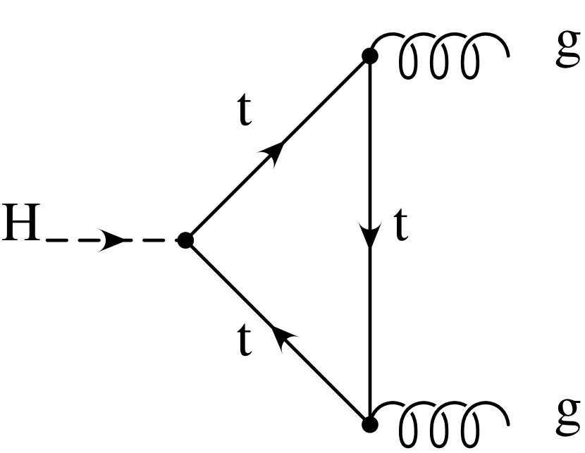
Figure 5.1: Top triangle.

Figure 5.2: $W$ triangle.

Figure 5.3: $W$ bubble.

Figure 5.4: Top triangle.

Figure 5.5: 1st effective $b$-quark decay.

Figure 5.6: 2nd effective $b$-quark decay.

For a two photon Higgs decay, ignoring radiative corrections, one finds [56, 57, 58]

$$\Gamma(H\to\gamma\gamma) = \frac{\alpha^{2}g^{2}}{1024\pi^{3}}\frac{M_{H}^{3}}{M_{W}^{2}}\left|\sum_{i}e_{i}^{2}N_{c\,i}F_{i}\right|^{2}=\frac{\alpha^{2}g^{2}}{1024\pi^{3}}\frac{M_{H}^{3}}{M_{W}^{2}}\left|\frac{4}{3}F_{1/2}+F_{W}\right|^{2}$$ (5.1)

where the functions $F_{1/2}$ and $F_{W}$ are given by

$$F_{1/2} = -2\tau[1+(1-\tau)f(\tau)]$$ (5.2)

and

$$F_{W} = 2+3\tau+3\tau(2-\tau)f(\tau)$$ (5.3)

where $\tau=4m_{i}^{2}/M_{H}^{2}$. The first function corresponds to the contribution of the top quark and the second to the contribution of the charged $W$ bosons. As we assume that the Higgs boson is light, i.e., lighter than twice the mass of the $W$ bosons, the function $f(\tau)$ reads

$$f(\tau) = \left(\arcsin{\left(\sqrt{\frac{1}{\tau}}\right)}\right)^{2}.$$ (5.4)

For the decay into two gluons one finds [56, 57]

$$\Gamma(H\to gg) = \frac{\alpha_{s}^{2}g^{2}}{512\pi^{3}}\frac{M_{H}^{3}}{M_{W}^{2}}\left|F_{1/2}\right|^{2},$$ (5.5)

also neglecting the radiative corrections. The function $F_{1/2}$ was given in equation (5.2).

Another possibility for the Higgs boson to decay are the electroweak boson channels $H\to WW$ and $H\to ZZ$. The Higgs boson couples to the electroweak bosons with the same strength as in the standard model. The decay via two virtual electroweak bosons represents a non-negligible contribution to the Higgs decay. For $m_{W}<m_{H}$ or $m_{Z}<m_{H}$ one of the electroweak bosons is on-shell. These decay rates were evaluated using the program HDECAY [59] and cross-checked using CompHEP [60]. The numerical results are the sum of the decay over two electroweak bosons, for a light Higgs both electroweak bosons are virtual, when allowed by the kinematics, the contributions of on-shell electroweak bosons are also taken into account.

channel	$\!m_{H}\!=\!60$	$\!m_{H}\!=\!70$	$\!m_{H}\!=\!80$	$\!m_{H}\!=\!90$	$\!m_{H}\!=\!100$
$\Gamma(H\!\to\!gg)_{\alpha_{s}=0.119}\!\!$	$2.3\times 10^{-5}$	$3.7\times 10^{-5}$	$5.5\times 10^{-5}$	$7.9\times 10^{-5}$	$1.1\times 10^{-4}$
$\Gamma(H\!\to\!gg)_{\alpha_{s}=0.15}\!\!$	$3.6\times 10^{-5}$	$5.8\times 10^{-5}$	$8.7\times 10^{-5}$	$1.3\times 10^{-4}$	$1.7\times 10^{-4}$
$\Gamma(H\!\to\!\gamma\,\gamma)$	$8.0\times 10^{-7}$	$1.3\times 10^{-6}$	$2.0\times 10^{-6}$	$3.0\times 10^{-6}$	$4.4\times 10^{-6}$
$\Gamma(H\!\to\!W\,W)\!\!$	$1.09\times 10^{-7}$	$3.80\times 10^{-7}$	$1.22\times 10^{-6}$	$4.49\times 10^{-6}$	$2.66\times 10^{-5}$
$\Gamma(H\!\to\!Z\,Z)\!\!$	$3.33\times 10^{-8}$	$1.10\times 10^{-7}$	$3.27\times 10^{-7}$	$9.12\times 10^{-7}$	$2.72\times 10^{-6}$

Table 5.1: Higgs boson decay rates in GeV for different Higgs masses in GeV.

The results of these calculations are given in table 5.1. The corresponding branching ratios are given in table 5.2. We see that such a Higgs boson would decay in a fundamentally different way than the Higgs boson of the standard model. The results for the $H\to gg$ decay are strongly dependent of the value chosen for $\alpha_{s}$. Thus this decay channel has a considerable uncertainty. We have done the calculations for two different values of the strong coupling constant $\alpha_{s}=0.119$ and $\alpha_{s}=0.15$. The fine-structure constant was taken to be $\alpha=1/128.9$.

Even if the light fermions in particular the $b$-quark, do not couple directly to the Higgs boson, some $b$-quarks could be produced via the diagrams 5.6 and 5.6. Their contributions is not easy to estimate but the electroweak corrections for a light Higgs boson are known to be very small [61], typically $0.3\%$ of the tree level value. Nevertheless they could still be of the same order of magnitude as the $\gamma\gamma$ contribution. Above $90$ GeV the decay channel $H\to Z\gamma$ opens. For masses larger than $110$ GeV the Higgs boson mainly decays into two electroweak bosons.

The present searches for the Higgs boson at LEP are mainly based on the assumption that the leading decay made in the mass region of about 100 GeV or less is the decay $H\rightarrow\bar{b}b$. The present experimental limit $m_{H}>113.3$ GeV [62] is obtained on the basis of this assumption. In our model the decay is dominated by the decay $H\rightarrow gg$, i.e., the decay products do not show a specific flavor dependence. The lower limit on the mass of such a boson is much weaker and of the order of $70$ GeV [63].

The best way to detect the Higgs boson at LEP seems to us to search for the decay $H\rightarrow\gamma\gamma$. Since the invariant mass of the $2\gamma$ system would be identical to the mass of the boson, the background coming from radiation effects could be substantially reduced. In our case this decay channel, having a small branching ratio, is not seriously constrained by fermiophobic Higgs studies [62].

Typical fits of the Higgs boson mass indicate that the most likely mass of the boson is about $m_{H}=98^{+58}_{-38}$ GeV [50]. It might well be, that the mass of the Higgs boson is in the region $70$ to $110$ GeV, provided the decay proceeds via the mechanism discussed above. We note that in contrast to the standard expectation the Higgs particle is a relatively narrow object with a width of about $58.5$ KeV.

channel	$\!m_{H}\!=\!60$	$\!m_{H}\!=\!70$	$\!m_{H}\!=\!80$	$\!m_{H}\!=\!90$	$\!m_{H}\!=\!100$
${\mbox{B}r}(H\!\to\!gg)$	$96.06\,\%$	$95.39\,\%$	$93.94\,\%$	$90.39\,\%$	$76.54\,\%$
${\mbox{B}r}(H\!\to\!\gamma\,\gamma)$	$3.34\,\%$	$3.35\,\%$	$3.42\,\%$	$3.43\,\%$	$3.06\,\%$
${\mbox{B}r}(H\!\to\!W\,W)$	$0.46\,\%$	$0.98\,\%$	$2.08\,\%$	$5.14\,\%$	$18.51\,\%$
${\mbox{B}r}(H\!\to\!Z\,Z)$	$0.14\,\%$	$0.28\,\%$	$0.56\,\%$	$1.04\,\%$	$1.89\,\%$

Table 5.2: Branching ratios for different Higgs masses in GeV and for $\alpha_{s}=0.119$.

5.2 Electroweak $d$-waves

In the model considered in chapter 2, new particles corresponding to exotic particles like leptoquarks can be introduced. But, they do not survive to the expansion in $1/F$, and therefore, the duality cannot be applied to describe their properties. Leptoquarks are bound states of two fermions. Forces between two fermions can be very much different than those between a fermion and a scalar or between two scalars. If leptoquarks do exist, their mass scale is presumably very high.

Of particular interest are radially excited versions of the Higgs boson $H^{*}$ and of the electroweak bosons $W^{3*}$ and $W^{\pm*}$. The most promising candidates for energies available at the LHC or at future linear colliders are the excited states of the Higgs boson and of the electroweak bosons. Especially the orbital excitation, i.e., the spin 2 $d$-waves $D^{3}_{\mu\nu}$, $D^{-}_{\mu\nu}$ and $D^{+}_{\mu\nu}$, of the electroweak bosons have a well defined $1/F$ expansion (we use the unitary gauge: $h=(h_{(1)}+F,0)$:

$$D^{3}_{\mu\nu} = \frac{2}{g^{2}F^{2}}\left(\left(D_{\mu}h\right)^{\dagger}\left(D_{\nu}h\right)+\left(D_{\nu}h\right)^{\dagger}\left(D_{\mu}h\right)\right)\approx B^{3}_{\nu}B^{3}_{\mu}+B^{+}_{\nu}B^{-}_{\mu}+B^{+}_{\mu}B^{-}_{\nu}$$ (5.6)

$$D^{-}_{\mu\nu} = \frac{-\sqrt{2}}{g^{2}F^{2}}\epsilon^{ij}\left(\left(D_{\mu}h\right)_{i}\left(D_{\nu}h\right)_{j}+\left(D_{\nu}h\right)_{i}\left(D_{\mu}h\right)_{j}\right)\approx B^{3}_{\mu}B^{-}_{\nu}+B^{3}_{\nu}B^{-}_{\mu}$$

$$D^{+}_{\mu\nu} = \left(\frac{-\sqrt{2}}{g^{2}F^{2}}\epsilon^{ij}\left(\left(D_{\mu}h\right)_{i}\left(D_{\nu}h\right)_{j}+\left(D_{\nu}h\right)_{i}\left(D_{\mu}h\right)_{j}\right)\right)^{\dagger}\approx B^{3}_{\mu}B^{+}_{\nu}+B^{3}_{\nu}B^{+}_{\mu}$$

where $D_{\mu}$ is the covariant derivative, $B_{\mu}^{a}$, $a=\{3,+,-\}$ are the gauge fields and $g$ is the coupling constant corresponding to the gauge group $SU(2)_{L}$. Although the masses and the couplings of these electroweak $d$-waves to other particles are fixed by the dynamics of the model, it is difficult to determine these parameters. In analogy to Quantum Chromodynamics, it is expected that the $d$-waves couple with a reasonable strength to the corresponding $p$-waves, the electroweak bosons. In the following, we assume in accordance with the duality property, that the $d$-waves only couple to the electroweak bosons and not to the photon, the Higgs boson or the fermions.

5.3 Production of the electroweak $d$-waves

The cross-sections and decay width of $d$-waves predicted in a variety of composite models were considered in [64]. Here we shall consider different effective couplings of our electroweak $d$-waves that are more suitable for the model proposed in chapter 2. If their masses are of the order of the scale of the theory, they will be accessible at the LHC. Of particular interest is the neutral electroweak $d$-wave because it is expected to couple to the $W^{\pm}$ electroweak bosons. This particle can thus be produced by the fusion of two electroweak bosons at the LHC or at linear colliders.

We shall use the formalism developed by van Dam and Veltman [65] for massive $d$-waves to compute the decay width of the $D^{3}_{\mu\nu}$ into $W^{+}W^{-}$. We use the following relation:

$$\sum^{5}_{i=1}e^{i}_{\mu\nu}(p)e^{i}_{\alpha\beta}(p) = \frac{1}{2}\left(\delta_{\mu\alpha}\delta_{\nu\beta}+\delta_{\mu\beta}\delta_{\nu\alpha}-\delta_{\mu\nu}\delta_{\alpha\beta}\right)$$

$$+\frac{1}{2}\left(\delta_{\mu\alpha}\frac{p_{\nu}p_{\beta}}{m_{D}^{2}}+\delta_{\nu\beta}\frac{p_{\mu}p_{\alpha}}{m_{D}^{2}}+\delta_{\mu\beta}\frac{p_{\nu}p_{\alpha}}{m_{D}^{2}}+\delta_{\nu\alpha}\frac{p_{\mu}p_{\beta}}{m_{D}^{2}}\right)$$

$$+\frac{2}{3}\left(\frac{1}{2}\delta_{\mu\nu}-\frac{p_{\mu}p_{\nu}}{m_{D}^{2}}\right)\left(\frac{1}{2}\delta_{\alpha\beta}-\frac{p_{\alpha}p_{\beta}}{m_{D}^{2}}\right)$$

for the sum over the polarizations $e^{i}_{\mu\nu}$ of the $d$-wave. In the notation of [65] the sum over the polarizations of the $W^{\pm}$ is given by

$$\sum^{3}_{i=1}e^{i}_{\mu}(p)e^{i}_{\nu}(p) = \delta_{\mu\nu}+\frac{p_{\mu}p_{\nu}}{m_{W}^{2}}$$ (5.8)

where $\delta_{\mu\nu}$ is the Euclidean metric. Averaging over the polarizations of the $d$-wave, we obtain

$$\Gamma(D^{3}\rightarrow W^{+}W^{-}) = \frac{g^{2}_{D}}{1920m_{D}\pi}\left(x_{W}-4\right)^{2}\sqrt{\left(1-\frac{4}{x_{W}}\right)}$$ (5.9)

with $x_{W}=(m_{D}/m_{W})^{2}$, where $m_{D}$ is the mass of the $d$-wave and $g_{D}$ is a dimensionfull coupling constant with $\mbox{dim}[g_{D}]=\mbox{GeV}$. A dimensionless coupling constant is obtained by a redefinition of the coupling constant $g_{D}\rightarrow m_{D}\bar{g}_{D}$. We shall discuss plausible numerical inputs in the next section. Assuming that the $Z$ boson couples with the same strength to the $d$-wave as the $W$-bosons, we can estimate the decay width into $Z$ bosons in the following way

$$\Gamma(D^{3}\rightarrow ZZ) = \frac{g^{2}_{D}}{3840m_{D}\pi}\left(x_{Z}-4\right)^{2}\sqrt{\left(1-\frac{4}{x_{Z}}\right)}$$

$$\approx \frac{1}{2}\Gamma(D^{3}\rightarrow W^{+}W^{-})$$

with $x_{Z}=(m_{D}/m_{Z})^{2}$. The Breit-Wigner resonance cross section for the reaction $W^{+}+W^{-}\rightarrow D^{3}$ thus reads (see e.g. [66])

$$\sigma^{(res)}_{W^{+}+W^{-}\rightarrow D^{3}} = \frac{10\pi}{q^{2}}\frac{m_{D}^{2}\Gamma^{\mbox{(tot)}}_{D}\Gamma(D^{3}\rightarrow W^{+}W^{-})}{\left(m_{D}^{2}-s\right)^{2}+m_{D}^{2}{\Gamma^{\mbox{(tot)}}_{D}}^{2}}$$ (5.11)

where $q^{2}=(s-4m_{W}^{2})/4$ and $\Gamma^{(\mbox{tot})}_{D}\approx 3/2\Gamma(D^{3}\rightarrow W^{+}W^{-})$ is the total decay width of the neutral $d$-wave. Due to the background, the $W$ bosons might be difficult to observe. But, if the electroweak $d$-waves states are produced we also expect an excess of $Z$ bosons compared to the standard model expectation. Note that the $Z$ bosons are easier to observe.

As we shall see in the next section, the neutral $d$-waves give a sizable contribution to the reaction $W^{+}+W^{-}\to W^{+}+W^{-}$.

5.4 The reaction $W^{+}+W^{-}\to W^{+}+W^{-}$

A considerable attention has been paid to the scattering of electroweak bosons since this represents a stringent test of the gauge structure of the standard model. In particular the reaction $W^{+}+W^{-}\to W^{+}+W^{-}$ is of prime interest. If the Higgs boson is heavier than 1 TeV, the electroweak bosons will start to interact strongly [67]. This reaction has been studied in the framework of the standard model in [68]. The one loop corrections were considered in [69] and are known to be sizable. For the sake of this work, the tree level diagrams are sufficient to show that the contribution of the neutral electroweak $d$-wave will be sizable and cannot be overlooked in forthcoming experiments. As described in [57] (see also [68]) the $W$’s emitted by the beam particles are dominantly longitudinally polarized if the following relations are fulfilled: $m_{W}^{2}\ll m^{2}_{WW}\ll s$ at an $e^{+}$ $e^{-}$ collider, and $m_{W}^{2}\ll m^{2}_{WW}\ll s_{q\bar{q}}\ll s$ at a hadron collider, and we shall only consider the especially interesting reaction $W^{+}_{L}+W^{-}_{L}\to W^{+}_{L}+W^{-}_{L}$ as described in [68]. In the standard model, this reaction is a test of the gauge structure of the theory [55]. The Feynman graphs contributing in the standard model to this reaction can be found in figures 5.9, 5.9, 5.9, 5.11 and 5.11.

Figure 5.7: photon and Z boson in the s channel

Figure 5.8: photon and Z boson in the t channel

Figure 5.9: four W vertex

Figure 5.10: Higgs boson in the s channel

Figure 5.11: Higgs boson in the t channel

The amplitudes corresponding to these graphs are [68]

$$A_{s\gamma} = -\frac{1}{16}ig^{2}xs^{2}\beta^{2}(3-\beta^{2})^{2}\cos{\theta},$$ (5.12)

$$A_{sZ} = -\frac{1}{16}ig^{2}(1-x)\frac{s^{3}}{s-\xi_{Z}}\beta^{2}(3-\beta^{2})^{2}\cos{\theta},$$

$$A_{t\gamma} = -\frac{1}{32}ig^{2}x\frac{s^{3}}{t}[\beta^{2}(4-2\beta^{2}+\beta^{4})+\beta^{2}(4-10\beta^{2}+\beta^{4})\cos{\theta}$$

$$+(2-11\beta^{2}+10\beta^{4})\cos^{2}{\theta}+\beta^{2}\cos^{3}{\theta}],$$

$$A_{tZ} = -\frac{1}{32}ig^{2}(1-x)\frac{s^{3}}{t-\xi_{Z}}[\beta^{2}(4-2\beta^{2}+\beta^{4})+\beta^{2}(4-10\beta^{2}+\beta^{4})\cos{\theta}$$

$$+(2-11\beta^{2}+10\beta^{4})\cos^{2}{\theta}+\beta^{2}\cos^{3}{\theta}],$$

$$A_{4} = -\frac{1}{16}ig^{2}s^{2}(1+2\beta^{2}-6\beta^{2}\cos{\theta}-\cos^{2}{\theta}),$$

$$A_{sH} = -\frac{1}{16}ig^{2}s^{2}\frac{(1+\beta^{2})^{2}}{s-\xi_{H}+i\gamma_{H}},$$

$$A_{tH} = -\frac{1}{16}ig^{2}s^{2}\frac{(\beta^{2}-\cos{\theta})^{2}}{t-\xi_{H}+i\gamma_{H}},$$

where $x=\sin^{2}{\theta_{W}}$, $\xi_{Z}=(1-x)^{-1}=m_{Z}^{2}/m^{2}_{W}$, $\xi_{H}=m_{H}^{2}/m^{2}_{W}$, $\gamma_{H}=m_{H}\Gamma_{H}/m_{W}^{2}$ and $\beta=\sqrt{1-4/s}$. The variables $s$ and $t$ are scaled with respect to $m_{W}^{2}$. The scattering angle is $\theta$, $t=-1/2s\beta^{2}(1-\cos{\theta})$. These notations are the same as those introduced in [68]. The standard model amplitude is thus

$$A^{sum}_{SM} = A_{s\gamma}+A_{sZ}+A_{t\gamma}+A_{tZ}+A_{4}+A_{sH}+A_{tH}.$$ (5.13)

In the high energy limit, one observes the cancellation of the leading powers in $s$ and finds [68]

$$A^{sum}_{SM}\approx\frac{1}{2}ig^{2}\left[\xi_{Z}\left(1+\frac{s}{t}+\frac{t}{s}\right)+\xi_{H}-i\gamma_{H}\right]$$ (5.14)

for the sum of these amplitudes. The cross section with the angular cut $-z_{0}<\cos\theta<z_{0}$ is then

$$\sigma = \frac{1}{16\pi s^{2}\beta^{2}}\int^{t_{+}}_{t_{-}}|A^{sum}|^{2}\mbox{d}t$$ (5.15)

in dimensionless units, $t_{\pm}=(2-s/2)(1\mp z_{0})$.

The excitations of the Higgs and electroweak bosons also contribute via the $s$ and $t$ channel. The amplitudes corresponding to the contribution of a radially excited Higgs boson ($H^{*}$) of mass $m_{H^{*}}$ and decay width $\Gamma_{H^{*}}$ to this reaction are

$$A_{sH^{*}} = -\frac{1}{16}ig^{2}_{H^{*}}s^{2}\frac{(1+\beta^{2})^{2}}{s-\xi_{H^{*}}+i\gamma_{H^{*}}},$$ (5.16)

$$A_{tH^{*}} = -\frac{1}{16}ig^{2}_{H^{*}}s^{2}\frac{(\beta^{2}-\cos{\theta})^{2}}{t-\xi_{H^{*}}+i\gamma_{H^{*}}},$$

where $\xi_{H^{*}}=m_{H^{*}}^{2}/m^{2}_{W}$, $\gamma_{H^{*}}=m_{H^{*}}\Gamma_{H^{*}}/m_{W}^{2}$ and $g_{H^{*}}$ is the strength of the coupling between two $W$ bosons and the $H^{*}$ scalar particle.

We shall now consider the contribution of the radially $(W^{3*})$ and orbitally $(D^{\mu\nu})$ excited neutral $Z$ boson. The amplitudes for the $W^{3*}$ can be at once deduced from those of the standard model contribution of the $Z$ boson

$$A_{sW^{3*}} = -\frac{1}{16}ig^{2}_{W^{3*}}\frac{s^{3}}{s-\xi_{W^{3*}}+i\gamma_{W^{3*}}}\beta^{2}(3-\beta^{2})^{2}\cos{\theta},$$ (5.17)

$$A_{tW^{3*}} = -\frac{1}{32}ig^{2}_{W^{3*}}\frac{s^{3}}{t-\xi_{W^{3*}}+i\gamma_{W^{3*}}}[\beta^{2}(4-2\beta^{2}+\beta^{4})$$

$$+\beta^{2}(4-10\beta^{2}+\beta^{4})\cos{\theta}+(2-11\beta^{2}+10\beta^{4})\cos^{2}{\theta}+\beta^{2}\cos^{3}{\theta}],$$

where $\xi_{W^{3*}}=m_{W^{3*}}^{2}/m^{2}_{W}$, $\gamma_{W^{3*}}=m_{W^{3*}}\Gamma_{W^{3*}}/m_{W}^{2}$ and $g_{W^{3*}}$ is the strength of the coupling between two $W$ bosons and the $W^{3*}$ boson.

The orbitally excited $Z$ boson $(D^{\mu\nu})$ is a $d$-wave, and its propagation is thus described by a propagator corresponding to a massive spin 2 particle. The propagator of a massive spin two particle is as follows (see [65]):

$$\Gamma_{\mu\nu\rho\sigma} = \frac{1}{p^{2}-m_{D}^{2}}\frac{1}{2}(g_{\mu\rho}g_{\nu\sigma}+g_{\mu\sigma}g_{\nu\rho}-\frac{2}{3}g_{\mu\nu}g_{\rho\sigma})$$ (5.18)

and we assume that the vertex $W^{+\mu}W^{-\nu}D_{\mu\nu}$ is of the form $ig_{D}$. We obtain the following amplitudes for the $s$ and $t$ channel exchange

$$A_{sD} = \frac{-1}{48}ig_{D}^{2}\frac{m_{D}^{2}}{m_{W}^{2}}\frac{s^{2}}{s-\xi_{D}+i\gamma_{D}}\left(2\beta^{4}+3\cos^{2}{\theta}-2\beta^{2}-1\right)$$ (5.19)

$$\!\!\!\!\!\!\!\!\!A_{tD} = \frac{-1}{96}ig_{D}^{2}\frac{m_{D}^{2}}{m_{W}^{2}}\frac{s^{2}}{t-\xi_{D}+i\gamma_{D}}\left(4\beta^{4}+6\beta^{2}+3+10\beta^{2}\cos{\theta}+1\cos{\theta}^{2}\right).$$ (5.20)

Since there is a pole in the $t$ channel whose origin is the photon exchange, one has to impose cuts on the cross sections. For the numerical evaluation of the cross section, we impose a cut of $10^{\circ}$, which is the cut chosen in [69]. The spin of the particle can be determined from the angular distribution of the cross section. We have neglected the decay width of the $Z$ boson and that of the Higgs boson since we assume that the energy of the process is such that no $Z$ boson or Higgs resonance appear. For numerical estimates, we take $m_{H}=100$ GeV.

We have considered only the reaction involving longitudinally polarized $W$. The amplitudes for different polarizations for the standard model can be found in the literature [68]. The amplitudes for a $H^{*}$ or a $W^{3*}$ can be deduced from the standard model calculations by replacing the masses, the decay widths and the coupling constants. Those for the neutral $d$-wave can be easily calculated using

$${\cal A}^{p_{1}p_{2}p_{3}p_{4}}_{s} = -ig_{D}^{2}\frac{m_{D}^{2}}{m_{W}^{2}}\frac{1}{s-\xi_{D}+i\gamma_{D}}$$

$$\frac{1}{2}\epsilon^{\mu}(p_{1})\epsilon^{\nu}(p_{2})(g_{\mu\rho}g_{\nu\sigma}+g_{\mu\sigma}g_{\nu\rho}-\frac{2}{3}g_{\mu\nu}g_{\rho\sigma})\epsilon^{*\rho}(p_{3})\epsilon^{*\sigma}(p_{4})$$

and

$${\cal A}^{p_{1}p_{2}p_{3}p_{4}}_{t} = -ig_{D}^{2}\frac{m_{D}^{2}}{m_{W}^{2}}\frac{1}{t-\xi_{D}+i\gamma_{D}}$$

$$\frac{1}{2}\epsilon^{\mu}(p_{1})\epsilon^{\rho}(p_{2})(g_{\mu\rho}g_{\nu\sigma}+g_{\mu\sigma}g_{\nu\rho}-\frac{2}{3}g_{\mu\nu}g_{\rho\sigma})\epsilon^{*\nu}(p_{3})\epsilon^{*\sigma}(p_{4})$$

where $p_{i}$ stands for the polarization and also using the following relations

$$\epsilon^{\mu}_{1}(0)=(-p,0,0,E)/m_{W} \epsilon^{\mu}_{1}(\pm)=(0,-1,\pm i,0)/\sqrt{2}$$

$$\epsilon^{\mu}_{2}(0)=(-p,0,0,-E)/m_{W} \epsilon^{\mu}_{2}(\pm)=(0,1,\pm i,0)/\sqrt{2}$$

$$\epsilon^{*\mu}_{3}(0)=(p,-E\sin{\theta},0,-E\cos{\theta})/m_{W} \epsilon^{*\mu}_{3}(\pm)=(0,-\cos{\theta},\mp i,\sin{\theta})/\sqrt{2}$$

$$\epsilon^{*\mu}_{4}(0)=(p,E\sin{\theta},0,E\cos{\theta})/m_{W} \epsilon^{*\mu}_{4}(\pm)=(0,\cos{\theta},\mp i,-\sin{\theta})/\sqrt{2}$$

valid in the center of mass system where $E$ is the energy of the $W$ bosons, $p=\sqrt{E^{2}-m_{W}^{2}}$ is their momentum and $\theta$ is the scattering angle.

5.5 Discussion

The differential cross section for the reaction $W_{L}^{+}W_{L}^{-}\to W_{L}^{+}+W_{L}^{-}$ can be found in figure 5.12 for the reaction involving the neutral $d$-wave, figure 5.13 for that involving the $W^{3*}$ spin 1 boson and figure 5.14 for that involving the $H^{*}$ scalar. The particles $W^{3*}$ and $H^{*}$ are assumed to couple, in a first approximation, only to the $W$’s. This allows to compute their decay rates using standard model formulas. As mentioned previously, it is not an easy task to predict the mass spectrum of the model, thus we assumed, for numerical illustration, three different masses: 350 GeV, 500 GeV and 800 GeV. The coupling constants are assumed to sizable (see the figures 5.12, 5.13, 5.14 and 5.15). If the cross sections are extrapolated to very high energies, unitarity is violated. However, as expected in any substructure models, it will be restored by bound states effects.

It is very instructive to plot the ratio of the differential cross section involving new physics to the standard model differential cross section. We have done so for the neutral $d$-wave (fig. 5.15). It is obvious from this picture that any deviation from the standard model, even at high energy will manifest itself already in a deviation from one for that ratio. Already at an energy which is low compared to the mass of the new particle, i.e. well bellow the resonance, one observes a deviation from unity.

Nevertheless the calculation of the full reaction e.g. $e^{+}e^{-}\to W^{+}W^{-}\nu\bar{\nu}$ involves the convolution of the cross section of the reaction $W^{+}W^{-}\to W^{+}+W^{-}$ with functions describing the radiative emission of the $W$’s from the fermions. When this integral is performed some sensitivity is lost. Nevertheless the effects are expected to be so large that they cannot be overlooked. The reaction will allow to test a mass range of a few TeV’s so that even if the new particles are too massive to be produced on-shell, their effects will be noticeable at future colliders.

Figure 5.12: Dimensionless cross section of the reaction $W_{L}^{+}W_{L}^{-}\to W_{L}^{+}+W_{L}^{-}$ including the $d$-wave. The solid line is the standard model cross section, the dotted line corresponds to a $d$-wave of mass 350 GeV, with $\Gamma=4.38$ GeV and $\bar{g}_{W^{3*}}=0.8g$, the long dashed line to a $d$-wave of mass 500 GeV, with $\Gamma=27.49$ GeV and $\bar{g}_{W^{3*}}=0.7g$ and the dot-dashed line to a $d$-wave of mass 800 GeV, with $\Gamma=251.03$ GeV and $\bar{g}_{W^{3*}}=0.6g$.

Figure 5.13: Dimensionless cross section of the reaction $W_{L}^{+}W_{L}^{-}\to W_{L}^{+}+W_{L}^{-}$ including the $W^{3*}$ boson. The solid line is the standard model cross section, the dotted line corresponds to a $W^{3*}$ boson of mass 350 GeV, with $\Gamma=66.2$ GeV and $\bar{g}_{W^{3*}}=0.8\sin^{2}{\theta_{W}}g$, the long dashed line to a $W^{3*}$ boson of mass 500 GeV, with $\Gamma=266.8$ GeV and $\bar{g}_{W^{3*}}=0.7\sin^{2}{\theta_{W}}g$ and the dot-dashed line to a $W^{3*}$ boson of mass 800 GeV, with $\Gamma=1795.5$ GeV and $\bar{g}_{W^{3*}}=0.6\sin^{2}{\theta_{W}}g$.

Figure 5.14: Dimensionless cross section of the reaction $W_{L}^{+}W_{L}^{-}\to W_{L}^{+}+W_{L}^{-}$ including the $H^{*}$ boson. The solid line is the standard model cross section, the dotted line corresponds to a $H^{*}$ boson of mass 350 GeV, with $\Gamma=6.72$ GeV and $\bar{g}_{H^{*}}=0.8g$, the long dashed line to a $H^{*}$ boson of mass 500 GeV, with $\Gamma=17.6$ GeV and $\bar{g}_{H^{*}}=0.7g$ and the dot-dashed line to a $W^{3*}$ boson of mass 800 GeV, with $\Gamma=58.25$ GeV and $\bar{g}_{H^{*}}=0.6g$.

Figure 5.15: Ratio of the cross-section for the of the reaction involving the $d$-wave to the standard model cross-section for different values of the $d$-wave mass and different coupling constants. The dotted line corresponds to a $d$-wave of mass 350 GeV, with $\Gamma=4.38$ GeV and $\bar{g}_{W^{3*}}=0.8g$, the long dashed line to a $d$-wave of mass 500 GeV, with $\Gamma=27.49$ GeV and $\bar{g}_{W^{3*}}=0.7g$ and the dot-dashed line to a $d$-wave of mass 800 GeV, with $\Gamma=251.03$ GeV and $\bar{g}_{W^{3*}}=0.6g$.

5.6 Conclusions

We have discussed the production of a neutral $d$-wave $D^{3}$ at the LHC or at a linear collider. If the mass of this particle is of the order of the scale of the theory, i.e. 300 GeV, it can be produced at these colliders. We have also shown that this particle as well as radial excitations of the Higgs boson and $Z$ boson would spoil the cancellation of the leading powers in $s$ of in the reaction $W^{+}_{L}+W^{-}_{L}\to W^{+}_{L}+W^{-}_{L}$, thus any new particle contributing to that reaction will have a large impact already at energies well below the mass of this new particle. This reaction is thus not only of prime interest if the Higgs boson is heavy but should also be studied if the Higgs boson was light.

Chapter 6 The substructure of fermions

If the duality breaks down entirely at a certain energy scale, it is conceivable that effects from the substructure of the fermions will become manifest. We shall discuss a quite generic parametrization of the contribution of the substructure of a lepton to its anomalous magnetic moment. Assuming a mixing matrix, we can then consider radiative lepton decays that are conceivable if leptons have a substructure. The results presented in this chapter were published in [70, 71].

6.1 Anomalous magnetic moment

A new contribution to the magnetic moment of the muon can be described by adding an effective term ${\cal L}^{eff}$ to the Lagrangian of the standard model as follows:

$${\cal L}^{eff} = \frac{e}{2\Lambda}\bar{\mu}\left(A+B\gamma_{5}\right)\sigma_{\mu\nu}\mu F^{\mu\nu}\left(1-\frac{4\alpha}{\pi}\ln\frac{\Lambda}{m_{\mu}}\right),$$ (6.1)

where $\mu$ is the muon field, $F^{\mu\nu}$ the electromagnetic field strength, $\Lambda$ the compositeness scale and $A$ is a constant of order one and $B$ is probably much smaller since it parametrizes $CP$-violation. We have taken the QED one loop correction into account [72]. The leading order contribution has been considered in [70]. We have included a $\gamma_{5}$-term in view of a possible $CP$ violation of the confining interaction.

The constants in ${\cal L}^{eff}$ depend on dynamical details of the underlying composite structure. If the latter is analogous to QCD, where such a term is induced by the hadronic dynamics, the constant $A$ is of the order one. One obtains the following contribution to the anomalous magnetic moment of the muon:

$$\Delta a_{\mu} = \left(\frac{m_{\mu}}{\Lambda}\right)\left(1-\frac{4\alpha}{\pi}\ln\frac{\Lambda}{m_{\mu}}\right).$$ (6.2)

The $\gamma_{5}$-term does not contribute to the anomalous magnetic moment.

The magnetic moment term (6.1) has the same chiral structure as the lepton mass term. Thus one expects that the same mechanism which leads to the small lepton masses ($m_{\mu}\ll\Lambda$), e.g. a chiral symmetry, leads to a corresponding suppression of the magnetic moment [73]. In this case the effective Lagrangian should be written as follows:

$${\cal L}^{eff} = \frac{e}{2\Lambda}\frac{m_{\mu}}{\Lambda}\bar{\mu}\left(A+B\gamma_{5}\right)\sigma_{\mu\nu}\mu F^{\mu\nu}\left(1-\frac{4\alpha}{\pi}\ln\frac{\Lambda}{m_{\mu}}\right).$$ (6.3)

The contribution of the compositeness to the magnetic moment is in this case given by

$$\Delta a_{\mu} = \left(\frac{m_{\mu}}{\Lambda}\right)^{2}\left(1-\frac{4\alpha}{\pi}\ln\frac{\Lambda}{m_{\mu}}\right).$$ (6.4)

6.2 Radiative lepton decays

If the leptons have a composite structure, the question arises whether effects which are absent in the standard model, in particular flavor-changing transitions, e.g. the decays $\mu\to e\gamma$ or $\tau\to\mu\gamma$ arise.

We shall study flavor changing magnetic-moment type transitions which indeed lead to radiative decays of the charged leptons on a level accessible to experiments in the near future.

We start by considering the limit $m_{e}=m_{\mu}=0$, i.e. only the third lepton $\tau$ remains massive. Neutrino masses are not considered. In this limit the mass matrix for the charged leptons has the structure $m_{l^{-}}=m_{\tau}\mbox{diag}(0,0,1)$ and exhibits a “democratic symmetry” [74, 75]. Furthermore there exists a chiral symmetry $SU(2)_{L}\times SU(2)_{R}$ acting on the first two lepton flavors. The magnetic moment term induced by compositeness, being of a similar chiral nature as the mass term itself, must respect this symmetry. We obtain

$${\cal L}^{eff} = \frac{e}{2\Lambda}\frac{m_{\tau}}{\Lambda}\bar{\psi}\tilde{M}\left(A+B\gamma_{5}\right)\sigma_{\mu\nu}\psi F^{\mu\nu}\left(1-\frac{4\alpha}{\pi}\ln\frac{\Lambda}{m_{\psi}}\right).$$ (6.5)

Here $\psi$ denotes the vector $(e,\mu,\tau)$ and $\tilde{M}$ is given by $\tilde{M}=\mbox{diag}(0,0,1)$.

Once the chiral symmetry is broken, the mass matrix receives non-zero entries, and after diagonalization by suitable transformations in the space of the lepton flavors it takes the form $M=\mbox{diag}(m_{e},m_{\mu},m_{\tau})$. If after symmetry breaking the mass matrix $M$ and the magnetic moment matrix $\tilde{M}$ were identical, the same diagonalization procedure which leads to a diagonalized mass matrix would lead to a diagonalized magnetic moment matrix. However there is no reason why $\tilde{M}$ and $M$ should be proportional to each other after symmetry breaking. The matrix elements of the magnetic moment operator depend on details of the internal structure in a different way than the matrix elements of the mass density operator. Thus in general the magnetic moment operator will not be diagonal, once the mass matrix is diagonalized and vice versa. Thus there exist flavor-non-diagonal terms (for a discussion of analogous effects for the quarks see [74]), e.g. terms proportional to $\bar{e}\ \sigma_{\mu\nu}\left(A+B\gamma_{5}\right)\mu$. These flavor-non-diagonal terms must obey the constraints imposed by the chiral symmetry, i.e. they must disappear once the masses of the light leptons involved are turned off. For example, the $e-\mu$ transition term must vanish for $m_{e}\to 0$. Furthermore the flavor changing terms arise due to a mismatch between the mass density and the magnetic moment operators due to the internal substructure. If the substructure were turned off ($\Lambda\to\infty$), the effects should not be present. The simplest Ansatz for the transition terms between the leptons flavors $i$ and $j$ is $const.\sqrt{m_{i}m_{j}}/\Lambda$. It obeys the constraints mentioned above: it vanishes once the mass of one of the leptons is turned off, it is symmetric between $i$ and $j$ and it vanishes for $\Lambda\to\infty$. In this case the magnetic moment operator has the general form:

$$\!\!\!\!\!\!\!\!{\cal L}^{eff} = \frac{e}{2\Lambda}\frac{m_{\tau}}{\Lambda}\bar{\psi}\left(\begin{array}[]{ccc}\frac{m_{e}}{m_{\tau}}&C_{e\mu}\frac{\sqrt{m_{e}m_{\mu}}}{\Lambda}&C_{e\tau}\frac{\sqrt{m_{e}m_{\tau}}}{\Lambda}\\ C_{e\mu}\frac{\sqrt{m_{e}m_{\mu}}}{\Lambda}&\frac{m_{\mu}}{m_{\tau}}&C_{\mu\tau}\frac{\sqrt{m_{\mu}m_{\tau}}}{\Lambda}\\ C_{e\tau}\frac{\sqrt{m_{e}m_{\tau}}}{\Lambda}&C_{\mu\tau}\frac{\sqrt{m_{\mu}m_{\tau}}}{\Lambda}&1\par\end{array}\right)\psi\left(A+B\gamma_{5}\right)\sigma_{\mu\nu}F^{\mu\nu}$$ (6.10)

$$\times\left(1-\frac{4\alpha}{\pi}\ln\frac{\Lambda}{m_{\psi}}\right).$$

Here $C_{ij}$ are constants of the order one. In general one may introduce two different matrices (with different constants $C_{ij}$) both for the 1-term and for the $\gamma_{5}$-term, but we shall limit ourselves to the simpler structure given above.

Based on the flavor-changing transition terms given in eq. (6.10), we can calculate the decay rates for the decays $\mu\to e\gamma$, $\tau\to\mu\gamma$ and $\tau\to e\gamma$. We find:

$$\Gamma(\mu\to e\gamma) = e^{2}\frac{m_{\mu}}{8\pi}\left(\frac{\sqrt{m_{\mu}m_{e}}}{\Lambda}\right)^{2}\left(\frac{m_{\mu}}{\Lambda}\right)^{2}\left(\frac{m_{\tau}}{\Lambda}\right)^{2}\left(|A|^{2}+|B|^{2}\right)$$ (6.11)

$$\times\left(1-\frac{8\alpha}{\pi}\ln\frac{\Lambda}{m_{\mu}}\right),$$

$$\Gamma(\tau\to\mu\gamma) = e^{2}\frac{m_{\tau}}{8\pi}\left(\frac{\sqrt{m_{\tau}m_{\mu}}}{\Lambda}\right)^{2}\left(\frac{m_{\tau}}{\Lambda}\right)^{2}\left(\frac{m_{\tau}}{\Lambda}\right)^{2}\left(|A|^{2}+|B|^{2}\right)$$ (6.12)

$$\times\left(1-\frac{8\alpha}{\pi}\ln\frac{\Lambda}{m_{\tau}}\right),$$

$$\Gamma(\tau\to e\gamma) = e^{2}\frac{m_{\tau}}{8\pi}\left(\frac{\sqrt{m_{\tau}m_{e}}}{\Lambda}\right)^{2}\left(\frac{m_{\tau}}{\Lambda}\right)^{2}\left(\frac{m_{\tau}}{\Lambda}\right)^{2}\left(|A|^{2}+|B|^{2}\right)$$ (6.13)

$$\times\left(1-\frac{8\alpha}{\pi}\ln\frac{\Lambda}{m_{\tau}}\right).$$

In the following we take $|A|=1$. The parameter $|B|$ can be constrained using the limits for the electron EDM. This limit gives the most stringent constraint on this parameter.

Recently an indication was found that the anomalous magnetic moment of the muon $\mu^{+}$ is slightly larger than expected within the standard model [76]. The deviation is of the order of $10^{-9}$:

$$\Delta a_{\mu} = a_{\mu}(exp)-a_{\mu}(SM)=(4.3\pm 1.6)\times 10^{-9}.$$ (6.14)

For a review of the contribution of the standard model to the anomalous magnetic moment of the muon see Ref. [77]. The observed effect (2.6 $\sigma$ excess) does not necessarily imply a conflict with the standard model, in view of the systematic uncertainties in the theoretical calculations due to the hadronic corrections. If this result is confirmed by further experimental data and theoretical work, it might be interpreted as the first signal towards an internal structure of the leptons [79], although other interpretations (vertex corrections due to new particles or non-minimal couplings due to a more complex space-time structure [80]) are also possible.

The BNL result would give: $\Lambda\approx 2\times 10^{9}$ GeV using eq. (6.2). Using eq. (6.4) and the central value of $\Delta a_{\mu}$, one obtains: $\Lambda\approx 1.54$ TeV, i.e. $\Lambda$ is much smaller due to the chiral symmetry argument [73]. The $95\%$ confidence level range for $\Lambda$ is

$$1.16\ \mbox{TeV}<\Lambda<3.04\ \mbox{TeV}.$$ (6.15)

We can use this experimental input to illustrate the contribution of the fermion substructure to its anomalous magnetic moment and to compute the

The Lagrangian (6.10) yields the following EDM for the electron:

$$d_{e} = \frac{e}{\Lambda}\frac{m_{e}}{\Lambda}|B|\left(1-\frac{4\alpha}{\pi}\ln\frac{\Lambda}{m_{e}}\right)=3.7\times 10^{-24}|B|\mbox{\ e-cm},$$ (6.16)

which has to be compared to the experimental limit ${d_{e}}^{\mbox{exp}}<(0.18\pm 0.12\pm 0.10)\times 10^{-26}e-\mbox{cm}$ [78], we thus see that $|B|$ must be much smaller than $|A|$. We set $|B|=0$ in the following. The corresponding branching ratios are:

$$\mbox{Br}(\mu\to e\gamma) \approx 1.5\times 10^{-10},$$ (6.17)

$$\mbox{Br}(\tau\to\mu\gamma) \approx 3.5\times 10^{-10},$$ (6.18)

$$\mbox{Br}(\tau\to e\gamma) \approx 1.7\times 10^{-12},$$ (6.19)

using the central value of $\Delta a_{\mu}$ to evaluate $\Lambda$. One obtains the following ranges for the branching ratios

$$8.3\times 10^{-10} >\mbox{Br}(\mu\to e\gamma) >2.5\times 10^{-12},\ \ \ \$$ (6.20)

$$1.9\times 10^{-9} >\mbox{Br}(\tau\to\mu\gamma) >5.8\times 10^{-12},$$ (6.21)

$$9.3\times 10^{-12} >\mbox{Br}(\tau\to e\gamma) >2.8\times 10^{-14},$$ (6.22)

using the $95\%$ confidence level range for $\Lambda$ (6.15).

These ranges are based on the assumption that the constant $A$ of order one is fixed to one. The upper part of the range for the $\mu\to e\gamma$ decay given in (6.20) is excluded by the present experimental limit: $\mbox{Br}(\mu\to e\gamma)<1.2\times 10^{-11}$ [78]. Our estimates of the branching ratio should be viewed as order of magnitude estimates. In general we can say that the branching ratio for the $\mu\to e\gamma$ decay should lie between $10^{-13}$ and the present limit.

The decay $\tau\to\mu\gamma$ processes at a level which cannot be observed, at least not in the foreseeable future. The decay $\tau\to e\gamma$ is, as expected, much suppressed compared to $\tau\to\mu\gamma$ decay and cannot be seen experimentally.

Numerically, the effect of the QED one loop correction is small compared to the “tree level” calculation [70] because there is a cancellation between two effects: the extracted composite scale is larger but the decay rates are suppressed by the factor $\left(1-\frac{8\alpha}{\pi}\ln\frac{\Lambda}{m_{f}}\right)$, where $m_{f}$ is the mass of the decaying lepton.

Note added: the QCD uncertainties finally settled down [81, 82, 83, 84]. The deviation is only of the order of 1.6 $\sigma$ which allows to put a limit of 2 TeV for the compositeness scale of the muon. This scale corresponds to the following branching ratios

$$\mbox{Br}(\mu\to e\gamma) \approx 3.1\times 10^{-11},$$ (6.23)

$$\mbox{Br}(\tau\to\mu\gamma) \approx 7.1\times 10^{-11},$$ (6.24)

$$\mbox{Br}(\tau\to e\gamma) \approx 3.5\times 10^{-13},$$ (6.25)

for the radiative lepton decays.

Chapter 7 Conclusions

We have presented a duality between the standard model and a model based on the same gauge group but where $SU(2)_{L}$ is confining its charges instead of being broken by means of the Higgs mechanism. This duality allows a calculation of the electroweak mixing angle and of the mass of the Higgs boson.

If the duality is unbroken, we do not expect any physics beyond the standard model, as both phases are identical. But, both the confinement phase and the Higgs phase are necessary to extracted all the informations present in the theory. Left-handed particles, the electroweak bosons and the Higgs boson have a point like and a bound state like character. The duality allows a calculation of the electroweak mixing angle and of the Higgs boson mass.

We have considered a supersymmetric extension of the duality, and shown that our ideas are compatible with a supersymmetric extension.

Albeit the author does not expect it, this duality might only be a low energy phenomenon. If the standard model breaks down in the Yukawa sector and if Nature is described by the confinement phase, the decay modes of the Higgs boson can be dramatically affected. In particular it might not couple to $b$-quarks. In that case the decay channels of the Higgs boson would differ strongly from the standard model expectations. The strategy for the Higgs boson searches would differ from the standard one. Instead of searching for decays of the Higgs boson to $b$-quark which is the dominant decay channel for a light standard model Higgs boson, one should rather search for a Higgs boson decaying to gluons. This would be an example of a low energy failure of the duality.

The absence of a phase transition between the confinement phase and the Higgs phase implies that there is the same number of degrees of freedom in both phases. But, if the duality breaks down, new particles, like excitations of the electroweak bosons and of the Higgs boson, will appear and will make sizable contributions to standard model processes. Of particular interest are the spin 2 excitations of the electroweak bosons which should make a sizable contribution to the electroweak boson scattering. We have shown that, due to the neutral $d$-wave, the cross section of the reaction $W^{+}_{L}+W^{-}_{L}\to W^{+}_{L}+W^{-}_{L}$ would strongly differ from the standard model expectations already at energies well bellow the mass scale of that new particle. This would be an example of a high energy break down of the duality.

In the case of a total breakdown of the duality, effects of the fermion substructure could appear and lead to sizable effects in low energy observables like the anomalous magnetic moment of the muon.

Finally, the best test of the duality will be to find a Higgs boson with a mass around $130$ GeV. This does not only represent a test of the duality, but also of the standard model which has this duality property. This mass can therefore be seen as a prediction of the standard model, which might have a problem if the Higgs boson mass is much different from $130$ GeV.

We shall like to conclude by emphasizing that the model in the confinement phase we have presented is basically different from composite models that can be found in the literature. The first difference is the weak coupling confinement. Secondly we are considering bound states that are point like in space time but have an extension in momentum space. Those are the reasons why this model is dual to the standard model.

Bibliography

- [1] L. de Broglie, Comptes Rendus 177, 507, 548, 630 (1923); Nature 122, 540 (1923); Thèse de doctorat (Masson et Cie, Paris, 1924); Annales de Physique 3, 22 (1925) [reprinted in English in Wave Mechanics, ed. by G. Ludwig, (Permagon Press, New York, 1968)]; Phil. Mag. 47 446 (1924).
- [2] M. Gell-Mann, “A Schematic Model Of Baryons And Mesons,” Phys. Lett. 8, 214 (1964), M. Gell-Mann and Y. Ne’eman, The Eightfold Way: A Review - With Collection of Reprints, Frontiers in Physics, ed. D. Pines, W. A. Benjamin, Inc. New York - Amsterdam (1964) 168.
- [3] P. A. Dirac, “The Quantum Theory Of Electron,” Proc. Roy. Soc. Lond. A 117, 610 (1928).
- [4] C. N. Yang and R. L. Mills, “Conservation Of Isotopic Spin And Isotopic Gauge Invariance,” Phys. Rev. 96, 191 (1954).
- [5] E. Fermi, “An Attempt Of A Theory Of Beta Radiation. 1,” Z. Phys. 88, 161 (1934), R. P. Feynman and M. Gell-Mann, “Theory Of The Fermi Interaction,” Phys. Rev. 109, 193 (1958).
- [6] S. L. Glashow, “Partial Symmetries Of Weak Interactions,” Nucl. Phys. 22 579 (1961).
- [7] J. S. Schwinger, “A Theory Of The Fundamental Interactions,” Annals Phys. 2, 407 (1957), see also S. Bludman, Nuovo Cim. 9, 433 (1958).
- [8] S. Weinberg, “A Model Of Leptons,” Phys. Rev. Lett. 19 1264 (1967), A. Salam, Elementary Particle Physics, in Proceedings of the 8th Nobel Symposium, 1968.
- [9] P. W. Higgs, “Broken Symmetries, Massless Particles And Gauge Fields,” Phys. Lett. 12 (1964) 132, P. W. Higgs, “Broken Symmetries And The Masses Of Gauge Bosons,” Phys. Rev. Lett. 13 (1964) 508, P. W. Higgs, “Spontaneous Symmetry Breakdown Without Massless Bosons,” Phys. Rev. 145 (1966) 1156, F. Englert and R. Brout, “Broken Symmetry And The Mass Of Gauge Vector Mesons,” Phys. Rev. Lett. 13 321 (1964), G. S. Guralnik, C. R. Hagen and T. W. Kibble, “Global Conservation Laws And Massless Particles,” Phys. Rev. Lett. 13 585 (1964), T. W. Kibble, “Symmetry Breaking In Nonabelian Gauge Theories,” Phys. Rev. 155, 1554 (1967).
- [10] G. ’t Hooft, “Renormalizable Lagrangians For Massive Yang-Mills Fields,” Nucl. Phys. B 35, 167 (1971), G. ’t Hooft, “Renormalization Of Massless Yang-Mills Fields,” Nucl. Phys. B 33, 173 (1971), G. ’t Hooft and M. J. Veltman, “Regularization And Renormalization Of Gauge Fields,” Nucl. Phys. B 44, 189 (1972), G. ’t Hooft and M. J. Veltman, “Combinatorics Of Gauge Fields,” Nucl. Phys. B 50, 318 (1972).
- [11] H. Georgi and S. L. Glashow, “Unity Of All Elementary Particle Forces,” Phys. Rev. Lett. 32, 438 (1974).
- [12] H. Fritzsch and P. Minkowski, “Unified Interactions Of Leptons And Hadrons,” Annals Phys. 93, 193 (1975), H. Georgi, in Particles and Fields, (AIP, New York, 1975).
- [13] W. A. Bardeen, “On naturalness in the standard model,” FERMILAB-CONF-95-391-T Presented at the 1995 Ontake Summer Institute, Ontake Mountain, Japan, Aug 27 - Sep 2, 1995.
- [14] O. W. Greenberg and C. A. Nelson, “Composite Models Of Leptons,” Phys. Rev. D 10, 2567 (1974).
- [15] H. Fritzsch and G. Mandelbaum, “Weak Interactions As Manifestations Of The Substructure Of Leptons And Quarks,” Phys. Lett. B102 319 (1981).
- [16] L. F. Abbott and E. Farhi, Phys. Lett. B101 69 (1981), L. F. Abbott and E. Farhi, “A Confining Model Of The Weak Interactions,” Nucl. Phys. B189 547 (1981), M. Claudson, E. Farhi and R. L. Jaffe, “The Strongly Coupled Standard Model,” Phys. Rev. D34 873 (1986).
- [17] L. Lyons, “An Introduction To The Possible Substructure Of Quarks And Leptons,” Prog. Part. Nucl. Phys. 10, 227 (1983).
- [18] R. S. Chivukula, “Lectures on technicolor and compositeness,” arXiv:hep-ph/0011264.
- [19] K. D. Lane, “An Introduction to technicolor,” arXiv:hep-ph/9401324.
- [20] S. Weinberg, “Implications Of Dynamical Symmetry Breaking,” Phys. Rev. D 13, 974 (1976), S. Weinberg, “Implications Of Dynamical Symmetry Breaking: An Addendum,” Phys. Rev. D 19, 1277 (1979).
- [21] L. Susskind, “Dynamics Of Spontaneous Symmetry Breaking In The Weinberg-Salam Theory,” Phys. Rev. D 20, 2619 (1979).
- [22] E. Eichten and K. D. Lane, “Dynamical Breaking Of Weak Interaction Symmetries,” Phys. Lett. B 90, 125 (1980).
- [23] S. Dimopoulos and L. Susskind, “Mass Without Scalars,” Nucl. Phys. B 155, 237 (1979).
- [24] E. T. Tomboulis, “Light fermion mass generation in dynamical symmetry breaking,” arXiv:hep-ph/0108107.
- [25] J. Louis, I. Brunner and S. J. Huber, “The supersymmetric standard model,” arXiv:hep-ph/9811341.
- [26] H. E. Haber and G. L. Kane, “The Search For Supersymmetry: Probing Physics Beyond The Standard Model,” Phys. Rept. 117, 75 (1985).
- [27] J. Bagger and J. Wess, “Supersymmetry and Supergravity,” 260 pages 2nd Rev. a edition (March 3, 1992) Princeton Univ Pr; ISBN: 0691025304.
- [28] N. Arkani-Hamed, S. Dimopoulos and G. R. Dvali, “The hierarchy problem and new dimensions at a millimeter,” Phys. Lett. B 429, 263 (1998) [arXiv:hep-ph/9803315].
- [29] L. Randall and R. Sundrum, “A large mass hierarchy from a small extra dimension,” Phys. Rev. Lett. 83, 3370 (1999) [arXiv:hep-ph/9905221], L. Randall and R. Sundrum, “An alternative to compactification,” Phys. Rev. Lett. 83, 4690 (1999) [arXiv:hep-th/9906064].
- [30] N. Arkani-Hamed, A. G. Cohen and H. Georgi, “(De)constructing dimensions,” Phys. Rev. Lett. 86, 4757 (2001) [arXiv:hep-th/0104005].
- [31] D. B. Kaplan and H. Georgi, “SU(2) X U(1) Breaking By Vacuum Misalignment,” Phys. Lett. B 136, 183 (1984).
- [32] N. Arkani-Hamed, A. G. Cohen and H. Georgi, “Electroweak symmetry breaking from dimensional deconstruction,” Phys. Lett. B 513, 232 (2001) [arXiv:hep-ph/0105239].
- [33] X. Calmet and H. Fritzsch, “The electroweak interactions as a confinement phenomenon,” Phys. Lett. B 496, 161 (2000) [arXiv:hep-ph/0008243].
- [34] G. ’t Hooft, “On The Phase Transition Towards Permanent Quark Confinement,” Nucl. Phys. B 138, 1 (1978), G. ’t Hooft, “A Property Of Electric And Magnetic Flux In Nonabelian Gauge Theories,” Nucl. Phys. B 153, 141 (1979).
- [35] T. G. Kovacs and E. T. Tomboulis, “Computation of the vortex free energy in SU(2) gauge theory,” Phys. Rev. Lett. 85, 704 (2000) [hep-lat/0002004].
- [36] G. ’t Hooft, “Topological aspects of quantum chromodynamics”, Lectures given at International School of Nuclear Physics: 20th Course: Heavy Ion Collisions from Nuclear to Quark Matter (Erice 98), Erice, Italy, 17-25 Sep 1998, “Topological aspects of quantum chromodynamics,” hep-th/9812204.
- [37] G. ’t Hooft, in “Recent Developments In Gauge Theories”, Cargesè 1979, ed. G. ’t Hooft et al. Plenum Press, New York, 1980, Lecture II, p.117, “Recent Developments In Gauge Theories. Proceedings, Nato Advanced Study Institute, Cargese, France, August 26 - September 8, 1979,” see also T. Banks and E. Rabinovici, “Finite Temperature Behavior Of The Lattice Abelian Higgs Model,” Nucl. Phys. B160 349 (1979), S. Dimopoulos, S. Raby and L. Susskind, “Light Composite Fermions,” Nucl. Phys. B173 208 (1980).
- [38] G. ’t Hooft, in “Recent Developments In Gauge Theories”, Cargesè 1979, ed. G. ’t Hooft et al. Plenum Press, New York, 1980, Lecture III, p.135, “Recent Developments In Gauge Theories. Proceedings, Nato Advanced Study Institute, Cargese, France, August 26 - September 8, 1979”.
- [39] G. Mack, “Quark And Color Confinement Through Dynamical Higgs Mechanism,” DESY-77-58, V. Visnjic, “Confinement Versus Higgs Phase Of The Standard Model,” Nuovo Cim. A 101, 385 (1989).
- [40] K. Osterwalder and E. Seiler, “Gauge Field Theories On The Lattice,” Annals Phys. 110 (1978) 440.
- [41] E. Fradkin and S. H. Shenker, “Phase Diagrams Of Lattice Gauge Theories With Higgs Fields,” Phys. Rev. D19 (1979) 3682.
- [42] P. H. Damgaard and U. M. Heller, “Higgs And Confinement Phases In The Fundamental SU(2) Higgs Model: Mean Field Analysis,” Phys. Lett. B164 (1985) 121.
- [43] S. Aoki, I. H. Lee and R. E. Shrock, “Study Of The Chiral Transition In SU(2) Lattice Gauge Higgs Theory With Dynamical Fermions,” Phys. Lett. B 207, 471 (1988), S. Aoki, I. H. Lee and R. E. Shrock, “SU(2) Lattice Gauge Higgs Theory With Dynamical I = 1 Fermions And The Role Of Fermion Representation In Chiral Phase Structure,” Phys. Lett. B 219, 335 (1989), see also S. D. Hsu, “Complementarity and chiral fermions in SU(2) gauge theories,” Phys. Rev. D48 (1993) 4458 [hep-ph/9302235].
- [44] X. Calmet and H. Fritzsch, “Calculation of the Higgs boson mass using the complementarity principle,” Phys. Lett. B 525, 297 (2002) [arXiv:hep-ph/0107085].
- [45] J. D. Bjorken, “Neutral Current Results Without Gauge Theories,” Phys. Rev. D19 (1979) 335, P. Q. Hung and J. J. Sakurai, “Gamma Mixing As An Alternative To Unified Weak Electromagnetic Gauge Theories,” Nucl. Phys. B143 (1978) 81, H. Fritzsch, D. Schildknecht and R. Kogerler, “Weak Current Algebra, Composite W Bosons And Universality Of The Weak Interactions,” Phys. Lett. B114 (1982) 157.
- [46] M. Veltman, “The Infrared - Ultraviolet Connection,” Acta Phys. Polon. B 12, 437 (1981), G. Passarino and M. Veltman, “One Loop Corrections For E+ E- Annihilation Into Mu+ Mu- In The Weinberg Model,” Nucl. Phys. B 160, 151 (1979).
- [47] J. Fleischer and F. Jegerlehner, “Radiative Corrections To Higgs Decays In The Extended Weinberg-Salam Model,” Phys. Rev. D 23, 2001 (1981).
- [48] E. Ma, “Possible finiteness of the Higgs boson mass renormalization,” Phys. Rev. D 47, 2143 (1993) [hep-ph/9209221].
- [49] M. Sher, “Electroweak Higgs Potentials And Vacuum Stability,” Phys. Rept. 179, 273 (1989), M. Sher, “Precise vacuum stability bound in the standard model,” Phys. Lett. B 317, 159 (1993) [B 331, 448 (1993)] [hep-ph/9307342], J. R. Espinosa and M. Quiros, “Improved metastability bounds on the standard model Higgs mass,” Phys. Lett. B 353, 257 (1995) [hep-ph/9504241], J. A. Casas, J. R. Espinosa and M. Quiros, “Improved Higgs mass stability bound in the standard model and implications for supersymmetry,” Phys. Lett. B 342, 171 (1995) [hep-ph/9409458].
- [50] T. Kawamoto, contributed to 36th Rencontres de Moriond on QCD and Hadronic Interactions, Les Arcs, France, 17-24 Mar 2001, “Electroweak data and standard model fit results,” hep-ex/0105032.
- [51] X. Calmet, “Hidden supersymmetry,” Phys. Lett. B 510, 221 (2001) [arXiv:hep-th/0008189].
- [52] E. Witten, “The cosmological constant from the viewpoint of string theory,” hep-ph/0002297.
- [53] X. Calmet and H. Fritzsch, “The Higgs boson might not couple to b quarks,” Phys. Lett. B 496, 190 (2000) [arXiv:hep-ph/0008252].
- [54] X. Calmet and H. Fritzsch, “Electroweak D-waves,” Phys. Lett. B 526, 90 (2002) [arXiv:hep-ph/0103333].
- [55] C. H. Llewellyn Smith, “High-Energy Behavior And Gauge Symmetry,” Phys. Lett. B46 233 (1973), J. M. Cornwall, D. N. Levin and G. Tiktopoulos, “Uniqueness Of Spontaneously Broken Gauge Theories,” Phys. Rev. Lett. 30 (1973) 1268, J. M. Cornwall, D. N. Levin and G. Tiktopoulos, “Derivation Of Gauge Invariance From High-Energy Unitarity Bounds On The S - Matrix,” Phys. Rev. D10 (1974) 1145.
- [56] J. Ellis, M. K. Gaillard and D. V. Nanopoulos, “A Phenomenological Profile Of The Higgs Boson,” Nucl. Phys. B106 (1976) 292, M. Drees et al., “Higgs Search At Lep”. CERN-TH-5487-89.
- [57] J. F. Gunion, H. E. Haber, G. L. Kane and S. Dawson, “The Higgs Hunter’s Guide”, SCIPP-89/13.
- [58] R. N. Cahn, “The Higgs Boson,” Rept. Prog. Phys. 52 (1989) 389.
- [59] A. Djouadi, J. Kalinowski and M. Spira, “HDECAY: A program for Higgs boson decays in the standard model and its supersymmetric extension,” Comput. Phys. Commun. 108 (1998) 56.
- [60] A. Pukhov et al., “CompHEP: A package for evaluation of Feynman diagrams and integration over multi-particle phase space. User’s manual for version 33,” hep-ph/9908288.
- [61] B. A. Kniehl, “Radiative corrections for H f anti-f (gamma) in the standard model,” Nucl. Phys. B376 (1992) 3, A. Dabelstein and W. Hollik, “Electroweak corrections to the fermionic decay width of the standard Higgs boson,” Z. Phys. C53 (1992) 507.
- [62] W. Murray, talk given at LEPC July 2000, see also A. Read talk given at LEPC July 2000.
- [63] The OPAL Collaboration, contributed paper to ICHEP2000, OPAL PN419, G. Abbiendi [OPAL Collaboration], “Two Higgs Doublet Model and Model Independent Interpretation of Neutral Higgs Boson Searches,” hep-ex/0007040.
- [64] P. Chiappetta, J. L. Kneur, S. Larbi and S. Narison, “Exotic Drell-Yan Processes At The Tevatron And The Ssc,” Phys. Lett. B 193, 346 (1987), J. L. Kneur, S. Larbi and S. Narison, “Tests Of Compositeness: Z Gamma Processes At The Anti-P P Tev Colliders,” Phys. Lett. B 194, 147 (1987).
- [65] H. van Dam and M. Veltman, “Massive And Massless Yang-Mills And Gravitational Fields,” Nucl. Phys. B22, 397 (1970), V. I. Zakharov, JETP Lett. 12, 312 (1970).
- [66] J. F. Donoghue, E. Golowich and B. R. Holstein, Dynamics of the standard model, Cambridge, UK: Univ. Pr. (1992) 540 p.
- [67] D. A. Dicus and V. S. Mathur, Phys. Rev. D 7 (1973) 3111, M. Veltman, “Second Threshold In Weak Interactions,” Acta Phys. Polon. B8, 475 (1977), see also M. S. Chanowitz and M. K. Gaillard, “Multiple Production Of W And Z As A Signal Of New Strong Interactions,” Phys. Lett. B142, 85 (1984), M. S. Chanowitz and M. K. Gaillard, “The Tev Physics Of Strongly Interacting W’s And Z’s,” Nucl. Phys. B261, 379 (1985).
- [68] M. J. Duncan, G. L. Kane and W. W. Repko, “W W Physics At Future Colliders,” Nucl. Phys. B272, 517 (1986).
- [69] A. Denner and T. Hahn, “Radiative corrections to in the electroweak standard model,” Nucl. Phys. B525, 27 (1998) [hep-ph/9711302].
- [70] X. Calmet, H. Fritzsch and D. Holtmannspotter, “The anomalous magnetic moment of the muon and radiative lepton decays,” Phys. Rev. D 64, 037701 (2001) [arXiv:hep-ph/0103012].
- [71] X. Calmet, “Radiative lepton decays and the substructure of leptons,” in Proceedings of the EPS International Conference on High Energy Physics, Budapest, 2001 (D. Horvath, P. Levai, A. Patkos, eds.), JHEP (http://jhep.sissa.it/) Proceedings Section, PrHEP-hep2001/157, [arXiv:hep-ph/0108079].
- [72] G. Degrassi and G. F. Giudice, “QED logarithms in the electroweak corrections to the muon anomalous magnetic moment,” Phys. Rev. D 58, 053007 (1998) [hep-ph/9803384], A. Czarnecki and E. Jankowski, “Electromagnetic suppression of the decay mu e+gamma,” hep-ph/0106237.
- [73] S. J. Brodsky and S. D. Drell, “The Anomalous Magnetic Moment And Limits On Fermion Substructure,” Phys. Rev. D 22, 2236 (1980).
- [74] H. Fritzsch and D. Holtmannspotter, “The production of single t-quarks at LEP and HERA,” Phys. Lett. B 457, 186 (1999) [hep-ph/9901411].
- [75] H. Fritzsch and D. Holtmannspotter, “The Breaking of subnuclear democracy as the origin of flavor mixing,” Phys. Lett. B 338, 290 (1994) [hep-ph/9406241].
- [76] H. N. Brown et al. [Muon g-2 Collaboration], “Precise measurement of the positive muon anomalous magnetic moment,” Phys. Rev. Lett. 86, 2227 (2001) [hep-ex/0102017].
- [77] A. Czarnecki and W. J. Marciano, “The muon anomalous magnetic moment: A harbinger for ’new physics’,” Phys. Rev. D 64, 013014 (2001) [hep-ph/0102122], see also J. Calmet, S. Narison, M. Perrottet and E. de Rafael, “The Anomalous Magnetic Moment Of The Muon: A Review Of The Theoretical Contributions,” Rev. Mod. Phys. 49, 21 (1977).
- [78] D. E. Groom et al. [Particle Data Group Collaboration], Eur. Phys. J. C 15, 1 (2000).
- [79] K. Lane, “New model-independent limit on muon substructure,” hep-ph/0102131.
- [80] A. Czarnecki and W. J. Marciano in Ref. [77], X. Calmet and A. Neronov, “Kaluza-Klein theories and the anomalous magnetic moment of the muon,” Phys. Rev. D 65, 067702 (2002) [arXiv:hep-ph/0104278].
- [81] M. Knecht, A. Nyffeler, M. Perrottet and E. De Rafael, “Hadronic light-by-light scattering contribution to the muon g-2: An effective field theory approach,” Phys. Rev. Lett. 88, 071802 (2002) [arXiv:hep-ph/0111059].
- [82] M. Knecht and A. Nyffeler, “Hadronic light-by-light corrections to the muon g-2: The pion-pole contribution,” Phys. Rev. D 65, 073034 (2002) [arXiv:hep-ph/0111058] .
- [83] I. Blokland, A. Czarnecki and K. Melnikov, “Pion pole contribution to hadronic light-by-light scattering and muon anomalous magnetic moment,” Phys. Rev. Lett. 88, 071803 (2002) [arXiv:hep-ph/0112117].
- [84] M. Hayakawa and T. Kinoshita, “Comment on the sign of the pseudoscalar pole contribution to the muon g-2,” arXiv:hep-ph/0112102.