Scale dependence of the quark masses and mixings: leading order

Abstract

We consider the Renormalization Group Equations (RGE) for the couplings of the Standard Model and its extensions. Using the hierarchy of the quark masses and of the Cabibbo-Kobayashi-Maskawa (CKM) matrix our argument is that a consistent approximation for the RGE should be based on the parameter $\lambda=|\hat{V}_{us}|\approx 0.22$. We consider the RGE in the approximation where we neglect all the relative terms of the order $\sim\lambda^{4}$ and higher. Within this approximation we find the exact solution of the evolution equations of the quark Yukawa couplings and of the vacuum expectation value of the Higgs field. Then we derive the evolution of the observables: quark masses, CKM matrix, Jarlskog invariant, Wolfenstein parameters of the CKM matrix and the unitarity triangle. We show that the angles of the unitarity triangle remain constant. This property may restrict the possibility of new symmetries or textures at the grand unification scale.

I Introduction

The solutions of the Renormalization Group Equations (RGE) determine the dependence of the physical parameters of the theory on the renormalization point ref1 ; ref2 ; ref3 ; ref4 ; ref7 ; ref5 ; n2 ; n3 ; n4 ; n6 ; n7 . The set of these parameters for a given energy defines the theory that is equivalent to the one with the initial parameters. This property was used in the Standard Model in the search of the theory that is equivalent to the low energy Standard Model. This led to the hypothesis of grand unification when it was observed that 3 gauge coupling constants of the Standard Model converge to one value at the energy $\sim 10^{14}\,$GeV, and to the reduction of the number of the parameters of the Standard Model. Further reduction of the number of the parameters is possible in the sector of the Cabibbo-Kobayashi-Maskawa (CKM) matrix n9 ; n10 by looking for the textures or new symmetries. The CKM matrix appears in the Standard Model as a result of the transition from the quark gauge eigenstates to the quark mass eigenstates upon the diagonalization of the quark mass matrices. The quark mass matrices appear after the spontaneous symmetry breaking from the quark-Higgs Yukawa couplings. For this reason we consider the RGE for the quark-Higgs Yukawa couplings from which we obtain the evolution of the quark masses and the CKM matrix.

In a recent paper ref0 we began the analysis of the solutions of the one and two-loop evolution equations (obtained in a general quantum field theory) for the coupling constants, the quark Yukawa couplings (QYC) and the CKM matrix. In Ref. ref0 we systematically investigated the influence of the hierarchical structure of the QYC on the evolution of the CKM matrix by constructing the exact solution of the one loop RGE compatible with the observed hierarchy The most important result that we derived is that the CKM matrix evolution depends only on one universal function of energy which is a suitable integral that depends on the model (Standard Model (SM), Minimal Supersymmetric Standard Model (MSSM) and Double Higgs Model (DHM)). We showed that the evolution of the ratios of the eigenvalues (masses) of the up and down QYC, $Y_{u,c}/Y_{t}$ and $Y_{d,s}/Y_{b}$ depend on the same universal function as the CKM matrix. The eigenvalues of the QYC, $Y_{u}$ and $Y_{c}$ depend linearly on the corresponding initial values and their ratio $Y_{u}/Y_{c}$ is constant while the functional dependence for $Y_{t}$ is non linear. The other remarkable result is that the diagonalizing matrices of the up quark Yukawa couplings are energy independent in the leading order. This means that the transformation $(\psi_{u})_{L,R}\rightarrow(U_{u})_{L,R}(\psi_{u})_{L,R}$, will diagonalize the matrix of the up quark Yukawa couplings and it will stay diagonal upon the renormalization group evolution, and the evolution of the CKM matrix will be determined only from the evolution of the down quarks Yukawa couplings. This fact may simplify the model building based on the symmetries of the quark Yukawa couplings.

To achieve our present goal to obtain the precise results for the running of the parameters of the standard model and its extensions we will use the hierarchy and approximation scheme based on the parameter $\lambda=|\hat{V}_{us}|\approx 0.22$ and establish accordingly the consistent procedure for the solution of the RGEs. We show that a one loop approximation is equivalent to neglecting in RGEs of the terms of the relative order $\lambda^{4}$ and higher. This means that the terms of this type should also be neglected, if present, in the one loop RGEs. The inclusion of the terms of the relative order $\lambda^{4}$ and $\lambda^{5}$ requires the two loop part of the RGEs and for the terms of the order $\lambda^{8}$ one has to include the three loop terms.

Our aim is to systematically investigate the running of the observables of the currently available models up to the order $\lambda^{5}$ which we plan to do in two steps. In the first step we consider the RGEs up to the order $\lambda^{3}$ and use the fact that these equations can be analytically solved. In the second step we apply the modified perturbation calculus to obtain the evolution of the parameters with the precision $\lambda^{5}$. The methods and scope of each step are very wide apart so we will divide our analysis into two papers. In the present paper we establish the framework of our analysis, present exact solutions of the RGEs for the Yukawa couplings, vacuum expectation values and other observables and also show a graphical representation of the analytical results. In the forthcoming paper, using these results, we will develop the modified perturbation calculus which will be the basis of the derivation of the corrections up to the order $\lambda^{5}$ to the analytical results from the first paper.

The organization of the paper is the following. The Section II is devoted to the discussion of the hierarchy of the couplings and the observables in the RGEs and the introduction of the approximation scheme that we apply to the solution. In Section III we discuss RGEs for the Yukawa couplings and the vacuum expectation values in the $\lambda^{3}$ order and present the analytical solutions. The behavior of the universal energy function $h(t)$ and of all the other functions that participate in the evolution of the physical parameters of the SM and its extensions is presented graphically from the mass scale $m_{t}$ to the Planck mass. In Section IV, with the exact solutions of the one loop RGE equations previously obtained, we solve, considering a new approach, the equations for the other observables (all the CKM matrix elements, the masses, unitarity triangle, the Jarlskog invariant $J$ and the Wolfentstein parameters $\lambda$, $A$, $\rho$, $\eta$), we present their explicit analytical evolution which were not published before. Subsequently we represent graphically the RGE flow of these observables. In Section V we draw the conclusions. Our new approach confirms the earlier results and also enables us to obtain the new ones, such as the differential equations for the diagonalizing matrices of the down sector in terms of which the CKM matrix elements are obtained.

II Approximation scheme

In the approximate calculations the overall consistency is very important. This means that the terms that are smaller than those neglected should not be kept. The order of magnitude (expressed in the powers of $\lambda$) of the components of the RGEs is

$$\begin{split}&g_{1}^{2}\approx 0.2\sim\lambda,\;\;\;g_{2}^{2}\approx 0.42\sim 2\lambda,\;\;\;g_{3}^{2}\approx 1.5\sim 1,\;\;\;y_{u}y_{u}^{\dagger}\sim 1,\\ &y_{d}y_{d}^{\dagger}\sim\left(\frac{m_{b}}{m_{t}}\right)^{2}\approx 1.13\lambda^{5},\;\;\;\frac{1}{(4\pi)^{2}}=6.3\cdot 10^{-3}\approx 2.7\lambda^{4},\;\;\;\lambda_{H}\approx 0.44\sim 2\lambda.\\ \end{split}$$ (1)

Here $g_{i}$ are the gauge coupling constants, $y_{u}$ and $y_{d}$ are the matrices of the Yukawa couplings and $\lambda_{H}$ is the Higgs quartic coupling.

The mathematical structure of the RGEs is the following

$$\frac{dg_{i}}{dt}=\frac{1}{(4\pi)^{2}}\left\{{\beta}^{(1)}_{g_{i}}(g_{i}^{2})+\frac{1}{(4\pi)^{2}}{\beta}^{(2)}_{g_{i}}(g_{k}^{2},y_{u}y_{u}^{\dagger},y_{d}y_{d}^{\dagger})+\cdots\right\}g_{i}$$ (2a)

$$\frac{dy_{u,d}}{dt}=\frac{1}{(4\pi)^{2}}\left\{{\beta}^{(1)}_{u,d}(g_{k}^{2},y_{u}y_{u}^{\dagger},y_{d}y_{d}^{\dagger})+\frac{1}{(4\pi)^{2}}{\beta}^{(2)}_{u,d}(g_{k}^{2},y_{u}y_{u}^{\dagger},y_{d}y_{d}^{\dagger},\lambda_{H})+\cdots\right\}y_{u,d}$$ (2b)

$$\frac{dv}{dt}=\frac{1}{(4\pi)^{2}}\left\{{\beta}^{(1)}_{v}(g_{k}^{2},y_{u}y_{u}^{\dagger},y_{d}y_{d}^{\dagger})+\frac{1}{(4\pi)^{2}}{\beta}^{(2)}_{v}(g_{k}^{2},y_{u}y_{u}^{\dagger},y_{d}y_{d}^{\dagger},\lambda_{H})+\cdots\right\}v$$ (2c)

$$\frac{d\lambda_{H}}{dt}=\frac{1}{(4\pi)^{2}}\left\{{\beta}^{(1)}_{\lambda_{H}}(g_{k}^{2},y_{u}y_{u}^{\dagger},y_{d}y_{d}^{\dagger})+\frac{1}{(4\pi)^{2}}{\beta}^{(2)}_{\lambda_{H}}(g_{k}^{2},y_{u}y_{u}^{\dagger},y_{d}y_{d}^{\dagger},\lambda_{H})+\cdots\right\}$$ (2d)

In Eqs. (2) $t\equiv\ln(E/\mu)$ is the energy scale parameter, $\mu$ is the renormalization point, $v$ is the the vacuum expectation value of the Higgs field, $\beta^{(n)}$ denote the $n$-loop $\beta$ functions for the RGEs which are homogenous polynomials of the indicated variables and the dots indicate the omitted three and more loops contribution. The approximation scheme for the RGEs consists in the approximation of the terms inside the braces on the right hand side of the equations keeping only the terms of a given relative order.

From Eqs. (2) and (1) one can see that the leading terms of the one loop contribution are of the order 1, because

$${\beta}^{(1)}(g_{k}^{2},\ldots)\sim 1$$ (3)

and for the two loop contribution

$$\frac{1}{(4\pi)^{2}}{\beta}^{(2)}(g_{k}^{2},\ldots)\sim\frac{1}{(4\pi)^{2}}\sim\lambda^{4}.$$ (4)

From Eqs. (3) and (4) we thus see that in the one loop approximation we should neglect all the terms of the order $\lambda^{4}$ and higher. From the hierarchy given in Eq. (1) it follows that the one loop approximation is equivalent to the neglecting the two loop term and also putting $y_{d}y_{d}^{\dagger}=0$ on the right hand side of (2) relatively to the terms of the lower order. Such equations, as it turns out, can be analytically solved.

The next order term is of the order $\lambda^{4}$. Such a term is present only in the two loop contribution and it does not introduce important qualitative modification to the running of the observables and it will be discussed together with Eq. (2d) and the $\lambda^{5}$ contribution in the forthcoming paper. RGEs for the order $\lambda^{4}$ and higher form a system of coupled nonlinear equations which are difficult to solve analytically, so for their analysis one has to use other methods.

III One loop equations and solutions for the gauge coupling parameters, the Yukawa couplings and the Higgs vacuum expectation value

In this section we discuss the one loop RGEs for the gauge, Yukawa couplings and the vacuum expectation values. This means that the precision of all the expressions is up to the order $\lambda^{3}$. We indicate this fact in the final form of the equation for each observable. The structure of the one-loop RGE for the gauge coupling parameters $g_{k}$ is

$$\frac{dg_{i}}{dt}=\frac{1}{(4\pi)^{2}}b_{i}g_{i}^{3}+{\cal O}(\lambda^{4}).$$ (5)

Here the coefficients $(b_{1},b_{2},b_{3})$ are equal $(41/10,-19/6,-7)$, $(21/5,-3,-7)$ and $(33/5,1,-3)$ for the SM, DHM and MSSM, respectively. The solution to this equation is derived directly

$$g_{i}(t)=g_{i}^{0}\left(1-\frac{2b_{i}(g_{i}^{0})^{2}(t-t_{0})}{(4\pi)^{2}}\right)^{-1/2},\;\;\;\;g_{i}^{0}\equiv g_{i}(t_{0}).$$ (6)

The one-loop RGE for the Yukawa couplings $y_{u,d}$ are

$$\frac{dy_{u,d}}{dt}=\left[\frac{1}{(4\pi)^{2}}\beta_{u,d}^{(1)}\right]y_{u,d}+{\cal O}(\lambda^{4}).$$ (7)

The $\beta_{u,d}^{(1)}$ has a hierarchical structure based on the parameter $\lambda$ and has the following form (with lepton dependence suppressed)

$$\beta^{(1)}_{i}=\alpha^{i}_{1}(t)+\alpha^{i}_{2}(y_{u}^{\vphantom{\dagger}}y_{u}^{\dagger})+\alpha^{i}_{3}\text{Tr}(y_{u}^{\vphantom{\dagger}}y_{u}^{\dagger})+\alpha^{i}_{4}(y_{d}^{\vphantom{\dagger}}y_{d}^{\dagger})+\alpha^{i}_{5}\text{Tr}(y_{d}^{\vphantom{\dagger}}y_{d}^{\dagger}),\;\;i=u,d.$$ (8)

Its structure allows the systematical solution of the RGE with $\lambda$ as the expansion coefficient. The approximate form of the equations for the quark Yukawa couplings, neglecting all the terms of $\lambda^{4}$ and higher is the following

$$\frac{dy_{u}}{dt} = \frac{1}{(4\pi)^{2}}[\alpha_{1}^{u}(t)+\alpha_{2}^{u}y_{u}^{\phantom{\dagger}}y_{u}^{\dagger}+\alpha_{3}^{u}\text{Tr}(y_{u}^{\phantom{\dagger}}y_{u}^{\dagger})]y_{u}+{\cal O}(\lambda^{4}),$$ (9)

$$\frac{dy_{d}}{dt} = \frac{1}{(4\pi)^{2}}[\alpha_{1}^{d}(t)+\alpha_{2}^{d}y_{u}^{\phantom{\dagger}}y_{u}^{\dagger}+\alpha_{3}^{d}\text{Tr}(y_{u}^{\phantom{\dagger}}y_{u}^{\dagger})]y_{d}+{\cal O}(\lambda^{4}),$$ (10)

where

$$\alpha_{1}^{u}(t) = -(c_{1}g_{1}^{2}+c_{2}g_{2}^{2}+c_{3}g_{3}^{2}),\,\,\alpha_{2}^{u}=\frac{3b}{2},\,\,\,\,\alpha_{3}^{u}=3,$$

$$\alpha_{1}^{d}(t) = -(c_{1}^{\prime}g_{1}^{2}+c_{2}^{\prime}g_{2}^{2}+c_{3}^{\prime}g_{3}^{2}),\,\,\,\alpha_{2}^{d}=\frac{3c}{2},\,\,\alpha_{3}^{d}=3a,$$

$(a,b,c)$ are equal to $(1,1,-1)$,$(0,1,1/3)$, $(0,2,2/3)$; $(c_{1},c_{2},c_{3})$ are equal to $(17/20,9/4,8)$, $(17/20,9/4,8)$, $(13/15,3,16/3)$ and $(c_{1}^{\prime},c_{2}^{\prime},c_{3}^{\prime})$ are equal to $(1/4,9/4,8)$, $(1/4,9/4,8)$, $(7/15,3,16/3)$ in the SM, DHM and MSSM, respectively.

The transformation from the quark gauge states to the physical states requires the diagonalization of the Yukawa coupling matrices $y_{u}$ and $y_{d}$ with the biunitary transformations

$$\text{Diag}(Y_{u(d)},Y_{c(s)},Y_{t(b)})=(U_{u(d)})^{\vphantom{\dagger}}_{L}y_{u(d)}(U_{u(d)})_{R}^{\dagger}$$ (11)

where $(U_{u,d})_{L,R}$ are the corresponding unitary diagonalizing matrices and $Y_{u(d)},Y_{c(s)}$ and $Y_{t(b)}$ are the eigenvalues of the Yukawa coupling matrices $y_{u(d)}$ ref0A . As it is well known, the diagonalizing matrices generate the flavor mixing in the charged current described by the CKM matrix

$$\hat{V}=(U_{u})^{\vphantom{\dagger}}_{L}(U_{d})_{L}^{\dagger}.$$

The same biunitary diagonalization transformation also permits the exact solution of Eq. (9) which arises from the fact that the diagonalizing matrices $(U_{u})_{L,R}$ for the one loop Eq. (9) do not depend on energy ref0 . It then follows that $y_{u}(t)$ from Eq. (9) has the following representation

$$y_{u}(t)=(U_{u})_{L}^{\dagger}Y^{u}(t)(U_{u})_{R}^{\phantom{\dagger}},\,\,\,Y^{u}(t)=\text{Diag}(Y_{u},Y_{c},Y_{t})$$ (12)

The whole dependence on $t$ in Eq. (12) is contained only in the diagonal matrix $Y^{u}(t)$. The diagonal elements of $Y^{u}(t)$ satisfy the system of differential equations that follows from Eq. (9)

$$\frac{dY_{u,c}}{dt} = \frac{1}{(4\pi)^{2}}\{\alpha_{1}^{u}(t)+\alpha_{3}^{u}Y_{t}^{2}\}Y_{u,c}+{\cal O}(\lambda^{4}),$$ (13a)

$$\frac{dY_{t}}{dt} = \frac{1}{(4\pi)^{2}}\{\alpha_{1}^{u}(t)+(\alpha_{2}^{u}+\alpha_{3}^{u})Y_{t}^{2}\}Y_{t}+{\cal O}(\lambda^{4}).$$ (13b)

Eq. (13b) decouples from Eqs. (13a) and can be solved independently of the other equations. When the solution for $Y_{t}(t)$ is known then Eqs. (13a) become linear and can also be solved and eventually the solution of Eqs. (13) is

$$Y_{u,c}(t) = Y_{u,c}(t_{0})\sqrt{r(t)}h_{m}^{\alpha_{3}^{u}}(t)\,,$$ (14a)

$$Y_{t}(t) = Y_{t}(t_{0})\sqrt{r(t)}\,h_{m}^{\left(\alpha_{2}^{u}+\alpha_{3}^{u}\right)}(t).$$ (14b)

where the functions $$r(t) h_{m}(t)$$ and are

$$r(t) = \exp\left[\frac{2}{(4\pi)^{2}}\int_{t_{0}}^{t}\alpha_{1}^{u}(\tau)d\tau\right]=\prod_{k=1}^{k=3}\left[\frac{g_{k}^{2}\left(t_{0}\right)}{g_{k}^{2}\left(t\right)}\right]^{\frac{c_{k}}{b_{k}}},$$ (15)

$$h_{m}(t) = \exp\left(\frac{1}{(4\pi)^{2}}\int_{t_{0}}^{t}Y_{t}^{2}(\tau)d\tau\right)=\left(\frac{1}{1-\frac{2\left(\alpha_{2}^{u}+\alpha_{3}^{u}\right)}{\left(4\pi\right)^{2}}(Y_{t}^{0})^{2}\int_{t_{0}}^{t}r(\tau)d\tau}\right)^{\frac{1}{2\left(\alpha_{2}^{u}+\alpha_{3}^{u}\right)}}.$$ (16)

It is worth mentioning that the function $h(t)\equiv\left[h_{m}\left(t\right)\right]^{\alpha_{2}^{d}}$ appears in the evolution of the $\hat{V}$ matrix and moreover this is the only dependence on $t$ of the $\hat{V}$ matrix.

The next step is the determination, from Eq. (10), of the running of the down quark Yukawa couplings. The substitution

$$y_{d}(t)=(U_{u})_{L}^{\dagger}W(t)$$ (17)

transforms Eq. (10) into the following equation

$$\frac{dW}{dt}=\frac{1}{(4\pi)^{2}}\left\{\alpha_{1}^{d}(t)+\alpha_{2}^{d}\left(Y^{u}(t)\right)^{2}+\alpha_{3}^{d}\text{Tr}\left(Y^{u}(t)\right)^{2}\right\}W,$$ (18)

with the matrix $\left\{\alpha_{1}^{d}(t)+\alpha_{2}^{d}\left(Y^{u}(t)\right)^{2}+\alpha_{3}^{d}\text{Tr}\left(Y^{u}(t)\right)^{2}\right\}$ being diagonal.

This allows to solve Eq. (18) explicitly and the solution for $W(t)$ reads

$$W(t)=(r^{\prime}(t))^{1/2}h_{m}^{\alpha_{3}^{d}}(t)\,\cdot Z(t)\cdot W(t_{0})$$ (19)

where $Z(t)$ is the diagonal matrix

$$Z(t)=\text{Diag}(1,1,h(t)).$$ (20)

Now, with the help of Eq. (17) one gets the explicit one loop running of the Yukawa couplings $y_{d}(t)$

$$y_{d}(t)=\sqrt{r^{\prime}(t)}h_{m}^{\alpha_{3}^{d}}(t)(U_{u})_{L}^{\dagger}Z(t)(U_{u})_{L}^{\phantom{\dagger}}y_{d}^{0},\;\;\;\;y_{d}^{0}\equiv y_{d}(t_{0}),$$ (21)

where

$$r^{\prime}(t)=\exp\left[\frac{2}{(4\pi)^{2}}\int_{t_{0}}^{t}\alpha_{1}^{d}(\tau)d\tau\right]=\prod_{k=1}^{k=3}\left[\frac{g_{k}^{2}\left(t_{0}\right)}{g_{k}^{2}\left(t\right)}\right]^{\frac{c_{k}^{\prime}}{b_{k}}}.$$ (22)

The approximated one-loop RGE for the Higgs vacuum expectation value (VEV) $v_{u,d}\,$ is the following

$$\frac{dv_{u,d}}{dt}=\frac{1}{(4\pi)^{2}}[\alpha_{1}^{v_{u,d}}(t)+\alpha_{3}^{v_{u,d}}\text{Tr}(y_{u}^{\phantom{\dagger}}y_{u}^{\dagger})]v_{u,d}+{\cal O}(\lambda^{4}),$$ (23)

where $v_{u}$ is the VEV for the up quarks and $v_{d}$ for the down quarks. Note that for the SM $v_{o}=v_{u}=v_{d}$. The functions $\alpha_{1}^{v_{u,d}}(t)$ and the coefficients $\alpha_{3}^{v_{i}}$ are equal

$$\alpha_{1}^{v_{u,d}}(t)=c^{\prime\prime}_{1(u,d)}g_{1}^{2}+c^{\prime\prime}_{2(u,d)}g_{2}^{2}$$ (24)

$$\alpha_{3}^{v_{o}}=-3,\;\;\;\;\;\alpha_{3}^{v_{u}}=-3,\;\;\;\;\;\alpha_{3}^{v_{d}}=0,$$ (25)

and the constants $(c^{\prime\prime}_{1(u,d)},c^{\prime\prime}_{2(u,d)})$ are equal to $(-9/20,-9/4)$, $(-9/20,-9/4)$ and $(-3/20,-3/4)$ for the SM, DHM and MSSM, respectively.

To solve Eq. (23) for the VEV we divide both sides of the equation by the corresponding VEV and obtain after the integration

$$\int_{t_{0}}^{t}\frac{dv_{u,d}}{v_{u,d}}=\frac{1}{(4\pi)^{2}}\int_{t_{0}}^{t}[\alpha_{1}^{v_{u,d}}(t)+\alpha_{3}^{v_{u,d}}\text{Tr}(y_{u}^{\phantom{\dagger}}y_{u}^{\dagger})]dt.$$ (26)

The left hand side of Eq. (26) is equal to $\ln\left[v_{u,d}\left(t\right)/v_{u,d}\left(t_{0}\right)\right]$ and on the right hand side we have the sum of two integrals. The first integral can be explicitly integrated using Eq. (6) and we introduce the function $r^{\prime\prime}_{{v_{u,d}}}(t)$

$$r^{\prime\prime}_{{v_{u,d}}}(t)=\exp\left[\frac{2}{(4\pi)^{2}}\int_{t_{0}}^{t}\alpha_{1}^{v_{u,d}}(\tau)d\tau\right]=\prod_{k=1}^{k=2}\left[\frac{g_{k}^{2}(t_{0})}{g_{k}^{2}(t)}\right]^{\frac{c_{k(u,d)}^{\prime\prime}}{b_{k}}}$$ (27)

and the second integral is calculated using Eq. (16)

$$\frac{\alpha_{3}^{v_{u,d}}}{(4\pi)^{2}}\int_{t_{0}}^{t}\text{Tr}(y_{u}^{\phantom{\dagger}}y_{u}^{\dagger})d\tau=\frac{\alpha_{3}^{v_{u,d}}}{(4\pi)^{2}}\int_{t_{0}}^{t}Y_{t}^{2}(\tau)d\tau=\alpha_{3}^{v_{u,d}}\ln h_{m}(t).$$ (28)

The final form of the VEV is thus equal to

$$v_{u,d}\left(t\right)=v_{u,d}\left(t_{0}\right)\sqrt{r^{\prime\prime}_{v_{u,d}}(t)}h_{m}^{\alpha_{3}^{v_{u,d}}}(t),\,\,\,\,\,\,\,\,\,\,\,\,\,\,\,\,\,v_{u,d}^{0}=v_{u,d}\left(t_{0}\right).$$ (29)

The solutions of the renormalization group equations for the gauge coupling constants, Eq. (6), for the quark Yukawa couplings Eqs. (14), (21) and (43) and for the vacuum expectation values Eq. (29) form the complete set of the evolution functions from which one can obtain the renormalization group flow of all observables related to quarks: up and down quark masses and the CKM matrix. In the next sections we will analyze these observables but let us notice here that the evolution is described by the following functions of energy

$$r(t),r^{\prime}(t),r^{\prime\prime}_{v_{u,d}}(t),h_{m}(t),h(t).$$ (30)

The dependence of the observables on these functions will be discussed in the next sections. Here in Figs. 1 and 2 we show the functional dependence of the functions in Eq. (30) for three models (SM, DHM and MSSM) to be able to see what is their influence on the observables and how they depend on the model. Notice that in all the figures we choose as the renormalization point the mass of the top quark $m_{t}=174.3$ GeV PDG . In such a way the functions in Eq. (30) and observables are independent of the quark mass thresholds. The extensive discussion of the thresholds effects is given in Ref. ref4 .

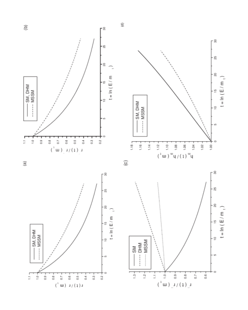
Figure 1: The scale dependence of the ratios: $r(t)/r(m_{t})$, $r^{\prime}(t)/r^{\prime}(m_{t})$, $r^{\prime\prime}(t)/r^{\prime\prime}(m_{t})$ and $h_{m}(t)/h_{m}(m_{t})$.

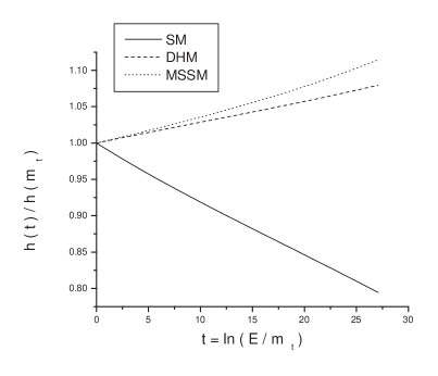
Figure 2: The scale dependence of the ratio $h(t)/h(m_{t})$.

IV Evolution of the observables

The solution of the renormalization group equations presented in Section III allows the analysis of the evolution of all the observables related with the Yukawa couplings and the Higgs vacuum expectation values, i.e. the quark masses and the Cabibbo-Kobayashi-Maskawa matrix. The results of this section have been obtained from the explicit solutions from the previous section. Their validity and precision are therefore the same, i.e. the terms of the order $\lambda^{4}$ and higher have been neglected. We start with the analysis of the quark masses presenting first the analytical results and then showing the corresponding graphs. The same type of the analysis will be also applied to the CKM matrix.

IV.1 Quark masses

The quark masses after the spontaneous symmetry breaking are equal to

$$m_{i}=\frac{{v}_{i}}{\sqrt{2}}Y_{i}$$ (31)

where $Y_{i}$ are the eigenvalues of the corresponding Yukawa couplings and ${v}_{i}$ is the vacuum expectation value of the Higgs field. For the theories with one Higgs doublet (SM) there is one Higgs vacuum expectation value and for two Higgs doublets (DHM, MSSM) there is one VEV for the up quarks and another for the down quarks.

IV.1.1 Up quark masses

The evolution of the eigenvalues $\left(Y_{u},Y_{c},Y_{t}\right)$ for the up quarks is given in Eqs. (14) and the evolution of the VEV’s is given in Eq. (29). Using Eq. (31) we thus obtain

$$m_{i}^{u}\left(t\right)=\frac{{v}_{u}(t)}{\sqrt{2}}Y_{i}^{u}(t)=\frac{{v}_{u}(t_{0})}{\sqrt{2}}Y_{i}^{u}(t_{0})\sqrt{r(t)r^{\prime\prime}_{{v}_{u}}(t)}h_{m}^{K_{i}^{u}}\left(t\right)=m_{i}^{u}(t_{0})\sqrt{r(t)r^{\prime\prime}_{{v}_{u}}(t)}h_{m}^{K_{i}^{u}}\left(t\right),$$ (32)

and the power $K_{i}^{u}$ is equal

$$K_{u,c}^{u}=\alpha_{3}^{u}+\alpha_{3}^{{v}_{u}},\,\,\,\,\,\,\,K_{t}^{u}=\alpha_{2}^{u}+\alpha_{3}^{u}+\alpha_{3}^{{v}_{u}}.$$ (33)

In Figs. 3 (a) and 3 (b) we show the running of the ratios of the up quark masses $m_{i}(t)/m_{i}(t_{0})$ $i=u,c,t$ for three models SM, DHM and MSSM.

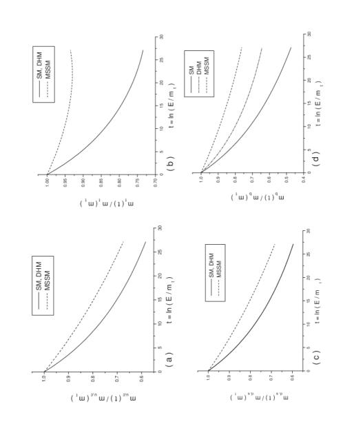
Figure 3: The scale dependence of the ratios $m_{i}(t)/m_{i}(m_{t})$ for the up and down quarks.

IV.1.2 Down quark masses

The evolution of the eigenvalues of the down quark Yukawa couplings is more complicated because the diagonalizing matrices are also running. If we write the matrix $y_{d}$ in the form

$$y_{d}=\left(U_{L}^{d}\right)^{\dagger}Y^{d}\left(U_{R}^{d}\right),$$ (34)

then Eq. (10) becomes

$$\frac{d\left(\left(U_{L}^{d}\right)^{\dagger}Y^{d}\left(U_{R}^{d}\right)\right)}{dt}=\frac{1}{(4\pi)^{2}}\left\{\alpha_{1}^{d}(t)+\alpha_{2}^{d}y_{u}^{\phantom{\dagger}}y_{u}^{\dagger}+\alpha_{3}^{d}\text{Tr}(y_{u}^{\phantom{\dagger}}y_{u}^{\dagger})\right\}\left(\left(U_{L}^{d}\right)^{\dagger}Y^{d}\left(U_{R}^{d}\right)\right),$$ (35)

which after some simple manipulations becomes

$$U_{L}^{d}\frac{d\left(U_{L}^{d}\right)^{\dagger}}{dt}Y^{d}+\frac{dY^{d}}{dt}+Y^{d}\frac{d\left(U_{R}^{d}\right)}{dt}\left(U_{R}^{d}\right)^{\dagger}=\frac{1}{(4\pi)^{2}}\left(U_{L}^{d}\right)\left\{\alpha_{1}^{d}(t)+\alpha_{2}^{d}y_{u}^{\phantom{\dagger}}y_{u}^{\dagger}+\alpha_{3}^{d}\text{Tr}(y_{u}^{\phantom{\dagger}}y_{u}^{\dagger})\right\}\left(U_{L}^{d}\right)^{\dagger}Y^{d}\equiv\frac{1}{(4\pi)^{2}}M^{{vv}}Y^{d},$$ (36)

$$M^{{vv}}\equiv\hat{V}^{\dagger}\left\{\alpha_{1}^{d}(t)+\alpha_{2}^{d}Y_{u}^{2}+\alpha_{3}^{d}\text{Tr}(Y_{u}^{2})\right\}\hat{V},$$ (37)

where the matrix $M^{{vv}}$ is introduced for notational simplicity.

The matrices $U_{L}^{d}\frac{d\left(U_{L}^{d}\right)^{\dagger}}{dt}$ and $\frac{d\left(U_{R}^{d}\right)}{dt}\left(U_{R}^{d}\right)^{\dagger}$ are antihermitian (this follows from unitarity) so their diagonal elements are purely imaginary. The diagonal elements of the matrix $Y_{d}$ are purely real and the matrix $M^{{vv}}$ is hermitian, so after taking the real part of the diagonal elements of Eq. (36) we obtain

$$\left(\frac{dY^{d}}{dt}\right)_{ii}=\frac{1}{(4\pi)^{2}}\left(M^{{vv}}Y^{d}\right)_{ii}.$$ (38)

The matrix $\left(M^{{vv}}\right)_{ij}$ has the simple form in our approximation.

$$\left(M^{{vv}}\right)_{ij}=\left(\hat{V}^{\dagger}\alpha_{1}^{d}(t)\hat{V}+\hat{V}^{\dagger}\alpha_{2}^{d}Y_{u}^{2}\hat{V}+\hat{V}^{\dagger}\alpha_{3}^{d}\text{Tr}(Y_{u}^{2})\hat{V}\right)_{ij}=\left\{\alpha_{1}^{d}(t)+\alpha_{3}^{d}Y_{t}^{2}\right\}\delta_{ij}+\alpha_{2}^{d}Y_{t}^{2}\hat{V}_{it}^{\dagger}\hat{V}_{tj}+{\cal O}(\lambda^{4}).$$ (39)

The last step in derivation of (39) follows from the approximation based on hierarchy

$$\left(Y^{u}\right)_{11}\thicksim\lambda^{7}Y_{t},\quad\quad\left(Y^{u}\right)_{22}\thicksim\lambda^{3.5}Y_{t}.$$

Finally we obtain the following equations for the eigenvalues of the down quark Yukawa couplings

$$\frac{dY_{ii}^{d}}{dt}=\frac{1}{(4\pi)^{2}}\left\{\alpha_{1}^{d}+\alpha_{2}^{d}Y_{t}^{2}\left|\hat{V}_{ti}\right|^{2}+\alpha_{3}^{d}Y_{t}^{2}\right\}Y_{ii}^{d}+{\cal O}(\lambda^{4}).$$ (40)

Using the hierarchical properties of the $\hat{V}$ matrix

$$\left|\hat{V}_{td}\right|^{2}\thicksim\lambda^{6},\,\,\,\,\,\,\,\,\,\,\,\left|\hat{V}_{ts}\right|^{2}\thicksim\lambda^{4},\,\,\,\,\,\,\,\,\left|\hat{V}_{tb}\right|^{2}=1,$$ (41)

we obtain the following equations for the eigenvalues of the down quarks Yukawa couplings

$$\begin{split}\frac{dY_{d,s}}{dt}&=\frac{1}{(4\pi)^{2}}\left\{\alpha_{1}^{d}+\alpha_{3}^{d}Y_{t}^{2}\right\}Y_{d,s}+{\cal O}(\lambda^{4}),\\ \frac{dY_{b}}{dt}&=\frac{1}{(4\pi)^{2}}\left\{\alpha_{1}^{d}+\left(\alpha_{3}^{d}+\alpha_{2}^{d}\right)Y_{t}^{2}\right\}Y_{b}+{\cal O}(\lambda^{4}).\end{split}$$ (42)

The solution of Eqs. (42) reads

$$\begin{split}Y_{d,s}(t)&=Y_{d,s}(t_{0})\sqrt{r^{\prime}(t)}h_{m}^{\alpha_{3}^{d}}(t),\\ Y_{b}(t)&=Y_{b}(t_{0})\sqrt{r^{\prime}(t)}\,h_{m}^{\left(\alpha_{2}^{d}+\alpha_{3}^{d}\right)}(t).\end{split}$$ (43)

where the function $r^{\prime}(t)$ is given in Eq. (22). These results complement previous results shown in Sec. III. Now, Eqs. (43) together with the VEV evolution Eq. (29) gives the evolution of the down quark masses

$$m_{i}^{d}(t)=\frac{{v}_{d}(t)}{\sqrt{2}}Y_{i}^{d}(t)=\frac{{v}_{d}(t_{0})}{\sqrt{2}}Y_{i}^{d}(t_{0})\sqrt{r^{\prime}(t)r^{\prime\prime}_{{v}_{d}}(t)}h_{m}^{K_{i}^{d}}\left(t\right)=m_{i}^{d}(t_{0})\sqrt{r^{\prime}(t)r^{\prime\prime}_{{v}_{d}}(t)}h_{m}^{K_{i}^{d}}\left(t\right)$$ (44)

there the powers $K_{i}^{d}$ are equal to

$$K_{d,s}^{d}=\alpha_{3}^{d}+\alpha_{3}^{{v}_{d}},\,\,\,\,\,\,\,K_{b}^{d}=\alpha_{2}^{d}+\alpha_{3}^{d}+\alpha_{3}^{{v}_{d}}.$$ (45)

Eqs. (44) give the analytical form of the down quark mass evolution. The evolution of the ratios of the down quark masses for three models SM, DHM, and MSSM is shown in Fig. 3 (c) and Fig. 3 (d).

IV.2 Cabibbo-Kobayashi-Maskawa matrix

The other set of observables is related with the CKM matrix. These observables include the absolute values of the matrix elements of the CKM matrix, Jarlskog’s parameter $J$ n12a , Wolfenstein parameters $\lambda$, $A$, $\rho$, $\eta$ W ; Buras2 and the angles of the unitarity triangle n12 ; Buras3 .

The evolution of the CKM matrix is simpler than that for masses because the CKM matrix depends only on the left diagonalizing matrices of the biunitary transformations for the Yukawa couplings and as was shown in Ref. ref0 the evolution of CKM matrix depends only on one function of the energy $h(t)$. This fact implies that there exist correlations between the evolution of the various elements of the CKM matrix.

In the following we shall first find the evolution equations of the absolute values of the CKM matrix elements and afterwards analyze the $J$ parameter and the unitarity triangle.

IV.2.1 Evolution of the absolute values of the CKM matrix $\hat{V}$.

Our starting point is Eq. (36). We take now the imaginary part of the diagonal elements and the full off-diagonal elements of Eq. (36), and using the form of the matrix $M^{{vv}}$ in Eq. (39) we obtain

$$\left(\left(U_{L}^{d}\right)\frac{d\left(U_{L}^{d}\right)^{\dagger}}{dt}\right)_{ii}+\left(\frac{d\left(U_{R}^{d}\right)}{dt}\left(U_{R}^{d}\right)^{\dagger}\right)_{ii}=0$$ (46)

and

$$\left(\left(U_{L}^{d}\right)\frac{d\left(U_{L}^{d}\right)^{\dagger}}{dt}\right)_{ij}Y_{j}^{d}+Y_{i}^{d}\left(\frac{d\left(U_{R}^{d}\right)}{dt}\left(U_{R}^{d}\right)^{\dagger}\right)_{ij}=\frac{1}{(4\pi)^{2}}\alpha_{2}^{d}Y_{t}^{2}\hat{V}_{ti}^{*}\hat{V}_{tj}Y_{j}^{d},\;\;\;\;\;\;i\neq j.$$ (47)

The hermitian conjugate of Eq. (47) reads

$$Y_{i}^{d}\left(\left(U_{L}^{d}\right)\frac{d\left(U_{L}^{d}\right)^{\dagger}}{dt}\right)_{ij}+\left(\frac{d\left(U_{R}^{d}\right)}{dt}\left(U_{R}^{d}\right)^{\dagger}\right)_{ij}Y_{j}^{d}=-\frac{1}{(4\pi)^{2}}\alpha_{2}^{d}Y_{t}^{2}Y_{i}^{d}\hat{V}_{ti}^{*}\hat{V}_{tj},\,\,\,\,\,\,\,\,\,\,\,\,\,\,\,\,\,\,\,\,\,\,\,i\neq j.$$ (48)

Now multiplying Eq. (47) by $Y_{i}^{d}\,$ and Eq. (48) by $Y_{j}^{d}\,$ and summing these equations, we obtain after some simple manipulations the differential equation for the evolution of the right diagonalizing matrix of the down sector

$$\left(\frac{d\left(U_{R}^{d}\right)}{dt}\left(U_{R}^{d}\right)^{\dagger}\right)_{ij}=-\frac{2Y_{i}^{d}Y_{j}^{d}}{\left(Y_{j}^{d}\right)^{2}+\left(Y_{i}^{d}\right)^{2}}\left(\left(U_{L}^{d}\right)\frac{d\left(U_{L}^{d}\right)^{\dagger}}{dt}\right)_{ij}.$$ (49)

Eq. (49) gives the relation between the evolution of the left and right diagonalizing matrices and it is the key relation that permits the derivation of the evolution of the left diagonalizing matrix of the down quark Yukawa couplings. Inserting Eq. (49) in Eq. (47) we obtain the evolution equation for the $U_{L}^{d}$ matrix

$$\frac{\left(Y_{j}^{d}\right)^{2}-\left(Y_{i}^{d}\right)^{2}}{\left(Y_{j}^{d}\right)^{2}+\left(Y_{i}^{d}\right)^{2}}\left(U_{L}^{d}\frac{d\left(U_{L}^{d}\right)^{\dagger}}{dt}\right)_{ij}=\frac{1}{(4\pi)^{2}}\alpha_{2}^{d}Y_{t}^{2}\hat{V}_{ti}^{*}\hat{V}_{tj}\,\,\,\,\,\,\,\,\,\,\,\,\,\,\,\,\,\,\,\,\,i\neq j.$$ (50)

We will now convert Eq. (50) into equations for the CKM matrix elements. To this end we first notice that within our approximation (neglecting all terms of the order $\lambda^{4}$ and higher)

$$\frac{\left(Y_{j}^{d}\right)^{2}-\left(Y_{i}^{d}\right)^{2}}{\left(Y_{j}^{d}\right)^{2}+\left(Y_{i}^{d}\right)^{2}}=-\text{sign}(i-j)+{\cal O}(\lambda^{4}),$$ (51)

where $\text{sign}(i-j)=\mp 1$ for $i\lessgtr j$.

Next we know that the up quark diagonalizing matrix $U_{L}^{u}$ does not depend on the energy. Using the definition of the CKM matrix $\hat{V}=U_{L}^{u}\left(U_{L}^{d}\right)^{\dagger}$ we obtain

$$\hat{V}^{\dagger}\frac{d\hat{V}}{dt}=\left(U_{L}^{d}\right)\left(U_{L}^{u}\right)^{\dagger}U_{L}^{u}\frac{d\left(U_{L}^{d}\right)^{\dagger}}{dt}=\left(U_{L}^{d}\right)\frac{d\left(U_{L}^{d}\right)^{\dagger}}{dt}.$$ (52)

Now from Eqs. (50), (51) and (52) the following equations are obtained

$$\left(\hat{V}^{\dagger}\frac{d\hat{V}}{dt}\right)_{ij}=-\frac{1}{(4\pi)^{2}}\text{sign}(i-j)\alpha_{2}^{d}Y_{t}^{2}\hat{V}_{ti}^{*}\hat{V}_{tj}.$$ (53)

Eq. (53) is valid only for $i\neq j$ but from the property that the matrix $\left(\hat{V}^{\dagger}d\hat{V}/dt\right)$ is antiunitary and its diagonal elements are purely imaginary, we obtain equations for the absolute value of the elements of the CKM matrix

$$\frac{1}{\left|\hat{V}_{cd}\right|^{2}}\frac{d\left|\hat{V}_{cd}\right|^{2}}{dt} = \frac{2}{(4\pi)^{2}}\alpha_{2}^{d}Y_{t}^{2}\left|\hat{V}_{td}\right|^{2},$$ (54a)

$$\frac{1}{\left|\hat{V}_{td}\right|^{2}}\frac{d\left|\hat{V}_{td}\right|^{2}}{dt} = -\frac{2}{(4\pi)^{2}}\alpha_{2}^{d}Y_{t}^{2}\left(1-\left|\hat{V}_{td}\right|^{2}\right),$$ (54b)

$$\frac{1}{\left|\hat{V}_{ub}\right|^{2}}\frac{d\left|\hat{V}_{ub}\right|^{2}}{dt} = -\frac{2}{(4\pi)^{2}}\alpha_{2}^{d}Y_{t}^{2}\left|\hat{V}_{tb}\right|^{2},$$ (54c)

$$\frac{1}{\left|\hat{V}_{cb}\right|^{2}}\frac{d\left|\hat{V}_{cb}\right|^{2}}{dt} = -\frac{2}{(4\pi)^{2}}\alpha_{2}^{d}Y_{t}^{2}\left|\hat{V}_{tb}\right|^{2},$$ (54d)

and from the unitarity of the CKM matrix we obtain the evolution of the remaining CKM matrix elements.

To solve Eqs. (54) let us notice the following relation

$$\frac{2}{(4\pi)^{2}}\alpha_{2}^{d}Y_{t}^{2}=\frac{1}{h^{2}}\frac{dh^{2}}{dt},$$ (55)

where $h\left(t\right)\equiv\left[h_{m}(t)\right]^{\alpha_{2}^{d}}$ and $h_{m}(t)$ is the function introduced in Eq. (16). Using relation (55) we obtain from Eq. (54b)

$$|\hat{V}_{td}\left(t\right)|^{2}=\frac{|\hat{V}_{td}^{0}|^{2}}{h^{2}+\left(1-h^{2}\right)|\hat{V}_{td}^{0}|^{2}},\;\;\;\;\;\;\;\text{where}\,\,\,\,\hat{V}_{ij}^{0}\equiv\hat{V}_{ij}\left(t_{0}\right).$$ (56a)

From Eqs. (54a) and  (54b) we obtain

$$|\hat{V}_{cd}\left(t\right)|^{2}=\frac{h^{2}|\hat{V}_{cd}^{0}|^{2}}{h^{2}+(1-h^{2})|\hat{V}_{td}^{0}|^{2}}.$$ (56b)

Using the relation $$1-|\hat{V}_{tb}|^{2}=|\hat{V}_{ub}|^{2}+|\hat{V}_{cb}|^{2}$$ we derive from of Eqs. (54c) and (54d) the following result

$$|\hat{V}_{tb}(t)|^{2}=\frac{h^{2}|\hat{V}_{tb}^{0}|^{2}}{1+(h^{2}-1)|\hat{V}_{tb}^{0}|^{2}}.$$ (56c)

and this result yields with the help of Eqs. (54c) and (54d ) the evolution of the $$|\hat{V}_{ub}(t)|^{2} |\hat{V}_{cb}(t)|^{2}$$ and :

$$|\hat{V}_{ub}\left(t\right)|^{2}=\frac{|\hat{V}_{ub}^{0}|^{2}}{1+(h^{2}-1)|\hat{V}_{tb}^{0}|^{2}},$$ (56d)

$$\left|\hat{V}_{cb}\left(t\right)\right|^{2}=\frac{\left|\hat{V}_{cb}^{0}\right|^{2}}{1+\left(h^{2}-1\right)|\hat{V}_{tb}^{0}|^{2}}.$$ (56e)

The remaining elements of the CKM matrix are obtained from the unitarity relation

$$\left|\hat{V}_{ud}\left(t\right)\right|^{2}=\frac{h^{2}\left|\hat{V}_{ud}^{0}\right|^{2}}{h^{2}+\left(1-h^{2}\right)\left|\hat{V}_{td}^{0}\right|^{2}},$$ (56f)

$$\left|\hat{V}_{us}\left(t\right)\right|^{2}=\left|\hat{V}_{us}^{0}\right|^{2}+\left(h^{2}-1\right)\left[\frac{|\hat{V}_{ub}^{0}|^{2}|\hat{V}_{tb}^{0}|^{2}}{1+\left(h^{2}-1\right)|\hat{V}_{tb}^{0}|^{2}}-\frac{|\hat{V}_{ud}^{0}|^{2}|\hat{V}_{td}^{0}|^{2}}{h^{2}+\left(1-h^{2}\right)|\hat{V}_{td}^{0}|^{2}}\right],$$ (56g)

$$\left|\hat{V}_{cs}\left(t\right)\right|^{2}=\left|\hat{V}_{cs}^{0}\right|^{2}+\left(h^{2}-1\right)\left[\frac{|\hat{V}_{cb}^{0}|^{2}|\hat{V}_{tb}^{0}|^{2}}{1+\left(h^{2}-1\right)|\hat{V}_{tb}^{0}|^{2}}-\frac{|\hat{V}_{cd}^{0}|^{2}|\hat{V}_{td}^{0}|^{2}}{h^{2}+\left(1-h^{2}\right)|\hat{V}_{td}^{0}|^{2}}\right],$$ (56h)

$$\left|\hat{V}_{ts}\left(t\right)\right|^{2}=\left|\hat{V}_{ts}^{0}\right|^{2}-\left(h^{2}-1\right)\left[\frac{|\hat{V}_{tb}^{0}|^{2}(1-|\hat{V}_{tb}^{0}|^{2})}{1+\left(h^{2}-1\right)|\hat{V}_{tb}^{0}|^{2}}-\frac{|\hat{V}_{td}^{0}|^{2}(1-|\hat{V}_{td}^{0}|^{2})}{h^{2}+\left(1-h^{2}\right)|\hat{V}_{td}^{0}|^{2}}\right].$$ (56i)

Eqs. (56) represent the RG evolution of the CKM matrix. The absolute values of the CKM matrix elements do not depend on the parameterization of the CKM matrix. Notice that in agreement with the Theorem 1 in Ref. ref0 the evolution of the CKM matrix depends only on one function $h(t)$ of energy. It is for this reason that we consider $h(t)$ as an universal function of energy.

IV.2.2 Jarlskog Invariant

Jarlskog parameter $J$ is defined as n12a

$$J=\Im\left[\hat{V}_{ud}\hat{V}_{cs}\hat{V}_{us}^{*}\hat{V}_{cd}^{*}\right]=\Im\left[\hat{V}_{ud}\hat{V}_{tb}\hat{V}_{ub}^{*}\hat{V}_{td}^{*}\right]=\Im\left(D\right),$$ (57)

and it is nonvanishing if the CKM matrix is non CP invariant.

Let us now consider the following expression

$$\frac{d\ln D}{dt}=\frac{d\ln\left(\hat{V}_{ud}\hat{V}_{tb}\hat{V}_{ub}^{*}\hat{V}_{td}^{*}\right)}{dt}=\frac{1}{\hat{V}_{ud}}\frac{d}{dt}\hat{V}_{ud}+\frac{1}{\hat{V}_{tb}}\frac{d}{dt}\hat{V}_{tb}+\frac{1}{\hat{V}_{ub}^{*}}\frac{d}{dt}\hat{V}_{ub}^{*}+\frac{1}{\hat{V}_{td}^{*}}\frac{d}{dt}\hat{V}_{td}^{*}.$$ (58)

Now using Eq. (53) and the property that the matrix $\hat{V}^{\dagger}\frac{d\hat{V}}{dt}$ is antihermitian (and has imaginary diagonal elements) we obtain

$$\frac{d\ln D}{dt}=-2\alpha_{2}^{d}Y_{t}^{2}\left(\left|\hat{V}_{tb}\right|^{2}-\left|\hat{V}_{td}\right|^{2}\right)\approx-2\alpha_{2}^{d}Y_{t}^{2}\left|\hat{V}_{tb}\right|^{2},$$ (59)

and thus the Jarlskog invariant fulfills the equation

$$\frac{d\ln J}{dt}=-2\alpha_{2}^{d}Y_{t}^{2}\left|\hat{V}_{tb}\right|^{2}=-\frac{1}{h^{2}}\frac{dh^{2}}{dt}\left|\hat{V}_{tb}\right|^{2}$$ (60)

which gives using Eq. (56c)

$$\ln\frac{J}{J_{0}}=\ln\frac{1}{\left|1+(h^{2}-1)|\hat{V}_{tb}^{0}|^{2}\right|}$$ (61)

or

$$J=\frac{J_{0}}{\left|1+(h^{2}-1)|\hat{V}_{tb}^{0}|^{2}\right|}\approx\frac{J_{0}}{h^{2}}.$$ (62)

The evolution of the Jarlskog invariant is given in Fig. 4.

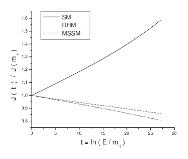
Figure 4: The scale dependence of the ratio $J(t)/J(m_{t})$ for the Jarlskog invariant.

IV.2.3 The Wolfenstein Parameters

Eqs. (56) can be written in an approximate form using the hierarchy of the CKM matrix, given by the Wolfenstein parameterization W ; Buras2

$$\hat{V}=\left(\begin{array}[]{ccc}1-\frac{1}{2}\lambda^{2}&\lambda&A\lambda^{3}(\rho-i\eta)\\ -\lambda&1-\frac{1}{2}\lambda^{2}&A\lambda^{2}\\ A\lambda^{3}(1-\bar{\rho}-i\bar{\eta})&-A\lambda^{2}&1\end{array}\right),\;\;\;\bar{\rho}=\rho\left(1-\frac{\lambda^{2}}{2}\right),\;\;\;\bar{\eta}=\eta\left(1-\frac{\lambda^{2}}{2}\right).$$ (63)

Now neglecting all the terms of the relative order $\lambda^{4}$ and higher, we obtain

$$\displaystyle 1-\left|\hat{V}_{ud}\right|^{2}\approx 1-\left|\hat{V}_{ud}^{0}\right|^{2},\;\;\;\;\;\left|\hat{V}_{us}\right|^{2}\approx\left|\hat{V}_{us}^{0}\right|^{2},\;\;\;\;\;\left|\hat{V}_{ub}\right|^{2}\approx\frac{\left|\hat{V}_{ub}^{0}\right|^{2}}{h^{2}}$$

$$\displaystyle\left|\hat{V}_{cd}\right|^{2}\approx\left|\hat{V}_{cd}^{0}\right|^{2},\;\;\;\;\;1-\left|\hat{V}_{cs}\right|^{2}\approx 1-\left|\hat{V}_{cs}^{0}\right|^{2}+\frac{1-h^{2}}{h^{2}}\left|\hat{V}_{cb}^{0}\right|^{2},\;\;\;\;\;\left|\hat{V}_{cb}\right|^{2}\approx\frac{\left|\hat{V}_{cb}^{0}\right|^{2}}{h^{2}},$$ (64)

$$\displaystyle\left|\hat{V}_{td}\right|^{2}\approx\frac{\left|\hat{V}_{td}^{0}\right|^{2}}{h^{2}},\;\;\;\;\;\left|\hat{V}_{ts}\right|^{2}\approx\frac{\left|\hat{V}_{ts}^{0}\right|^{2}}{h^{2}},\;\;\;\;\;1-\left|\hat{V}_{tb}\right|^{2}\approx\frac{1-\left|\hat{V}_{tb}^{0}\right|^{2}}{h^{2}}.$$

From Eqs. (64) immediately follows the simple evolution of the Wolfenstein parameters

$$A\left(t\right)=\frac{A}{h(t)},\,\,\,\,\,\,\,\,\,\,\text{and\thinspace\thinspace\thinspace\thinspace\thinspace\thinspace\thinspace}\lambda,\rho,\eta\text{ are invariant.}$$ (65)

Notice that the dependence of the CKM matrix and Wolfenstein parameters on the renormalization scheme is given in Ref. kniehl .

IV.2.4 The Unitarity triangle

The unitarity triangle n12 ; Buras3 is obtained from the scalar product of the first column of the $\hat{V}$ matrix by the complex conjugate of the third

$$\hat{V}_{ud}\hat{V}_{ub}^{*}+\hat{V}_{cd}\hat{V}_{cb}^{*}+\hat{V}_{td}\hat{V}_{tb}^{*}=0$$ (66)

and then by rescaling it in such a way that the lengths of the sides of the resulting triangle are equal

$$R_{b}=(1-\frac{\lambda^{2}}{2})\frac{1}{\lambda}\left|\frac{\hat{V}_{ub}}{\hat{V}_{cb}}\right|,\;\;\;\;\;R_{t}=\frac{1}{\lambda}\left|\frac{\hat{V}_{td}}{\hat{V}_{cb}}\right|,\;\;\;\;\;1.$$ (67)

From Eqs. (64) and (65) it immediately follows that $R_{b}$ and $R_{t}$ are invariant upon the evolution which implies that the unitarity triangle is also invariant. Thus the complex phases of the CKM matrix elements $\hat{V}_{td}$ and $\hat{V}_{ub}$ (angles $\beta$ and $\gamma$) are also invariant up to the order $\lambda^{4}$.

V Conclusions

In this paper we analyzed the solutions of the RGE for the quark Yukawa couplings, for the Higgs VEV’s and also the evolution of all the observables that follow from them. The results depend on the model dependent functions given in Eq. (30). The most interesting is the universal function $h(t)$ because only on this function depends the evolution of the CKM matrix, Eq. (56) or (64). The running of the absolute values of the CKM matrix elements and the invariance of the unitarity triangle angles implies that the evolution of the CKM matrix is remarkably simple

$$\left(\begin{array}[]{ccc}\displaystyle\hat{V}_{ud}^{0}&\displaystyle\hat{V}_{ud}^{0}&\displaystyle\hat{V}_{ub}^{0}\\ \displaystyle\hat{V}_{cd}^{0}&\displaystyle\hat{V}_{cs}^{0}&\displaystyle\hat{V}_{cb}^{0}\\ \displaystyle\hat{V}_{td}^{0}&\displaystyle\hat{V}_{ts}^{0}&\displaystyle\hat{V}_{tb}^{0}\end{array}\right)\longrightarrow\left(\begin{array}[]{ccc}\displaystyle\hat{V}_{ud}^{0}&\displaystyle\hat{V}_{ud}^{0}&\displaystyle\frac{\hat{V}_{ub}^{0}}{h}\\ \displaystyle\hat{V}_{cd}^{0}&\displaystyle\hat{V}_{cs}^{0}&\displaystyle\frac{\hat{V}_{cb}^{0}}{h}\\ \displaystyle\frac{\hat{V}_{td}^{0}}{h}&\displaystyle\frac{\hat{V}_{ts}^{0}}{h}&\displaystyle\hat{V}_{tb}^{0}\end{array}\right)$$ (68)

We observe (see Fig. 2) that the function $h(t)$ is decreasing for the SM and increasing for the DHM and MSSM. This results in a qualitatively different evolution of the matrix elements and the observables related to the CKM matrix for the SM in comparison to the DHM and MSSM. An important result is the dependence on it of the Jarlskog invariant which is shown in Fig. 4. We thus see that the CP violation is enhanced with increasing energy in the SM while it decreases for the DHM and MSSM.

The evolution of the unitarity triangle is also very important. We have shown that the angles of the unitarity triangle remain constant upon the evolution. The invariance of the angles of the unitarity triangle is very significant because it means that at the grand unification scale the angles are the same as at the low energy so if there is a symmetry at the grand unification scale then it has to predict the low energy angles of the unitarity triangle. This strongly constrains the possible symmetries or textures at the grand unification scale.

As we discussed in Section I our results are approximate and we kept the terms up to the order $\lambda^{3}$. In the next order one has to keep the powers up to the order $\lambda^{4}$. In this approximation the results are qualitatively the same and the only corrections are small modifications of the functions $h_{m}(t)$ and $h(t)$. The next order, $\lambda^{5}$, is significantly different and it will be discussed elsewhere.

References

• (1) R.D. Peccei and K. Wang, Phys. Rev. D53, 2712 (1996); H. González et al., Phys. Lett. B 440, 94 (1998); H. González et al., A New symmetry of Quark Yukawa Couplings, page 755, International Europhysics Conference on High Energy Physics, Jerusalem 1997, eds. Daniel Lellouch, Giora Mikenberg, Eliezer Rabinovici, Springer-Verlag 1999.
• (2) K.S. Babu, Z. Phys.  C 35, 69 (1987); P. Binetruy and P. Ramond, Phys. Lett.  B350, 49 (1995); K. Wang, Phys. Rev. D54, 5750 (1996).
• (3) B. Grzadkowski and M. Lindner, Phys. Lett.  B193, 71 (1987); B. Grzadkowski, M. Lindner and S. Theisen, Phys. Lett. B198, 64 (1987); M. Olechowski and S. Pokorski, Phys. Lett.  B 257, 388 (1991); G. Cvetic, C.S. Kim and S.S. Hwang, Int. J. Mod. Phys.  A14 769 (1999).M.E. Machacek and M.T. Vaughn, Nucl. Phys.  B222, 83 (1983); B236, 221 (1984); B249, 70 (1985); C. Balzereit, Th. Hansmann, T. Mannel and B. Plümper, Eur. Phys. J. C9 197 (1999), hep-ph/9810350.
• (4) H. Arason, et al, Phys. Rev.  D46, 3945 (1992); H. Arason, et al, Phys. Rev.  D47, 232 (1992); D.J. Castaño, E.J. Piard and P. Ramond, Phys. Rev.  D49, 4882 (1994).
• (5) H. Fusaoka and Y. Koide, Phys. Rev.  D57, 3986 (1998).
• (6) K. Sasaki, Z. Phys.  C 32, 149 (1986).
• (7) S.R. Juárez W., S.F. Herrera, P. Kielanowski and G. Mora, Energy dependence of the quark masses and mixings in Particles and Fields, Ninth Mexican School, Metepec, Puebla, México. AIP Conference Proceedings 562 (2001) 303-308, ISBN 1-56396-998-X, ISSN 0094-243X, hep-ph/0009148.
• (8) N. Nimai Singh, Eur. Phys. J. C19, 137 (2001), hep-ph/0009211.
• (9) Yoshio Koide, Hideo Fusaoka, Phys. Rev. D64, 053014 (2001), hep-ph/0011070.
• (10) C.R. Das, M.K. Parida, Eur. Phys.J. C20, 121 (2001). hep-ph/0010004.
• (11) Cheng-Wei Chiang, Phys. Rev. D63, 076009 (2001), hep-ph/0011195.
• (12) N. Cabibbo, Phys. Rev. Lett. 10, 531 (1963).
• (13) M. Kobayashi, T. Maskawa, Prog. Theor. Phys. 49, 652 (1973).
• (14) P. Kielanowski, S.R. Juárez W. and G. Mora, Phys. Lett. B479, 181 (2000). S. R. Juárez W., P. Kielanowski and G. Mora, New Properties of the Renormalization Group Equations of the Yukawa Couplings and CKM Matrix in the Proceedings of the Eighth Mexican School Particles and Fields, Oaxaca, México. AIP Conference Proceedings 490 (1998), 351-354, ed. J.C. D’Olivo, G. López C. and M. Mondragón, L.C. Catalog Card No. 99-067150, ISBN 1-56396-895-9, ISSN 0094-243X., DOE CONF-981188.
• (15) Notice that in Ref. ref0 we used a slightly unfortunate notation by denoting the eigenvalues of the QYC matrices by the symbol $m_{i}$ which coincided with the notation for the quark masses. In this paper we use the symbol $Y_{i}$ for the eigenvalues of the QYC matrices and $m_{i}$ for the quark masses.
• (16) K. Hagiwara et al., Phys. Rev. D66, 010001 (2002).
• (17) C. Jarlskog, Phys. Rev. Lett.  55 1039 (1985) and Zeit. f. Phys. C29, 491 (1985).
• (18) L. Wolfenstein, Phys. Rev. Lett. 51, 1945 (1983).
• (19) A.J. Buras, M.E. Lautenbacher and G. Ostermaier, Phys. Rev. D 50, 3433 (1994).
• (20) B.A. Kniehl, F. Madricardo and M. Steinhauser, Phys. Rev. D 62, 073010 (2000).
• (21) C. Jarlskog and R. Stora, Phys. Lett.  B208, 268 (1988); L.-L. Chau and W.-Y. Keung, Phys. Rev. Lett. 53, 1802 (1984).
• (22) Andrzej J. Buras, Flavour Physics and CP Violation in the SM, Introductory Lecture given at KAON 2001, Pisa, 12 June–17 June, 2001, hep-ph/0109197.