Abstract

We demonstrate that the dipole-hadron cross-section computed from the non-linear evolution equation for the Colour Glass Condensate saturates the Froissart bound in the case of a fixed coupling and for a small dipole ($Q^{2}\gg\Lambda_{QCD}^{2}$). That is, the cross-section increases as the logarithm squared of the energy, with a proportionality coefficient involving the pion mass and the BFKL intercept $(\alpha_{s}N_{c}/\pi)4\ln 2$. The pion mass enters via the non-perturbative initial conditions at low energy. The BFKL equation emerges as a limit of the non-linear evolution equation valid in the tail of the hadron wavefunction. We provide a physical picture for the transverse expansion of the hadron with increasing energy, and emphasize the importance of the colour correlations among the saturated gluons in suppressing non-unitary contributions due to long-range Coulomb tails. We present the first calculation of the saturation scale including the impact parameter dependence. We show that the cross-section at high energy exhibits geometric scaling with a different scaling variable as compared to the intermediate energy regime.

1 Introduction

One of the striking features of the physics of strong interaction is that at high energies, cross sections are slowly, but monotonously, increasing with $s$ ($=$ the total center-of-mass energy squared). For instance, the data for the $pp$ and $p\bar{p}$ total cross sections at high energy can be reasonably well fitted by both $s^{\delta}$ (with $\delta\approx 0.09$) and $\ln^{2}s$, although the $\ln^{2}s$ growth appears to be favored by recent investigations [1].

At a theoretical level, it was proven many years ago that in the limit $s\to\infty$, the hadronic total cross sections must rise no faster than $(\pi/m_{\pi}^{2})\ln^{2}s$ [2, 3, 4]. This is the Froissart bound, which is a consequence of very general principles, such as unitarity, crossing and analiticity, but does not rely on any detailed dynamical information. So, in reality, this bound may very well be not saturated, although the measured cross-sections seem to do so (at least, in so far as they are consistent with a squared log dependence upon the energy). In fact, a simple, qualitative mechanism realising this $\ln^{2}s$ growth has been proposed by Heisenberg [5] already before Froissart bound has been rigorously proven (a similar argument is briefly discussed by Froissart [2]). However, we are not aware of any field-theoretical implementation of this, or other, argument. (See also Ref. [6] for a recent review and more references, and Ref. [1] for a recent analysis of the data.)

The goal of this paper is to see how the Froissart bound can be consistent with modern pictures of high energy strong interactions. To keep the discussion as simple as possible while still encompassing the interesting physics, we shall consider the scattering of a colour dipole off a hadronic target at very high energy. The “colour dipole” may be thought of as a quark-antiquark pair in a colourless state, like a quarkonium, or a fluctuation of the virtual photon in deep inelastic scattering. More generally, arbitrary hadronic probes can be considered as collections of “colour dipoles” at least in the approximation in which the number of colours $N_{c}$ is large (so that a gluon excitation can be effectively replaced by a $q\bar{q}$ pair). For our approximations to be justified, we shall assume that the dipole is “small”, in the sense that it has a small transverse size, $r_{\perp}\ll 1/\Lambda_{QCD}$, or a large transverse resolution: $Q^{2}\equiv 1/r_{\perp}^{2}\gg\Lambda_{QCD}^{2}$.

On the particular example of the dipole-hadron scattering, we shall develop an argument involving both perturbative and non-perturbative features of QCD, like non-linear quantum evolution, parton saturation, and confinement, which will lead us to the conclusion that the total cross-section respects, and even saturates, the Froissart bound (at least, in the case of a fixed coupling, that we shall exclusively consider in this paper). In its essence, our argument may be viewed as a modern version of Heisenberg’s original mechanism. But our main point is to place this mechanism within the context of our present theoretical understanding, and clarify to which extent perturbation theory may play a role in determining this result. In brief, we shall demonstrate that this mechanism is naturally realized by the solutions to non-linear evolution equations derived within perturbation theory, in Refs. [7, 8, 9, 10], but with non-perturbative initial conditions at low energy. In particular, our analysis will confirm, clarify and extend the conclusions reached in an early study [11] based on the GLR equation [12, 13], which is a simplified version of the non-linear evolution equations that we shall use in this paper.

The fact that perturbation theory is the appropriate tool to describe the high energy behaviour of hadronic cross-sections is by itself non-trivial, and deserves some comment. The first, and most certainly true, objection to the use of weak coupling methods comes from the fact that the Froissart bound involves the pion mass, and this surely must arise from confinement. And, indeed, this is how the pion mass enters also our calculations: via the non-perturbative initial condition that we shall assume, and which specifies the impact parameter dependence of the dipole-hadron scattering amplitude at low energy. But starting with this initial condition, we shall then study its evolution with increasing energy within perturbation theory, and show that the resulting cross-section saturates the Froissart bound at high energy.

The adequacy of perturbation theory even for such a limited purpose — the study of the quantum evolution of the cross-section with $s$ — is still non-trivial [6], and has been in fact disputed in recent papers [14]. It is first of all clear that ordinary perturbation theory, in the form of the BFKL equation [15] — which resums the dominant radiative corrections at high energy, but neglects the non-linear effects associated with high parton densities —, fails to describe the asymptotic behaviour at high energy: The BFKL equation predicts a power-law growth for the total cross section: $\sigma\sim{s}^{\omega\bar{\alpha}_{s}}$, with $\omega=4\ln 2$ and $\bar{\alpha}_{s}=\alpha_{s}N_{c}/\pi$, which clearly violates the Froissart bound. Besides, with increasing energy, the solution to the BFKL equation “diffuses” towards smaller and smaller transverse momenta, thus making the applicability of perturbation theory questionable.

But the objections in Ref. [14] actually apply to the more recently derived non-linear evolution equations [7, 8, 9, 10], in which non-linear effects cure the obvious pathologies of the BFKL equation. (Alternative derivations of some of these equations, at least in specific limits, have been given in Refs. [12, 13, 16, 17]. See also Refs. [18, 19] for recent reviews and more references.) Specifically, the non-linear effects associated with the high density of gluons in the hadron light-cone wavefunction (the “Colour Glass Condensate” [10]) lead to gluon saturation [12, 20, 21, 22], with important consequences for the high-energy scattering: First, this introduces a hard intrinsic momentum scale, the “saturation scale”, which is a measure of the density of the saturated gluons in the impact parameter space, and grows like a power of the energy. This limits the infrared diffusion [23] and thus provides a better justification for using weak coupling methods at high energy. Second, this ensures the unitarization of the dipole-hadron scattering amplitude at fixed impact parameter [24, 25, 26, 27, 8]. That is, with increasing energy, the hadron eventually turns “black” (i.e., the dipole is completely absorbed, or the scattering amplitude reaches the unitarity limit) at any given point $b_{\perp}$ in the impact parameter space.

However, by itself, the unitarization at given $b_{\perp}$ is not enough to guarantee the Froissart bound for the total cross-section, which involves an integration over all the impact parameters. Indeed, as a quantum mechanical object, the hadron has not a sharp edge, but rather a diffuse tail, so, with increasing energy, the “black disk” can extend to larger and larger impact parameters. The radial expansion of the black disk is controlled by the scattering in the surrounding “grey area”, where the gluon density is relatively low and the BFKL equation still applies. Given the problems of the BFKL equation alluded to before, it is not a priori clear whether this expansion is slow enough to ensure that the Froissart bound is respected. This would require a black disk radius which increases at most logarithmically with $s$. In Heisenberg’s original argument (but using the current terminology), such a logarithmic increase was ensured by a compensation between the power-law increase of the scattering amplitude with $s$ and its exponential decrease with $b\equiv|b_{\perp}|$. Such an exponential fall-off at large impact parameters is, of course, a true property of full QCD, and also the crucial assumption about our initial condition, but it is not clear whether this property can be preserved by the perturbative quantum evolution, which involves massless gluons and therefore long range interactions.

In fact, it was the main point of Ref. [14] to argue that the Coulomb tails associated with the saturated gluons should replace the exponential fall-off with $b\equiv|b_{\perp}|$ of the initial distribution by just a power-law fall-off, which would be then too slow to ensure the Froissart bound: the corresponding black disk radius would increase as a power of $s$.

However, as we shall explain in this paper, the argument in Ref. [14] is irrelevant for the problem at hand, and also incorrect in its original formulation. Part of the confusion in Ref. [14] comes from non-recognizing that the saturated gluons are actually colour neutral over a relatively short distance (of the order of the inverse saturation scale) [22, 18], and thus cannot produce Coulomb tails at large distances. Rather, the colour field produced by the saturated gluons is merely a dipolar field, whose fall-off with $b$ is sufficiently fast to respect the Froissart bound for the scattering of an external dipole. (In Ref. [14], this was masked by the fact that the authors were truly computing the scattering of a coloured external probe, although their verbal arguments were formally developed for a “dipole”.) As we shall see, for the relevant impact parameters, this long-range dipole-dipole scattering is subleading at high energy as compared to the short-range scattering off the local sources.

More precisely, we shall demonstrate that the region which controls the evolution of the cross section is the “grey area” outside, but close to the black disk. In this area, we expect perturbation theory to apply, since the local saturation scale is much larger than $\Lambda_{QCD}$. For an incoming dipole in this area, the dominant interactions are those with the non-saturated colour sources within a “saturation disk” (i.e., a disk with radius equal to the inverse saturation scale) around the impact parameter $b_{\perp}$. This is a consequence of two physical facts: $a\,$) the non-linear effects limit the contribution of the distant colour sources, and $b\,$) being colourless, the dipole couples only to the local electric field (as opposed to the long-range gauge potentials), so it is less influenced by colour sources which are far away.

Since, moreover, the local saturation length is much shorter than the typical scale $\sim 1/\Lambda_{QCD}$ for transverse inhomogeneity in the hadron (this is where the condition that the dipole is “small”, i.e., $Q^{2}\gg\Lambda_{QCD}^{2}$, is essential), it follows that the quantum evolution proceeds quasi-locally in the impact parameter space. This in turn implies that, within the grey area, the $b_{\perp}$–dependence of the scattering amplitude factorizes out, and is therefore determined by the initial condition at low energy. On general physical grounds, we shall assume this initial condition to have an exponential fall-off as ${\rm e}^{-2m_{\pi}b}$ at large distances (indeed, pion pairs must control the long distance tail of the hadron wavefunction; see, e.g., [28] and Refs. therein). Then an argument similar to the original one by Heisenberg can be used to conclude that the total cross-section increases like $\ln^{2}s$.

The coefficient in front of $\ln^{2}s$ in our final result is also interesting, as it reflects the subtle interplay between the perturbative and non-perturbative physics contributing to this result. Specifically, we shall find that, for any hadronic target,

$$\sigma\,\approx\,\frac{\pi}{2}\,\frac{(\omega\bar{\alpha}_{s})^{2}}{m_{\pi}^{2}}\,\ln^{2}s\,\qquad{\rm as}\quad s\to\infty,$$ (1.1)

where the pion mass in the denominator enters via the exponential fall-off of initial condition, while the factor $\omega\bar{\alpha}_{s}\equiv 4(\ln 2)\alpha_{s}N_{c}/\pi$ in the numerator is recognized as the “BFKL intercept”. This latter comes up because, in deriving this result, we will have to consider the solution to the BFKL equation at large energy for fixed $Q^{2}$. This is of course the limit for which the BFKL equation has been originally proposed [15], but not also the limit used in more recent applications of this equation within the context of saturation (e.g., in studies of the saturation scale [21, 29, 30], or of the “geometric scaling” [29]) for a homogeneous hadron.

The difference with Refs. [21, 29, 30] occurs because we consider here a different physical problem: Rather than studying the quantum evolution at a fixed impact parameter — which would then limit the applicability of the BFKL equation to not so high energies, such that the local saturation scale remains below $Q^{2}$ —, we rather follow the expansion of the black disk with increasing $s$, and use the BFKL equation only in the outer grey area at sufficiently large $b$, where the gluon density remains small even when the energy is large. In other terms, by increasing the energy at fixed $Q^{2}$ and simultaneously moving towards larger impact parameters, one always finds a corona where the local saturation scale is much smaller than $Q$, but much larger than $\Lambda_{QCD}$. For points $b_{\perp}$ in this corona, we can prove the factorization of the scattering amplitude into a $b_{\perp}$–dependent “profile function” which is determined by the initial condition at low energy, and an energy– and $Q^{2}$–dependent factor which can be computed by solving the homogeneous (i.e., no $b_{\perp}$–dependence) BFKL equation. In the high energy limit at fixed $Q^{2}$, this calculation yields the cross-section in eq. (1.1).

In addition to eq. (1.1), we shall find a variety of new features within our approach. For example, we shall compute the impact parameter dependence of the saturation scale, and discover an entirely nontrivial structure for the radial distribution of matter inside the hadron, and its evolution with increasing energy. Related to that, we shall find that the geometric scaling arguments which have been used to characterize deep inelastic scattering at high energies become modified by the appearence of two different scales (associated both with gluon saturation) which govern the geometric scaling of the total cross-section in different ranges of the energy. As a result of our analysis, we shall derive an intuitive picture for the expansion of the hadron in the transverse plane.

The outline of the paper is as follows:

In the second section, we qualitatively and semi-quantitatively discuss how the Froissart bound becomes saturated within the framework of our knowledge of gluon saturation, non-linear evolution, and its linearized, BFKL, approximation. This discussion introduces the main arguments to be demonstrated by the technical developments in the nextcoming sections.

In the third section, we study the properties of a non-linear evolution equation for the scattering amplitude, the Balitsky-Kovchegov (BK) equation [7, 8]. We argue that the dominant contribution to the scattering in the grey area comes from virtual dipoles whose size is much smaller then the saturation length. This leads us to conclude that the corresponding scattering amplitude factorizes in the way alluded to before. In the rest of the third section, we explore the physical significance of this factorization by using the efective theory for the Color Glass Condensate [10, 18]. We show that an essential ingredient for factorization and Froissart bound is the colour-neutrality of the saturated gluons within the black disk.

In the fourth section, we compute the radius of the black disk using the solution to the BFKL equation. Then, we extend our results to compute the impact parameter dependence of the saturation momentum. We identify two range of values of the impact parameter at which also the saturation scale factorizes, i.e., it is the product of an exponentially decreasing function of $b_{\perp}$ times a factor increasing like a power of $s$. These two ranges correspond to the two limits of the BFKL solution alluded to before: For $b_{\perp}$ sufficiently close to the center of the hadron, the increase with the energy is the same as for the saturation scale of a homogeneous hadron, previously studied in Refs. [21, 29, 30]. This comes from a solution to the BFKL equation in the intermediate regime where $\ln Q^{2}\sim\alpha_{s}\ln s$. On the other hand, near the edge of the hadron, the increase with $s$ is rather controlled by the high energy solution at $\ln Q^{2}\ll\alpha_{s}\ln s$.

In the fifth section, we discuss the implication of the different behaviours found at small and large impact parameters for geometrical scaling in deep inelastic collisions.

In the last section, we summarize our results and present our conclusions.

2 Saturation scale and the Froissart bound

The dipole-hadron collision will be considered in a special frame, the “dipole frame” [24, 18], in which the physical interpretation of our results becomes most transparent: This is the frame in which the effects of the quantum evolution are put solely in the wavefunction of the hadron, which carries most of the total energy. This being said, it should be stressed that our final results are independent of this choice of the frame — although their interpretation may look different in other frames — since at a mathematical level they are based on boost invariant equations, namely, the non-linear evolution equation for the scattering amplitude [7, 8, 10] and its linearized, BFKL [15], approximation. In fact, the relevant non-linear equation — namely, the Balitsky-Kovchegov (BK) equation to be presented in Sect. 3 — has been independently derived in the hadron rest frame [7, 8], where the evolution refers to the incoming dipole wave-function, and in the infinite momentum frame (which for the present purposes is equivalent to the “dipole frame” alluded to before), from the evolution of the “Colour Glass Condensate” [10].

So, let us consider an incoming dipole of transverse size $r_{\perp}$, with $Q^{2}\equiv 1/r_{\perp}^{2}\gg\Lambda_{QCD}^{2}$, which scatters off the hadron target at large invariant energy squared $s$, or rapidity gap $\tau=\ln(s/Q^{2})$. In the dipole frame, most of the total energy is carried by the hadron, which moves nearly at the speed of light in the positive $z$ direction. Moreover, any further increase in the total energy is achieved by boosting the hadron alone. Thus, the dipole rapidity $\tau_{dipole}$ is constant, and chosen such as $\alpha_{s}\tau_{dipole}\ll 1$, so that we can neglect higher Fock space components in dipole wavefunction: the dipole is just a quark-antiquark pair, without additional gluons. On the other hand, the hadron wavefunction has a large density of small–${\rm x}$ gluons, which increases rapidly with $\tau$. Here, x is the longitudinal momentum fraction of the gluons which participate in the collision, and is related to the rapidity $\tau$ as $\tau=\ln(1/{\rm x})$.

In this special frame, the unitarization effects in the dipole-hadron collision can be assimilated to the saturation effects in the target wavefunction. This is so since it is the same momentum scale, namely the saturation scale $Q^{2}_{s}$, which sets the border for both types of effects.

A priori, $Q_{s}$ is an intrinsic scale of the hadron, proportional to the gluon density in the transverse plane at saturation [12, 13, 20, 18] :

$$Q^{2}_{s}(\tau,b_{\perp})\,\sim\,\frac{\alpha_{s}N_{c}}{N^{2}_{c}-1}\,{\rm x}G({\rm x},Q^{2}_{s},b_{\perp}).$$ (2.1)

In this equation,

$${\rm x}G({\rm x},Q^{2},b_{\perp})\,\equiv\,\frac{dN}{d\tau d^{2}b_{\perp}}$$ (2.2)

is the number of gluons with longitudinal momentum fraction x and transverse size $\Delta x_{\perp}\sim 1/Q$ per unit rapidity and per unit transverse area, at transverse location $b_{\perp}$. The more standard gluon distribution ${\rm x}G({\rm x},Q^{2})$ is obtained by integrating ${\rm x}G({\rm x},Q^{2},b_{\perp})$ over all the points $b_{\perp}$ in the transverse plane. Note that the distribution in $b_{\perp}$ is indeed a meaningful quantity since we consider gluons with relatively large transverse momenta, $Q^{2}\gg\Lambda_{QCD}^{2}$, which are therefore localized over distances $\Delta x_{\perp}$ much smaller than the typical scale for transverse inhomogeneity in the hadron, namely, $\Delta b_{\perp}\sim 1/\Lambda_{QCD}$.

The saturation scale separates between two physical regimes: At high transverse momenta $k_{\perp}\gg Q_{s}(\tau,b_{\perp})$, we are in the standard, perturbative regime: The gluon density is low, but it increases very fast, (quasi)exponentially with $\tau$, according to linear evolution equations like BFKL [15] or DGLAP [31]. At low momenta $k_{\perp}\mathrel{\hbox to0.0pt{\raise 2.20013pt\hbox{$<$}\hss}{\lower 2.20013pt\hbox{$\sim$}}}Q_{s}(\tau,b_{\perp})$, the non-linear effects are strong even if the coupling is weak, and lead to saturation: The gluon phase-space density is parametrically large, $dN/d\tau d^{2}k_{\perp}d^{2}b_{\perp}\sim 1/\alpha_{s}$, but increases only linearly with $\tau$ [21, 22, 18].

From eq. (2.1), one expects the saturation scale to increase rapidly with $\tau$, so like the gluon distribution at high momenta. For a hadron which is homogeneous in the transverse plane (no dependence upon $b_{\perp}$), the $\tau$–dependence of $Q_{s}$ is by now well understood [21, 29, 30, 32, 33, 23], and will be reviewed in Sect. 4 below. Understanding the $\tau$– and $b$–dependences of the saturation scale in the general inhomogeneous case is intimately related to the problem of the high energy behaviour of the total cross-section, so this will be a main focus for us in this paper.

To appreciate the relevance of the saturation scale for the dipole scattering, note that a small dipole, i.e., a dipole with transverse size $r_{\perp}\ll 1/Q_{s}(\tau,b_{\perp})$, where $b_{\perp}$ is the impact parameter, couples to the electric field created by the colour sources in the target. Thus, its scattering amplitude is proportional to the correlator of two electric fields, which is the same as the gluon distribution ${\rm x}G({\rm x},Q^{2},b_{\perp})$ with $Q^{2}\sim 1/r_{\perp}^{2}$ [18] :

$${\cal N}_{\tau}(r_{\perp},b_{\perp})\,\simeq\,r_{\perp}^{2}\,\frac{\pi^{2}\alpha_{s}C_{F}}{N_{c}^{2}-1}\,{\rm x}G({\rm x},1/r_{\perp}^{2},b_{\perp})\qquad({\rm single\,\,scattering}).$$ (2.3)

This equation, together with the solution ${\rm x}G({\rm x},1/r_{\perp}^{2},b_{\perp})$ to the BFKL equation, predicts an exponential increase of the scattering amplitude with $\tau$. If extrapolated at high energy, this behaviour would violate the unitarity requirement ${\cal N}_{\tau}\leq 1$. However, eq. (2.3) assumes single scattering, so it is valid only as long as the gluon density is low enough for the condition ${\cal N}_{\tau}(r_{\perp},b_{\perp})\ll 1$ to be satisfied. At high energies, where the gluon density is large, multiple scattering becomes important, and leads to unitarization. Assuming that the successive collisions are independent, one obtains [24] :

$${\cal N}_{\tau}(r_{\perp},b_{\perp})\,\simeq\,1-{\rm exp}\bigg{\{}-r_{\perp}^{2}\frac{\pi^{2}\alpha_{s}}{2N_{c}}\,\,{\rm x}G({\rm x},1/r_{\perp}^{2},b_{\perp})\bigg{\}}\qquad({\rm multiple\,\,scattering}),$$ (2.4)

which clearly respects unitarity.

So far, this only demonstrates the role of multiple scattering in restoring unitarity. The deep connection to saturation follows after observing that the condition for multiple scattering to be important — that is, that the exponent in eq. (2.4) is of order one — is the same as the condition (2.1) for gluon saturation in the hadron wavefunction. This is natural since the dipole is a direct probe of the gluon distribution in the hadron, so the non-linear effects in the dipole-hadron scattering and in the gluon distribution become important at the same scale. But this also shows that, in the non-linear regime at $Q^{2}\mathrel{\hbox to0.0pt{\raise 2.20013pt\hbox{$<$}\hss}{\lower 2.20013pt\hbox{$\sim$}}}Q_{s}^{2}(\tau,b_{\perp})$ one cannot assume independent multiple scatterings, as in eq. (2.4): Rather, the dipole scatters coherently off the saturated gluons, with a scattering amplitude which, unlike eq. (2.4), cannot be related to the gluon distribution (a 2-point function) alone, but involves also higher $n$-point functions. This amplitude satisfies a non-linear evolution equation to be discussed in Sect. 3.

But it is nevertheless true that, as suggested by eq. (2.4), the scattering amplitude becomes of order one in the saturation regime at $Q^{2}\mathrel{\hbox to0.0pt{\raise 2.20013pt\hbox{$<$}\hss}{\lower 2.20013pt\hbox{$\sim$}}}Q_{s}^{2}(\tau,b_{\perp})$. (This has been verified via both analytic [32, 22, 29] and numerical [32, 33, 23] investigations of the non-linear evolution equation.) Thus, when increasing the energy at fixed $Q^{2}\equiv 1/r_{\perp}^{2}$, the unitarity limit ${\cal N}_{\tau}(r_{\perp},b_{\perp})=1$ is eventually reached at any given impact parameter $b_{\perp}$ : for the incoming dipole, the hadron looks locally “black”.

However, the unitarization of the local scattering amplitude is not enough to guarantee the Froissart bound for the total cross-section. The latter is obtained by integrating the scattering amplitude over all impact parameters:

$$\sigma(\tau,r_{\perp})\,=\,2\int d^{2}b_{\perp}\,{\cal N}_{\tau}(r_{\perp},b_{\perp})\,.$$ (2.5)

It is easy to see that difficulties with the Froissart bound can arise only because the hadron does not have a sharp edge. Indeed, if in transverse projection the hadron was a disk of finite radius $R_{0}$, then for sufficiently large energy it would become black at all the points within that disk, and the total cross-section would saturate at the geometrical value $2\pi R_{0}^{2}$.

But in reality a hadron is a quantum bound state of the strong interactions, so its wavefunction has necessarily an exponential tail, with the scale set by the lowest mass gap in QCD, that is, the pion mass. Specifically, in the rest frame of the hadron, the distribution of matter is typically of the Woods-Saxon type:

$$\rho(r)\,=\,\frac{\rho_{0}}{1+\exp\left(\frac{r-R_{0}}{a}\right)},$$ (2.6)

where $R_{0}$ is the typical radial size of the hadron under consideration (this increases as $A^{1/3}$ for a nucleus with atomic number $A$), while the thickness $a=1/2m_{\pi}$ is universal (i.e., the same for all hadrons). This latter involves twice the pion mass because of isospin conservation: At high energy, one probes the gluons in the hadron wavefunction, and gluons have zero isospin, so they couple to the external probe via the exchange of (at least) two pions. It is therefore $2m_{\pi}$ which controls the exponential fall off of the scattering amplitude, or of $\rho(r)$, at large distances: $\rho(r)\propto{\rm e}^{-2m_{\pi}(r-R_{0})}$ for $r-R_{0}\mathrel{\hbox to0.0pt{\raise 2.20013pt\hbox{$>$}\hss}{\lower 2.20013pt\hbox{$\sim$}}}1/2m_{\pi}$.

Since, moreover, small-x gluons have large longitudinal wavelengths, a high energy scattering is sensitive only to the distribution integrated over $z$, that is, to the transverse profile function :

$$S(b)\,\equiv\,\frac{\int dz\,\rho\Big{(}\sqrt{b_{\perp}^{2}+z^{2}}\Big{)}}{\int dz\,\rho(z)}\,,$$ (2.7)

($b\equiv|b_{\perp}|$) which is normalized at the center of the hadron: $S(b=0)=1$. Note that, independent of the detailed form of $\rho(r)$ in the central domain at $r<R_{0}$, the function $S(b)$ decreases exponentially, $S(b)\simeq{\rm e}^{-2m_{\pi}(b-R_{0})}$, for $b-R_{0}\mathrel{\hbox to0.0pt{\raise 2.20013pt\hbox{$>$}\hss}{\lower 2.20013pt\hbox{$\sim$}}}1/2m_{\pi}$.

Based on these considerations, we shall assume that the scattering amplitude for the (relatively low energy) dipole-hadron scattering in the target rest frame — which is our initial condition for the quantum evolution with $\tau$ — has the following factorized structure:

$${\cal N}_{\tau_{0}}(r_{\perp},b_{\perp})\,=\,{\cal N}_{\tau_{0}}(r_{\perp})S(b),$$ (2.8)

with $\tau_{0}\equiv\tau_{dipole}$ and the profile function $S(b)$ introduced above. At low energy and high $Q^{2}$, the factorization of the $b_{\perp}$–dependence is natural, since consistent with the DGLAP equation (see, e.g., [12]). For what follows, the crucial feature of the initial amplitude (2.8) is its exponential fall off $\sim{\rm e}^{-2m_{\pi}(b-R_{0})}$ at large distances $b\gg R_{0}$.

Starting with this initial condition, we increase the energy by boosting the hadron to higher and higher rapidities. Clearly, the gluon distribution ${\rm x}G({\rm x},1/r_{\perp}^{2},b_{\perp})$ at any $b_{\perp}$ will increase with $\tau$, and the BFKL approximation suggests that this increase should be exponential. Thus, even points $b_{\perp}$ which were originally far away in the tail of the hadron wavefunction ($b-R_{0}\gg 1/2m_{\pi}$), and did not contribute to scattering at the initial rapidity $\tau_{0}$, will eventually give a significant contribution, and even become black when the energy is high enough. That is, with increasing $\tau$, the black disk may extend to arbitrarily large impact parameters.

At this point, it is useful to introduce some more terminology. By the “black disk” we mean the locus of the points $b_{\perp}$ in the transverse plane at which the unitarity limit ${\cal N}_{\tau}(r_{\perp},b_{\perp})=1$ has been reached in a dipole-hadron collision at rapidity $\tau$ and transverse resolution $Q^{2}\equiv 1/r_{\perp}^{2}$. Equivalently, the condition $Q^{2}<Q_{s}^{2}(\tau,b_{\perp})$ is satisfied — i.e., the gluons with transverse momenta $\sim Q$ are saturated — at all the points in the black disk. Given the shape of the initial matter distribution (2.6) — which is isotropic and decreases from the center of the hadron towards its edge — it is clear that the “black disk” is truly a disk, with center at $b=0$ and a radius $R(\tau,Q^{2})$ which increases with $\tau$ and decreases with $Q^{2}$. The black disk radius is determined by any of the two following conditions (for more clarity, we shall often rewrite ${\cal N}_{\tau}(Q^{2},b_{\perp})\equiv{\cal N}_{\tau}(r_{\perp}=1/Q,b_{\perp})$ in what follows):

$${\cal N}_{\tau}(Q^{2},\,b_{\perp})\,=\,\kappa\qquad{\rm for}\qquad b\,=\,R(\tau,Q^{2}),$$ (2.9)

or

$$Q_{s}^{2}(\tau,b_{\perp})\,=\,Q^{2}\qquad{\rm for}\qquad b\,=\,R(\tau,Q^{2}),$$ (2.10)

which are equivalent since, in turn, the saturation scale is defined by:

$${\cal N}_{\tau}(Q^{2},\,b_{\perp})\,=\,\kappa\qquad{\rm for}\qquad Q^{2}=Q_{s}^{2}(\tau,b_{\perp}).$$ (2.11)

In these equations, $\kappa$ is a number smaller than one, but not much smaller (e.g., $\kappa=1/2$), whose precise value is a matter of convention. For qualitative arguments, and also for quantitative estimates at the level of the approximations to be developed below, one can take $\kappa=1$.

We shall also need below the “edge of the hadron” at rapidity $\tau$, by which we mean the radial distance $R_{H}(\tau)$ at which the saturation scale becomes of order $\Lambda_{QCD}$ (this would correspond to the black disk seen by a large dipole with resolution $Q^{2}\sim\Lambda_{QCD}^{2}$, e.g., a pion) :

$$Q_{s}^{2}(\tau,b_{\perp})\,=\,\Lambda_{QCD}^{2}\qquad{\rm for}\qquad b\,=\,R_{H}(\tau).$$ (2.12)

With these definitions at hand, we now return to the discussion of the Froissart bound. At sufficiently high energy, the total cross-section is dominated by the contribution of the black disk (this will be verified in Sect. 5) : $\sigma\simeq\sigma_{BD}$ with

$$\sigma_{BD}(\tau,Q^{2})\,\equiv\,2\int d^{2}b_{\perp}\,\Theta(R(\tau,Q^{2})-b)\,{\cal N}_{\tau}(Q^{2},\,b_{\perp})\,\approx\,2\pi R^{2}(\tau,Q^{2}).$$ (2.13)

Thus, the question about the Froissart bound becomes a question about the expansion of the black disk with $\tau$ : To respect this bound, $R(\tau,Q^{2})$ must grow at most linearly with $\tau$.

One can easily construct a “naïve” argument giving such a linear increase (this is similar in spirit to the old argument by Heisenberg [5]): Starting with an initial distribution like (2.6), assume that, with increasing $\tau$, the gluon density increases in the same way at all the points $b_{\perp}$ (outside the black disk), so that the $b_{\perp}$–dependence of the scattering amplitude factorizes out, and is fixed by the initial condition:

$${\cal N}_{\tau}(Q^{2},b_{\perp})\,\approx\,S(b_{\perp}){\cal N}_{\tau}(Q^{2}).$$ (2.14)

Let us furthermore assume that the function ${\cal N}_{\tau}(Q^{2})$ at large $\tau$ is given by standard perturbation theory, that is, by the solution to the BFKL equation at high energy [15] : ${\cal N}_{\tau}(Q^{2})\propto{\rm e}^{\omega\bar{\alpha}_{s}\tau}$, where $\omega=4\ln 2$ and $\bar{\alpha}_{s}\equiv N_{c}\alpha_{s}/\pi$. Under such (admittedly crude) assumptions, the scattering amplitude at large $\tau$ and $b\gg R_{0}$ is given by:

$${\cal N}_{\tau}(Q^{2},b_{\perp})\,\approx\,\sqrt{\frac{\Lambda^{2}}{Q^{2}}}\,\,{\rm e}^{\omega\bar{\alpha}_{s}\tau}\,{\rm e}^{-2m_{\pi}b}\,,$$ (2.15)

where we have also included the leading $Q^{2}$–dependence of the asymptotic BFKL solution at high energy [15]. ($\Lambda^{2}$ is some arbitrary reference scale, of order $\Lambda_{QCD}^{2}$.) This expression together with the saturation condition (2.9) imply:

$$R(\tau,Q^{2})\,\approx\,\frac{1}{2m_{\pi}}\left(\omega\bar{\alpha}_{s}\tau-\frac{1}{2}\ln\frac{Q^{2}}{\Lambda^{2}}\right),$$ (2.16)

and the resulting cross-section saturates the Froissart bound indeed:

$$\sigma(\tau,Q^{2})\,\approx\,\frac{\pi}{2m_{\pi}^{2}}\,\left(\omega\bar{\alpha}_{s}\tau-\frac{1}{2}\ln\frac{Q^{2}}{\Lambda^{2}}\right)^{2}\,\sim\,\frac{\pi}{2}\left(\frac{\omega\bar{\alpha}_{s}}{m_{\pi}}\right)^{2}\tau^{2}\qquad{\rm as\,\,\,\,}\tau\to\infty.$$ (2.17)

Our main objective in this paper will be to show that the above, seemingly naïve, argument is essentially correct, and the results in eqs. (2.16) and (2.17) are truly the predictions of the non-linear evolution equation for ${\cal N}_{\tau}(Q^{2},b_{\perp})$ at sufficiently large $\tau$. This is non-trivial since the naïve argument might go wrong for, at least, two reasons:

i) At very high energies, the non-linear effects become important, and the use of the BFKL equation becomes questionable. For instance, the unitarization of the local scattering amplitude ${\cal N}_{\tau}(Q^{2},b_{\perp})$ is precisely the result of such non-linear effects, which are taken into account by replacing the BFKL equation with the BK equation.

ii) Although non-linear, the quantum evolution described by the BK equation remains perturbative, so it involves massless gluons and long-range effects which could not only invalidate the factorization property (2.14), but also replace the exponential fall-off of the initial distribution by just a power-law fall-off (an eventuality in which the Froissart bound would be violated).

Nevertheless, as we explain now (and will demonstrate in Sect. 3 below), none of these two objections apply to the problem of interest. Indeed:

i) However large is $\tau$, there exists an outer corona at $R(\tau,Q^{2})<b<R_{H}(\tau)$ where the hadron looks still “grey”, i.e., where ${\cal N}_{\tau}(Q^{2},\,b_{\perp})\ll 1$ and the BFKL approximation applies. It is this “grey area” which controls the expansion of the black disk, and therefore the evolution of the total cross-section at high energy.

ii) The quantum evolution within the grey area is quasi-local in $b_{\perp}$, because of the non-linear effects which limit the range of the relevant interactions to $\Delta b_{\perp}\ll 1/Q_{s}(\tau,b_{\perp})$.

To be more specific, note that, in order to study the expansion of the black disk with $\tau$, one needs to consider the evolution of the scattering amplitude ${\cal N}_{\tau}(Q^{2},b_{\perp})$ at points $b_{\perp}$ which lie outside the black disk, but relatively close to it. Indeed, when $\tau\rightarrow\tau+{\rm d}\tau$ with $\bar{\alpha}_{s}{\rm d}\tau\sim 1$ (which is the typical increment in the high energy regime of interest: $\bar{\alpha}_{s}\tau\gg 1$), the black disk expands by incorporating the points $b_{\perp}$ within the range $R<b<R+{\rm d}R$ with $R\equiv R(\tau,Q^{2})$ and ${\rm d}R\sim 1/m_{\pi}$, cf. eq. (2.16). Such points are sufficiently far away from the black disk for the local saturation scale to be small compared to $Q^{2}$ — that is, they are in the “grey area” —, but also sufficiently far away from the edge of the hadron (cf. eq. (2.12)) for $Q_{s}(\tau,b_{\perp})$ to be a “hard” scale. That is, the following conditions are satisfied for any $b_{\perp}$ of interest: $\Lambda^{2}_{QCD}\ll Q_{s}^{2}(\tau,b)\ll Q^{2}$. Both inequalities are important for our argument, as we explain now:

The fact that $Q_{s}^{2}(\tau,b)\ll Q^{2}$ ensures that the dominant contribution to the evolution ${\rm d}{\cal N}_{\tau}(Q^{2},b_{\perp})$ of the scattering amplitude comes from nearby colour sources, i.e., from the sources which are located within a saturation disk around $b_{\perp}$ (see also Fig.  1):

$$|z_{\perp}-b_{\perp}|\,\ll\,\frac{1}{Q_{s}(\tau,b_{\perp})}\,,$$ (2.18)

and therefore lie themselves inside the grey area. This is so because sources which lie further away are shielded by the non-linear effects. Besides, being a colour singlet, the dipole is not sensitive to the long-range gauge potentials.

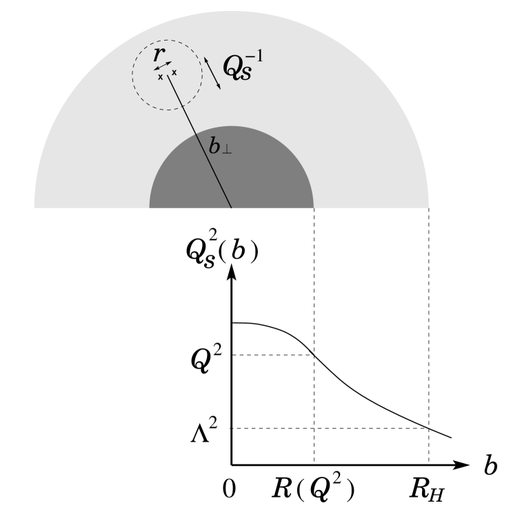
Figure 1: A pictorial representation of the dipole-hadron scattering in transverse projection (only half of the hadron disk is shown). The $b$–dependence of the saturation scale illustrated by the lower plot is the one to be found in Sect. 4.3.

The fact that $1/Q_{s}(\tau,b_{\perp})\ll 1/\Lambda_{QCD}$ implies that the transverse inhomogeneity in the hadron can be neglected when computing the contribution of such nearby sources to ${\rm d}{\cal N}_{\tau}(Q^{2},b_{\perp})$. That is, all the relevant sources act as being effectively at the same impact parameter, equal to $b_{\perp}$. This explains the factorized expression (2.14) for the scattering amplitude.

Since, moreover, ${\cal N}_{\tau}(Q^{2},z_{\perp})\ll 1$ for any $z_{\perp}$ satisfying (2.18), it follows that the function ${\cal N}_{\tau}(Q^{2})$ in eq. (2.14) can be computed by solving the linearized (and homogeneous) version of the BK equation, namely the BFKL equation without $b_{\perp}$ dependence.

Clearly, it was essential for the previous arguments that the dipole is “perturbative” : $Q^{2}\gg\Lambda_{QCD}^{2}$. This ensures that the separation $R_{H}(\tau)-R(\tau,Q^{2})$ between the black disk and the hadron edge (i.e., the width of the “grey area”) is sufficiently large for the condition $Q_{s}^{2}(\tau,b)\gg\Lambda_{QCD}^{2}$ to apply at all the points $b_{\perp}$ of interest. Besides, one can argue that $Q^{2}$ is the scale at which the QCD coupling should be evaluated (see the discussion in the Conclusions).

A factorization assumption similar to eq. (2.14) has been already used in the literature, in particular, in relation with the Froissart bound [11, 35], and also as an Ansatz in the search for approximate analytical [32] or numerical [36] solutions to the BK equation. But in previous work, this assumption was always based on experience with the (homogeneous) DGLAP equation, and not duly justified in the small-x regime.

That such a factorization is highly non-trivial in the presence of long-range gauge interactions is also emphasized by a recent controversy about this point, put forward in Ref. [14]. Specifically, in Ref. [14] it has been shown that, as far as the scattering of a coloured probe off the hadron is concerned, the long-range fields created by the saturated gluons provide a non-unitarizing contribution to the respective cross-section. On the basis of this example, the authors of Ref. [14] have concluded that the non-linear BK equation provides “saturation without unitarization”. In Sect. 3.2 below, we shall carefully and critically examine the arguments in Ref. [14], and demonstrate that, for the physically interesting case where the external probe is a (colourless) dipole, there is no problem with unitarity at all. The long-range interactions between the incoming dipole and the saturated gluons give only a small contribution to the scattering amplitude in the grey area, because the saturated gluons form themselves a dipole (i.e., they are globally colour neutral), and the dipole-dipole interaction falls off sufficiently fast with the separation between the two dipoles. The dominant contribution comes rather from the short-range scattering within the grey area (cf. eq. (2.18)), for which the factorization assumption (2.14) is indeed justified.

3 Quantum evolution and black disk radius

In the effective theory for the Colour Glass [18], the dipole-hadron scattering is described as scattering of the $q\bar{q}$ pair off a stochastic classical colour field which represents the small-x gluons in the hadron wavefunction. At high energy, one can use the eikonal approximation to obtain:

$${\cal N}_{\tau}(r_{\perp},b_{\perp})\,=\,1-{\cal S}_{\tau}(x_{\perp},y_{\perp}),\qquad{\cal S}_{\tau}(x_{\perp},y_{\perp})\equiv\frac{1}{N_{c}}\,\langle{\rm tr}\big{(}V^{\dagger}(x_{\perp})V(y_{\perp})\big{)}\rangle_{\tau},$$ (3.1)

with $r_{\perp}=x_{\perp}-y_{\perp}$ the size of the dipole and $b_{\perp}=(x_{\perp}+y_{\perp})/2$ the impact parameter (the quark is at $x_{\perp}$, and the antiquark at $y_{\perp}$). The $S$-matrix element ${\cal S}_{\tau}(x_{\perp},y_{\perp})$ involves the Wilson lines (path ordered exponentials along the straightline trajectories of the quark and the antiquark) $V^{\dagger}$ and $V$ built with the colour field of the target hadron. For instance,

$$V^{\dagger}(x_{\perp})\,=\,{\rm P}\exp\left\{ig\int_{0}^{\tau}d{\eta}\,\alpha^{a}_{{\eta}}(x_{\perp})t^{a}\right\},$$ (3.2)

where $\alpha_{{\eta}}(x_{\perp})$ is the stochastic “Coulomb field” created by color sources (mostly gluons) at rapidities $\tau^{\prime}<\tau$, and has longitudinal support at (space-time) rapidity $\eta\leq\tau$. Thus, the integral over $\eta$ in eq. (3.2) is in fact an integral over the longitudinal extent of the hadron (in units of space-time rapidity) seen by the external probe in a scattering at rapidity $\tau$. That is, the actual width of the hadron depends upon the energy of the collision. This is so since, with increasing energy, gluon modes with larger and larger longitudinal wavelengths participate in the collision, so that the hadron looks effectively thicker and thicker [10].

The brackets in the definition (3.1) of the $S$-matrix element refer to the average over all the configurations of the classical field with some appropriate probability distribution $W_{\tau}[\alpha]$ :

$$\langle{\rm tr}\big{(}V^{\dagger}(x_{\perp})V(y_{\perp})\big{)}\rangle_{\tau}\,=\,\int\,[{\rm d}\alpha]\,\,{\rm tr}\big{(}V^{\dagger}(x_{\perp})V(y_{\perp})\big{)}\,W_{\tau}[\alpha].$$ (3.3)

This probability distribution is not known directly, but its variation corresponding to integrating out gluons in the rapidity window $(\tau,\tau+d\tau)$ can be computed [34, 10]. This leads to a functional evolution equation for $W_{\tau}[\alpha]$ whose precise form is not needed here (see Ref. [10] for details). Suffices it to say that, via equations like (3.3), the functional equation for $W_{\tau}[\alpha]$ can be translated into an hierarchy of ordinary evolution equations for the $n$-point functions of the Wilson lines [10]. This procedure yields the same equations as obtained by Balitsky within a different approach, which focuses directly on the evolution of Wilson line operators [7]. (The fact that the infinite hierarchy of coupled equations by Balitsky can be reformulated as a single functional equation has been first recognized by Weigert [9].) In the limit where the number of colours $N_{c}$ is large, a closed equation can be written for the 2-point function (3.1) (with $\bar{\alpha}_{s}=N_{c}\alpha_{s}/\pi$) :

$${\partial\over{\partial\tau}}{\cal S}_{\tau}(x_{\perp},{y_{\perp}}) = -\bar{\alpha}_{s}\int{{d^{2}z_{\perp}}\over{2\pi}}{{(x_{\perp}-{y_{\perp}})^{2}}\over{(x_{\perp}-z_{\perp})^{2}({y_{\perp}}-z_{\perp})^{2}}}$$ (3.4)

$$\qquad\qquad\times\Big{(}{\cal S}_{\tau}(x_{\perp},{y_{\perp}})-{\cal S}_{\tau}(x_{\perp},z_{\perp}){\cal S}_{\tau}(z_{\perp},{y_{\perp}})\Big{)}.$$

The same equation has been derived independently by Kovchegov [8] within the Mueller’s dipole model [25]. We shall refer to eq. (3.4) as the Balitsky-Kovchegov (BK) equation.

3.1 Scattering in the grey area

In this subsection, we shall study the scattering amplitude in the grey area, and prove the factorization property (2.14). For more clarity, we shall formulate our arguments at the level of the BK equation. But one should keep in mind that our final conclusions are not specific to the large $N_{c}$ limit: the same results would have been obtained starting with the general non-linear evolution equations in Refs. [7, 9, 10].

Specifically, we shall use eq. (3.4) to demonstrate that the dominant contribution to $\partial{\cal S}_{\tau}/\partial\tau$ in the grey area comes from short-range scattering, i.e. from points $z_{\perp}$ such that

$$|z_{\perp}-b_{\perp}|\,\ll\,\frac{1}{Q_{s}(\tau,b_{\perp})}\,\ll\,\frac{1}{\Lambda_{QCD}}\,.$$ (3.5)

As explained in Sect. 2, the impact parameters of interest are such that the following inequalities are satisfied (with $Q^{2}\equiv 1/r_{\perp}^{2}$): $Q^{2}\gg Q_{s}^{2}(\tau,b)\gg\Lambda^{2}_{QCD}$. That is, the dipole is small not only as compared to the typical scale for non-perturbative physics and transverse inhomogeneity in the hadron, namely $1/{\Lambda_{QCD}}$, but also as compared to the shorter scale $1/Q_{s}(\tau,b_{\perp})$, which is the local saturation length. This implies that the dipole is only weakly interacting with the hadron: ${\cal S}_{\tau}(x_{\perp},{y_{\perp}})\simeq 1$, or ${\cal N}_{\tau}(r_{\perp},b_{\perp})\ll 1$. But this does not mean that we are a priori allowed to linearize eq. (3.4) with respect to ${\cal N}_{\tau}\,$. Indeed, the r.h.s. of this equation involves an integral over all $z_{\perp}$, so the virtual dipoles with transverse coordinates $({x_{\perp}},z_{\perp})$ or $(z_{\perp},{y_{\perp}})$ can be arbitrarily large. In fact, we shall see below that the dominant contribution comes nevertheless from $z_{\perp}$ which is relatively close to $b_{\perp}$, in the sense of eq. (3.5), but the upper limit $1/Q_{s}(\tau,b_{\perp})$ in this equation is a consequence of the non-linear effects.

To see this, it is convenient to divide the integral over $z_{\perp}$ in eq. (3.4) into two domains (“short-range” and “long-range”):

$${\rm(A)}\,\,\,\,|z_{\perp}-b_{\perp}|\,\ll\,1/Q_{s}(\tau,b_{\perp})\,,\qquad\ {\rm(B)}\,\,\,\,1/Q_{s}(\tau,b_{\perp})\,\ll\,|z_{\perp}-b_{\perp}|\,.$$ (3.6)

It is straightforward to compute the contribution of domain (B) to the r.h.s. of eq. (3.4): In this range, $|{x_{\perp}}-z_{\perp}|\sim|z_{\perp}-{y_{\perp}}|\sim|z_{\perp}-b_{\perp}|$, so the virtual dipoles are both relatively large, and therefore strongly absorbed. Thus, to estimate their contribution, one can set ${\cal S}_{\tau}(x_{\perp},z_{\perp})\approx 0$ and ${\cal S}_{\tau}(z_{\perp},{y_{\perp}})\approx 0$, and approximate the (“dipole” [24, 25, 19]) kernel in the BK equation as:

$${{(x_{\perp}-{y_{\perp}})^{2}}\over{(x_{\perp}-z_{\perp})^{2}({y_{\perp}}-z_{\perp})^{2}}}\,\approx\,{r_{\perp}^{2}\over(z_{\perp}-b_{\perp})^{4}}\,.$$ (3.7)

This gives (with $u_{\perp}^{2}\equiv(z_{\perp}-b_{\perp})^{2}>1/Q_{s}^{2}(\tau,b_{\perp})$) :

$$\left.\frac{\partial}{\partial\tau}{\cal S}_{\tau}(x_{\perp},{y_{\perp}})\right|_{\rm(B)} \simeq -\bar{\alpha}_{s}r_{\perp}^{2}{\cal S}_{\tau}(x_{\perp},{y_{\perp}})\int_{1/Q_{s}^{2}}\frac{du_{\perp}^{2}}{u_{\perp}^{4}}$$ (3.8)

$$= -\frac{\bar{\alpha}_{s}}{2}\,\Big{(}r_{\perp}^{2}Q_{s}^{2}(\tau,b_{\perp})\Big{)}{\cal S}_{\tau}(x_{\perp},{y_{\perp}}).$$

Since ${\cal S}_{\tau}(x_{\perp},{y_{\perp}})$ is of order one for the small dipole of interest, we deduce the following order-of-magnitude estimate (which we write for $\partial{\cal N}_{\tau}/\partial\tau$, for further convenience) :

$$\left.\frac{\partial}{\partial\tau}{\cal N}_{\tau}(r_{\perp},b_{\perp})\right|_{\rm(B)} \sim \bar{\alpha}_{s}\,r_{\perp}^{2}Q_{s}^{2}(\tau,b_{\perp}).$$ (3.9)

Note that, even for this “long range” contribution, the integral in eq. (3.8) is dominated by points $u_{\perp}$ which are relatively close to the lower limit $1/Q_{s}(\tau,b_{\perp})\,$; this is so because the dipole kernel (3.7) is rapidly decreasing at large distances $|z_{\perp}-b_{\perp}|\gg r_{\perp}$.

To evaluate the corresponding contribution of domain (A), we note first that, in this domain, all the dipoles are small, so the scattering amplitude is small, ${\cal N}_{\tau}\ll 1$, for any of them. It is therefore appropriate to linearize the r.h.s. of eq. (3.4) with respect to ${\cal N}_{\tau}$ (below, $u_{\perp}={x_{\perp}}-z_{\perp}$):

$$\left.\frac{\partial}{\partial\tau}{\cal N}_{\tau}(r_{\perp},b_{\perp})\right|_{\rm(A)} \!\!\simeq\!\! -\bar{\alpha}_{s}\int^{1/Q_{s}}\frac{d^{2}u_{\perp}}{2\pi}\,\frac{r_{\perp}^{2}}{u_{\perp}^{2}(r_{\perp}-u_{\perp})^{2}}\,$$

$$\!\!\!\!\times\left\{{\cal N}_{\tau}(r_{\perp},b_{\perp})-{\cal N}_{\tau}\Big{(}u_{\perp},b_{\perp}-\frac{u_{\perp}-r_{\perp}}{2}\Big{)}-{\cal N}_{\tau}\Big{(}r_{\perp}-u_{\perp},b_{\perp}-\frac{u_{\perp}}{2}\Big{)}\right\}.$$

This is recognized as the BFKL equation in the coordinate representation. Since both $u_{\perp}$ and $r_{\perp}$ are small as compared to $1/Q_{s}(\tau,b_{\perp})$, and therefore much smaller than $1/{\Lambda_{QCD}}$, it is appropriate to neglect the hadron inhomogeneity when evaluating the r.h.s. of this equation. That is, all the functions ${\cal N}_{\tau}$ in the r.h.s can be evaluated at the same impact parameter, namely $b_{\perp}$.

To obtain an order-of-magnitude estimate for the r.h.s. of eq. (3.1), we need an estimate for the function ${\cal N}_{\tau}(r_{\perp},b_{\perp})$ in the regime where $r_{\perp}\ll 1/Q_{s}(\tau,b_{\perp})$. An approximate solution valid in this regime will be constructed in Sect. 4. But for the present purposes, we do not need all the details of this solution. Rather, it is enough to use the following “scaling approximation”

$${\cal N}_{\tau}(r_{\perp},b_{\perp}) \simeq \left(r_{\perp}^{2}Q_{s}^{2}(\tau,b_{\perp})\right)^{\lambda},$$ (3.11)

with $\lambda\leq 1$. In Ref. [29], this approximation has been justified for a homogeneous hadron (no dependence upon $b_{\perp}$). In Sect. 5 below, we shall find that, in the regime of interest, geometric scaling remains true also in the presence of inhomogeneity.

The highest value $\lambda=1$ corresponds to the “double logarithmic regime” in which the dipole is extremely small, $\ln(Q^{2}/Q_{s}^{2}(\tau,b_{\perp}))\gg 1$, or, equivalently, its impact parameter $b_{\perp}$ is far outside the black disk, $b\gg R(\tau,Q^{2})$. Here, however, we are mostly interested in points $b_{\perp}$ which are not so far away from the black disk, since we would like to study how the latter expands by incorporating points from the grey area. In this regime, i.e., for $b>R(\tau,Q^{2})$ but such that $(b-R(\tau,Q^{2}))/R(\tau,Q^{2})\ll 1$, the scattering amplitude is given by eq. (3.11) with a power $\lambda$ which is strictly smaller than one (see Sect. 5).

To simplify the evaluation of eq. (3.1), we shall divide domain (A) in two subdomains, in which further approximations are possible: (A.I) one of the two virtual dipoles, say $u_{\perp}$, is much smaller than the other one : $u_{\perp}\ll r_{\perp}$; (A.II) both virtual dipoles are larger than the original one, although still smaller than one saturation length: $r_{\perp}\ll u_{\perp}\sim|u_{\perp}-r_{\perp}|\ll 1/Q_{s}(\tau,b_{\perp})$.

In domain (A.I), the first and third “dipoles” in the r.h.s. of eq. (3.1) cancel each other (since $r_{\perp}^{2}\approx(r_{\perp}-u_{\perp})^{2}$), and we are left with

$$\left.\frac{\partial}{\partial\tau}{\cal N}_{\tau}(r_{\perp},b_{\perp})\right|_{\rm(A.I)}\,\simeq\,2\bar{\alpha}_{s}\int^{r_{\perp}}\frac{d^{2}u_{\perp}}{2\pi}\,\frac{1}{u_{\perp}^{2}}\,\left(u_{\perp}^{2}Q_{s}^{2}(\tau,b_{\perp})\right)^{\lambda}\,\sim\,\bar{\alpha}_{s}\left(r_{\perp}^{2}Q_{s}^{2}(\tau,b_{\perp})\right)^{\lambda},$$ (3.12)

where the factor of 2 takes into account that one can choose any of the two virtual dipoles as the small one.

In domain (A.II), one can neglect ${\cal N}_{\tau}(r_{\perp},b_{\perp})\ll{\cal N}_{\tau}(u_{\perp},b_{\perp})\simeq{\cal N}_{\tau}(u_{\perp}-r_{\perp},b_{\perp})$, and obtain:

$$\left.\frac{\partial}{\partial\tau}{\cal N}_{\tau}(r_{\perp},b_{\perp})\right|_{\rm(A.II)} \simeq 2\bar{\alpha}_{s}\int^{1/Q_{s}}_{r_{\perp}}\frac{d^{2}u_{\perp}}{2\pi}\,\frac{r_{\perp}^{2}}{u_{\perp}^{4}}\,\left(u_{\perp}^{2}Q_{s}^{2}(\tau,b_{\perp})\right)^{\lambda}$$ (3.13)

$$= \bar{\alpha}_{s}\left(r_{\perp}^{2}Q_{s}^{2}(\tau,b_{\perp})\right)^{\lambda}\,\frac{1-(r_{\perp}^{2}Q_{s}^{2}(\tau,b_{\perp}))^{1-\lambda}}{1-\lambda}\,,$$

which is of the same order as the (A.I)–contribution (3.12) when $\lambda<1$, but is logarithmically enhanced over it, and also over the long-range contribution (3.9), when $\lambda\to 1$ :

$$\left.\frac{\partial}{\partial\tau}{\cal N}_{\tau}(r_{\perp},b_{\perp})\right|_{\rm(A.II)}\,\sim\,\bar{\alpha}_{s}\left(r_{\perp}^{2}Q_{s}^{2}(\tau,b_{\perp})\right)\ln\frac{1}{r_{\perp}^{2}Q_{s}^{2}(\tau,b_{\perp})}\,\qquad{\rm when}\quad\lambda=1.$$ (3.14)

By comparing eqs. (3.9) and (3.12)–(3.14), it should be clear by now that, for any $\lambda\leq 1$, the short-range contribution, domain (A), dominates over the long-range one, domain (B). In other words, from the analysis of the non-linear BK equation, we have found that, for a “small” incoming dipole, the dominant contribution to the quantum evolution of ${\cal N}_{\tau}(r_{\perp},b_{\perp})$ comes from still “small” virtual dipoles $\{(x_{\perp},z_{\perp}),(z_{\perp},{y_{\perp}})\}$ (see Figure 1). This has two important consequences. (i) One can linearize the BK equation with respect to ${\cal N}_{\tau}$, as we did already in eq. (3.1). This gives the BFKL equation. (ii) One can ignore the transverse inhomogeneity in the BFKL equation. That is, one can replace eq. (3.1) by

$$\frac{\partial}{\partial\tau}{\cal N}_{\tau}(r_{\perp},b_{\perp}) \simeq \bar{\alpha}_{s}\int\frac{d^{2}z_{\perp}}{2\pi}\frac{r_{\perp}^{2}}{(z_{\perp}-x_{\perp})^{2}(z_{\perp}-{y_{\perp}})^{2}}$$ (3.15)

$$\quad\times\Big{\{}{\cal N}_{\tau}(z_{\perp}-x_{\perp},b_{\perp})+{\cal N}_{\tau}(z_{\perp}-{y_{\perp}},b_{\perp})-{\cal N}_{\tau}(r_{\perp},b_{\perp})\Big{\}},$$

in which all the amplitudes ${\cal N}_{\tau}$ are evaluated at the same impact parameter, namely at $b_{\perp}$.

Note that, as compared to eq. (3.13), there is no need to insert an upper cutoff $\sim 1/Q_{s}$ in the integral in eq. (3.15). This is so since, to the accuracy of interest, the solution ${\cal N}_{\tau}(r_{\perp},b_{\perp})$ to eq. (3.15) is actually insensitive to such a cutoff. One can understand this on the basis of eq. (3.13) : For large $r_{\perp}$ (with $r_{\perp}^{2}Q_{s}^{2}(\tau,b_{\perp})\ll 1$ though), the solution has the “scaling” behaviour in eq. (3.11) with a power $\lambda$ which is strictly smaller than one (see the discussion in Sects. 4 and 5). Then the integral in eq. (3.13) is dominated by points $u_{\perp}$ which are close to the lower limit $r_{\perp}$, i.e., by virtual dipoles which are not much larger than the incoming dipole. The dependence upon the upper cutoff $\sim 1/Q_{s}$ is therefore a subleading effect, which can be safely ignored.

We finally come to the last step in our argument: Since the dependence of eq. (3.15) upon $b_{\perp}$ is only “parametric”, it is clear that the impact parameter dependence of the solution is entirely fixed by the initial condition. This, together with eq. (2.8), implies that ${\cal N}_{\tau}(r_{\perp},b_{\perp})$ has the factorized structure:

$${\cal N}_{\tau}(r_{\perp},b_{\perp})=S(b_{\perp}){\cal N}_{\tau}(r_{\perp})$$ (3.16)

where $S(b_{\perp})$ is the transverse profile of the initial condition, while ${\cal N}_{\tau}(r_{\perp})$ satisfies the homogeneous BFKL equation and will be discussed in Sect. 4. A brief inspection of the previous arguments reveals that the terms neglected in our approximations are suppressed by either powers of $r_{\perp}^{2}Q_{s}^{2}(\tau,b_{\perp})$ (e.g., the long-range contribution (3.9), or the cutoff–dependent term in eq. (3.13)), or by powers of ${\Lambda^{2}_{QCD}}/Q_{s}^{2}(\tau,b_{\perp})$ (the inhomogeneous effects in eq. (3.1)). This specifies the accuracy of the factorized approximation in eq. (3.16).

3.2 More on the saturated gluons

In the previous subsection, we have seen that colour sources located far away from the impact parameter of the dipole, such as $|z_{\perp}-b_{\perp}|>1/Q_{s}(\tau,b_{\perp})$, do not significantly contribute to the scattering amplitude in the grey area. In what follows, we shall examine more carefully a particular contribution of this type, namely, that associated with the saturated gluons within the black disk: $|z_{\perp}|<R(\tau,Q^{2})$. Indeed, it has been recently argued [14] that, by itself, this contribution would lead to unitarity violations. To clarify this point, we shall compute this contribution within the effective theory for the Colour Glass Condensate, where the physical interpretation of the result is transparent. The same result will be then reobtained from the BK equation. Our analysis will confirm that, for impact parameters $b_{\perp}$ within the grey area, this long-range contribution is indeed subleading, and can be safely neglected at high energies. As we shall see, non-unitary contributions of the type discussed in Ref. [14] appear only in the physically uninteresting case where the exernal probe carries a non-zero colour charge (as opposed to the colourless dipole).

According to eqs. (3.1) and (3.2), the scattering amplitude at rapidity $\tau$ depends upon the Coulomb field $\alpha_{\eta}^{a}(x_{\perp})$ at all the space-time rapidities $\eta\leq\tau$. In general, this is related to the colour sources in the hadron via the two-dimensional Poisson equation $-\nabla^{2}_{\perp}\alpha_{\eta}^{a}(x_{\perp})=\rho_{\eta}^{a}(x_{\perp})$, with the solution:

$$\alpha_{\eta}^{a}(x_{\perp}) = \int d^{2}z_{\perp}\langle x_{\perp}|\frac{1}{-\nabla^{2}_{\perp}}|z_{\perp}\rangle\,\rho_{\eta}^{a}(z_{\perp}).$$ (3.17)

In this equation, $\rho_{\eta}^{a}(x_{\perp})$ is the colour charge density (per unit transverse area per unit space-time rapidity) of the colour sources at space-time rapidity $\eta$. Here, we are only interested in such colour sources which are saturated. To isolate their contribution, it is important to remark that these sources have been generated by the quantum evolution up to a “time” equal to $\eta$, so the corresponding saturation scale is $Q_{s}(\eta,b_{\perp})$ (and not $Q_{s}(\tau,b_{\perp})$). Thus, the integration in eq. (3.17) must be restricted to $|z_{\perp}|\leq R(\eta,Q^{2})$, with $R(\eta,Q^{2})$ the black disk radius at rapidity $\eta$ (cf. eq. (2.10)), and $Q^{2}$ the typical momentum carried by the Fourier modes of $\alpha_{\eta}^{a}(x_{\perp})$ (as usual, this is fixed by the transverse size of the incoming dipole).

There is a similar restriction on the values of $\eta$ : For given $Q^{2}$, there is a minimum rapidity $\bar{\tau}_{1}(Q^{2})$ below which there is no black disk at all: $R(\eta,Q^{2})=0$ for $\eta<\bar{\tau}_{1}(Q^{2})$. This is the rapidity at which the black disk first emerges at the center of the hadron, namely, at which $Q_{s}^{2}(\bar{\tau}_{1},b=0)=Q^{2}$ (see Sect. 4.4 below). Thus, in order to count saturated sources only, the integral over $\eta$ in Wilson lines like (3.2) must be restricted to the interval $\bar{\tau}_{1}(Q^{2})<\eta<\tau$. In Fig. 2, the saturated sources (with momentum $Q^{2}$) occupy the lower right corner, below the dashed line which represents the profile of the black disk as a function of $\eta$.

Figure 2: The longitudinal profile of the hadron as it appears in a scattering at given $\tau$ and $Q^{2}$. The longitudinal coordinate is on the horizontal axis, and is measured in units of space-time rapidity. The tranverse coordinate is on the vertical axis. A longitudinal layer at rapidity $\eta$ is delimited for more clarity. The wavy line represents the colour field $\alpha_{\eta}$ created at point ${x_{\perp}}$ by the (saturated) source $\rho_{\eta}$ at $z_{\perp}$. The enclined dashed line represents the limit of the black disk, which increases linearly with $\eta$, as we shall see in Sect. 4.

The external point $x_{\perp}$ in eq. (3.17) is at the impact parameter of the quark (or the antiquark) in the dipole, so it satisfies $|x_{\perp}|\gg R(\tau,Q^{2})\geq R(\eta,Q^{2})$ for any $\eta\leq\tau$. It is therefore appropriate to evaluate the field (3.17) in a multipolar expansion:

$$\alpha_{\eta}^{a}(x_{\perp}) \!=\! \langle x_{\perp}|\frac{1}{-\nabla^{2}_{\perp}}|0_{\perp}\rangle\int^{R}\!{d^{2}z_{\perp}}\,\rho_{\eta}^{a}(z_{\perp})-{\partial\over\partial x^{i}}\langle x_{\perp}|\frac{1}{-\nabla^{2}_{\perp}}|0_{\perp}\rangle\int^{R}\!{d^{2}z_{\perp}}z^{i}\rho_{\eta}^{a}(z_{\perp})\,+\cdots$$ (3.18)

$$\!\equiv\! \langle x_{\perp}|\frac{1}{-\nabla^{2}_{\perp}}|0_{\perp}\rangle\ {\cal Q}^{a}+{x^{i}\over 2\pi x_{\perp}^{2}}\,{\cal D}^{i}_{a}\,+\cdots,$$

where $R\equiv R(\eta,Q^{2})$, ${\cal Q}^{a}$ is the total colour charge within the black disk, ${\cal D}^{i}_{a}$ is the corresponding dipolar moment, etc.

To compute the scattering amplitude (3.1), one has to construct the Wilson lines $V^{\dagger}$ and $V$ with the field (3.18) and then average over $\alpha$ (or, equivalently, over $\rho$) as in eq. (3.3). In what follows, it is more convenient to work with the probability distribution for $\rho$, i.e., $W_{\tau}[\rho]$. In general, this distribution is determined by a complicated functional evolution equation, which is very non-linear [9, 10].

However, as observed in Ref. [22], this equation simplifies drastically in the saturation regime, where the corresponding solution $W_{\tau}[\rho]$ is essentially a Gaussian in $\rho$. This can be understood as follows: The non-linear effects in the quantum evolution enter via Wilson lines like eq. (3.2). At saturation, the field $\alpha$ in the exponential carries typical momenta $k_{\perp}\sim Q_{s}$ and has a large amplitude $\alpha\sim 1/g$. Thus, the Wilson lines are strongly varying over a transverse distance $1/Q_{s}(\tau,b_{\perp})$. When observed by a probe with transverse resolution $Q^{2}\ll Q_{s}^{2}(\tau,b_{\perp})$, these Wilson lines are rapidly oscillating and average to zero. Thus, at saturation, one can drop out the Wilson lines, and all the associated non-local and non-linear effects. Then, the probability distribution $W_{\tau}[\rho]$ becomes indeed a Gaussian, which by the same argument is local in colour and space-time rapidity, and also homogeneous in all the (longitudinal and transverse) coordinates. The only remaining correlations are those in the transverse plane, and, importantly, these are such as to ensure colour neutrality [18].

Specifically, the only non-trivial correlation function of the saturated sources is the two-point function, which reads [22] (see also Sect. 5.4 in Ref. [18]) :

$$\langle\rho_{\eta}^{a}(z_{\perp})\,\rho_{{\eta}^{\prime}}^{b}(u_{\perp})\rangle_{\tau} = \delta^{ab}\delta({\eta}-{\eta}^{\prime})\,\lambda(z_{\perp}-u_{\perp}),$$

$$\lambda(k_{\perp}) = \frac{1}{\pi}\,k_{\perp}^{2}.$$ (3.19)

For given $\eta$ and $k_{\perp}^{2}\sim Q^{2}$, eq. (3.2) holds for points $z_{\perp}$ and $u_{\perp}$ within the black disk of radius $R(\eta,Q^{2})$. The crucial property of the 2-point function (3.2) is that it vanishes as $k_{\perp}^{2}\to 0$. Physically, this means that, globally, the saturated gluons are colour neutral, as anticipated: $\langle{\cal Q}^{a}{\cal Q}^{a}\rangle=0$, where ${\cal Q}^{a}$ is the total colour charge (at given $\eta$) in the transverse plane. In fact, since the Wilson lines average to zero over distances $\Delta b_{\perp}\mathrel{\hbox to0.0pt{\raise 2.20013pt\hbox{$>$}\hss}{\lower 2.20013pt\hbox{$\sim$}}}1/Q_{s}(\eta,b_{\perp})$, it follows that colour neutrality is achieved already over a transverse scale of the order of the saturation length:

$$\int_{\Delta S_{\perp}}\!{d^{2}x_{\perp}}\int_{\Delta S_{\perp}}\!{d^{2}y_{\perp}}\,\langle\rho_{\eta}^{a}(x_{\perp})\rho_{\eta}^{a}(y_{\perp})\rangle\,=\,0,$$ (3.20)

where $\Delta S_{\perp}$ is, e.g., a disk of radius $R>1/Q_{s}(\eta,b_{\perp})$ centered at $b_{\perp}$.

This immediately implies that, as soon as the black disk is large enough, the overall charge of the saturated gluons vanishes, ${\cal Q}^{a}=0$, so we can ignore the monopole field in eq. (3.18). Here, “large enough” means, e.g., $R(\tau,Q^{2})\gg 1/Q$, which guarantees that the radius of the black disk is larger than the saturation length $1/Q_{s}(\eta,b_{\perp})$ at any $b_{\perp}$ within the disk and at any $\eta$ in the interval $\bar{\tau}_{1}(Q^{2})<\eta<\tau$ (since then $Q_{s}(\eta,b_{\perp})>Q$). In these conditions, the dominant field of the saturated gluons at large distances is the dipolar field in eq. (3.18).

Below, we shall need the two-point function of this field:

$$\langle\alpha_{\eta}^{a}(x_{\perp})\,\alpha_{\eta^{\prime}}^{b}(y_{\perp})\rangle_{\tau} \equiv \delta^{ab}\delta(\eta-\eta^{\prime})\,\gamma_{\eta}(x_{\perp}-y_{\perp}).$$ (3.21)

From eq. (3.18), we deduce (with colour indices omitted, since trivial):

$$\gamma_{\eta}(x_{\perp}-y_{\perp})\,=\,{x^{i}\over 2\pi x_{\perp}^{2}}{y^{j}\over 2\pi y_{\perp}^{2}}\,\langle{\cal D}^{i}{\cal D}^{j}\rangle,$$ (3.22)

with (cf. eq. (3.2)):

$$\langle{\cal D}^{i}{\cal D}^{j}\rangle \equiv \int^{R}{d^{2}z_{\perp}}\int^{R}{d^{2}u_{\perp}}\ z^{i}u^{j}\ \lambda(z_{\perp}-u_{\perp})$$ (3.23)

$$= \int^{R}{d^{2}z_{\perp}}\int^{R}{d^{2}u_{\perp}}\ \int^{Q_{s}}{d^{2}k_{\perp}\over(2\pi)^{2}}\ {\rm e}^{ik_{\perp}\cdot(z_{\perp}-u_{\perp})}{\partial^{2}\over\partial k^{i}\partial k^{j}}\,\frac{k_{\perp}^{2}}{\pi}$$

$$\simeq \delta^{ij}\,2R^{2}(\eta,Q^{2})\,.$$

where $R\equiv R(\eta,Q^{2})$, $Q_{s}\equiv Q_{s}(\eta,b_{\perp})$ (with $b_{\perp}\equiv(z_{\perp}+u_{\perp})/2<R$), and formal manipulations like integrations by parts or the use of the Fourier representation of the $\delta$-function were permitted since $RQ_{s}\gg 1$. Thus, finally,

$$\gamma_{\eta}(x_{\perp},y_{\perp})={1\over 2\pi^{2}}\ \frac{{x_{\perp}}\cdot{y_{\perp}}}{x_{\perp}^{2}y_{\perp}^{2}}\ R^{2}({\eta},Q^{2}),$$ (3.24)

which, we recall, is valid only as long as $x_{\perp},\,y_{\perp}\gg R({\eta},Q^{2})$.

We are now in a position to compute the scattering amplitude (3.1) for the scattering between the incoming dipole and the dipolar colour charge distribution within the black disk. To this aim, we have to average the product ${\rm tr}\big{(}V^{\dagger}(x_{\perp})V(y_{\perp})\big{)}$ over the Gaussian random variable $\alpha_{\eta}$ with two-point function (3.21). The result of this calculation is well-known (see, e.g., [18]):

$$\tilde{\cal S}_{\tau}(x_{\perp},y_{\perp})={\rm exp}\left\{-{g^{2}C_{F}\over 2}\int_{\bar{\tau}}^{\tau}d{\eta}\Big{[}\gamma_{\eta}(x_{\perp},x_{\perp})+\gamma_{\eta}(y_{\perp},y_{\perp})-2\gamma_{\eta}(x_{\perp},y_{\perp})\Big{]}\right\}$$ (3.25)

where $C_{F}\equiv t^{a}t^{a}=(N_{c}^{2}-1)/2N_{c}$ and the lower limit $\bar{\tau}$ in the integral is a shorthand for $\bar{\tau}_{1}(Q^{2})$ with $Q^{2}=1/r_{\perp}^{2}$. The “tilde” symbol on ${\cal S}$ is to remind that this is not the total $S$-matrix element, but just the particular contribution to it coming from the saturated gluons. An immediate calculation using eqs. (3.24) and (3.25) yields (with $\bar{\alpha}_{s}\equiv 2\alpha_{s}C_{F}/\pi\simeq\alpha_{s}N_{c}/\pi$ in the large $N_{c}$ limit) :

$$\tilde{\cal S}_{\tau}(x_{\perp},y_{\perp}) = {\rm exp}\left\{-\bar{\alpha}_{s}\ \frac{(x_{\perp}-y_{\perp})^{2}}{2x_{\perp}^{2}y_{\perp}^{2}}\ \int_{\bar{\tau}}^{\tau}d{\eta}\ R^{2}({\eta},Q^{2})\right\}$$ (3.26)

$$\simeq {\rm exp}\left\{-\bar{\alpha}_{s}\ \frac{r_{\perp}^{2}}{2b_{\perp}^{4}}\ \int_{\bar{\tau}}^{\tau}d{\eta}\ R^{2}({\eta},Q^{2})\right\},$$

where in the second line we have replaced in the denominator $x_{\perp}^{2}\simeq y_{\perp}^{2}\simeq b_{\perp}^{2}$ (which is appropriate since $b_{\perp}\gg R({\tau},Q^{2})\gg r_{\perp}$). The exponent in eq. (3.26) vanishes when the dipole shrinks to a point, $r_{\perp}\to 0$. This is the expected dipole cancellation, manifest already on eq. (3.25).

The previous derivation makes the physical interpretation of eq. (3.26) very clear: The exponent there is the square of the potential $\sim gt^{a}r_{\perp}\frac{1}{b^{2}}R(\eta)$ for the interaction between two dipoles — the “external dipole” of size $r_{\perp}$ and the dipole made of the saturated gluons (at a given space-time rapidity $\eta$), with size $R(\eta)$ — separated by a large distance $b$. There exists one layer of saturated gluons at any $\eta$ within the interval $\bar{\tau}_{1}(Q^{2})<\eta<\tau$, so eq. (3.26) involves an integral over this interval.

Of course, eq. (3.26) can be also obtained directly from the BK equation, although, in that context, its physical interpretation in terms of dipole–dipole scattering may not be so obvious. In fact, this is just a particular piece of what we have called “the contribution (B)” in the previous subsection, i.e., the contribution of the points $z_{\perp}$ satisfying $|z_{\perp}-b_{\perp}|\gg 1/Q_{s}(\tau,b_{\perp})$. If $z_{\perp}$ now refers to the saturated gluons within the black disk, then it is further restricted by $|z_{\perp}|<R(\tau,Q^{2})$, which implies $|z_{\perp}-b_{\perp}|\approx b$ for the same reasons as above. Then, a simple calculation similar to eq. (3.8) immediately yields

$$\frac{\partial}{\partial\tau}\tilde{\cal S}_{\tau}(x_{\perp},y_{\perp}) \simeq -\bar{\alpha}_{s}\,\frac{r_{\perp}^{2}}{b_{\perp}^{4}}\,R^{2}(\tau,Q^{2})\,\tilde{\cal S}_{\tau}(x_{\perp},y_{\perp}),$$ (3.27)

which after integration over $\tau$ is indeed equivalent to eq. (3.26) .

For comparison with eq. (3.26), it is interesting to compute also the $S$-matrix element for a coloured external probe, e.g., a quark, which scatters off the saturated gluons in the eikonal approximation. A calculation entirely similar to that leading to eq. (3.26) yields ($b_{\perp}$ is the transverse location of the quark):

$$\frac{1}{N_{c}}\,\Big{\langle}{\rm tr}\,V^{\dagger}(b_{\perp})\Big{\rangle}_{\tau} = {\rm exp}\left\{-{g^{2}C_{F}\over 2}\int_{\bar{\tau}}^{\tau}d{\eta}\ \gamma_{\eta}(b_{\perp},b_{\perp})\right\}$$ (3.28)

$$\simeq {\rm exp}\left\{-\bar{\alpha}_{s}\ \frac{1}{2b_{\perp}^{2}}\ \int_{\bar{\tau}}^{\tau}d{\eta}\ R^{2}({\eta},Q^{2})\right\}$$

where the second line follows after using eq. (3.24).

To summarize, the amplitude for the scattering off the saturated gluons decreases like $1/b_{\perp}^{4}$ for an external dipole, but only as $1/b_{\perp}^{2}$ for a coloured probe. This difference turns out to be essential: because of it, this long-range scattering plays only a marginal role for the dipole, while it leads to unitarity violations in the case of the coloured probe (although the very question of unitarization makes little physical sense for a “probe” which is not a colour singlet).

To see this, assume the long-range contributions shown above to be the only contributions, or, in any case, those which give the dominant contribution to the cross-section. Then, one can rely on the previous formulae to estimate the rate of expansion of the black disk. Namely, assume that, for the purpose of getting an order-of-magnitude estimate, one can extrapolate eqs. (3.26) and (3.28) up to energies where the black disk approaches the incidence point $b_{\perp}$ of the external probe. Then, we expect the exponents in these equations to become of order one for $b\sim R({\tau},Q^{2})$. For the external dipole, this condition implies:

$$\bar{\alpha}_{s}\ \frac{r_{\perp}^{2}}{R^{4}(\tau,Q^{2})}\int_{\bar{\tau}}^{\tau}d{\eta}\ R^{2}({\eta},Q^{2})\,\sim\,1.$$ (3.29)

This gives (recall that $Q^{2}={1/r_{\perp}^{2}}$):

$$Q^{4}R^{4}(\tau,Q^{2})\,=\,\bar{\alpha}_{s}\int_{\bar{\tau}}^{\tau}d{\eta}\ Q^{2}R^{2}({\eta},Q^{2}),$$ (3.30)

or, after taking a derivative w.r.t. $\tau\,$,

$$2\,\frac{d}{d\tau}\,\Big{(}Q^{2}R^{2}(\tau,Q^{2})\Big{)}\,=\,\bar{\alpha}_{s},$$ (3.31)

whose solution $R^{2}(\tau,Q^{2})$ increases linearly with $\tau$.

By contrast, for a coloured probe, the same condition yields:

$$\bar{\alpha}_{s}\int_{\bar{\tau}}^{\tau}d{\eta}\ R^{2}({\eta},Q^{2})\,=\,{R^{2}(\tau,Q^{2})}\,$$ (3.32)

or after taking a derivative w.r.t. $\tau$:

$$\frac{d}{d\tau}\,R^{2}(\tau,Q^{2})\,=\,\bar{\alpha}_{s}\,R^{2}(\tau,Q^{2}),$$ (3.33)

which gives an exponential increase with $\tau$, as found in Ref. [14].

We thus see that the violation of unitarity by long-range Coulomb scattering reported by the authors of Ref. [14] is related to their use of an external probe which carries a non-zero colour charge. This case is physically ill defined, and therefore uninteresting (note, indeed, that $\langle{\rm tr}\,V^{\dagger}\rangle$ is not a gauge-invariant quantity); in particular, its relevance for the problem of gluon saturation in the target wavefunction remains unclear to us (since the relation between “blackness” and saturation holds only for dipole probes; cf. the discussion prior to eq. (2.9)).

On the other hand, for the physically interesting case of an external dipole, the contribution (3.31) to the expansion of the black disk not only is consistent with unitarity — if this was the only contribution, the cross-section $\propto R^{2}(\tau,Q^{2})$ would increase linearly with $\tau$ —, but at large $\tau$, is even negligible as compared to the corresponding contribution of the short-range scattering (which gives a cross-section increasing like $\tau^{2}$, cf. eqs. (2.16)–(2.17)).

These considerations are conveniently summarized in the following, schematic, approximation to the scattering amplitude in the grey area, which follows from the previous analysis in this section: ${\cal N}_{\tau}(r_{\perp},b_{\perp})$ is the sum of two contributions, a short-range contribution, cf. eq. (2.15), and a long-range one, cf. eq. (3.26) :

$${\cal N}_{\tau}(r_{\perp},b_{\perp})\,\approx\,\sqrt{r_{\perp}^{2}\Lambda^{2}}\,{\rm e}^{\omega\bar{\alpha}_{s}\tau}\,{\rm e}^{-2m_{\pi}b}\,+\,\bar{\alpha}_{s}\,\frac{r_{\perp}^{2}}{2b_{\perp}^{4}}\int_{\tau_{0}}^{\tau}d{\eta}\ R^{2}({\eta},Q^{2})\,,$$ (3.34)

with the short-range contribution determined by the solution to the homogeneous BFKL equation (3.15) together with the assumed exponential fall-off of the initial condition (see Sects. 4 and 5 below for more details), and the long-range contribution obtained by keeping only the lowest-order term in eq. (3.26) (which is enough since we are in a regime where ${\cal S}_{\tau}(x_{\perp},y_{\perp})\sim 1$). At the initial rapidity $\tau_{0}$, the long-range contribution vanishes, while the short-range contribution reduces to ${\rm e}^{-2m_{\pi}(b-R(\tau_{0},Q^{2}))}$ with $R(\tau_{0},Q^{2})$ given by eq. (2.16), as it should.

For given $\tau$ and $r_{\perp}=1/Q$, eq. (3.34) applies at impact parameters in the grey area, $R(\tau,Q^{2})<b<R_{H}(\tau)$, but it can be extrapolated to estimate the boundaries of this area, according to eqs. (2.9)–(2.12). It is easy to check that, at high energy, both these boundaries are determined by the short-range contribution, i.e., the first term in the r.h.s. of eq. (3.34). Thus, this contribution dominates the scattering amplitude at any $b_{\perp}$ in the grey area. By comparison, the long-range contribution is suppressed by one power of $1/\bar{\alpha}_{s}\tau$.

For instance, the black disk radius is obtained by requiring ${\cal N}_{\tau}(r_{\perp},b_{\perp})\sim 1$ for $b_{\perp}\sim R(\tau,Q^{2})$ (cf. eq. (2.9)). If one assumes the short-range contribution to dominate in this regime, one obtains the estimate (2.16) for the black disk radius: $R(\tau,Q^{2})\simeq(\omega/2m_{\pi})\bar{\alpha}_{s}\tau$. By using this result, one can evaluate the corresponding long-range contribution, and thus check that this is comparatively small, as it should for consistency with the original assumption:

$$\bar{\alpha}_{s}\ \frac{r_{\perp}^{2}}{R^{4}(\tau,Q^{2})}\int^{\tau}d{\eta}\ R^{2}({\eta},Q^{2})\,\bigg{|}_{R(\tau,Q^{2})\sim\,\,\bar{\alpha}_{s}\tau/m_{\pi}}\,\,\sim\,\,\frac{r_{\perp}^{2}m_{\pi}^{2}}{\bar{\alpha}_{s}\tau}\,\,\ll\,\,1.$$ (3.35)

By contrast, if one starts by assuming that the long-range contribution dominates, then one is running into a contradiction, since in this case $R(\tau,Q^{2})\propto\sqrt{\bar{\alpha}_{s}\tau}$, cf. eq. (3.31), and the short-range contribution increases exponentially along the “trajectory” $b=R(\tau,Q^{2})$.

A similar conclusion holds for $b=R_{H}(\tau)$ [since $R_{H}(\tau)=R(\tau,Q^{2}=\Lambda^{2}_{QCD})$, cf. eq. (2.12)], and therefore for any point $b_{\perp}$ within the grey area. (The hadron radius $R_{H}(\tau)$ will be evaluated in Sect. 4.2 below.) Thus, the short-range contribution is indeed the dominant one in the grey area. This contribution preserves the exponential fall-off of the initial condition, and therefore saturates the Froissart bound, as explained in Sect. 2.

It is essential for the consistency of the previous arguments — which combine perturbative quantum evolution with non-perturbative initial conditions — that perturbation theory has been applied only in the regime where it is expected to be valid, namely, in the central region at $b<R_{H}(\tau)$, where the gluon density is high and the local saturation scale $Q_{s}(\tau,b)$ is much larger than $\Lambda_{QCD}$. It has been enough to consider this region for the present purposes since this includes both the black disk and the grey area which controls its expansion. Within this region, the perturbative evolution equations of Refs. [7, 8, 9, 10] can be trusted, and the additional approximations that we have performed on these equations are under control as well. When supplemented with appropriate boundary conditions — which are truly non-perturbative, since reflecting the physics of confinement —, these equations allow one to compute the rate for the expansion of the black disk, and, more generally, to follow this expansion as long as the black disk remains confined within the region of applicability of perturbation theory (which includes, at least, the central area at the initial rapidity $\tau_{0}$ : $b<R_{H}(\tau_{0})$).

But if one attempts to follow this expansion up to much higher rapidities, where $R(\tau,Q^{2})\gg R_{H}(\tau_{0})$, then a strict application of the perturbative evolution with initial conditions at $\tau=\tau_{0}$ would run into difficulties. The difficulties arise since, in the absence of confinement, the long-range dipolar tails created by the saturated gluons can extend to arbitrary large distances, and thus contribute to scattering even at very large impact parameters ($b\gg R_{H}(\tau_{0})$), where physically there should be no contribution at all. This is illustrated by eq. (3.34): We have previously argued that, for $b_{\perp}$ within the grey area, the dominant contribution comes from short-range scattering (the first term in the r.h.s. of eq. (3.34)). But if one extrapolates this formula at very large $b\gg R_{H}(\tau)$, then, clearly, the long-range contribution, which has only a power-law fall-off with $b_{\perp}$, will eventually dominate over the short-range contribution, which decreases exponentially. When this happens, however, the impact parameters are so large ($b-R(\tau,Q^{2})\gg 1/m_{\pi}$) that the long-range scattering is controlled by the exchange of very soft ($k_{\perp}\mathrel{\hbox to0.0pt{\raise 2.20013pt\hbox{$<$}\hss}{\lower 2.20013pt\hbox{$\sim$}}}m_{\pi}$) quanta, which in a full theory would be suppressed by the confinement. That is, in a more complete theory which would include the physics of confinement, the long-range contribution to eq. (3.34) would be suppressed at very large $b_{\perp}$ by an additional factor ${\rm e}^{-2m_{\pi}(b-R(\tau,Q^{2}))}$, so that the short-range contribution will always dominate, for all impact parameters. But in the present, perturbative, setting, the only way to avoid unphysical long-range contributions is to start the quantum evolution directly in the grey area, as we did before (rather than try to construct this grey area via perturbative evolution from earlier rapidities $\tau_{0}\ll\tau$, at which the points $b_{\perp}$ of interest were far outside the initial grey area: $b\gg R_{H}(\tau_{0})$).

Note finally that what is truly remarkable, and also essential for our conclusion on the Froissart bound, is not the suppression of the long-range non-perturbative contributions by the confinement — this is only to be expected in the full theory, and can be also enforced in the present calculation by appropriately chosing the boundary conditions —, but rather the suppression of the long-range perturbative contribution within the grey area (where perturbation theory applies, so its predictions must be taken at face value). We mean here, of course, the fact that the long-range contribution to eq. (3.34) falls off like $1/b_{\perp}^{4}$, and not like $1/b_{\perp}^{2}$, as it would have been the case if the saturated gluons were uncorrelated. The mechanism for this suppression is purely perturbative, and related to saturation: The saturated gluons are globally colour neutral, so the monopole fields of the individual gluons are replaced at large distances $\gg 1/Q_{s}$ by the more rapidly decreasing dipolar field of the whole distribution. To understand the relevance of this suppression for the Froissart bound, consider what would happen if the saturated sources were statistically independent, i.e., if eq. (3.2) was replaced by

$$\langle\rho_{\eta}^{a}(z_{\perp})\,\rho_{{\eta}^{\prime}}^{b}(u_{\perp})\rangle_{\tau}\,=\,\lambda\,\delta^{ab}\delta({\eta}-{\eta}^{\prime})\delta^{(2)}(z_{\perp}-u_{\perp})\,.$$

Then the exponent in eq. (3.26), and also the second term in the r.h.s. of eq. (3.34), would change into

$$\bar{\alpha}_{s}\,\frac{\lambda r_{\perp}^{2}}{{b_{\perp}^{2}}}\,\int^{\tau}_{\bar{\tau}}d\eta\,R^{2}({\eta},Q^{2})\,,$$

which would generate a black disk increasing exponentially with $\tau$ (cf. eq. (3.32)–(3.33)). Thus, the long-range contribution would dominate already within the grey area, and the Froissart bound would be violated. We thus conclude that colour correlations at saturation are essential to ensure unitarity.

4 Black disk evolution and the Froissart bound

In this section, we shall exploit the factorization property (3.16) together with the known solution ${\cal N}_{\tau}(r_{\perp})$ to the homogeneous BFKL equation in order to compute the scattering amplitude in the grey area, and thus study the evolution of the black disk with increasing energy. After briefly recalling the BFKL solution, in Sect. 4.1, we shall then compute the radius of the black disk $R(\tau,Q^{2})$ and derive the Froissart bound (in Sect. 4.2). Then, in Sect. 4.3, we shall study the impact parameter dependence of the saturation scale $Q_{s}^{2}(\tau,b_{\perp})$, and deduce a physical picture for the expansion of the black disk, to be exposed in Sect. 4.4.

4.1 Scattering amplitude in the BFKL approximation

Eq. (3.16) for the scattering amplitude in the grey area involves the solution ${\cal N}_{\tau}(r_{\perp})$ to the homogeneous BFKL equation, i.e., the BFKL equation without impact parameter dependence. This solution is well known, and we shall briefly recall here the relevant formulae, at the level of accuracy of the present calculation. (See Refs. [37, 29] for a similar approach and more details.)

The solution can be expressed as a Mellin transform with respect to the transverse coordinate:

$${\cal N}_{\tau}(r_{\perp}=1/Q)=\int_{C}\frac{d\lambda}{2\pi i}\left(\frac{\Lambda^{2}}{Q^{2}}\right)^{\lambda}{\rm e}^{\bar{\alpha}_{s}\tau\{2\psi(1)-\psi(\lambda)-\psi(1-\lambda)\}}\,,$$ (4.1)

where $\psi(\lambda)$ is the di-gamma function, and $\Lambda$ is an arbitrary reference scale, of order $\Lambda_{QCD}$. The contour $C$ in the inverse Mellin transform is taken on the left of all the singularities of the integrand in the half plane Re $\lambda>0$. Note that, since ${\cal N}_{\tau}(r_{\perp})$ is a function of $r_{\perp}^{2}$, we find it convenient to use the momentum variable $Q^{2}=1/r_{\perp}^{2}$ to characterize the transverse resolution of the dipole. From now on, we shall again use the notation ${\cal N}_{\tau}(Q^{2})\equiv{\cal N}_{\tau}(r_{\perp}=1/Q)$, which was already introduced in Sect. 2 (cf. eq. (2.9)).

We are interested here in a regime where the energy is very high, $\bar{\alpha}_{s}\tau\gg 1$, and the dipole is small: $Q^{2}\gg\Lambda^{2}$. In these conditions, it is appropriate to evaluate the integral (4.1) in the saddle point approximation. Higher is the energy, better is justified this approximation, and closer is the saddle point $\lambda_{0}$ — which is a function of $(\ln Q^{2}/\Lambda^{2})/\bar{\alpha}_{s}\tau$ — of the so-called “genuine BFKL” saddle-point at $\lambda_{0}=1/2$. (This is the saddle point which governs the asymptotic behaviour of the solution to the BFKL equation at very large energy.) In fact, for

$$\frac{1}{\bar{\alpha}_{s}\tau}\ln\frac{Q^{2}}{\Lambda^{2}}\,\ll\,1,$$ (4.2)

which is the most interesting regime here, the saddle point is easily estimated as:

$$\lambda_{0}\,\simeq\,\frac{1}{2}+\frac{1}{\beta\bar{\alpha}_{s}\tau}\ln\frac{Q^{2}}{\Lambda^{2}}\,,$$ (4.3)

with $\beta=28\zeta(3)$. In fact, the recent analysis in Ref. [29] shows that eq. (4.3) remains a good approximation for the saddle point even for comparatively low energies, such that $\bar{\alpha}_{s}\tau\sim\ln(Q^{2}/\Lambda^{2})$. This saddle point gives the standard BFKL solution, which, after multiplication with the profile function (cf. eq. (3.16)), provides the scattering amplitude in the grey area in the present approximation:

$${\cal N}_{\tau}(Q^{2},b_{\perp})\,\simeq\,S(b_{\perp})\,\sqrt{\frac{\Lambda^{2}}{Q^{2}}}\,{{\rm e}^{\omega\bar{\alpha}_{s}\tau}\over\sqrt{2\pi\beta\bar{\alpha}_{s}\tau}}\,\exp\left\{-\frac{1}{2\beta\bar{\alpha}_{s}\tau}\left(\ln\frac{Q^{2}}{\Lambda^{2}}\right)^{2}\right\},$$ (4.4)

where $\omega=4\ln 2$ is the customary BFKL exponent. The factor $\sqrt{2\pi\beta\bar{\alpha}_{s}\tau}$ in the denominator comes from integrating over the Gaussian fluctuations around the saddle point. When exponentiated, this gives a contribution $\propto\ln(\bar{\alpha}_{s}\tau)$ which is subleading at large energy and will be ignored in what follows. It is then convenient to rewrite eq. (4.4) as follows:

$${\cal N}_{\tau}(Q^{2},\,b_{\perp})\,\simeq\,\exp\left\{-2m_{\pi}b+\omega\bar{\alpha}_{s}\tau-\frac{1}{2}\ln\frac{Q^{2}}{\Lambda^{2}}-\frac{1}{2\beta\bar{\alpha}_{s}\tau}\left(\ln\frac{Q^{2}}{\Lambda^{2}}\right)^{2}\right\},$$ (4.5)

where we have also used $S(b_{\perp})\approx{\rm e}^{-2m_{\pi}b}$, as appropriate for sufficiently large $b$ ($b\gg R_{0}$, cf. the discussion after eq. (2.6)). This is the most interesting case here, since we consider the high energy regime in which the black disk is already quite large.

Eq. (4.5) is valid for those values of the parameters $\tau$, $Q^{2}$ and $b_{\perp}$ for which our previous approximations are justified, namely, such that the conditions $\Lambda^{2}\ll Q_{s}^{2}(\tau,b)\ll Q^{2}$ are satisfied. As it was anticipated in Sect. 2, and will be verified below in this section, these conditions are realized within a corona at $R(\tau,Q^{2})\ll b_{\perp}\ll R_{H}(\tau)$, which, with increasing energy, moves further and further away from the center of the hadron.

When decreasing $b_{\perp}$ towards $R(\tau,Q^{2})$ at fixed $\tau$, or, equivalently, increasing $\tau$ at fixed $b_{\perp}$, the scattering amplitude increases towards one, and the BFKL approximation (4.5) ceases to be valid. (The dipole resolution $Q^{2}$ is always fixed in these considerations.) But it is nevertheless legitimate to use eq. (4.5) in order to estimate the boundary of its range of validity, that is, the black disk radius $R(\tau,Q^{2})$, or the saturation scale $Q_{s}^{2}(\tau,b_{\perp})$. Indeed, the non-linear effects become important when the BFKL solution (4.5) becomes of order one. This condition can be written either as an equation for $R(\tau,Q^{2})$ for given $\tau$ and $Q^{2}$, namely, eq. (2.9), or as an equation for $Q_{s}^{2}(\tau,b_{\perp})$ for given $\tau$ and $b_{\perp}$, namely, eq. (2.11). (One could, of course, similarly introduce and compute also a critical rapidity $\bar{\tau}(Q^{2},\,b_{\perp})$ at which blackness is reached for given $Q^{2}$ and $b_{\perp}$, but this is less interesting for our subsequent discussion. See, however, Sect. 4.4.)

4.2 The black disk radius

In this subsection, we shall use eqs. (2.9) and (4.5) to compute the radius of the black disk and study some limiting cases. Eq. (2.9) amounts to the condition that the exponent in eq. (4.5) vanishes, which immediately implies:

$$2m_{\pi}R(\tau,Q^{2})=\omega\bar{\alpha}_{s}\tau-\frac{1}{2}\ln\frac{Q^{2}}{\Lambda^{2}}-\frac{1}{2\beta\bar{\alpha}_{s}\tau}\left(\ln\frac{Q^{2}}{\Lambda^{2}}\right)^{2}.$$ (4.6)

The right hand side is positive as long as $Q^{2}<\Lambda^{2}\,{\rm e}^{c\bar{\alpha}_{s}\tau}\equiv Q_{s}^{2}(\tau,b=0)$, with

$$c\equiv-\frac{\beta}{2}+\frac{1}{2}\sqrt{\beta(\beta+8\omega)}\,=\,4.84...\,.$$ (4.7)

As anticipated by our notations,

$$Q_{s}^{2}(\tau,b=0)\,=\,\Lambda^{2}{\rm e}^{c\bar{\alpha}_{s}\tau}$$ (4.8)

is the saturation scale at the center of the hadron (this will be verified via a direct computation in the next subsection). This is as expected: for $Q^{2}\geq Q_{s}^{2}(\tau,b=0)$, the hadron looks grey everywhere, so $R(\tau,Q^{2})=0$.

The other extreme situation is when $Q^{2}\simeq\Lambda^{2}$, so that the black disk extends up to the edge of the hadron (cf. eq. (2.12)). Equation (4.6) yields then:

$$R_{H}(\tau)\,\approx\,\frac{\omega\bar{\alpha}_{s}}{2m_{\pi}}\,\tau\,,$$ (4.9)

which should be seen only as a crude estimate: for such a small $Q^{2}$, our approximations are not justified any longer.

But the physically interesting case is when $Q^{2}\gg\Lambda^{2}$, but the energy is so large that the condition (4.2) is satisfied. Then one can neglect the term quadratic in $\ln Q^{2}/\Lambda^{2}$ in eq. (4.6) (since this term vanishes when $\tau\to\infty$), and deduce that:

$$R(\tau,Q^{2})\,\simeq\,\frac{1}{2m_{\pi}}\left(\omega\bar{\alpha}_{s}\tau-\frac{1}{2}\ln\frac{Q^{2}}{\Lambda^{2}}\right).$$ (4.10)

The term linear in $\ln Q^{2}/\Lambda^{2}$, although subleading at large $\tau$ (since independent of $\tau$), has been nevertheless kept in the above equation since, first, we expect this term to give the dominant $Q^{2}$–dependence of the cross-section at high energy, and, second, it measures the separation between the black disk and the edge of the hadron in the high energy regime. Specifically:

$$R_{H}(\tau)\,-\,R(\tau,Q^{2})\,\approx\,\frac{1}{4m_{\pi}}\,\ln\frac{Q^{2}}{\Lambda^{2}}\,,$$ (4.11)

which is fixed (i.e., independent of $\tau$), but large when $Q^{2}\gg\Lambda^{2}$. This is important since the points $b_{\perp}$ at which our approximations are justified should lie deeply within this corona: $R(\tau,Q^{2})\ll b\ll R_{H}(\tau)$. Thus, as anticipated in Sect. 2, the fact that $Q^{2}\gg\Lambda^{2}$ ensures the existence of a large grey area in which our approximations apply.

Equation (4.10) is our main result in this paper. It shows that, at very high energy, the radius of the black disk increases only linearly with $\tau$, i.e., logarithmically with the energy. This is the result anticipated in eq. (2.16). The corresponding cross-section is given by eq. (2.17) and saturates the Froissart bound, that is, it grows like $\ln^{2}s$, with a proportionality coefficient which is universal (i.e., the same for any hadronic target), and which reflects the combined role of perturbative and non-perturbative physics in controlling the asymptotic behaviour at high energy.

In the remaining part of this paper, we shall further explore this result and gain a different perspective over it by computing also the saturation scale and studying the geometric scaling properties.

4.3 Saturation scale with the impact parameter dependence

In this subsection, we shall compute the saturation scale for an inhomogeneous hadron and study its variation with the energy and the impact parameter. Previous studies of this kind were restricted to a homogeneous hadron [21, 29, 30], but, as we shall see, the dependence upon the impact parameter introduces some interesting new features.

By inspection of eq. (4.5), it is clear that the saturation condition (2.11) amounts to the following, second order algebraic equation for the quantity $\rho_{s}\equiv(1/\bar{\alpha}_{s}\tau)\ln Q_{s}^{2}/\Lambda^{2}$:

$$\rho_{s}^{2}+\beta\rho_{s}-2\beta\omega=-2\beta\frac{2m_{\pi}b}{\bar{\alpha}_{s}\tau}\,.$$ (4.12)

The solution to this equation and the corresponding saturation scale read:

$$\rho_{s}(\tau,b) = -\frac{\beta}{2}+\frac{\beta}{2}\,\sqrt{1+\frac{8\omega}{\beta}\left(1-\frac{2m_{\pi}b}{\omega\bar{\alpha}_{s}\tau}\right)}\,,$$ (4.13)

$$Q_{s}^{2}(\tau,b) = \Lambda^{2}\,{\rm e}^{\bar{\alpha}_{s}\tau\rho_{s}(\tau,b)}.$$ (4.14)

Note that, in general, the impact parameter dependence in the saturation scale (4.14) is not factorizable. Below, however, we shall recover factorization in some specific limits.

It can be easily checked that the above equations (4.13)–(4.14) and eq. (4.6) are consistent with each other, in the sense that $Q_{s}^{2}(\tau,b=R(\tau,Q^{2}))=Q^{2}$, as it should (cf. eq. (2.10)). In particular, one can use eqs. (4.13)–(4.14) to rederive the results in eqs. (4.7)–(4.8) for the saturation scale $Q_{s}^{2}(\tau,b=0)$ at the center of the hadron, as well as eq. (4.9) for the hadron radius.

Figure 3: The saturation scale $Q_{s}^{2}(b)/Q_{s}^{2}(b=0)$ from eqs. (4.13)–(4.14) for $\bar{\alpha}_{s}\tau=3$ and the Woods-Saxon profile function of eqs. (2.6)–(2.7) with $R_{0}=3/2m_{\pi}$. On the abscisa, the radial distance is measured in units of $1/2m_{\pi}$.

A pictorial representation of the $b$–dependence of the saturation scale, as emerging from eqs. (4.13)–(4.14), is given in Fig. 3. As compared to eq. (4.13), in this graphical representation we have replaced $2m_{\pi}b\longrightarrow-\ln S(b)$, with $S(b)$ given by a Woods-Saxon profile, cf. eqs. (2.6)–(2.7); this is more realistic than the exponential at short distances, $b\mathrel{\hbox to0.0pt{\raise 2.20013pt\hbox{$<$}\hss}{\lower 2.20013pt\hbox{$\sim$}}}R_{0}$, where it has a much slower decrease, but it shows the expected fall-off $S(b)\approx{\rm e}^{-2m_{\pi}(b-R_{0})}$ at larger distances. As manifest on this figure, $Q_{s}^{2}(\tau,b)$ is itself very similar to an exponential for all distances $b\mathrel{\hbox to0.0pt{\raise 2.20013pt\hbox{$>$}\hss}{\lower 2.20013pt\hbox{$\sim$}}}R_{0}$. This can be understood via a further study of eq. (4.13), which will also reveal that, in fact, there is a change in the slope of the exponential with increasing $b$ : To a very good approximation, the plot in Fig. 3 can be seen as the superposition of two exponentials, one at small $b$, the other one at large $b$, which have different exponential slopes.

To see this, note that the function

$$\Delta(\tau,b)\,\equiv\,1\,-\,\frac{2m_{\pi}b}{\omega\bar{\alpha}_{s}\tau}\,=\,1\,-\,\frac{b}{R_{H}(\tau)}\,\,,$$ (4.15)

which enters the square root in eq. (4.13), is positive semi-definite for $b$ within the hadron radius ($b\leq R_{H}(\tau)$), and monotonically decreasing with $b$ from $\Delta(\tau,b=0)=1$ to $\Delta(\tau,b=R_{H}(\tau))=0$. This suggest two different approximations according to whether $\Delta$ is close to one (for $b$ sufficiently small) or close to zero (for $b$ sufficiently close to $R_{H}(\tau)$). (Note that the factor $8\omega/\beta$ multiplying $\Delta(\tau,b)$ in eq. (4.13) is a number of order one, $8\omega/\beta\approx 0.67$, so it does not interfere with our order-of-magnitude estimates.)

(I) If $\Delta$ is close to one, which happens when $b$ is much smaller than the hadron radius:

$$\frac{2m_{\pi}b}{\omega\bar{\alpha}_{s}\tau}\,\ll\,1,\qquad{\rm or}\qquad b\,\ll\,R_{H}(\tau),$$ (4.16)

one can evaluate the square root in eq. (4.13) in an expansion in powers of $1-\Delta$ (this is equivalent to an expansion of $\rho_{s}(\tau,b)$ in powers of $b$ around $\rho_{s}(\tau,b=0)\equiv c$, cf. eq. (4.7)). To linear order in this expansion, one obtains:

$$\rho_{s}(\tau,b) \simeq c\,-\,\frac{2m_{\pi}b}{\lambda_{s}\bar{\alpha}_{s}\tau}\,,\qquad\lambda_{s}\equiv\sqrt{{\beta+8\omega\over 4\beta}}\,=\,0.644...\,,$$ (4.17)

which gives (with $\gamma\equiv 1/\lambda_{s}\approx 1.55$):

$$Q_{s}^{2}(\tau,b)\simeq\Lambda^{2}\,{\rm e}^{c\bar{\alpha}_{s}\tau}\,{\rm e}^{-2\gamma m_{\pi}b}\,\equiv\,Q_{s}^{2}(\tau,b=0)\,[S(b)]^{\gamma}\,.$$ (4.18)

This is in a factorized form, although, as compared to the corresponding factorized structure of the scattering amplitude (3.16), it features some “anomalous dimension” $\gamma$ for the profile function. The value $Q_{s}^{2}(\tau,b=0)$ at the center of the hadron is the same as the saturation scale for a homogeneous hadron previously found in Refs. [21, 29, 30]. Also, the constant $\lambda_{s}$ which appears in eq. (4.17) is the value of the saddle point $\lambda_{0}$ in the Mellin representation (4.1) for $Q^{2}=Q_{s}^{2}(\tau,b=0)$ (i.e., eq. (4.3) with $\ln(Q^{2}/\Lambda^{2})=c\bar{\alpha}_{s}\tau$) [29].

Equation (4.18) shows that the saturation scale decreases exponentially with the distance $b$ from the center of the hadron, with a typical decay scale $\sim 1/2\gamma m_{\pi}$. (Of course, this exponential law applies only for values $b$ which are not too close to the center, $b\mathrel{\hbox to0.0pt{\raise 2.20013pt\hbox{$>$}\hss}{\lower 2.20013pt\hbox{$\sim$}}}R_{0}$, cf. Fig. 3.)

(II) When $b$ is sufficiently close to $R_{H}(\tau)$, in the sense that:

$$\Delta(\tau,b)\,\equiv\,\frac{R_{H}(\tau)-b}{R_{H}(\tau)}\,\ll\,1,$$ (4.19)

than one can expand eq. (4.13) in powers of $\Delta$ (this is an expansion of $\rho_{s}(\tau,b)$ around $\rho_{s}(\tau,b=R_{H})=0$). To lowest order in this expansion, one obtains $\rho_{s}(\tau,b)\simeq 2\omega\Delta(\tau,b)$, and therefore:

$$Q_{s}^{2}(\tau,b)\,\simeq\,\Lambda^{2}\,{\rm e}^{2\omega\bar{\alpha}_{s}\tau}\,{\rm e}^{-4m_{\pi}b}.$$ (4.20)

Thus, the saturation scale in the tail of the hadron distribution is still in a factorized form, but the exponential slopes are different as compared to the corresponding form near the center, eq. (4.18), both for the increase with $\tau$ — which is now controlled by the BFKL exponent $2\omega\approx 5.55>c$ — and for the decrease with $b$ — where the “anomalous dimension” $\gamma$ of eq. (4.18) has been now replaced by 2.

These changes can be easily understood by reference to eq. (4.5): The exponent there must vanish when $Q^{2}=Q_{s}^{2}(\tau,b)$. If $b$ satisfies the condition (4.19), then the first two terms in the exponent, which are the large terms, almost cancel each other, so the other terms there must be relatively small, in the sense of eq. (4.2). Then, the term quadratic in $\ln(Q^{2}/\Lambda^{2})$ is much smaller than the linear term, and can be neglected. We thus end up with

$${\cal N}_{\tau}(Q^{2},\,b_{\perp})\,\approx\,\exp\left\{-2m_{\pi}b+\omega\bar{\alpha}_{s}\tau-\frac{1}{2}\ln\frac{\Lambda^{2}}{Q^{2}}\right\}\,=\,\sqrt{\frac{\Lambda^{2}}{Q^{2}}}\,{\rm e}^{\omega\bar{\alpha}_{s}\tau-2m_{\pi}b},$$ (4.21)

which, together with the saturation criterion (2.11), provides indeed the expression (4.20) for the saturation scale. To summarize, when the “diffusion” term in the BFKL solution (4.4) becomes negligible, then the energy dependence and the $Q^{2}$–dependence of the solution are fully controlled by the “genuine” BFKL saddle-point at $\lambda_{0}=1/2$.

Figure 4: The function $\rho_{s}(\tau,b)$, eq. (4.13), together with small–$b$ approximation, eq. (4.17) (dotted line), and its large–$b$ approximation, cf. eq. (4.20) (dashed line) plotted as functions of $b/R_{H}(\tau)$.

The change of behaviour from eq. (4.18) to eq. (4.20) is also visible on a logarithmic plot of the saturation scale in eqs. (4.13)–(4.14) as a function of $b$. In Fig. 4, we have displayed the function $\rho_{s}(\tau,b)$ of eq. (4.13) as a function of $b/R_{H}(\tau)$, together with its small-distance and long-distance approximations, as given by eq. (4.17), and prior to eq. (4.20), respectively. As explicit on this figure, the transition between the two regimes is rather smooth, and takes place at intermediate values $b\sim R_{H}(\tau)/2$.

4.4 Expansion of the black disk

Let us finally consider the implications of the previous results on $Q_{s}$ for the expansion of the black disk. This is interesting since, as we shall discover in Sect. 5 below, the two domains (I) and (II) are characterized by different “geometric scaling” laws for the black disk radius $R(\tau,Q^{2})$, and thus for the dipole cross-section.

Equation (4.18) together with the definition (2.10) of $R(\tau,Q^{2})$ imply (recall that $\gamma=1/\lambda_{s}$):

$$2m_{\pi}R(\tau,Q^{2})\Big{|}_{(I)}\,\simeq\,\lambda_{s}\bigg{(}c\bar{\alpha}_{s}\tau\,-\,\ln\frac{Q^{2}}{\Lambda^{2}}\bigg{)}\,.$$ (4.22)

This is valid as long as $R(\tau,Q^{2})$ satisfies the condition (4.16), in practice, for $R(\tau,Q^{2})\mathrel{\hbox to0.0pt{\raise 2.20013pt\hbox{$<$}\hss}{\lower 2.20013pt\hbox{$\sim$}}}R_{H}(\tau)/2$. For a given $Q^{2}\gg\Lambda^{2}$, this happens only within an intermediate range of energies, to be specified shortly. Of course, eq. (4.22) is just an approximate form of the general expression (4.6) valid in this intermediate range of energies, but the approximations necessary to derive eq. (4.22) may not be easily recognized at the level of eq. (4.6). These approximations will be clarified in Sect. 5 below.

But at sufficiently high energy, the border of the black disk lies in domain (II), that is, it is relatively close to the edge of the hadron, in the sense of eq. (4.19). To verify this, one can use eq. (4.11) to deduce that the ratio:

$$\frac{R_{H}(\tau)-R(\tau,Q^{2})}{R_{H}(\tau)}\,\approx\,\frac{1}{2\omega\bar{\alpha}_{s}\tau}\,\ln\frac{Q^{2}}{\Lambda^{2}}\,,$$ (4.23)

is decreasing with $\tau$, and therefore necessarily satisfies the condition (4.19) for sufficiently large $\tau$. Also, it can be easily checked that the expressions (4.20) for the saturation scale in domain (II) and (4.10) for the black disk radius at high energy are consistent with each other, via eq. (2.10). This is as it should since both expressions have been obtained via the same high energy approximation, namely, they follow from the asymptotic form (4.21) of the BFKL solution.

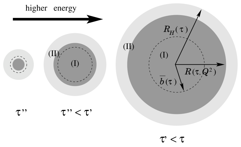
Figure 5: A pictorial representation of the expansion of the black disk with increasing rapidity. The dotted line circle of radius $\bar{b}(\tau)=R_{H}(\tau)/2$ separates between domains (I) and (II).

The evolution of the black disk with increasing $\tau$ at fixed $Q^{2}$ is pictorially illustrated in Fig. 5. The black disk appears at the center of the hadron at a critical rapidity $\bar{\tau}_{1}(Q^{2})$ such that $Q_{s}^{2}(\bar{\tau}_{1},b=0)=Q^{2}$. This condition together with eq. (4.8) implies:

$$\bar{\tau}_{1}(Q^{2})\,=\,\frac{1}{c\bar{\alpha}_{s}}\,\ln\frac{Q^{2}}{\Lambda^{2}}\,.$$ (4.24)

For $\tau>\bar{\tau}_{1}(Q^{2})$, but not much larger, the black disk remains confined to domain (I), as illustrated by the smallest disk on the left of Fig. 5. However, the expansion rate of the black disk, which is equal to $c\lambda_{s}\approx 3.12$ in appropiate units (cf. eq. (4.22)), is faster than the corresponding rate $\omega/2\approx 1.39$ for the borderline $\bar{b}(\tau)\equiv R_{H}(\tau)/2$ between the two domains. Thus, at some new, larger, critical value, which can be easily estimated from eq. (4.22) as

$$\bar{\tau}_{2}(Q^{2})\,=\,\frac{1}{(c-\omega/2\lambda_{s})\bar{\alpha}_{s}}\,\ln\frac{Q^{2}}{\Lambda^{2}}\,,$$ (4.25)

the black disk reaches domain (II), and than extends further within this domain (as illustrated by the two larger disks in Fig. 5). But within domain (II), the expansion rate of the black disk slows down to $\omega\approx 2.77$, cf. eq. (4.10), which is the same rate as for the hadron outer border $R_{H}(\tau)$. Thus, with increasing $\tau$, the radial distance between the border of the black disk and the edge of the hadron (i.e., the width of the grey area) remains constant (cf. eq. (4.11)), so the relative size of the grey area with respect to the hadron size is smaller and smaller (cf. eq. (4.23)). At large $\tau$, this grey area represents the tail of the hadron wavefunction, in which the BFKL equation remains valid even at arbitrarily large energy.

Given the (quasi)exponential decrease of the saturation scale $Q_{s}^{2}(\tau,b)$ with $b$, it is straightforward to verify that the conditions $\Lambda^{2}\ll Q_{s}^{2}(\tau,b)\ll Q^{2}$ hold at any point $b_{\perp}$ in the corona $R(\tau,Q^{2})\ll b_{\perp}\ll R_{H}(\tau)$, as necessary for the consistency of our approximations. Indeed, these conditions are satisfied as soon as the separation between $b_{\perp}$ and the (inner or outer) edges of this corona is of order $1/m_{\pi}$ or larger. For instance, eq. (4.20) can be rewritten as:

$$Q_{s}^{2}(\tau,b)\,\simeq\,\Lambda^{2}\,{\rm e}^{4m_{\pi}(R_{H}(\tau)-b)}\,.$$ (4.26)

Similarly, by using eq. (2.10), the expressions (4.18) and (4.20) can be recast into the form:

$$Q_{s}^{2}(\tau,b)\,\simeq\,Q^{2}\,{\rm e}^{-2\gamma m_{\pi}(b-R(\tau,Q^{2}))}\,,$$ (4.27)

where $\gamma\approx 1.55$ if $b_{\perp}$ is in domain (I), and $\gamma=2$ for $b_{\perp}$ in domain (II).

5 Geometric scaling at high energy

“Geometric scaling” refers to the property of the dipole-hadron total cross section $\sigma(\tau,Q^{2})$, eq. (2.5), to depend upon the two kinematical variables $\tau$ and $Q^{2}$ only via the combination $Q^{2}_{0}(\tau)/Q^{2}$ (the “scaling variable”) where $Q^{2}_{0}(\tau)$ is some suitable momentum scale which increases as a power of the energy: $Q^{2}_{0}(\tau)\propto{\rm e}^{\lambda\tau}$. This property is interesting since it can be related to a similar property of the virtual photon total cross section $\sigma_{\gamma^{*}p}({\rm x},Q^{2})$ which is actually seen in the HERA data on deep inelastic scattering (for ${\rm x}<0.01$ and $Q^{2}<400~{}{\rm GeV}^{2}$) [38].

Clearly, this property cannot hold for arbitrary $\tau$ and $Q^{2}$, since it is known to be violated by the solutions to the linear evolution equations (DGLAP or BFKL) at very high $Q^{2}$. On the other hand, in the saturation regime at $Q^{2}<Q_{s}^{2}(\tau)$, this property is physically motivated, since the saturation scale is then the only scale in the problem [20] (at least for a homogeneous hadron), so it is tempting to identify it with the momentum scale $Q^{2}_{0}(\tau)$ introduced above.

So far, studies of geometric scaling have been performed only for a homogeneous hadron, so they have naturally focused on the corresponding property of the scattering amplitude ${\cal N}_{\tau}(Q^{2})$ (because $\sigma(\tau,Q^{2})=2\pi R^{2}{\cal N}_{\tau}(Q^{2})$ in this case). Such previous studies — which relied on either numerical [32, 23, 39], or (approximate) analytic [29, 30] solutions to the BK equation — not only confirmed the existence of geometric scaling in the saturation regime, but also showed that this property extends up to momenta $Q^{2}$ considerably larger than $Q_{s}^{2}(\tau)$. In particular, in Ref. [29], the upper limit for “extended scaling” has been estimated as $Q^{2}_{max}\sim Q_{s}^{4}(\tau)/\Lambda^{2}$, which is roughly consistent with the phenomenology [38] (see also below).

Our purpose in this section is to extend the analysis of Ref. [29] by taking into account the transverse inhomogeneity in the hadron, within the formalism developed in the previous sections of this paper. Note that, since the impact parameter is integrated over in the formula (2.5) for $\sigma(\tau,Q^{2})$, the connection between the scaling properties of the cross-section and those of the scattering amplitude ${\cal N}_{\tau}(r_{\perp},b_{\perp})$ becomes more subtle now. In particular, it is not a priori clear what should be the scale which plays the role of $Q^{2}_{0}(\tau)$ in the scaling variable, or even whether geometric scaling exists at all (since the inhomogeneous problem is not a single-scale problem any longer).

To progressively introduce the effects of the inhomogeneity, let us start with a situation where the rapidity $\tau$ is small enough for the hadron to look “grey” everywhere: $Q^{2}>Q_{s}^{2}(\tau,b=0)$, or $\tau<\bar{\tau}_{1}(Q^{2})$, cf. eq. (4.24). In that case, and within the present approximations, the scattering amplitude ${\cal N}_{\tau}(Q^{2},b_{\perp})$ is factorized at any $b_{\perp}$ : ${\cal N}_{\tau}(Q^{2},b_{\perp})\simeq{\cal N}_{\tau}(Q^{2})S(b_{\perp})$. Thus, the study of the scaling properties of the total cross-section:

$$\sigma(\tau,Q^{2})\,\simeq\,2{\cal N}_{\tau}(Q^{2})\int d^{2}b_{\perp}\,S(b_{\perp})\qquad({\rm all\,\,grey}),$$ (5.1)

reduces to the corresponding study of ${\cal N}_{\tau}(Q^{2})$ in the homogeneous case [29]. It is instructive to briefly rederive here the main result in Ref. [29] (in a very schematic way):

The homogeneous scattering amplitude ${\cal N}_{\tau}(Q^{2})$ is given by (4.5) with $b=0$. As such, this formula shows no scaling. To see the scaling emerging, we shall replace the arbitrary reference scale $\Lambda^{2}$ in this equation with the saturation scale $Q_{s}^{2}(\tau)=\Lambda^{2}{\rm e}^{c\bar{\alpha}_{s}\tau}$ (which is the same as the central saturation scale $Q_{s}^{2}(\tau,b=0)$ in the inhomogeneous case; cf. eq. (4.8)). We write:

$$\ln\frac{Q^{2}}{\Lambda^{2}}\,=\,\ln\frac{Q^{2}}{Q_{s}^{2}(\tau)}\,+\,\ln\frac{Q_{s}^{2}(\tau)}{\Lambda^{2}}\,=\,\ln\frac{Q^{2}}{Q_{s}^{2}(\tau)}+\,c\bar{\alpha}_{s}\tau\,.$$ (5.2)

Since, by construction, the saturation scale is such that the exponent in (4.5) (with $b=0$) vanishes for ${Q^{2}}={Q_{s}^{2}(\tau)}$, it is clear that, after the replacement (5.2), we are left only with terms involving, at least, one power of $\ln({Q^{2}}/{Q_{s}^{2}(\tau)})$ :

$${\cal N}_{\tau}(Q^{2})\,=\,\exp\left\{-\lambda_{s}\ln\frac{Q^{2}}{Q_{s}^{2}(\tau)}-\frac{1}{2\beta\bar{\alpha}_{s}\tau}\left(\ln\frac{Q^{2}}{Q_{s}^{2}(\tau)}\right)^{2}\right\}.$$ (5.3)

Here, $\lambda_{s}\approx 0.64$ has been generated as $\lambda_{s}=1/2+c/\beta$ (cf. eqs. (4.7) and (4.17)). So far, (5.3) is just a rewriting of eq. (4.5). But this is suggestive of the conditions under which geometric scaling should be expected: This emerges when the (central) saturation scale $Q_{s}^{2}(\tau)$ is sufficiently close to $Q^{2}$ (although still smaller than it) for the quadratic term in eq. (5.3) to be negligible compared to the linear term. When this happens, eq. (5.3) can be approximated as:

$${\cal N}_{\tau}(Q^{2}) \simeq \left(\frac{Q_{s}^{2}(\tau)}{Q^{2}}\right)^{\lambda_{s}}$$ (5.4)

which shows geometric scaling indeed, with $Q_{0}^{2}(\tau)\equiv Q_{s}^{2}(\tau)$. This is valid as long as:

$$1\,<\,\ln\frac{Q^{2}}{Q_{s}^{2}(\tau)}\,\ll\,2\lambda_{s}\beta\bar{\alpha}_{s}\tau,$$ (5.5)

where the lower limit is simply the condition that we are in a regime where eq. (5.1) applies: the hadron looks “grey” everywhere. Since $2\lambda_{s}\beta\approx 43.37$ is a large number, eq. (5.5) gives a rather large window, which however extends beyond the validity range of the BFKL saddle point (4.3) [29]. A more complete analysis [29] shows that eq. (5.5) should be replaced by:

$$1\,<\,\ln\frac{Q^{2}}{Q_{s}^{2}(\tau)}\,<\,\ln\frac{Q_{s}^{2}(\tau)}{\Lambda^{2}}\,=\,c\bar{\alpha}_{s}\tau\,,$$ (5.6)

which for the present purposes is rewritten as a range for $\tau$:

$$\frac{1}{2c\bar{\alpha}_{s}}\ln\frac{Q^{2}}{\Lambda^{2}}\,<\,\tau\,<\,\frac{1}{c\bar{\alpha}_{s}}\ln\frac{Q^{2}}{\Lambda^{2}}\,.$$ (5.7)

The lower limit in the equation above, which arises from the upper limit in eq. (5.6), is the smallest value of $\tau$ at which the BFKL solution starts to behave like a scaling function, for a given $Q^{2}$. As for the upper limit — in which we recognize the critical value $\bar{\tau}_{1}(Q^{2})$ for the emergence of the black disk, eq. (4.24) —, this is necessary only for the validity of eq. (5.1). For higher values of $\tau$, geometric scaling may still hold, but in order to see it, the calculation should be modified to account for the formation of the black disk.

Specifically, for $\tau>\bar{\tau}_{1}(Q^{2})$, the cross-section (2.5) can be then decomposed into a “black” contribution plus a “grey” one, which are evaluated as (for $R(\tau,Q^{2})>1/m_{\pi}$):

$$\sigma(\tau,Q^{2}) \simeq 2\pi R^{2}(\tau,Q^{2})\,+\,2{\cal N}_{\tau}(Q^{2})\int d^{2}b_{\perp}\,S(b_{\perp})\,\Theta(b-R(\tau,Q^{2}))$$ (5.8)

$$\simeq 2\pi R^{2}(\tau,Q^{2})\,+\,\frac{2\pi R(\tau,Q^{2})}{m_{\pi}}\,.$$

The second line is obtained from the first one after replacing $S(b)\approx{\rm e}^{-2m_{\pi}b}$, and noticing that ${\cal N}_{\tau}(Q^{2}){\rm e}^{-2m_{\pi}R(\tau,Q^{2})}=1$. Eq. (5.8) confirms that, when the energy is large enough for $R(\tau,Q^{2})>1/m_{\pi}$, the total cross-section is dominated by the black disk, as anticipated in Sect. 2. It further shows that the scaling properties of the cross section are determined by the corresponding properties of the radius of the black disk, which can be inferred from the discussion in Sect. 4. As in Sects. 4.3–4.4, we are led to distinguish between two regimes:

I) If $\bar{\tau}_{1}(Q^{2})<\tau<\bar{\tau}_{2}(Q^{2})$, cf. eqs. (4.24)–(4.25), the black disk lies entirely inside domain (I), and the corresponding radius is given by eq. (4.22), which is now rewritten as :

$$R(\tau,Q^{2})\Big{|}_{(I)}\,\simeq\,\frac{\lambda_{s}}{2m_{\pi}}\ln\frac{Q_{s}^{2}(\tau,b=0)}{Q^{2}}\,.$$ (5.9)

This shows scaling, with the same scaling variable $Q^{2}_{s}(\tau)/Q^{2}$ as in the “all grey” regime (5.7).

II) In the high-energy regime $\tau>\bar{\tau}_{2}(Q^{2})$, the edge of the black disk is in domain (II), so its radius is given by eq. (4.10). This shows scaling too, but with a different scaling variable:

$$R(\tau,Q^{2})\Big{|}_{(II)}\,=\,\frac{1}{4m_{\pi}}\ln\frac{Q^{2}_{\infty}(\tau)}{Q^{2}},\qquad Q^{2}_{\infty}(\tau)\equiv\Lambda^{2}{\rm e}^{2\omega\bar{\alpha}_{s}\tau}.$$ (5.10)

This gives the scaling law for the total cross section at very high energy:

$$\sigma(\tau,Q^{2})\simeq 2\pi R^{2}(\tau,Q^{2})=\frac{\pi}{2m_{\pi}^{2}}\left(\ln\frac{Q^{2}_{\infty}(\tau)}{Q^{2}}\right)^{2}\,.$$ (5.11)

To summarize, for fixed $Q^{2}$ and intermediate energies corresponding to the following range of rapidities (cf. eqs. (5.7) and (4.25)):

$$\frac{1}{2c\bar{\alpha}_{s}}\ln\frac{Q^{2}}{\Lambda^{2}}\,<\,\tau\,<\,\frac{1}{(c-\omega/2\lambda_{s})\bar{\alpha}_{s}}\,\ln\frac{Q^{2}}{\Lambda^{2}}\,=\,\bar{\tau}_{2}(Q^{2})\,,$$ (5.12)

the dipole-hadron cross-section exhibits geometric scaling, with the scale set by the central saturation scale $Q^{2}_{s}(\tau)\equiv Q^{2}_{s}(\tau,b=0)$. Eq. (5.12) allows for a significant window since, numerically, $2c\approx 9.68$ while $c-\omega/2\lambda_{s}\approx 2.69$. On the other hand, at higher energies, corresponding to $\tau>\bar{\tau}_{2}(Q^{2})$, there is scaling again, but the relevant scale is rather the asymptotic scale $Q^{2}_{\infty}(\tau)$.

Of course, the scaling breaks down, strictly speaking, for $\tau\sim\bar{\tau}_{2}(Q^{2})$, i.e., in the transition regime where the black disk crosses from domain (I) to domain (II). But it so happens that, numerically, the difference between the exponents $c\approx 4.84$ and $2\omega\approx 5.55$ in the corresponding scaling variables ($Q^{2}_{s}(\tau)$ and, respectively, $Q^{2}_{\infty}(\tau)$) is quite small, so the transition from one scaling law to the other takes places rather fast, as also manifest in the plot in Fig. 4.

It should be also stressed that, with incresing $\tau$, the geometric scaling becomes less and less relevant, since the $Q^{2}$–dependence of the cross-section (5.11) eventually becomes a subleading effect: When the condition (4.2) is fulfilled, the leading-order term in eq. (5.11) is simply proportional to $\tau^{2}$, with the scale set by the pion mass (cf. eq. (2.17)).

For completness, let us conclude with a discussion of the scaling properties of the local scattering amplitude ${\cal N}_{\tau}(Q^{2},b_{\perp})$. Within the grey area, the factorization property ${\cal N}_{\tau}(Q^{2},b_{\perp})=S(b_{\perp}){\cal N}_{\tau}(Q^{2})$ implies that any scaling property of the homogeneous solution ${\cal N}_{\tau}(Q^{2})$ transmits automatically to ${\cal N}_{\tau}(Q^{2},b_{\perp})$, but with a scaling variable involving the local saturation scale $Q_{s}^{2}(\tau,b)$ :

$${\cal N}_{\tau}(Q^{2})\,=\,\left(\frac{Q_{0}^{2}(\tau)}{Q^{2}}\right)^{\lambda}\,\longrightarrow\,\,\,{\cal N}_{\tau}(Q^{2},b_{\perp})\,=\,\left(\frac{Q_{s}^{2}(\tau,b)}{Q^{2}}\right)^{\lambda}\,,$$ (5.13)

with $Q_{s}^{2}(\tau,b)=Q_{0}^{2}(\tau){\rm e}^{-2m_{\pi}b/\lambda}$. This is precisely the scaling solution (3.11) that we used in our arguments in Sect. 3.1. In eq. (5.13), the momentum scale $Q_{0}^{2}(\tau)$ and the power $\lambda$ depend upon the rapidity $\tau$, in the expected way: When $\tau$ is in the intermediate range (5.12), $Q_{0}^{2}(\tau)$ is the saturation scale at the center $Q_{s}^{2}(\tau,b=0)$, and $\lambda=\lambda_{s}\approx 0.64$. At higher rapidities, $\tau>\bar{\tau}_{2}(Q^{2})$, one rather has $Q_{0}^{2}(\tau)=Q^{2}_{\infty}(\tau)$ and $\lambda=1/2$.

In both cases, eq. (5.13) holds only in the grey area at $b>R(\tau,Q^{2})$. But inside the black disk, geometric scaling holds as well, and almost trivially, since there ${\cal N}_{\tau}(Q^{2},b_{\perp})\approx 1$ and the deviation from one shows scaling too [32, 22, 29]. We thus conclude that, for any $\tau$ above the lower limit in eq. (5.7), the scattering amplitude ${\cal N}_{\tau}(Q^{2},b_{\perp})$ shows geometric scaling everywhere in the hadron disk.

6 Conclusions and outlook

In this paper, we have proposed a simple mechanism combining perturbative gluon saturation and non-perturbative boundary conditions which ensures the saturation of the Froissart bound in dipole-hadron scattering at high energy. Gluon saturation has been implemented via the non-linear evolution equations derived in perturbation theory in Refs. [7, 8, 9, 10], that we have used only for impact parameters in the central region of the hadron, where the gluon density is high and perturbation theory is applicable. On the basis of these equations, we have shown that, with increasing energy, the non-linear effects ensure not only the unitarization of the scattering amplitude at fixed impact parameter, but also the factorization of the impact parameter dependence of the scattering amplitude in the outer “grey area”, where the unitarity limit has not yet been reached. This factorization, together with the exponential fall-off of the non-perturbative initial condition at large distances, leads to a total cross-section which grows like $\ln^{2}s$. The coefficient of this growth is universal, i.e., independent of the hadronic target, and has been computed here.

Our analysis makes explicit the deep connection between unitarization effects and the formation of the Colour Glass Condensate. The “black disk” within which the unitarity limit has been reached is precisely the region of the hadron where the gluons “seen” by the incoming dipole are saturated, whereas the “grey area” corresponds to a region of lower density, in which the BFKL evolution still applies. The transition from “grey” to “black”, i.e., the expansion of the black disk, is described by the non-linear evolution equations for the Colour Glass Condensate. The colour correlations at saturation are essential for both factorization and unitarization: They ensure colour neutrality for the saturated gluons, and thus suppress the non-unitary contributions due to the long-range Coulomb tails.

We have given the first computation of the saturation scale for an inhomogeneous hadron and identified two factorization regimes at different impact parameters. This has interesting consequences for the geometric scaling properties of the total cross-section: Our analysis predicts two different scaling laws in different ranges of energy.

For simplicity, our analysis has been carried out for an external probe which is a $q\bar{q}$ dipole of fixed transverse size. But its extension to deep inelastic scattering should be straightforward. To this aim, the dipole-hadron cross-section must be averaged over all transverse sizes of the $q\bar{q}$ pair, with a weight given by the light-cone wavefunction of the virtual photon [24, 25, 26].

It is important to point out two limitations of our approach, which call for further studies. First, it was essential for our approximation scheme that the dipole is small, $r_{\perp}\ll 1/\Lambda_{QCD}$. In particular, this restricts the applicability of our results to deep inelastic scattering at relatively large photon virtuality, $Q^{2}\gg\Lambda_{QCD}^{2}$. It would be most interesting to see if one can phenomenologically extend this analysis towards the strong coupling regime at $Q^{2}\sim\Lambda_{QCD}^{2}$ using the ”soft pomeron”, and thus get at least an estimate for the coefficient of the $\ln^{2}s$ growth in that regime.

Second, we have performed our analysis at fixed coupling. It is an interesting open question how our results would be modified by the running of the coupling. Strictly speaking, this running is one of the next-to-leading order effects which so far have not been systematically included in the non-linear evolution equations (see, however, [40]). But the experience with the BFKL equation, for which the NLO corrections have been recently computed [41], suggests that a significant part of these corrections could be indeed taken into account by including the running of the coupling. Then, the natural question is, what should be the scale at which the coupling must be evaluated.

In a previous paper [29], where the saturation scale $Q_{s}(\tau)$ for a homogeneous hadron has been computed, we found it natural to evaluate the coupling at the saturation momentum. Indeed, in that problem, the rapidity $\tau$ and the external momentum $Q^{2}$ (the resolution of the dipole) were increased simultaneously, in such a way to preserve the saturation condition $Q_{s}^{2}(\tau)=Q^{2}$. For that particular running, we have shown that the saturation momentum changes its parametric dependence upon rapidity with respect to the fixed coupling case, from ${\rm e}^{c\alpha_{s}\tau}$ to ${\rm e}^{\kappa\sqrt{\tau+\tau_{0}}}$ (with constant $\kappa$ and $\tau_{0}$). This result has been subsequently confirmed in Ref. [30].

On the other hand, in the present paper the physical situation is quite different: The external momentum $Q^{2}$ is fixed, and with increasig $\tau$, we simultaneously increase the impact parameter $b$, in such a way that the condition $Q_{s}^{2}(\tau,b)=Q^{2}$ (which defines the edge of the black disk) remains satisfied. It seems therefore natural to evaluate the coupling at the fixed external scale $Q^{2}$, in which case the fixed coupling expressions obtained in this paper would remain valid (after the trivial replacement $\alpha_{s}\to\alpha_{s}(Q^{2})$). A further argument in this sense is provided by the discussion in Sect. 3.1, which shows that the dominant scattering involves only nearby colour sources, within the area covered by the incoming dipole or slightly further away, so that the typical transferred momenta are of order $Q^{2}$.

A still different possibility for the running, which would be closer in spirit to Ref. [29], would be to evaluate the coupling at the local saturation scale $Q_{s}^{2}(\tau,b)$. Although this scale and the external scale $Q^{2}$ are identified at the edge of the black disk, they are nevertheless different at the points $b_{\perp}$ which lie further away in the grey area (where $Q^{2}\gg Q_{s}^{2}(\tau,b)$). Thus, this choice for the running would probably modify the current formulae, in such a way to provide a generalization of the results in Ref. [29] to the case of an inhomogeneous hadron.

Of course, the description above is extremely crude and exploratory, and a full analysis of the running coupling case is required before any strong conclusions can be drawn.

Note added

After the submission of the original version of this paper, there appeared a preprint by Kovner and Wiedemann which disputes the claims of this paper [42]. In Sec. 3.2, we have added some clarifying comments which we hope will ameliorate this dispute. In this note, we would like to discuss this in more detail.

We are first of all pleased to notice that the authors of Ref. [42] have to some extent agreed with our criticism to their papers [14], and modified their arguments accordingly. For instance, they now agree that the dominant contribution to the scattering within the “grey area” comes from local sources (although their exact definition of the “grey area” is somewhat different from ours). Also, they admit that the long-range, non-unitary, contribution to the scattering amplitude that they previously computed in Ref. [14] applies only for a coloured probe, and not for a dipole.

But in spite of their agreement on these points, the authors of Ref. [42] dispute our conclusion on “Froissart bound from gluon saturation”, and instead conclude that the Froissart bound is violated by the perturbative evolution equations in Refs. [7, 8, 9, 10]. In its essence (but using the language of our Sect. 3.2), the argument of Ref. [42] can be formulated as follows: Assume that one starts the perturbative evolution at some early rapidity $\tau_{0}$, at which the point $b_{\perp}$ of interest lies far outside the initial “grey area” ($b\gg R_{H}(\tau_{0})$), i.e., in the “white area”, according to the terminology of Ref. [42]. In this perturbative setting, the dominant contribution to the scattering amplitude at $b_{\perp}$ is the long-range contribution, which decreases only as $1/b_{\perp}^{4}$, cf. eq. (3.34). With increasing $\tau$, the central region expands, and the point $b_{\perp}$ is eventually incorporated in the “grey area” at some “time” $\tau_{1}$. For $\tau>\tau_{1}$, the evolution proceeds locally at $b_{\perp}$, but with an initial condition at $\tau=\tau_{1}$ which decreases as a power of $b_{\perp}$, rather than as an exponential. Thus, the first term in the r.h.s. of eq. (3.34) is replaced by ${\rm e}^{\omega\bar{\alpha}_{s}\tau}/b_{\perp}^{4}$, and the “blackness” condition ${\cal N}_{\tau}(r_{\perp},b_{\perp})\sim 1$ yields a black disk increasing exponentially with $\tau$.

Although mathematically correct (at least, in its above formulation; we disagree with some of the intermediate steps and detail points in Ref. [42]), this argument is physically irrelevant: It simply signals a pathology of perturbation theory when this is used in a region where it is not supposed to work, namely, in the “white area”, where physics is truly controlled by the confinement. In the discussion in Sect. 3.2, we pointed out that, under plausible assumptions about the non-perturbative physics in this region, the true evolution respects the exponential fall-off of the initial condition.

In any case, our point in this paper was not to argue that, by integrating the perturbative evolution up to arbitrarily large $\tau$, one would generate cross-sections which saturate the Froissart bound indefinitely. Rather, we have shown that by applying perturbation theory where it is expected to work — namely, in the central region at $b<R_{H}(\tau)$, where the condition $Q_{s}(\tau,b)\gg\Lambda_{QCD}$ is satisfied by definition (cf. eq. (2.12)) —, one finds that (i ) it is possible to compute the expansion rate of the black disk, and (ii ) this rate is such that the Froissart bound is saturated. None of these points is trivial:

(i ) It was not a priori obvious that the expansion of the black disk is controlled by perturbation theory. We have demonstrated this for the case of a small dipole ($Q^{2}\gg\Lambda_{QCD}^{2}$), for which we have shown that the “grey area” ($\equiv$ the region in which $Q_{s}^{2}(\tau,b)$ decreases from $Q^{2}$ down to $\Lambda_{QCD}^{2}$) has a considerable extent (cf. eq. (4.11)). This is the region which controls the expansion, and perturbation theory is applicable here.

(ii ) It was not a priori clear that the perturbative evolution of the black disk will respect the Froissart bound. Indeed, the saturated gluons from the black disk generate long-range forces which remain perturbative at impact parameters within the “grey area”, and thus cannot be discarded by invoking confinement. (This was precisely the objection to Froissart bound raised in Ref. [14].) We have shown that these long-range forces, although present, are nevertheless harmless: Because the saturated gluons are globally colour-neutral (an aspect which has been overlooked in Ref. [14]), they generate only dipolar forces, whose contribution to the scattering amplitude in the grey area remains smaller than the corresponding contribution of the local sources (which saturates the Froissart bound).

The only place where non-perturbative physics has entered our argument was in providing the $b_{\perp}$–dependence of the initial condition for the short-range contribution. On physical grounds, this is fixed by confinement, and thus is certainly of the exponential type (and not of the power-law type, as a naïve perturbative evolution starting in the “white area” would predict).

To conclude, Kovner and Wiedemann seem to be addressing a different question: Whether or not one can naïvely apply the perturbative evolution equation in all regions of impact parameter space — including over distances many times the pion Compton wavelength —, and still get sensible results. They negatively answer this question, and we definitely agree with them on this point. On the other hand, they further make the statement that one cannot compute the high-energy cross section using the ideas associated with (perturbative) saturation. The body of this paper clearly contradicts this claim.

References

- [1] J.R. Cudell et al, Phys. Rev. D65 (2002) 074024.
- [2] M. Froissart, Phys. Rev. 123 (1961) 1053.
- [3] Y.S. Jin and A. Martin, Phys. Rev. 135 (1964) B 1375; A. Martin, Nuovo Cimento 42 (1966) 930.
- [4] L. Lukaszuk and A. Martin, Nuovo Cimento A52 (1967) 122.
- [5] W. Heisenberg, Z. Phys. 133 (1952) 65.
- [6] A. Hebecker, “Non-perturbative high-energy QCD,” hep-ph/0111092.
- [7] I. Balitsky, Nucl. Phys. B463 (1996) 99; High-energy QCD and Wilson lines, hep-ph/0101042, in “At the Frontier of Particle Physics / Handbook of QCD”. Edited by M. Shifman, World Scientific, Singapore, 2001.
- [8] Yu.V. Kovchegov, Phys. Rev. D60 (1999) 034008; ibid. D61 (2000) 074018.
- [9] H. Weigert, Nucl. Phys. A703 (2002) 823.
- [10] E. Iancu, A. Leonidov and L. McLerran, Nucl. Phys. A692 (2001), 583; Phys. Lett. B510 (2001) 133; E. Ferreiro, E. Iancu, A. Leonidov and L. McLerran, Nucl. Phys. A703 (2002) 489.
- [11] E.M. Levin and M.G. Ryskin, Phys. Rept. 189 (1990) 267.
- [12] L.V. Gribov, E.M. Levin, and M.G. Ryskin, Phys. Rept. 100 (1983) 1.
- [13] A.H. Mueller and J. Qiu, Nucl. Phys. B268 (1986) 427.
- [14] A. Kovner and U.A. Wiedemann, Nonlinear QCD Evolution: Saturation without Unitarization, hep-ph/0112140; Perturbative Saturation and the Soft Pomeron, hep-ph/0204277.
- [15] L.N. Lipatov, Sov. J. Nucl. Phys. 23 (1976) 338; E.A. Kuraev, L.N. Lipatov and V.S. Fadin, Zh. Eksp. Teor. Fiz 72, 3 (1977) (Sov. Phys. JETP 45 (1977) 199); Ya.Ya. Balitsky and L.N. Lipatov, Sov. J. Nucl. Phys. 28 (1978) 822.
- [16] M. Braun, Eur. Phys. J. C16 (2000) 337.
- [17] A. H. Mueller, Phys. Lett. B523 (2001) 243.
- [18] E. Iancu, A. Leonidov and L. McLerran, The Colour Glass Condensate: An Introduction, hep-ph/0202270. Lectures given at the NATO Advanced Study Institute “QCD perspectives on hot and dense matter”, August 6–18, 2001, Cargèse, France.
- [19] A. H. Mueller, Parton Saturation-An Overview, Cargese lectures, Lectures given at Cargese Summer School on QCD Perspectives on Hot and Dense Matter, Cargese, France, 6-18 August 2001, hep-ph/0111244.
- [20] L. McLerran and R. Venugopalan, Phys. Rev. D49 (1994) 2233; ibid. 49 (1994) 3352; ibid. 50 (1994) 2225.
- [21] A.H. Mueller, Nucl. Phys. B558 (1999) 285.
- [22] E. Iancu and L. McLerran, Phys. Lett. B510 (2001) 145.
- [23] K. Golec-Biernat, L. Motyka, and A.M. Staśto, Phys. Rev. D65 (2002) 074037.
- [24] A.H. Mueller, Nucl. Phys. B335 (1990) 115.
- [25] A.H. Mueller, Nucl. Phys. B415 (1994) 373; ibid. B437 (1995) 107.
- [26] N.N. Nikolaev and B.G. Zakharov, Z. Phys. C49 (1991) 607, ibid. C53 (1992) 331.
- [27] W. Buchmuller, M.F. McDermott and A. Hebecker, Nucl. Phys. B487 (1997) 283, Erratum-ibid. B500 (1997) 621; W. Buchmuller, T. Gehrmann, and A. Hebecker Nucl. Phys. B537 (1999) 477.
- [28] H. Fujii and D. Kharzeev, Phys. Rev. D60, (1999) 114039.
- [29] E. Iancu, K. Itakura, and L. McLerran, Geometric Scaling above the Saturation Scale, hep-ph/0203137, to appear in Nucl. Phys. A.
- [30] A. H. Mueller and D. N. Triantafyllopoulos, The energy dependence of the saturation momentum, hep-ph/0205167.
- [31] V.N. Gribov and L.N. Lipatov, Sov. Journ. Nucl. Phys. 15 (1972) 438; G. Altarelli and G. Parisi, Nucl. Phys. B126 (1977) 298; Yu. L. Dokshitzer, Sov. Phys. JETP 46 (1977) 641. See also Yu. L. Dokshitzer, V. A. Khoze, A.H. Mueller, and S.I. Troyan, “Basics of Perturbative QCD” (Editions Frontières, Gif-sur-Yvette, 1991).
- [32] E. Levin and K. Tuchin, Nucl. Phys. B573 (2000) 833; Nucl. Phys. A691 (2001) 779; Nucl. Phys. A693 (2001) 787.
- [33] N. Armesto and M. Braun, Eur. Phys. J. C20 (2001) 517; ibid. C22 (2001) 351.
- [34] J. Jalilian-Marian, A. Kovner, A. Leonidov and H. Weigert, Nucl. Phys. B504 (1997) 415; Phys. Rev. D59 (1999) 014014.
- [35] A.L. Ayala, M.B. Gay Ducati, and E.M. Levin, Phys. Lett. B388 (1996) 188.
- [36] M. Lublinsky, E. Gotsman, E. Levin, and U. Maor, Nucl. Phys. A696 (2001) 851.
- [37] A.J. Askew, J. Kwieciński, A.D. Martin, and P.J. Sutton, Phys. Rev. D49 (1994) 4402.
- [38] A.M. Staśto, K. Golec-Biernat, and J. Kwieciński, Phys. Rev. Lett. 86 (2001) 596.
- [39] M. Lublinsky, Eur. Phys. J. C21 (2001) 513.
- [40] I. Balitsky and A.V. Belitsky, Nucl. Phys. B629 (2002) 290.
- [41] V.S. Fadin and L.N. Lipatov, Phys. Lett. B429 (1998) 127; G. Camici and M. Ciafaloni, Phys. Lett. B430 (1998) 349.
- [42] A. Kovner and U.A. Wiedemann, No Froissart Bound from Gluon Saturation, hep-ph/0207335.