Precision Electroweak Tests of the Standard Model

Abstract

The present status of precision electroweak data is reviewed. These data include measurements of $\mathrm{e}^{+}\mathrm{e}^{-}\rightarrow{\rm f}\overline{\rm f}$, taken at the Z resonance at LEP, which are used to determine the mass and width of the ${\mathrm{Z}}$ boson. In addition, measurements have also been made of the forward-backward asymmetries for leptons and heavy quarks, and also the final state polarisation of the $\tau$-lepton. At SLAC, where the electron beam was polarised, measurements were made of the left-right polarised asymmetry, $A_{\rm{LR}}$, and the left-right forward-backward asymmetries for b and c quarks.

The mass, $m_{\mathrm{W}}$, and width, $\Gamma_{\mathrm{W}}$, of the W boson have been measured at the Tevatron and at LEP, and the mass of the top quark, $m_{\mathrm{t}}$, has been measured at the Tevatron. These data, plus other electroweak data, are used in global electroweak fits in which various Standard Model parameters are determined. A comparison is made between the results of the direct measurements of $m_{\mathrm{W}}$ and $m_{\mathrm{t}}$ with the indirect results coming from electroweak radiative corrections. Using all precision electroweak data fits are also made to determine limits on the mass of the Higgs boson, $m_{\mathrm{H}}$. The influence on these limits of specific measurements, particularly those which are somewhat inconsistent with the Standard Model, is explored. The data are also analysed in terms of the quasi model-independent $\epsilon$ variables.

Finally, the impact on the electroweak fits of the improvements in the determination of the W-boson and top-quark masses, expected from the Tevatron Run 2, is examined.

• † Denys Wilkinson Building, Keble Road, Oxford OX1 3RH

  e-mail p.renton1@physics.ox.ac.uk

to be published in Reports on Progress in Physics

1 Introduction

The Standard Model (SM) has not come from a sudden inspirational flash of brilliance, be it in the bath or elsewhere! Instead it is a compact summary of experimental facts and theoretical ideas. It has taken the painstaking work of many thousands of researchers, both experimenters and theorists, over several decades to achieve the form of the model that we know today. Apart from a few possible discrepancies, which are discussed in detail below, the model is consistent with a huge amount of precisely measured physical quantities. The various pieces of data which have, from time to time, shown conflict with the SM have, on analysing more (or better quality) data, returned to the fold of compatibility with the SM.

Yet the Standard Model is almost certainly wrong! It is clearly incomplete, as it does not include the force of gravity. It also suffers from severe theoretical problems when the higher-order perturbative corrections to the Higgs boson mass are computed. These corrections would most naturally be infinite in the SM, and can only be rendered finite by rather inelegant means. The introduction of Supersymmetry, in which a supersymmetric partner for each SM particle is introduced, can cure the potential divergences associated with the Higgs particle. However, the cost is a large increase in the number of parameters in the model. As yet, there is no direct evidence for Supersymmetry.

This review is organised as follows. In section 2 a brief review of the Standard Model is given, together with a discussion of electroweak radiative corrections. The properties and results of the Z boson are described in section 3, and those of the W boson in section 4. In section 5, the running of the electromagnetic coupling constant $\alpha$(s) is discussed, and in section 6 other electroweak measurements are briefly described. In section 7 the constraints and tests of the validity of the Standard Model are examined, and in section 8 the future prospects for electroweak measurements are assessed. There is a brief summary in section 9.

2 The Standard Model

2.1 The building blocks

In the development of the Standard Model experimental discovery and theoretical insights have gone hand in hand. Experimentally, the discovery of the electron, then the nucleus and its proton and neutron constituents, was the starting point. Studies on radioactive nuclei led to the recognition that, in addition to electromagnetic interactions, there were also weak interactions, and to the hypothesis of the feebly interacting neutrino. The experimental discovery of a more massive lepton, the muon, was (and still is) a puzzle. The third charged lepton, the $\tau$, completes the known spectrum. In addition, it was experimentally established that the neutrinos associated with the electron and the muon have different interactions. Our current picture is that we have three generations of leptons: the electron, muon and tau, and their corresponding neutrinos. These neutrinos are light on the scale of the charged leptons, and there is an increasing body of experimental evidence, from neutrino-oscillation experiments, indicating that one or more may have non-zero mass.

The discovery of the pion, followed by the kaon and many other meson and baryon states, manifested the strong interaction. The study of the lowest-lying meson and baryon multiplets led to the hypothesis of non-integrally charged up(u), down(d) and strange(s) quarks. Initially the quark-model was regarded by many as a convenient classification scheme for hadronic states, without the quarks necessarily having any physical significance. The extension of this static quark idea to a more physical dynamic interpretation came as a result of studies of deep-inelastic scattering off nucleons, using both charged lepton and neutrino beams. At high enough energies, the scattering was consistent with being off the fractionally charged up and down quark constituents of the nucleon. These results also suggested, by energy-momentum conservation, that there was a further fundamental constituent of the nucleon, the gluon, which did not participate directly in these interactions. Studies of the process $\mathrm{e}^{+}\mathrm{e}^{-}\rightarrow{\rm q}\overline{\rm q}$ had shown that hadronic jets were formed along the directions of the quark and antiquarks, giving a two jet topology in the bulk of the events. The study of three-jet events showed the existence of the process $\mathrm{e}^{+}\mathrm{e}^{-}\rightarrow{\rm q}\overline{\rm q}{\rm g}$, in which the gluon produced a jet of hadrons similar in properties to those produced by quarks and antiquarks.

Various experimental observations involving quarks, together with the symmetry principles of the wave-functions of the lightest baryons, led to the concept of colour; that is, each quark comes in three distinct types, or colours. This, plus further work on these strong interactions and the discovery of charm(c), bottom(b) and top(t) quarks, led to the formulation of the theory of Quantum Chromodynamics (QCD), which attempts to describe the strongly interacting behaviour of quarks, antiquarks and gluons.

Pioneering work, post Second World War, showed that the potentially infinite quantities in Quantum Electrodynamics (QED), such as the mass and charge of the electron, could be controlled through the procedure of renormalisation. This renewed attempts to produce a combined description of electromagnetic and weak interactions in terms of a relativistic quantum field theory. The existing theory of weak interactions at that time was the V-A theory, which grew out of Fermi’s theory. In the V-A theory the fermions have only left-handed couplings. These ideas could be extended to include a virtual massive charged vector boson W, with a role analogous to that of the photon in QED, but the resulting theory was not renormalisable. A crucial piece of experimental input was the discovery of neutral currents (NC) in neutrino-nucleon deep inelastic scattering. Prior to this, charged current (CC) interactions had been found, which could be described by the exchange of a virtual charged W boson, leading to a final state containing a charged lepton. In the neutral current interactions there was no final state charged lepton, and this indicated the exchange of a massive neutral boson, the Z boson.

Further work has also shown that the six quarks can be grouped into three doublets u-d, c-s and t-b. This grouping is similar to that of the three left-handed lepton doublets, each of which consists of a neutrino and its corresponding charged lepton. There is an underlying SU(2) symmetry, and the quantum number corresponding to these doublets is called weak isospin; in analogy with the strong isospin successfully developed in understanding strong interactions. The leptons and quarks also have right-handed singlet states corresponding to a U(1) symmetry, with quantum number weak hypercharge.

The unified electroweak theory which evolved, and which was later shown to be renormalisable, described the interactions of the spin-$\frac{1}{2}$ fermions (leptons and quarks) and the spin-1 gauge bosons (photon, Z and W^+-). To describe the neutral current interactions, the physical photon (A⁰) and Z boson (Z⁰) fields are written as a linear combination of the neutral gauge bosons W${}^{0}_{3}$ and B, which correspond to the SU(2) and U(1) groups respectively, as follows

$$Z^{0}=\cos\theta_{W}W^{0}_{3}-\sin\theta_{W}B^{0}$$

$$A^{0}=\sin\theta_{W}W^{0}_{3}+\cos\theta_{W}B^{0},$$ (1)

where $\theta_{W}$ is the Weinberg or weak mixing angle.

This theory, due mainly to Glashow, Salam and Weinberg, unified the weak and electromagnetic forces, but with just these spin-$\frac{1}{2}$ fermions and spin-1 bosons all the particles in this theory are massless. The W and Z bosons have masses of about $m_{\mathrm{W}}\simeq$80 GeV and $m_{\mathrm{Z}}\simeq$ 91 GeV respectively, whereas the direct experimental limit on the photon mass is m${}_{\gamma}\leq$ 2 10^-16 eV [2], and is consistent with being massless. A massless gauge boson is described by only two spin states, whereas there are three for the massive case. A possible remedy was provided by the introduction of a complex weak doublet of scalar bosons, the Higgs doublet, which gives mass to the fermions and the massive gauge bosons. Through the process of spontaneous local symmetry breaking three members of the Higgs doublet gets ‘eaten’ to form the longitudinal spin states of the massive gauge bosons. This leaves one massive physical neutral scalar particle, the Higgs boson H. This Higgs mechanism gives the relationship that $m_{\mathrm{W}}$ = $m_{\mathrm{Z}}$$\cos\theta_{W}$, or $\sin^{2}\!\theta_{\mathrm{W}}=1-m_{\mathrm{W}}^{2}/m_{\mathrm{Z}}^{2}$, between the masses of the W and Z bosons. These massive gauge bosons were discovered in high energy proton-antiproton collisions at CERN. The mass of the Higgs boson is not predicted by the theory, and so far it has not been discovered. There is, however, a possible signal, with a significance of about 2 standard deviations, from the combined LEP data, at a mass of 115 GeV [3].

The fermion masses are accounted for by introducing a fermion-Higgs field with Yukawa couplings. This does the job, but there is no predictive power on the fermion masses since each mass corresponds to an arbitrary coupling parameter, and must therefore be specified from the experimentally measured value.

For the strong interaction sector of the SM, invariance under local colour transformations leads to the theory of QCD and the group SU(3)_c. The gauge bosons are the eight massless gluons.

2.2 Electroweak interactions

The charged fermions have both left-handed and right-handed states. The electromagnetic interaction depends only on the charge of the fermion and does not distinguish between these states. However, the weak interaction does depend on the handedness of the state. For example, for the first generation of leptons, the left-handed electron state $\rm{e}_{\rm L}$ and the neutrino $\nu_{\rm e}$ form a weak isospin doublet, whereas the right-handed state $\rm{e}_{\rm R}$ is a singlet. In addition to the left-handed weak isospin t, there is a further quantum number, the weak hypercharge y; defined such that the charge q = t₃ + y/2. The properties of the fundamental fermions are given in table 1. Note that the classification for neutrinos is that of the Minimal Standard Model, in which the neutrinos are massless.

Table 1: Quantum numbers for the fermions in the Standard Model, where q is the charge, and $t$ and $t_{3}$ denote the weak isospin and its third component.

• Fermion Generation				Quantum Numbers
  1	2	3	$q$	$t$	$t_{3}$
  Leptons
  $\left(\begin{array}[]{c}\nu_{\rm e}\\ e\end{array}\right)_{L}$	$\left(\begin{array}[]{c}\nu_{\mu}\\ \mu\end{array}\right)_{L}$	$\left(\begin{array}[]{r}\nu_{\tau}\\ \tau\end{array}\right)_{L}$	$\begin{array}[]{c}0\\ -1\end{array}$	$\frac{1}{2}$	$\begin{array}[]{c}+\frac{1}{2}\\ -\frac{1}{2}\end{array}$
  $e_{R}$	$\mu_{R}$	$\tau_{R}$	$-1$	$0$	$0$
  Quarks
  $\left(\begin{array}[]{c}u\\ d\end{array}\right)_{L}$	$\left(\begin{array}[]{c}c\\ s\end{array}\right)_{L}$	$\left(\begin{array}[]{c}t\\ b\end{array}\right)_{L}$	$\begin{array}[]{c}+\frac{2}{3}\\ -\frac{1}{3}\end{array}$	$\frac{1}{2}$	$\begin{array}[]{c}+\frac{1}{2}\\ -\frac{1}{2}\end{array}$
  $u_{R}$	$c_{R}$	$t_{R}$	$+\frac{2}{3}$	$0$	$0$
  $d_{R}$	$s_{R}$	$b_{R}$	$-\frac{1}{3}$	$0$	$0$

The electroweak theory is based on the symmetry of invariance under local gauge transformations. That is, the physical equations are invariant under a phase change applied independently at each space-time point. The group corresponding to weak isospin is SU(2)_L, whereas that for weak hypercharge is U(1)_y. In the electroweak theory there is invariance under SU(2)${}_{\rm L}\otimes$U(1)_y. There are constants g and g${}^{{}^{\prime}}$ corresponding to the SU(2)_L and U(1)_y groups. These are related to the electron charge e and $\sin\theta_{\mathrm{W}}$ by

$$e=g\sin\theta_{\mathrm{W}}=g^{{}^{\prime}}\cos\theta_{\mathrm{W}}.$$ (2)

2.3 Electroweak couplings of SM particles

The interaction vertices involving a Vector Boson (V=W,Z) and a fermion-antifermion pair (see fig.1) are of great importance. These can be classified as charged or neutral currents, depending on the nature of the Vector Boson.

Figure 1: The interaction vertex of a Vector Boson V (W or Z) with a fermion-antifermion pair.

Charged current interactions involve the W^+- bosons, and the interaction Lagrangian for the W${\mathrm{f}\bar{f}^{{}^{\prime}}}$ vertex has the form

$${\cal L}_{CC}=-\frac{g}{2\sqrt{2}}W_{\mu}^{-}j^{\mu}_{CC},$$ (3)

with

$$j^{\mu}_{CC}=\bar{f^{{}^{\prime}}}\gamma^{\mu}(1-\gamma^{5})f,$$ (4)

where (f,${\mathrm{\bar{}}{f}^{{}^{\prime}}}$) = ($\ell^{-}$,$\bar{\nu_{\ell}}$) for leptons and ($q_{\frac{1}{3}}$,$\bar{q_{\frac{2}{3}}}$) for quarks, with $q_{\frac{1}{3}}$ = (d,s,b) and $q_{\frac{2}{3}}$ = (u,c,t). This form corresponds to pure left-handed coupling of the W to fermions.

The neutral current Lagrangian for the Z${\rm f}\overline{\rm f}$ vertex can be written as

$${\cal L}_{NC}^{Z}=-\frac{g}{2\cos\theta_{\mathrm{W}}}Z_{\mu}j^{\mu}_{NC},$$ (5)

with

$$j^{\mu}_{NC}=\bar{f}\gamma^{\mu}(v_{\rm{f}}-a_{\rm{f}}\gamma^{5})f=\bar{f}\gamma^{\mu}[C_{L}^{f}(1-\gamma^{5})+C_{R}^{f}(1+\gamma^{5})]f.$$ (6)

Here $v_{\rm{f}}$ and $a_{\rm{f}}$ are the vector- and axial-vector couplings. There are both left-handed (C${}_{L}^{f}=\ell_{f}=(v_{\rm{f}}+a_{\rm{f}})/2$) and right-handed (C${}_{R}^{f}$ = r_f = ($v_{\rm{f}}-a_{\rm{f}})/2$) terms. In the SM, at tree-level,

$$v_{\rm{f}}=t^{3}_{\rm f}-2q_{\rm f}\sin^{2}\!\theta_{\mathrm{W}},\hskip 28.45274pta_{\rm{f}}=t^{3}_{\rm f},$$ (7)

where t${}_{f}^{3}$ is the third component of the weak-isospin (see tab.1).

The photon-fermion coupling, for a fermion of charge q_f, has the form

$${\cal L}_{NC}^{\gamma}=-eq_{f}A_{\mu}j^{\mu}_{\gamma},\\$$

with

$$j^{\mu}_{\gamma}=\bar{f}\gamma^{\mu}f,$$ (8)

that is, the left- and right-handed couplings are equal, and there is only a vector term. For the case of polarised fermions, the left- and right-handed fermion components, i.e. (1-$\gamma^{5}$) and (1+$\gamma^{5}$), are used. More details and specific Born-level calculations in the SM can be found in [1].

Many of the electroweak interactions discussed later involve the scattering of two fermions i.e. f₁f${}_{2}\rightarrow$ f₃f₄. The matrix element for this process has the form

$${\cal M}_{fi}\propto j_{12}^{\mu}(P_{V})_{\mu\nu}j_{34}^{\nu},$$ (9)

with j${}_{12}^{\mu}$ = $\bar{f_{2}}\gamma^{\mu}(\epsilon_{V}-\epsilon_{A}\gamma^{5})f_{1}$ etc. The couplings $\epsilon_{V}$ and $\epsilon_{A}$ depend on the form of the interaction, as discussed above. The vector-boson propagator P_V has the form 1/s for a photon, and the relativistic Breit-Wigner resonance form

$$P_{V}\propto\frac{1}{s-M_{V}^{2}+is\Gamma_{V}/M_{V}}$$ (10)

for V=W or Z, where s is the centre-of-mass energy squared. For the case of a neutral current interaction involving charged particles, both $\gamma$ and Z exchange are possible, so there is a $\gamma$-Z interference term. This latter term has an energy dependence proportional to the difference (s-$m_{\mathrm{Z}}^{2}$), and so changes sign in going from below to above the Z-pole. The fermion decay f${}_{1}\rightarrow$ f₂f₃f₄ has a CC matrix element similar in form to that in eqn.(9), with a W-boson far from its mass shell except for the decay of the top-quark.

The Higgs boson is a neutral scalar particle in the SM, of (unknown) mass $m_{\mathrm{H}}$. In the kinematic regime explored at LEP the main decays considered are H $\rightarrow{\rm f}\overline{\rm f}$. The coupling is proportional to the fermion mass m_f, so H $\rightarrow{\mathrm{b}\overline{\mathrm{b}}}$ and H $\rightarrow\tau^{+}\tau^{-}$ are the dominant decay modes for $m_{\mathrm{H}}$ up to about 120 GeV. For higher masses the decays H $\rightarrow$ WW and ZZ become increasingly important.

2.4 Parameters and predictions of the SM

In the Standard Model there is invariance under the combination SU(3)${}_{\rm c}\otimes$SU(2)${}_{\rm L}\otimes$U(1)_y. The Lagrangian of the Standard Model can be completely specified, but exact solutions have so far not been obtained. Instead, low-order perturbation theory is used. The infinities arising in the renormalisation process are rendered harmless by expressing the results of these perturbative calculations in terms of precisely known physical quantities.

The QCD part of the SM, corresponding to the SU(3)_c group, has only one parameter: the gauge coupling constant g_s. This constant is not specified by the theory. Higher order QCD effects introduce a dependence on the momentum scale Q in the QCD coupling parameter $\alpha_{\rm S}$. The value of $\alpha_{\rm S}$(Q) decreases as the scale Q increases. It is usual to specify the value at the scale Q = $m_{\mathrm{Z}}$; thus giving $\alpha_{\rm S}$($m_{\mathrm{Z}}$).

The electroweak sector is more complicated. There are constants g and g${}^{{}^{\prime}}$ corresponding to the SU(2)_L and U(1)_y groups. The Higgs potential term in ${\cal L}_{\rm SM}$ is

$$V(\phi)=\mu^{2}\mid\phi\mid^{2}+\lambda^{2}\mid\phi\mid^{4},$$ (11)

with parameters $\mu$ ($\mu^{2}<$ 0) and $\lambda$. Alternatively these can be cast in terms of the vacuum expectation value (vev), $v$, and the mass of the Higgs boson, $m_{\mathrm{H}}$.

There are also parameters associated with the masses and mixing angles of the leptons and quarks. For the lepton sector, in the case of massless neutrinos, there are three parameters corresponding to the charged lepton masses. For the quark sector there are parameters for the quark masses, and there are four mixing angles needed to describe the CC transitions between quark states. The set of these fermion parameters is referred to as $\{\rm{m_{f}}\}$. This gives in total 17 parameters for the electroweak sector, and all but two of these (g and g${}^{{}^{\prime}}$) are associated with the Higgs field. The number of parameters is of course larger if the neutrino sector also has mass. Thus the Higgs can solve the problem of giving mass to the particles, but only at the expense of a large number of parameters.

In addition, the SM embodies some explicit assumptions which do not directly appear as parameters. The hypothesis of lepton universality is assumed. That is, the overall couplings of the leptons are the same, and any differences arise only from the lepton masses. The same is also the case with the quark sector. It is thus important to test these hypotheses experimentally.

In addition to the aesthetic problem that the Higgs mechanism introduces a large number of parameters, there is a further, and more fundamental, problem with the Higgs boson. The mass of the scalar Higgs boson has contributions from loop diagrams which involve integration over the four-momentum of the loop. The resulting Higgs mass depends on the upper limit of this integration. In the SM there is no upper scale to fix this limit. The SM does not include the force of gravity, which is another serious deficiency. Using the Planck scale of $\simeq$ 10¹⁹ GeV as an upper limit could resolve the problem, but only at the expense of having to fine-tune cancellations to many significant figures. The problem of the large difference between the electroweak scale and that where new physics, beyond the SM, enters is known as the hierachy or naturalness problem.

A possible solution to the hierachy problem is the introduction of a further symmetry of nature called supersymmetry. This corresponds to space-time transformations which change fermions into bosons, and vice versa. The introduction of supersymmetry (or SUSY) essentially doubles the number of fundamental particles. There is a scalar super-partner for each fermion and a spin-$\frac{1}{2}$ super-partner for each spin-1 particle. In the calculation of the Higgs mass, the loop contributions from the s-particles have the opposite sign to those of their corresponding particles, and thus tend to cancel the divergent loop contributions. However, none of these super-particles (or s-particles) have been observed, so supersymmetry, and this cancellation, cannot be exact. For the cancellation to work, the s-particles cannot be too massive; and that sets an upper limit on the s-particle masses in the TeV range.

The introduction of supersymmetry into the SM, the simplest version of which is the Minimal Supersymmetric Standard Model (MSSM), brings with it many (more than 100) extra prameters. There is, without as yet any experimental guidance, a choice among many possibilities as to how supersymmetry is broken. The phenomenology is thus complicated and is outside the scope of this article.

2.5 Electroweak Radiative Corrections

In the electroweak sector, as discussed above, there are the SM parameters g and g${}^{{}^{\prime}}$, or e and $\sin^{2}\!\theta_{\mathrm{W}}$, as well as the Higgs mass $m_{\mathrm{H}}$ and vev $v$. Alternatively, these can be expressed in terms of the electromagnetic coupling constant $\alpha$, the gauge boson masses $m_{\mathrm{Z}}$ and $m_{\mathrm{W}}$, and also $m_{\mathrm{H}}$. In addition, there are the fermion parameters $\{\rm{m_{f}}\}$, and the QCD parameter $\alpha_{\rm s}$.

For SM predictions at the scale $m_{\mathrm{Z}}$, the QED coupling, $\alpha$, is needed at this scale. Although $\alpha(0)$, at scale q² = 0, is precisely known experimentally, there is, as discussed in section 5, some significant uncertainty on $\alpha(m_{\mathrm{Z}})$. The value of the Fermi coupling constant, $G_{\mathrm{F}}$, is accurately determined from measurements of $\mu$ decays [2]. Although $G_{\mathrm{F}}$ is specified directly in terms of $m_{\mathrm{W}}$ at the Born-level, the introduction of higher-order loops means that, in the calculation of $m_{\mathrm{W}}$ in terms of $G_{\mathrm{F}}$, a dependence on other SM parameters enters the computation.

The relationship between the neutral and charged weak couplings fixes the ratio of the W and Z boson masses, namely

$$\rho=\frac{m_{\mathrm{W}}^{2}}{m_{\mathrm{Z}}^{2}\cos^{2}\!\theta_{\mathrm{W}}}.$$ (12)

This $\rho$ parameter is determined by the Higgs structure of the theory. In the Minimal Standard Model, where there are only Higgs doublets, $\rho$ is unity. Electroweak radiative corrections lead to $\rho$ = 1 + $\Delta\rho$.

Electroweak corrections modify the tree-level relationships such that

$$G_{\mathrm{F}}=\frac{\pi\alpha}{\sqrt{2}m_{\mathrm{W}}^{2}\sin^{2}\!\theta_{\mathrm{W}}}\frac{1}{(1-\Delta{r})},$$ (13)

where $\sin^{2}\!\theta_{\mathrm{W}}=1-m_{\mathrm{W}}^{2}/m_{\mathrm{Z}}^{2}$. The quantity $\Delta{r}$, which is zero at tree-level, is given by

$$\Delta{r}=\Delta\alpha+\Delta{r}_{\mathrm{w}}.$$ (14)

The term $\Delta\alpha$ controls the running of $\alpha$(s), and is given by

$$\alpha(s)=\frac{\alpha(0)}{1-\Delta\alpha(s)}=\frac{\alpha(0)}{1-\Delta\alpha_{lept}(s)-\Delta\alpha_{top}(s)-\Delta\alpha^{(5)}_{had}(s)},$$ (15)

where $\alpha$(0) = 1/137.036. At LEP/SLD energy scales this becomes $\alpha(m_{\mathrm{Z}})\simeq$ 1/129. The dominant term in $\Delta{r}_{\mathrm{w}}$ is given by $\Delta\rho$, defined above:

$$\Delta{r}_{\mathrm{w}}=-\frac{\cos^{2}\!\theta_{\mathrm{W}}}{\sin^{2}\!\theta_{\mathrm{W}}}\Delta\rho+\Delta{r}_{\mathrm{remainder}}.$$ (16)

Figure 2: Electroweak loop corrections to the gauge boson propagators.

Electroweak corrections enter through loop diagrams to the vector boson propagators, see fig.2, and through vertex corrections. The leading-order contributions to $\Delta{r}_{\mathrm{w}}$ depend on the masses of the top quark, $m_{\mathrm{t}}$ and Higgs boson, $m_{\mathrm{H}}$:

$$\Delta{r}^{\mathrm{t}} = -\frac{3G_{\mathrm{F}}m_{\mathrm{W}}^{2}}{8\sqrt{2}\pi^{2}}\frac{m_{\mathrm{t}}^{2}}{m_{\mathrm{W}}^{2}}\frac{\cos^{2}\!\theta_{\mathrm{W}}}{\sin^{2}\!\theta_{\mathrm{W}}}+\cdots$$ (17)

$$\Delta{r}^{\mathrm{H}} = \frac{11}{3}\frac{G_{\mathrm{F}}m_{\mathrm{W}}^{2}}{8\sqrt{2}\pi^{2}}\left(\ln\frac{m_{\mathrm{H}}^{2}}{m_{\mathrm{W}}^{2}}-\frac{5}{6}\right)+\cdots.$$ (18)

The leading contributions are thus $\Delta{r}^{\mathrm{t}}\propto m_{\mathrm{t}}^{2}$ and $\Delta{r}^{\mathrm{H}}\propto\ln(m_{\mathrm{H}})$. The largest effect is from the top-quark mass, $m_{\mathrm{t}}$. This is because of the large difference in mass between $m_{\mathrm{t}}$ ($\simeq$ 175 GeV) and that of the bottom-quark, $m_{\mathrm{b}}$ ($\simeq$ 5 GeV).

The large amount of electroweak data, accumulated from $\mathrm{e}^{+}\mathrm{e}^{-}$ colliders working at the Z peak and available in the early Nineties, was sufficiently accurate to make an estimate of the top-quark mass from electroweak fits, within the context of the SM. For example, the data available in Summer 1994 [5], around the time of the top-quark discovery, gave $m_{\mathrm{t}}$ = 173 ${}^{+12}_{-13}$ GeV for $m_{\mathrm{H}}$ = 300 GeV, with additional uncertainties of -20 and +18 GeV if the Higgs mass is varied from 60 to 1000 GeV. This SM prediction was in good agreement with the directly measured value of $m_{\mathrm{t}}\simeq$ 175 GeV. This represents a triumph for the Standard Model. The current situation, and also the sensitivity to the Higgs boson mass, is discussed in section 7.

A more detailed discussion of electroweak radiative corrections, as well as other theoretical issues of the SM, can be found in [6, 7].

3 The Z boson

The data on the Z boson discussed in this review come from the $\mathrm{e}^{+}\mathrm{e}^{-}$ colliders at LEP in CERN, Geneva, Switzerland, and from the Stanford Linear Collider (SLC), in California, USA. Most of the Z boson data are, or are very close to being, final. The data used here are mainly those presented at the EPS 2001 Conference in Budapest, Hungary, in July 2001 [8], in which a full list of references to individual results can be found.

The lowest-order Feynman diagrams for the process $\mathrm{e}^{+}\mathrm{e}^{-}\rightarrow\mu^{+}\mu^{-}$, and also where there is an initial state radiation of a photon, are shown in fig. 3.

Figure 3: Feynman diagrams for the lowest-order process $\mathrm{e}^{+}\mathrm{e}^{-}\rightarrow\mu^{+}\mu^{-}$ and for the case where there is initial state radiation of a photon.

3.1 Z boson variables

The Z boson decays to $\mathrm{f}\bar{\mathrm{f}}$ and the $\mathrm{{Z}f\overline{f}}$ vertex can be described by effective vector ($v_{\rm{f}}$) and axial-vector ($a_{\rm{f}}$) coupling constants  such that, to a very good approximation, the Born-level formulae are retained. It is useful to define the polarisation parameter

$$\mbox{$\cal A_{\rm f}$}=\frac{2v_{\rm{f}}a_{\rm{f}}}{(v_{\rm{f}}^{2}+a_{\rm{f}}^{2})}=\frac{\ell_{f}^{2}-r_{f}^{2}}{\ell_{f}^{2}+r_{f}^{2}}\ \ .$$ (19)

The cross-section for $\mathrm{e}^{+}\mathrm{e}^{-}\rightarrow{\rm f}\overline{\rm f}$, close to the ${\mathrm{Z}}$ pole, may be written in terms of the Z mass, $m_{\mathrm{Z}}$, and total width, $\Gamma_{\mathrm{Z}}$, as

$$\sigma_{f}(s)=\frac{\sigma_{f}^{0}}{(1+\delta_{\rm QED})}\frac{s\Gamma_{\mathrm{Z}}^{2}}{(s-m_{\mathrm{Z}}^{2})^{2}+s^{2}\Gamma_{\mathrm{Z}}^{2}/m_{\mathrm{Z}}^{2}}\hskip 14.22636pt+\sigma_{\gamma}+\sigma_{\gamma/\mbox{${\mathrm{Z}}$}}\ ,$$ (20)

where s is the square of the $centre-of-mass$ energy. The QED factor $\delta_{\rm QED}$ = 3$\alpha(m_{\mathrm{Z}})$/4$\pi$ cancels the corresponding factor in the ${\Gamma_{\rm e\overline{\rm e}}}$ partial width (see below). The contributions $\sigma_{\gamma}$ and $\sigma_{\gamma/\mbox{${\mathrm{Z}}$}}$ from $\gamma$-exchange and $\gamma$-Z interference are small ($\mathbin{\mskip 5.0mu plus 5.0mu\raise 1.0pt\hbox{$<$}\kern-8.0pt\lower 3.0pt\hbox{$\sim$}\mskip 5.0mu plus 5.0mu}$1$\%$) in the region around the Z-pole. The Breit-Wigner form has an s-dependent width, which takes into account higher-order effects [9]. $\sigma_{f}^{0}$ is the pole cross-section, which is defined as

$$\sigma_{f}^{0}=\frac{12\pi{{\Gamma_{\rm e\overline{\rm e}}}{\Gamma_{{\rm f}\overline{\rm f}}}}}{m_{\mathrm{Z}}^{2}\Gamma_{\mathrm{Z}}^{2}}.$$ (21)

Here, ${\Gamma_{{\rm f}\overline{\rm f}}}$ is the partial width for $\mathrm{{Z}\rightarrow f\overline{f}}$, which in turn can be written as

$${\Gamma_{{\rm f}\overline{\rm f}}}=\frac{G_{\mathrm{F}}m_{\mathrm{Z}}^{3}}{6\pi\sqrt{2}}(v_{\rm{f}}^{2}+a_{\rm{f}}^{2})f_{QCD}f_{QED}\ \ .$$ (22)

The final-state QED correction factor is f_QED = 1 + 3$\alpha(m_{\mathrm{Z}})$Q${}_{f}^{2}$/4$\pi$, whereas f_QCD is unity for leptons and f_QCD = 3(1 + c${}_{q}\alpha_{\rm{s}}{\rm(m_{\mathrm{Z}})}/\pi$ + ..) for quarks, with c${}_{q}\simeq$ 1.

The formula for the cross-section $\sigma_{f}$(s) is an effective Born-level formula and must be convoluted with QED radiative corrections before comparing with experiment. The cross-sections which are measured in practice are for $\mathrm{e}^{+}\mathrm{e}^{-}\rightarrow\mathrm{hadrons}$ and $\mathrm{e}^{+}\mathrm{e}^{-}\rightarrow\ell^{+}\ell^{-}$, for $\ell$ = e,$\mu$,$\tau$. The hadronic width $\Gamma_{\mathrm{had}}$ is the sum of $\Gamma_{q}$ for q=u,d,s,c,b. The total Z width, assuming lepton universality, is $\Gamma_{\mathrm{Z}}=\Gamma_{\mathrm{had}}+3{\Gamma_{\ell\overline{\ell}}}+\Gamma_{\mathrm{inv}}$, where $\Gamma_{\mathrm{inv}}=3\Gamma_{\nu\overline{\nu}}$ in the SM. The results below are expressed in terms of the ratio of the hadronic to leptonic partial widths R_ℓ ($\ell$ = e,$\mu$,$\tau$), where

$$R_{\ell}=\frac{\Gamma_{\mathrm{had}}}{{\Gamma_{\ell\overline{\ell}}}}.$$ (23)

The distribution of the angle $\theta$ of the outgoing fermion f, with respect to the incident e^- direction is given, at Born-level, by

$$\frac{d\sigma}{d\cos\theta}\propto 1+\cos^{2}\theta+\frac{8}{3}A_{\mathrm{FB}}\cos\theta.$$ (24)

The forward-backward asymmetry is defined as $A_{\mathrm{FB}}^{\mathrm{f}}=(\sigma_{\rm F}-\sigma_{\rm B})/(\sigma_{\rm F}+\sigma_{\rm B})$, where $\sigma_{\rm F}$ ($\sigma_{\rm B}$) are the cross-sections in the forward (backward) directions. The value measured at the Z-pole, the pole asymmetry, is defined as

$$A^{0,\,{\rm f}}_{\rm{FB}}=\frac{3}{4}\mbox{$\cal A_{\rm e}$}\mbox{$\cal A_{\rm f}$}\ .$$ (25)

Since $\cal A_{\rm f}$ depends on the ratio $v_{\rm{f}}$/$a_{\rm{f}}$, a measurement of $A^{0,\,{\rm f}}_{\rm{FB}}$ depends on both $v_{\rm{e}}/a_{\rm{e}}$ and $v_{\rm{f}}/a_{\rm{f}}$. The effective couplings can also be written as

$$a_{\rm{f}}=t^{3}_{\rm f}\sqrt{\rho_{\rm f}}\ ,\ \ \ \ \ \frac{v_{\rm{f}}}{a_{\rm{f}}}=1-4|q_{\rm f}|\sin^{2}\!\theta_{\rm{eff}}^{\rm{f}}\ ,$$ (26)

where $t^{3}_{\rm f}$ is the third component of the weak isospin. The mixing angle defined for leptons ($\sin^{2}\!\theta_{\rm{eff}}^{\rm{lept}}$) is used for reference. Those defined for quarks have small shifts, due to SM plus any new physics [10].

3.2 LEP lineshape scans and beam energy determination

The LEP $\mathrm{e}^{+}\mathrm{e}^{-}$ Collider took data at the Z-pole between 1989 and 1995 (LEP 1 phase). There were lineshape scans, in which data were taken at a series of energy settings within $\pm$ 3 GeV of the Z-pole, in all years except 1992 and 1994. The early scans had seven energy points, whereas those in 1993 and 1995 had three points. In the two latter scans, the two off-peak energy points were situated at about 1.8 GeV below and above the ${\mathrm{Z}}$ peak, and are referred to as peak-2 and peak+2 respectively. The choice of these energies optimised the precision on the Z width. In both these scans the total off-peak luminosity was about 20 pb^-1, significantly higher than in the 1991 and earlier scans.

Good accuracy on the LEP beam energy E_LEP is crucial in the determination of $m_{\mathrm{Z}}$ and $\Gamma_{\mathrm{Z}}$. A precise energy calibration measurement (E${}_{LEP}^{pol}$, with $\delta$E${}_{cms}\leq$ 0.8 MeV) of the average circulating beam energy can be made using the technique of resonant depolarisation. This technique was available, but only at one energy point, for the 1991 scan. For the 1993 and 1995 scans it was available at all the energy points. For the two latter scans, most of the energy calibration measurements were performed after physics data-taking at the end of fills. For the 1993 scan, about one-third of the off-peak fills (representing about 40$\%$ of the recorded off-peak luminosity) was calibrated. For the 1995 scan about 70$\%$ of the recorded off-peak luminosity was calibrated.

Although resonant depolarisation gives a very precise energy value at the time of measurement, the LEP energy varies with time, due to the Earth tides and other effects such as the temperature of the dipole magnets. Since the RF frequency, and thus the orbit length, is fixed, stresses in the local rock structure result in changes to the position of the beams in the quadrupole magnets. This changes the beam energy, since the effective dipole field changes. These energy changes can be tracked accurately using measurements of the horizontal beam orbit positions, x_orb. For the 1993 scan a model for E_LEP was developed, based on x_orb, together with correction terms from the magnetic dipole fields and temperatures, the RF cavity voltages, as well as other factors [11].

In the analysis of the 1993 scan a term was included for the increase in the energy during a fill, based on observations of an NMR device in a reference dipole magnet (outside the LEP ring), which showed an upward drift in the field together with occasional jumps of a few MeV. To understand better these effects in 1995, two NMR devices were inserted in dipole magnets in the LEP ring. Furthermore, in four physics fills energy calibration measurements were made at both the beginning and end of fills to measure the energy change. The NMR devices showed a significant amount of noise, which was largely anti-correlated in the two devices which were on opposite sides of the LEP ring, and which was much smaller between midnight and 5am. The main cause of this noise was traced to local electric trains, the earth currents from which travelled along the LEP beam pipe. When averaged over several fills these NMR devices showed an increase in energy during a fill of typically 5 MeV (much larger than the rise estimated in  [11]). The magnitude of the rise was confirmed using the beginning and end of fill energy calibrations, as well as studies of fills in machine development periods in 1993 and 1995 in which energy calibration measurements were made over periods of several hours.

An improved model, including this rise term, was developed [12], both for the 1995 scan and also for a revised analysis of the 1993 scan, and also the 1994 peak data. For each energy and year a single normalisation parameter was used and the rms values of E${}_{LEP}^{model}$ - E${}_{LEP}^{pol}$ were determined. These rms values (typically a few MeV) are of importance in determining the energy error on those fills with no polarisation measurement, since it is assumed that these follow the same distribution. The error for the 1995 scan from this effect is smaller than for 1993 since a much higher fraction of the off-peak luminosity was collected in calibrated fills.

The analysis of the energy values and errors for the years 1993 to 1995 includes estimates of the correlations both between energy points and between years  [12]. The correlations between off-peak energy points are important because error components which are highly correlated do not contribute significantly to $\delta\Gamma_{\mathrm{Z}}$. The contributions of the LEP energy uncertainties to the errors on $m_{\mathrm{Z}}$ and $\Gamma_{\mathrm{Z}}$ are $\delta m_{\mathrm{Z}}$(LEP) $\simeq\pm$ 1.7 MeV and $\delta\Gamma_{\mathrm{Z}}$(LEP) $\simeq\pm$ 1.2 MeV.

The uncertainty of the LEP cms energy spread ($\simeq$ 55 $\pm$ 1 MeV) also gives rise to an error on $\Gamma_{\mathrm{Z}}$, amounting to $\pm$ 0.2 MeV, significantly improved with respect to  [11]. There are also smaller effects on some of the other Z parameters, as detailed below.

3.3 LEP data on cross-sections and lepton asymmetries

Between 1989 and 1995 a total of 15.5 million hadronic ${\mathrm{Z}}$ decays and 1.7 million leptonic decays were recorded by the four LEP experiments (ALEPH, DELPHI, L3 and OPAL). These events have distinctive topologies; for the hadronic events there is a large visible energy and a large hadron multiplicity, whereas for the leptonic events there are two, approximately back-to-back, high energy leptons. Each experiment measures the total cross-section for $\mathrm{e}^{+}\mathrm{e}^{-}\rightarrow\mathrm{hadrons}$ and $\mathrm{e}^{+}\mathrm{e}^{-}\rightarrow\ell^{+}\ell^{-}$ ($\ell$ = e,$\mu$,$\tau$), and the forward-backward asymmetries for $\mathrm{e}^{+}\mathrm{e}^{-}\rightarrow\ell^{+}\ell^{-}$, at each energy point.

The data taking periods can be separated into two phases. In the first phase, up to 1992, the energy determination was rather imprecise. The second phase consisted of data from the 1993 and 1995 scans, and from the $\simeq$ 60 pb^-1 on-peak data in 1994. Details of the analysis methods of the four experiments can be found in  [13, 14, 15, 16].

As discussed below, fits are made to the entire dataset by each experiment, taking into account the correlations in systematic errors arising for experimental effects such as detection efficiencies, the LEP energy uncertainties and also theoretical uncertainties.

To match these impressive statistics the systematic errors need to be well understood. This is indeed the case. The experimental error on the luminosity, which is determined from the $\mathrm{e}^{+}\mathrm{e}^{-}\rightarrow\mathrm{e}^{+}\mathrm{e}^{-}$ cross-section at small angles, is determined to better than 0.1% by each of the four experiments. This requires knowledge of both the absolute and relative positions of the detectors at the 10-20 $\mu$m level; an impressive achievement.

The theoretical error on the luminosity has improved significantly since the 1994 ICHEP in Glasgow [5], when the error was $\delta\cal L/\cal L$(theory) = 0.25%. More recent calculations, using BHLUMI 4.04  [17, 18], include $\cal O$($\alpha^{2}$L²) terms (where L denotes the leading log term), as well as improved treatment of the $\gamma$-Z interference contributions. The estimated theory error is $\delta\cal L/\cal L$(theory) = 0.06%. Note, however, that this error is common between the LEP experiments , and is comparable to that from the combined experimental component, which is also about 0.06%.

The event selection efficiency for $\sigma$($\mathrm{e}^{+}\mathrm{e}^{-}\rightarrow\mathrm{hadrons}$) is known to the very accurate precision of $\mathbin{\mskip 5.0mu plus 5.0mu\raise 1.0pt\hbox{$<$}\kern-8.0pt\lower 3.0pt\hbox{$\sim$}\mskip 5.0mu plus 5.0mu}$ 0.1%. The averages of the measurements of the hadronic cross-sections, as a function of centre-of-mass energy, are shown in fig. 4. The importance of the effects of initial state QED radiative effects can be seen, as the cross-section deconvoluted for these effects is also shown. The lepton cross-section efficiencies are somewhat less well determined (0.1-0.7%), and the systematic errors on these measurements are roughly comparable to the statistical errors. The errors on $A_{\mathrm{FB}}^{\ell}$ are mainly statistical in nature. However, for the reaction $\mathrm{e}^{+}\mathrm{e}^{-}\rightarrow\mathrm{e}^{+}\mathrm{e}^{-}$ there is a large t-channel contribution, and this is subtracted in order to obtain the s-channel cross-sections and asymmetries; see, for example, fig. 5. The theoretical errors estimated for this subtraction [20], which are again common between the experiments, amount to 0.025 nb on $\sigma_{\mathrm{h}}^{0}$, 0.024 on $R_{\mathrm{e}}$ and 0.0014 on $A^{0,\,{\rm e}}_{\rm{FB}}$. The correlation between these, and also the correlations induced because of the uncertainty in $m_{\mathrm{Z}}$ in making these subtractions, are all taken into account.

The forward-backward asymmetries for leptons have also been measured as a function of $\sqrt{s}$. An example of the results is shown in fig. 6.

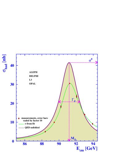
Figure 4: Average LEP hadronic cross-sections, as a function of centre-of-mass energy. The errors have been multiplied by a factor 10 for clarity. The shaded area shows the cross-section, deconvoluted for the effects of QED, which defines the Z parameters discussed in the text.

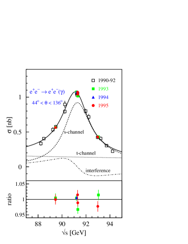
Figure 5: Cross-section for Bhabha scattering, as a function of cms energy, from the L3 Collaboration, showing the s,t and s-t interference components.

Figure 6: Forward-backward asymmetry for $\mathrm{e}^{+}\mathrm{e}^{-}\rightarrow\mu^{+}\mu^{-}$, as a function of cms energy, from the OPAL experiment.

3.4 Combining the LEP lineshape and asymmetries

The combination of the data from the four LEP experiments should, ideally, take place at the level of the measured observable quantities: the cross-sections and asymmetries. However, due to the very complicated nature of the correlations, this has not been attempted. Instead, for the purposes of combining the LEP data, each experiment provides the results of a (so-called) model-independent fit to their cross-section and asymmetry data in terms of nine variables. These are chosen to have small experimental correlations and are $m_{\mathrm{Z}}$, $\Gamma_{\mathrm{Z}}$, $\sigma_{\mathrm{h}}^{0}$, $R_{\ell}$ and $A^{0,\,\ell}_{\rm{FB}}$ ($\ell$ = e,$\mu$,$\tau$). These so-called pseudo-observables or POs, as defined in  [7], have been shown to represent the results from each experiment, which consist of around 200 cross-section and asymmetry measurements, to an excellent degree of precision. The results of a 9 parameter fit to the combined LEP data are given in table 2.

The combination takes into account errors which are common between the experiments. These are shown in table 3. Those arising from the uncertainty on the LEP energy determination and the beam energy spread, the t-channel subtraction and the theoretical uncertainty on the luminosity have already been discussed. More details can be found in  [21], where the full correlation matrices are also given.

The remaining error in table 3, the ‘theory’ error, covers the effects of QED uncertainties and differences in the precision electroweak programs (TOPAZ0 [22], ZFITTER [23] and MIZA [24]), used to extract the pseudo-observables.

Uncertainties in the QED corrections, both from the effects of uncalculated higher-order terms and from initial state fermion pair radiation, have been evaluated. Initial state radiation corrections to ${\cal O}(\alpha^{3})$  [25, 26, 27] (and see also  [28, 29, 30, 31, 32, 33, 34] for earlier work) are included, and a comparison of the predictions of TOPAZ0 and ZFITTER [22, 23] has been made to evaluate the fermion pair uncertainties. The resulting uncertainties are estimated to be 0.3 and 0.2 MeV on $m_{\mathrm{Z}}$ and $\Gamma_{\mathrm{Z}}$ respectively, and 0.02% on $\sigma_{\mathrm{h}}^{0}$.

A comparison of the theoretical predictions for the cross-sections of the programs TOPAZ0 and ZFITTER, for a given set of SM input parameters, has been performed [22, 23, 35]. These differences have been transformed into differences in the fitted POs. The uncertainties estimated in this way are 0.1 MeV on both $m_{\mathrm{Z}}$ and $\Gamma_{\mathrm{Z}}$, 0.001nb on $\sigma_{\mathrm{h}}^{0}$, 0.004 on $R_{\ell}$ and 0.0001 on $A^{0,\,\ell}_{\rm{FB}}$.

The largest uncertainty arising from the parameterisation used in extracting the POs is from the $\gamma$-Z interference term for the $\mathrm{e}^{+}\mathrm{e}^{-}\rightarrow{\rm q}\overline{\rm q}$ channel, which is fixed to its SM value. Changing the Higgs mass from 100 and 1000 GeV, gives a change of +0.23 MeV on $m_{\mathrm{Z}}$. The uncertainty in $\alpha(m_{\mathrm{Z}})$ (see section 5) leads to a negligible change in $m_{\mathrm{Z}}$. The effects on the other POs are also negligible.

If lepton universality is imposed (evidence for this is discussed below), then there are five variables. The results of the fit to the combined LEP data are given in table 4. It can be seen from tables 2 and  4 that the Z mass and width are determined to $\delta m_{\mathrm{Z}}$= 2.1 MeV and $\delta\Gamma_{\mathrm{Z}}$= 2.3 MeV respectively. These are impressive accuracies.

As a cross-check of the LEP energy determination, the values of $m_{\mathrm{Z}}$ for three separate periods of data taking, namely the early data up to 1992, and the 1993 and 1995 energy scans, have been determined. The values measured for these three periods are $m_{\mathrm{Z}}$ = 91.1904 $\pm$ 0.0065, $m_{\mathrm{Z}}$ = 91.1882 $\pm$ 0.0033 and $m_{\mathrm{Z}}$ = 91.1866 $\pm$ 0.0024 GeV respectively, giving confidence in the LEP energy determination.

Table 2: Results and correlation matrix of the 9 parameter fit to the LEP data. The $\chi^{2}$/df of the average is 33/27, a probability of 21%.

quantity	value	error	$m_{\mathrm{Z}}$	$\Gamma_{\mathrm{Z}}$	$\sigma_{\mathrm{h}}^{0}$	$R_{\mathrm{e}}$	$R_{\mu}$	$R_{\tau}$	$A^{0,\,{\rm e}}_{\rm{FB}}$	$A^{0,\,\mu}_{\rm{FB}}$	$A^{0,\,\tau}_{\rm{FB}}$
$m_{\mathrm{Z}}$(GeV)	91.1876	0.0021	1.000	-0.024	-0.044	0.078	0.000	0.002	-0.014	0.046	0.035
$\Gamma_{\mathrm{Z}}$(GeV)	2.4952	0.0023		1.00	-0.297	-0.011	0.008	0.006	0.007	0.002	0.001
$\sigma_{\mathrm{h}}^{0}$(nb)	41.541	0.037			1.00	0.105	0.131	0.092	0.001	0.003	0.002
$R_{\mathrm{e}}$	20.804	0.050				1.00	0.069	0.046	-0.371	0.020	0.013
$R_{\mu}$	20.785	0.033					1.00	0.069	0.001	0.012	-0.003
$R_{\tau}$	20.764	0.045						1.00	0.003	0.001	0.009
$A^{0,\,{\rm e}}_{\rm{FB}}$	0.0145	0.0025							1.00	-0.024	-0.020
$A^{0,\,\mu}_{\rm{FB}}$	0.0169	0.0013								1.00	0.046
$A^{0,\,\tau}_{\rm{FB}}$	0.0188	0.0017									1.00

Table 3: Total and common systematic error components for the 9 parameters.

• quantity	total error	LEP energy	t-chann.	luminosity	theory
  $\delta m_{\mathrm{Z}}$(MeV)	2.1	1.7	-	-	0.3
  $\delta\Gamma_{\mathrm{Z}}$(MeV)	2.3	1.2	-	-	0.2
  $\delta\sigma_{\mathrm{h}}^{0}$(nb)	0.037	0.011	-	0.025	0.008
  $\delta R_{\mathrm{e}}$	0.050	0.013	0.024	-	0.004
  $\delta R_{\mu}$	0.033	-	-	-	0.004
  $\delta R_{\tau}$	0.045	-	-	-	0.004
  $\delta A^{0,\,{\rm e}}_{\rm{FB}}$	0.0025	0.0004	0.0014	-	0.0001
  $\delta A^{0,\,\mu}_{\rm{FB}}$	0.0013	0.0003	-	-	0.0001
  $\delta A^{0,\,\tau}_{\rm{FB}}$	0.0017	0.0003	-	-	0.0001

Table 4: Results and correlation matrix of the 5 parameter fit to the LEP data. The $\chi^{2}$/df of the average is 37/31, a probability of 23%.

• quantity	value	error	$m_{\mathrm{Z}}$	$\Gamma_{\mathrm{Z}}$	$\sigma_{\mathrm{h}}^{0}$	$R_{\ell}$	$A^{0,\,\ell}_{\rm{FB}}$
  $m_{\mathrm{Z}}$(GeV)	91.1875	0.0021	1.00	-0.023	-0.045	0.033	0.055
  $\Gamma_{\mathrm{Z}}$(GeV)	2.4952	0.0023		1.00	-0.297	0.004	0.003
  $\sigma_{\mathrm{h}}^{0}$(nb)	41.540	0.037			1.00	0.183	0.006
  $R_{\ell}$	20.767	0.025				1.00	-0.056
  $A^{0,\,\ell}_{\rm{FB}}$	0.01714	0.00095					1.00

Within the context of the Standard Model, the measurement of $R_{\ell}$ can be used to extract a value of the QCD coupling constant. The result is $\alpha_{\rm{s}}{\rm(m_{\mathrm{Z}})}$ = 0.122 $\pm$ 0.004, where the central value is for $m_{\mathrm{H}}$ = 100 GeV. The value of $\alpha_{\rm{s}}{\rm(m_{\mathrm{Z}})}$ would increase by 0.003 if $m_{\mathrm{H}}$ = 1000 GeV was used.

Other quantities can be derived from these 9 or 5 parameter fits. Some of these are given in table 5. The results for partial widths can also be transformed into ${\mathrm{Z}}$ branching ratios, giving $\mathrm{Z}\rightarrow q\overline{q}$ = 69.911 $\pm$ 0.056 $\%$, $\mathrm{Z}\rightarrow\ell^{+}\ell^{-}$ = 10.0898 $\pm$ 0.0069 $\%$ and $\mathrm{{Z}\rightarrow\nu\overline{\nu}}$ = 20.000 $\pm$ 0.055 $\%$. In addition the ratio $\Gamma_{\mathrm{inv}}$/${\Gamma_{\ell\overline{\ell}}}$= 5.942 $\pm$ 0.016 can be extracted. When this is combined with the SM ratio $\Gamma_{\nu\overline{\nu}}$/${\Gamma_{\ell\overline{\ell}}}$ = 1.9912 $\pm$ 0.0012, this gives the number of light neutrinos:

$${\rm N}_{\nu}=2.9841\pm 0.0083,$$ (27)

which is 1.9 standard deviations from the SM value N_ν = 3. The direct experimental verification that there are just three light neutrinos is one of the most important results from LEP.

The difference in the invisible widths between the measured and SM values ($\Gamma_{\mathrm{inv}}^{SM}$ = 501.7${}^{+0.1}_{-0.9}$ MeV) gives $\Delta\Gamma_{\mathrm{Z}}^{\rm inv}$ = -2.7 $\pm$ 1.6 MeV, to be attributed to possible non-standard contributions, i.e. not from $\mathrm{{Z}\rightarrow\nu\overline{\nu}}$. This can be converted into a limit $\Delta\Gamma_{\mathrm{Z}}^{\rm inv}<$ 2.0 MeV at the 95$\%$ c.l., where the limit is calculated allowing for only positive values of $\Delta\Gamma_{\mathrm{Z}}$. This can be used to set limits on, for example, the pair production cross-sections of ‘invisible’ supersymmetric particles.

Table 5: Quantities derived from the 9 and 5 parameter fits. The lepton partial width ${\Gamma_{\ell\overline{\ell}}}$ is defined to be ${\Gamma_{\rm e\overline{\rm e}}}$ for the case of lepton universality.

• Without Lepton Universality			With Lepton Universality
  ${\Gamma_{\rm e\overline{\rm e}}}(\hbox{\rm Me\kern-1.00006ptV})$	$83.92\pm 0.12$	${\Gamma_{\ell\overline{\ell}}}(\hbox{\rm Me\kern-1.00006ptV})$	$83.984\pm 0.086$
  ${\Gamma_{\mu\overline{\mu}}}(\hbox{\rm Me\kern-1.00006ptV})$	$83.99\pm 0.18$	$\Gamma_{\mathrm{had}}(\hbox{\rm Me\kern-1.00006ptV})$	$1744.4\pm 2.0$
  ${\Gamma_{\tau\overline{\tau}}}(\hbox{\rm Me\kern-1.00006ptV})$	$84.08\pm 0.22$	$\Gamma_{\mathrm{inv}}(\hbox{\rm Me\kern-1.00006ptV})$	$499.0\pm 1.5$

3.5 $\tau$ polarisation

The outgoing fermions in the $\mathrm{e}^{+}\mathrm{e}^{-}$ annihilation are generally polarised. However, this polarisation can only be measured in the case of the $\tau$-lepton, which decays via $\tau^{-}\rightarrow\nu_{\tau}$W^∗, with the virtual W^∗ decaying to $\ell^{-}\bar{\nu}_{\ell}$ or $q\bar{q}^{{}^{\prime}}$, the latter leading to a variety of possible hadronic states. The $\tau$ polarisation ($\cal P_{\tau}$) is determined from studies of the decay distributions of the $\tau$ leptons produced in ${\mathrm{Z}}$ decays. It is defined as:

$$\mbox{$\cal P_{\tau}$}=\frac{\sigma_{R}-\sigma_{L}}{\sigma_{R}+\sigma_{L}}\,,$$ (28)

where $\sigma_{R}$ and $\sigma_{L}$ are the $\tau$-pair cross-sections for the production of a right-handed and left-handed $\tau^{-}$ respectively.

The angular distribution of $\cal P_{\tau}$, as a function of the angle $\theta$ between the $e^{-}$ and the $\tau^{-}$, for $\sqrt{s}=m_{\mathrm{Z}}$, is given by:

$$\mbox{$\cal P_{\tau}$}(\cos\theta)=-\frac{\mbox{$\cal A_{\tau}$}(1+\cos{{}^{2}}\theta)+2\mbox{$\cal A_{\rm e}$}\cos\theta}{1+\cos{{}^{2}}\theta+2\mbox{$\cal A_{\tau}$}\mbox{$\cal A_{\rm e}$}\cos\theta},$$ (29)

with $\cal A_{\rm e}$ and $\cal A_{\tau}$ defined in equation (19). In equation (29) the small corrections for the effects of photon exchange, $\gamma-\mbox{${\mathrm{Z}}$}$ interference and electromagnetic radiative corrections for initial and final state radiation are neglected. All of these effects are taken into account in the experimental analyses.

When averaged over all production angles $\cal{P}_{\tau}$ gives a measurement of $\cal A_{\tau}$. Measurements of $\cal{P}_{\tau}(\cos\theta)$ provide nearly independent determinations of both $\cal A_{\tau}$ and $\cal A_{\rm e}$, thus allowing a test of the universality of the couplings of the ${\mathrm{Z}}$ to $\rm ee$ and $\tau\tau$.

Table 6: LEP results for $\cal A_{\tau}$ and $\cal A_{\rm e}$ from the $\tau$ polarisation.

• expt.	$\cal A_{\tau}$	$\cal A_{\rm e}$
  ALEPH	$0.1451\pm 0.0052\pm 0.0029$	$0.1504\pm 0.0068\pm 0.0008$
  DELPHI	$0.1359\pm 0.0079\pm 0.0055$	$0.1382\pm 0.0116\pm 0.0005$
  L3	$0.1476\pm 0.0088\pm 0.0062$	$0.1678\pm 0.0127\pm 0.0030$
  OPAL	$0.1456\pm 0.0076\pm 0.0057$	$0.1454\pm 0.0108\pm 0.0036$
  LEP Average	$0.1439\pm 0.0035\pm 0.0026$	$0.1498\pm 0.0048\pm 0.0009$

Each of the LEP experiments has made separate $\cal P_{\tau}$ measurements using the five $\tau$ decay modes e$\nu\overline{\nu}$, $\mu\nu\overline{\nu}$, $\pi\nu$, $\rho\nu$ and $a_{1}\nu$. The $\rho\nu$ and $\pi\nu$ are the most sensitive channels, contributing weights of about $40\%$ each in the average. In addition, DELPHI and L3 have used an inclusive hadronic analysis. The LEP combination is made on the results from each experiment already averaged over the $\tau$ decay modes. The data are shown in fig. 7.

Figure 7: Measurements of the $\tau$ polarisation as a function of polar angle.

Table 6 shows the results for $\cal A_{\tau}$ and $\cal A_{\rm e}$ obtained by the four experiments and their combination. The LEP results are combined taking into account the (small) common systematics from ISR, branching ratio uncertainties, hadronic modelling, the theoretical uncertainties (using ZFITTER) and the correlations in the extraction of $\cal A_{\rm e}$ and $\cal A_{\tau}$ (typically 3$\%$). The combined results are

$$\mbox{$\cal A_{\rm e}$}=0.1498\pm 0.0049\hskip 56.9055pt\mbox{$\cal A_{\tau}$}=0.1439\pm 0.0043\ \ ,$$ (30)

with a $\chi^{2}$/df = 3.9/6. The correlation coefficient is 0.012. The systematic components of these errors are 0.0009 and 0.0026, the one for $\cal A_{\rm e}$ being much smaller as it is an asymmetry measurement where many systematic effects cancel. These values are compatible and, assuming lepton universality, can be combined to give

$$\mbox{$\cal A_{\ell}$}=0.1465\pm 0.0033\ \ ,$$ (31)

with a $\chi^{2}$/df = 4.7/7 and with a systematic error component of 0.0015.

3.6 Measurement of $A_{\rm{LR}}$ at the SLC

The parameter $\cal A_{\rm e}$ can be extracted directly if the incident electron beam is longitudinally polarised, by measuring the cross-sections for left-handed and right-handed incident beams. The high values of longitudinal polarisation (P${}_{e}\simeq$ 70-80 %) achieved at the SLC have allowed the SLD experiment to make an extremely precise measurement of

$$\mbox{$A_{\rm{LR}}$}=\frac{\sigma_{\rm L}-\sigma_{\rm R}}{\sigma_{\rm L}+\sigma_{\rm R}}=\mbox{$\cal A_{\rm e}$}\ \ ,$$ (32)

where $\sigma_{\rm L}$($\sigma_{\rm R}$) is the total cross-section for a left-(right-)handed polarised incident electron beam. After the introduction of ‘strained lattice’ GaAs photocathodes in 1994 the average polarisation was between 73% and 77%. The polarisation was measured by detecting beam electrons scattered by photons from a circularly polarised laser, using a precision Compton polarimeter. Two further, less precise, polarimeters have been used for verification. The estimated error on the electron polarisation is about 0.5%; much smaller than the statistical error on the $A_{\rm{LR}}$ measurement of 1.3%. In the SLD detector no final state selection is required, except that $\mathrm{e}^{+}\mathrm{e}^{-}$ final states and those from non-resonant backgrounds are removed. The measurements essentially involve determining the ratios of the numbers of events detected with different polarisation settings, and are thus very insensitive to detailed knowledge of the detector acceptances and efficiencies.

Combining all the data from 1992-8 (550K hadronic ${\mathrm{Z}}$ events) gives [36]

$$\mbox{$\cal A_{\rm e}$}=0.1514\pm 0.0022.$$ (33)

Additional information can be obtained by measuring the left-right-forward-backward asymmetry for a specific fermion f:

$$\tilde{\rm{A}}_{FB}^{\rm f}=\frac{(\sigma_{\rm L}^{\rm F}-\sigma_{\rm L}^{\rm B})-(\sigma_{\rm R}^{\rm F}-\sigma_{\rm R}^{\rm B})}{\sigma_{\rm L}+\sigma_{\rm R}}=\frac{3}{4}\mbox{$\cal A_{\rm f}$}\ \ ,$$ (34)

where $\sigma_{\rm L}^{\rm F}$($\sigma_{\rm L}^{\rm B}$) and $\sigma_{\rm R}^{\rm F}$($\sigma_{\rm R}^{\rm B}$) are the forward(backward) cross-sections for fermion f for left- and right-handed polarised beams respectively. These measurements for leptons give [37] $\cal A_{\rm e}$ = 0.1554 $\pm$ 0.0060, $\cal A_{\mu}$ = 0.142 $\pm$ 0.015 and $\cal A_{\tau}$ = 0.136 $\pm$ 0.015. This $\cal A_{\rm e}$ value, when combined with that from $A_{\rm{LR}}$, gives $\cal A_{\rm e}$ = 0.1516 $\pm$ 0.0021, and has correlations of 0.038 and 0.033 with $\cal A_{\mu}$ and $\cal A_{\tau}$ respectively. The correlation between $\cal A_{\mu}$ and $\cal A_{\tau}$ is 0.007. Assuming lepton universality, all these results can be combined to give

$$\mbox{$\cal A_{\rm e}$}=0.1513\pm 0.0021,\hskip 28.45274pt\sin^{2}\!\theta_{\rm{eff}}^{\rm{lept}}=0.23098\pm 0.00026.$$ (35)

The SLD measurement of $\cal A_{\rm e}$ is the single most precise determination, and the error is mostly statistics dominated. The SLD $\cal A_{\rm e}$ result is compatible with the less precise value from $\tau$-polarisation at the 0.3$\sigma$ level. Assuming lepton universality, the SLD result for $\cal A_{\ell}$ is compatible at the 1.3$\sigma$ level with the value from $\tau$-polarisation. It is also compatible with the result from $A^{0,\,\ell}_{\rm{FB}}$ of $\cal A_{\ell}$ = 0.1512 $\pm$ 0.0042 to better than 0.1$\sigma$.

3.7 Lepton universality

The data from the leptonic partial decay widths, forward-backward asymmetries, $\tau$-polarisation ($\cal A_{\tau}$ and $\cal A_{\rm e}$) and the SLD measurements ($\cal A_{\rm e}$,$\cal A_{\mu}$ and $\cal A_{\tau}$) have been used to fit to $v_{\ell}$ and $a_{\ell}$ ($\ell$=e,$\mu,\tau$), and thus to test lepton universality. The results are shown in table 7 and fig. 8. The correlations between the fitted values are rather small, the largest being 0.38 between $a_{\mu}$ and $a_{\tau}$ and -0.29 between $v_{\mu}$ and $a_{\mu}$; the others are $\mathbin{\mskip 5.0mu plus 5.0mu\raise 1.0pt\hbox{$<$}\kern-8.0pt\lower 3.0pt\hbox{$\sim$}\mskip 5.0mu plus 5.0mu}$ 0.15. The results for $v_{\mu}$ and $a_{\mu}$ are the least precise because only measurements of the forward-backward asymmetry contribute. For $v_{\tau}$ and $a_{\tau}$ the $\tau$-polarisation also contributes and for $v_{\rm{e}}$ and $a_{\rm{e}}$ there are also contributions from the initial state particles to the forward-backward asymmetries (see eqn. 25).

The magnitudes of any differences in the couplings can be quantified by fitting in terms of $v_{\ell}=v_{\rm{e}}+\Delta v_{\ell}$, $a_{\ell}=a_{\rm{e}}+\Delta a_{\ell}$ ($\ell=\mu,\tau$), giving $\Delta v_{\mu}$ = 0.0014 $\pm$ 0.0024, $\Delta v_{\tau}$ = 0.0016 $\pm$ 0.0011, $\Delta a_{\mu}$ = -0.00009 $\pm$ 0.00067 and $\Delta a_{\tau}$ = -0.00093 $\pm$ 0.00076. Thus $\Delta v_{\tau}$ and $\Delta a_{\tau}$ are 1.5 and 1.2 standard deviations respectively away from zero.

Table 7: Values of the lepton vector and axial-vector couplings from LEP data alone and with the addition of the SLD measurement of $A_{\rm{LR}}$, without and with the assumption of lepton universality.

• 	Without Lepton Universality:
  	LEP	LEP+SLD
  $v_{\rm{e}}$	$-0.0378\pm 0.0011$	$-0.03816\pm 0.00047$
  $v_{\mu}$	$-0.0376\pm 0.0031$	$-0.0367\pm 0.0023$
  $v_{\tau}$	$-0.0368\pm 0.0011$	$-0.0366\pm 0.0010$
  $a_{\rm{e}}$	$-0.50112\pm 0.00035$	$-0.50111\pm 0.00035$
  $a_{\mu}$	$-0.50115\pm 0.00056$	$-0.50120\pm 0.00054$
  $a_{\tau}$	$-0.50204\pm 0.00064$	$-0.50204\pm 0.00064$
  	With Lepton Universality:
  	LEP	LEP+SLD
  $v_{\ell}$	$-0.03736\pm 0.00066$	$-0.03783\pm 0.00041$
  $a_{\ell}$	$-0.50126\pm 0.00026$	$-0.50123\pm 0.00026$
  $v_{\nu}=a_{\nu}$	$+0.50068\pm 0.00075$	$+0.50068\pm 0.00075$

Thus the data are reasonably consistent with the universality hypothesis. The signs in fig. 8 are plotted taking $a_{\rm{e}}<$ 0. Using this convention (this is justified from $\nu$-electron scattering results [38]), the signs of all couplings are uniquely determined from LEP data alone. Note that the values of the lepton forward-backward asymmetries away from the Z-pole vary as -(s-$m_{\mathrm{Z}}^{2}$)$a_{\ell}$. This term also leads to a change in the sign around the Z-pole; see for example fig. 6.

The results of a fit in which lepton universality is imposed are given in table 7 and fig. 9. The value of the neutrino coupling comes essentially from $\Gamma_{\mathrm{inv}}$. The value of $a_{\ell}$ is different to the Born-level value (t${}_{f}^{3}$ = -1/2; see eqn.26) by 4.7 standard deviations; indicating sizeable electroweak corrections. It can be seen that the results are consistent with SM expectations, provided the Higgs boson is relatively light.

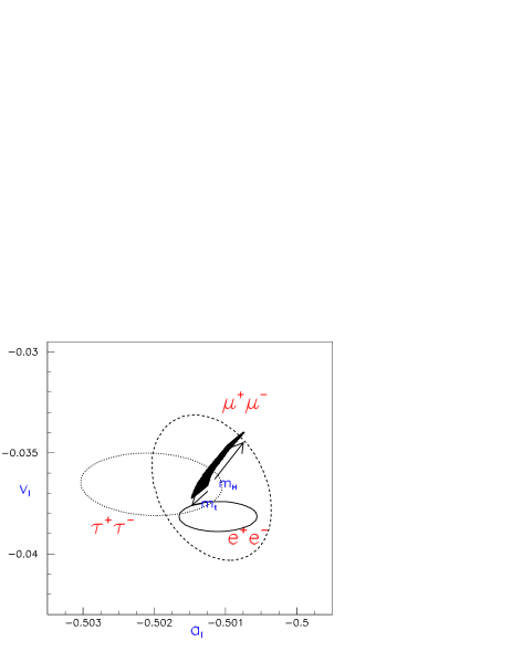
Figure 8: Contours of 70% probability in the $v_{\ell}$-$a_{\ell}$ plane from LEP and SLD measurements. The solid region corresponds to the Standard Model prediction for $169.2\leq m_{\mathrm{t}}~{}[{\rm{GeV}}]\leq 179.4$ GeV and $114\leq m_{\mathrm{H}}~{}[{\rm{GeV}}]\leq 1000$ GeV. The arrows point in the direction of increasing values of $m_{\mathrm{t}}$ and $m_{\mathrm{H}}$.

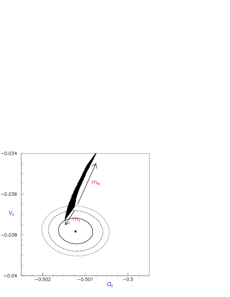
Figure 9: Contours of 70%, 95% and 99% probability in the $v_{\ell}$-$a_{\ell}$ plane from LEP and SLD measurements. The solid region corresponds to the Standard Model prediction for $169.2\leq m_{\mathrm{t}}~{}[{\rm{GeV}}]\leq 179.4$ GeV and $114\leq m_{\mathrm{H}}~{}[{\rm{GeV}}]\leq 1000$ GeV. The arrows point in the direction of increasing values of $m_{\mathrm{t}}$ and $m_{\mathrm{H}}$.

3.8 Heavy Flavour results

It is of intrinsic interest to extract the ${\mathrm{Z}}$ couplings to individual quark flavours, in contrast to the results described in section  3.3, which are summed over 5 flavours. The quantities measured are the ${\mathrm{Z}}$ partial width ratios 

$${R^{0}_{\mathrm{q}}}=\frac{{\Gamma_{\rm q}}}{\Gamma_{\mathrm{had}}}\hskip 28.45274pt({\rm q=b,c}),$$ (36)

the Z-pole forward-backward asymmetries for b and c quarks , $A^{0,\,{\rm b}}_{\rm{FB}}$ and $A^{0,\,{\rm c}}_{\rm{FB}}$, and the direct measurements of $\rm{A_{b}}$ and $\rm{A_{c}}$ by SLD, obtained by measuring $\tilde{\rm{A}}_{FB}^{\rm f}$ (see eqn. 34), for b and c quarks, with a polarised beam. Note that the propagator effects for the t-quark and Higgs, as well as QCD effects, largely cancel in the ratio ${R^{0}_{\mathrm{q}}}$. However, for b-quarks, there are significant SM vertex corrections from tWb couplings. These are essentially independent of $m_{\mathrm{H}}$ and lead to a decrease of ${\Gamma_{{\mathrm{b}\overline{\mathrm{b}}}}}$ with increasing $m_{\mathrm{t}}$, rather than an increase as for the other quark partial-widths. Furthermore, ${R^{0}_{\mathrm{b}}}$ is sensitive to physics beyond the SM (e.g. from light $\tilde{\rm{t}}$,$\tilde{\chi}$ SUSY particles).

Extracting relatively pure samples of events corresponding to individual quark flavours is far from easy. Measurements exist for both c and b quarks, which can be separated from light (u,d,s) quarks, and from each other, using their characteristic properties (see table 8).

Table 8: Some properties of B hadrons and D mesons.

• quantity	B	D+	D0
  lifetime (ps)	1.6	1.0	0.4
  $<$ xE = Ehad/E${}_{beam}>$	0.7	0.5	0.5
  decay charged multiplicity	5.5	2.2	2.2

The main selection criteria (tags) are as follows:-

• c-quarks: D,D^∗ mesons plus lifetime and lepton tags. The harder momentum fraction in direct c decay, compared to b$\rightarrow$c, is also used. For $A_{\mathrm{FB}}^{\mathrm{c}}$, the D/D^∗ charges and the lepton charges, in semileptonic decays, are used to distinguish c from $\bar{c}$.

• b-quarks: lifetime, mass and lepton tags. The mass tag exploits the fact that the b-quark decay products have relatively large invariant masses. For $A_{\mathrm{FB}}^{\mathrm{b}}$, the lepton charge is used, evaluating the contributions from b$\rightarrow\ell$ and b$\rightarrow$c$\rightarrow\ell$, b$\rightarrow\bar{c}\rightarrow\ell$. Also used is the jet-charge for a specific hemisphere with respect to the thrust-axis, Q_hemi= $\sum\mid$p${}^{i}_{\mid\mid}\mid^{\kappa}$ Q_i/ $\sum\mid$p${}^{i}_{\mid\mid}\mid^{\kappa}$, where p${}^{i}_{\mid\mid}$ is the momentum component of a hadron, with charge Q_i, parallel to the thrust axis. The power $\kappa$ is optimised for sensitivity. The charge difference between the forward and backward hemispheres, Q_F-Q_B, is related to the required asymmetry. The sum, Q_F+Q_B, is sensitive to any bias and to the charge resolution. For ${R_{\mathrm{b}}}$, and to a lesser extent for ${R_{\mathrm{c}}}$, the most accurate results are from double-tag methods, as discussed below.

The main background in the tagged b(c) quark sample is from c(b)quarks. This means that the value of ${R^{0}_{\mathrm{b}}}$ is correlated to that of ${R^{0}_{\mathrm{c}}}$. It is usual practice to give ${R^{0}_{\mathrm{b}}}$ at the SM value ${R^{0}_{\mathrm{c}}}$ = 0.172.

The main systematic uncertainties arise from:-

• the fraction of D^∗, D⁺, D_s, $\Lambda_{c}$ etc in ${\rm{c}\bar{\rm{c}}}$ events (particularly important for ${R_{\mathrm{b}}}$)

• b and c hadron lifetimes

• charm decay modes

• fraction of gluon-splitting g $\rightarrow{\rm{c}\bar{\rm{c}}},{\rm{b}\bar{\rm{b}}}$ in hadronic Z events; the values used are the measured fractions g${}_{\rm{c}\bar{\rm{c}}}$ = (2.96 $\pm$ 0.38)% and g${}_{\rm{b}\bar{\rm{b}}}$ = (0.25 $\pm$ 0.05)%

• semi-leptonic branching ratios and decay models

• light quark fragmentation models

• correlations between hemispheres for double-tags.

3.9 Measurement of ${R_{\mathrm{b}}}$

The most accurate measurements of ${R_{\mathrm{b}}}$ all employ a double-tag method. This involves determining the jet axis of the event (thrust-axis) and then employing lifetime, mass, leptonic or other b-tags to each hemisphere to determine the number of hemispheres N_t, with a tag, and the number of events N_tt, with two tags. For a sample of N_had hadronic ${\mathrm{Z}}$ decays one has

$$\frac{N_{t}}{2N_{\rm{had}}}=\epsilon_{b}R_{\mathrm{b}}+\epsilon_{c}R_{\mathrm{c}}+\epsilon_{uds}(1-R_{\mathrm{b}}-R_{\mathrm{c}}),\\$$ (37)

$$\frac{N_{tt}}{N_{\rm{had}}}={{\cal C}_{\rm b}}{(\epsilon_{b})^{2}R_{\mathrm{b}}}+(\epsilon_{c})^{2}R_{\mathrm{c}}+(\epsilon_{uds})^{2}(1-R_{\mathrm{b}}-R_{\mathrm{c}}),$$ (38)

where $\epsilon_{b}$, $\epsilon_{c}$ and $\epsilon_{uds}$ are the tagging efficiencies per hemisphere for b, c and light-quark events, and ${\cal C}_{\rm b}\neq 1$ accounts for the fact that the tagging efficiencies between the hemispheres may be correlated. In practice, $\epsilon_{b}\gg\epsilon_{c}\gg\epsilon_{uds}$, ${\cal C}_{\rm b}\approx 1$, and the correlations for the other flavours are neglected. These equations can be solved to give $R_{\mathrm{b}}$ and $\epsilon_{b}$ which, neglecting the c and uds backgrounds and the correlations, are approximately given by:

$$\epsilon_{b}\approx 2N_{tt}/N_{t},\\$$ (39)

$$R_{\mathrm{b}}\approx N_{t}^{2}/(4N_{tt}N_{\rm{had}}).$$ (40)

The double-tagging method has the advantage that the tagging efficiency is determined directly from the data, reducing the systematic error of the measurement. The residual background of other flavours in the sample, and the evaluation of the correlation between the tagging efficiencies in the two hemispheres of the event, are the main sources of systematic uncertainty in such an analysis. The use of powerful vertex detectors at LEP has led to excellent b-tagging efficiencies. For example, DELPHI achieves 30%, with a 1.5% background. Due, at least in part, to the closer proximity to the interaction point an even better performance (50% with a 2% background) is achieved by SLD. The single/double-tag method has been extended by ALEPH and DELPHI to multi-tags. This not only improves the statistical accuracy, but also reduces the systematic uncertainty due to hemisphere correlations and charm contamination.

The results for $R_{\mathrm{b}}$ are shown in fig. 10. The combined LEP/SLD value of ${R^{0}_{\mathrm{b}}}=$ 0.21646 $\pm$ 0.00065 thus has a relative precision of about 0.3%. The average value, when interpreted in terms of the SM, gives a value of $m_{\mathrm{t}}$ = 155 ${}^{+19+1}_{-21-0}$ GeV, where the central value is for $m_{\mathrm{H}}$ = 150 GeV and the second error corresponds to the range $114\leq m_{\mathrm{H}}~{}[{\rm{GeV}}]\leq 1000$, and the constraint $\alpha_{\rm{s}}{\rm(m_{\mathrm{Z}})}$ = 0.118 $\pm$ 0.002 is used. This is consistent with the direct determination [39]. The combined statistical error of all the $R_{\mathrm{b}}$ measurements is 0.00043 and that from the internal experimental systematics (track resolution, detection efficiencies of leptons etc) is 0.00029. The error due to common systematics is about 0.00039. The largest common systematic errors are from uncertainties on gluon splitting into b and c quark pairs (0.00022), QCD effects in hemisphere correlations (0.00018) and the branching ratio D $\rightarrow$ neutrals (0.00014). In total, more than 20 possible sources of systematic error to ${R_{\mathrm{b}}}$ are considered.

At the time of the Summer Conferences in 1995, the average value was ${R^{0}_{\mathrm{b}}}$ = 0.2205 $\pm$ 0.0016 (for ${R^{0}_{\mathrm{c}}}$ = 0.172) [40], more than three standard deviations above the SM value. The measured value was in the direction expected from light SUSY particles  ($\tilde{\rm{t}}$,$\tilde{\chi}$). However, SUSY particles in the mass range suggested by the excess in ${R^{0}_{\mathrm{b}}}$ have since been excluded by searches at LEP 2. The subsequent change in the ${R^{0}_{\mathrm{b}}}$ average is due to a combination of much improved statistics, purer tagging methods and changes of some of the heavy flavour input parameters needed in the analysis.

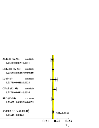
Figure 10: Results on ${R_{\mathrm{b}}}$, for ${R_{\mathrm{c}}}$ = 0.172, together with the average value for ${R^{0}_{\mathrm{b}}}$, from a fit to all the LEP and SLC heavy flavour data. The SM prediction for $m_{\mathrm{t}}$ = 174.3 GeV and $m_{\mathrm{H}}$ = 150 GeV is shown as a dashed line.

3.10 Measurement of ${R_{\mathrm{c}}}$

Tagging charm quarks with high efficiency and purity is unfortunately difficult. The cleanest tag is to use the decay sequence c$\rightarrow{\rm D}^{*+}\rightarrow{\rm D}^{0}\pi^{+}({\rm D}^{0}\rightarrow$K${}^{-}\pi^{+}$), but this tags only about 0.5% of c-decays, so is statistically limited. Other ${\rm D}^{0}$ modes, which are somewhat less clean, can also be used, as can other ground-state charmed hadrons and c-quark leptonic decays. The purities achieved are 65-90%, but with an overall charm tag efficiency of only a few percent.

There are also analyses which use a ‘slow’ $\pi$ tag (the $\pi$ in the D^∗ decay has a small p_T) in a double-tag. However, this tag is rather loose because there is a considerable background at low p_T from fragmentation processes.

Several methods have been used in the determination of $R_{\mathrm{c}}$. These are:

• Single charm-counting rate (ALEPH, DELPHI and OPAL). This requires measuring the production rates of the ground-state charmed hadrons (${\rm D}^{0},{\rm D}^{+},{\rm{D_{s}}}$, as well as charmed baryons). Small corrections are applied for unobserved baryonic states. The total rate gives $R_{\mathrm{c}}$ x Prob(c$\rightarrow$ hadrons), so if all the ground-state charmed hadrons are detected the measurement gives $R_{\mathrm{c}}$.

• Inclusive/exclusive double-tag (ALEPH, DELPHI and OPAL). This first requires measurements of the production rate of ${\mathrm{D}}^{*\pm}$ mesons in several decay channels. This depends on the product $R_{\mathrm{c}}$ x P${}_{c\rightarrow{\rm D}^{*+}}$ x BR(${\rm D}^{*+}\rightarrow{\rm D}^{0}\pi^{+}$), and this sample of ${\rm{c}\bar{\rm{c}}}$ (and ${\rm{b}\bar{\rm{b}}}$) events is used to measure P${}_{c\rightarrow{\rm D}^{*+}}$ x BR(${\rm D}^{*+}\rightarrow{\rm D}^{0}\pi^{+}$), using a slow pion tag in the opposite hemisphere.

• Exclusive double-tag (ALEPH). Here, exclusively reconstructed ${\rm D}^{*+}$, ${\rm D}^{+}$ and ${\rm D}^{0}$ mesons are used, giving good purity but larger statistical errors.

• Lifetime plus mass double-tag (SLD). This uses the same tagging algorithm used for $R_{\mathrm{b}}$, and achieves a purity of about 84%.

• Single leptons (ALEPH). This assumes a value of BR(c$\rightarrow$l).

The LEP average value for ${R^{0}_{\mathrm{c}}}$, made in Summer 1995, was ${R^{0}_{\mathrm{c}}}$ = 0.1540 $\pm$ 0.0074. This was some 2.4 standard deviations below the SM value of 0.172. The present value (see fig. 11) is ${R^{0}_{\mathrm{c}}}$ = 0.1719 $\pm$ 0.0031, and is rather close to the SM value. For the 1995 average, roughly half of the error weight came from common systematic errors between the measurements, which relied in particular on the measurement of Y_c = P(c$\rightarrow{\rm D}^{*+}$) x BR(${\rm D}^{*+}\rightarrow\pi^{+}$) made at low ($\sqrt{s}\sim$ 10 GeV) energy. The LEP data now determine this quantity directly, so that the present average does not depend on the use of low energy data. In addition techniques have been refined and more robust analyses performed.

The relative precision of the average value of ${R^{0}_{\mathrm{c}}}$ is 1.8%. The statistical component of the error is 0.0023, and that from internal experimental systematics 0.0014. The total common systematic error is 0.0014, with the largest components (0.0005) coming from both BR(${\rm{D_{s}}}\rightarrow\phi\pi$) and BR($\Lambda_{c}\rightarrow$pK${}^{-}\pi^{+}$).

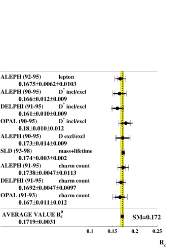
Figure 11: Results on ${R_{\mathrm{c}}}$, together with the average value for ${R^{0}_{\mathrm{c}}}$, from a fit to all the LEP and SLC heavy flavour data. The SM prediction for $m_{\mathrm{t}}$ = 174.3 GeV and $m_{\mathrm{H}}$ = 150 GeV is shown as a dashed line.

As discussed above, the determinations of ${R^{0}_{\mathrm{b}}}$ and ${R^{0}_{\mathrm{c}}}$ are correlated, with a correlation coefficient of -0.14. Fig. 12 shows the 70% and 95% confidence level contours in the ${R^{0}_{\mathrm{b}}}$, ${R^{0}_{\mathrm{c}}}$ plane, as well as the SM prediction for various values of $m_{\mathrm{t}}$.

Figure 12: The 70% and 95% confidence level contours in the ${R^{0}_{\mathrm{b}}}$, ${R^{0}_{\mathrm{c}}}$ plane. The SM prediction for various values of $m_{\mathrm{t}}$ is shown, as is the central experimental value in 1995, together with its 95% confidence level contour.

3.11 Heavy-quark asymmetries

The results for $A_{\mathrm{FB}}^{\mathrm{b}}$ and $A_{\mathrm{FB}}^{\mathrm{c}}$ are given in figs. 13 and  14 respectively. They are corrected to the full experimental acceptance. The quoted values are corrected for QCD effects and to correspond to $\sqrt{s}=$ 91.26 GeV; both peak and off-peak data are used. The QCD corrections are calculated to second-order [41], and amount to 0.0063 for both b and c quarks [42]. In order to obtain the pole asymmetries $A^{0,\,{\rm c}}_{\rm{FB}}$ and $A^{0,\,{\rm b}}_{\rm{FB}}$ from the experimentally measured results, corrections are applied, using ZFITTER, to get to $\sqrt{s}=m_{\mathrm{Z}}$, for QED effects and for the contributions of $\gamma$ exchange and $\gamma-\mbox{${\mathrm{Z}}$}$ interference, as well as for the b-quark mass. These amount, in total, to additive corrections of 0.0062 for $A_{\mathrm{FB}}^{\mathrm{c}}$ and 0.0025 for $A_{\mathrm{FB}}^{\mathrm{b}}$. The results for $A_{\mathrm{FB}}^{\mathrm{b}}$ have also been corrected for the effects of ${\rm{b}\bar{\rm{b}}}$ mixing. The methods used for the asymmetries are as follows:

• Lepton spectra (ALEPH, DELPHI, L3 and OPAL). The characteristic high transverse momentum spectrum from the heavy quarks is exploited (sometimes in conjunction with other information) to measure both $A_{\mathrm{FB}}^{\mathrm{b}}$ and $A_{\mathrm{FB}}^{\mathrm{c}}$.

• Lifetime tag plus hemisphere charge (ALEPH, DELPHI, L3 and OPAL). For $A_{\mathrm{FB}}^{\mathrm{b}}$, and these give roughly equal precision to the lepton results.

• D mesons (ALEPH for $A_{\mathrm{FB}}^{\mathrm{c}}$, and DELPHI and OPAL for $A_{\mathrm{FB}}^{\mathrm{b}}$ and $A_{\mathrm{FB}}^{\mathrm{c}}$).

Neural Network methods have also been used for the most recent measurements of $A_{\mathrm{FB}}^{\mathrm{b}}$ (ALEPH and DELPHI), incorporating much of the information from the above methods. A single and double-tag procedure is used, as for ${R_{\mathrm{b}}}$, so the method is essentially self-calibrating, except for the effects of backgrounds and hemisphere correlations, which are taken from simulation.

For both the $A_{\mathrm{FB}}^{\mathrm{b}}$ and $A_{\mathrm{FB}}^{\mathrm{c}}$ measurements, the systematic errors in all the methods are smaller than the statistical errors. For $A_{\mathrm{FB}}^{\mathrm{b}}$ the statistical, internal systematic and common systematic components of the errors are 0.0016, 0.0006 and 0.0004 respectively. For $A_{\mathrm{FB}}^{\mathrm{c}}$ the statistical, internal systematic and common systematic components of the errors are 0.0030, 0.0014 and 0.0009 respectively. So both these measurements are statistics limited.

The asymmetries $A^{0,\,{\rm b}}_{\rm{FB}}$ and $A^{0,\,{\rm c}}_{\rm{FB}}$ are rather weakly correlated, and both the pole asymmetries, and their energy dependence (see fig. 15), are compatible with the SM.

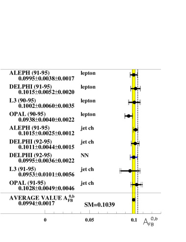
Figure 13: Results on $A_{\mathrm{FB}}^{\mathrm{b}}$, together with the average value for $A^{0,\,{\rm b}}_{\rm{FB}}$ from a fit to all the LEP heavy flavour data. The SM prediction for $m_{\mathrm{t}}$ = 174.3 GeV, $m_{\mathrm{H}}$ = 150 GeV is shown as a dashed line.

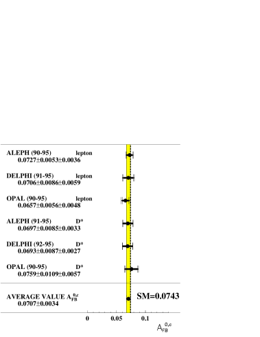
Figure 14: Results on $A_{\mathrm{FB}}^{\mathrm{c}}$, together with the average value for $A^{0,\,{\rm c}}_{\rm{FB}}$ from a fit to all the LEP heavy flavour data. The lepton results shown are still preliminary. An earlier lepton result from L3 is included in the average but not plotted. The SM prediction for $m_{\mathrm{t}}$ = 174.3 GeV, $m_{\mathrm{H}}$ = 150 GeV is shown as a dashed line.

Measurements of the heavy-quark forward-backward asymmetries, using a longitudinally polarised beam, by the SLD Collaboration give directly values of $\rm{A_{b}}$ and $\rm{A_{c}}$. Using lepton, kaon, D-meson and jet-charge plus lifetime/vertex mass tags, the values $\rm{A_{b}}$ = 0.922 $\pm$ 0.020 and $\rm{A_{c}}$ = 0.670 $\pm$ 0.026 are obtained [43, 8].

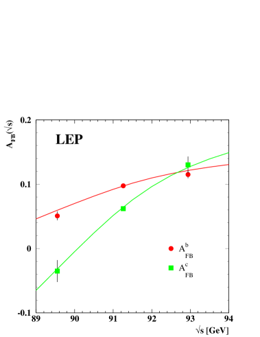
Figure 15: Energy dependence of the heavy-quark forward-backward asymmetries.

3.12 Combining the heavy flavour results

The combination has been carried out by a LEP/SLD working group [8], and details of the procedure used for the LEP experiments can be found in  [44]. Each experiment provides, for each measurement, a complete breakdown of the systematic errors, adjusted if necessary to agreed meanings of these errors. Direct measurements of $\rm{A_{b}}$ and $\rm{A_{c}}$ by SLD, obtained by measuring $A_{\mathrm{FB}}^{\mathrm{b}}$ and $A_{\mathrm{FB}}^{\mathrm{c}}$ with a polarised beam, are also included. A multi-parameter fit is then performed to get the best overall values of ${R^{0}_{\mathrm{b}}}$,${R^{0}_{\mathrm{c}}}$,$A^{0,\,{\rm b}}_{\rm{FB}}$, $A^{0,\,{\rm c}}_{\rm{FB}}$, $\rm{A_{b}}$ and $\rm{A_{c}}$, plus their covariance matrix. The results of a fit to both the LEP and SLD data are given in table 9. The effective mixing parameter $\bar{\chi}$, and the leptonic branching ratios b$\rightarrow\ell$, b$\rightarrow$c$\rightarrow\bar{\ell}$ and c$\rightarrow\ell$, are also included in the fit. It should be noted that the $\chi^{2}$/df is very small, leading to a probability close to 100$\%$. This is, of course, rather unlikely. However, it does indicate that the errors on the combined heavy flavour results are probably not underestimated.

Table 9: Results of fits to the LEP and SLD heavy flavour data, plus the correlation matrix. The $\chi^{2}$/df of the average is 47/(105-14), a probability of greater than 99$\%$.

• quantity	value	error	${R^{0}_{\mathrm{b}}}$	${R^{0}_{\mathrm{c}}}$	$A^{0,\,{\rm b}}_{\rm{FB}}$	$A^{0,\,{\rm c}}_{\rm{FB}}$	$\cal A_{\rm b}$	$\cal A_{\rm c}$
  ${R^{0}_{\mathrm{b}}}$	0.21646	0.00065	1.000	–0.14	–0.08	0.05	–0.07	0.04
  ${R^{0}_{\mathrm{c}}}$	0.1719	0.0031		1.000	0.04	–0.03	0.03	–0.05
  $A^{0,\,{\rm b}}_{\rm{FB}}$	0.0994	0.0017			1.000	0.16	0.02	0.00
  $A^{0,\,{\rm c}}_{\rm{FB}}$	0.0707	0.0034				1.000	–0.01	0.02
  $\cal A_{\rm b}$	0.922	0.020					1.000	0.13
  $\cal A_{\rm c}$	0.670	0.026						1.000

3.13 Inclusive Hadron Charge Asymmetry ${\langle\mbox{\rm Q}_{\mbox{\rm FB}}\rangle}$

Asymmetry measurements can also be made if the individual quark flavours are not separated. The method involves the measurement, in ${\mathrm{Z}}$ hadronic events, of the hadronic charge asymmetry, based on the mean difference in jet charges measured in the forward and backward event hemispheres, ${\langle\mbox{\rm Q}_{\mbox{\rm FB}}\rangle}$. The measured values of ${\langle\mbox{\rm Q}_{\mbox{\rm FB}}\rangle}$ cannot be compared directly as some of them include detector dependent effects, such as acceptances and efficiencies. The results are best compared using the values of $\sin^{2}\!\theta_{\rm{eff}}^{\rm{lept}}$ extracted in each analysis, as given in table 10. It can be seen that the systematic errors are larger than the statistical errors. These are dominated by fragmentation and decay modelling uncertainties.

Table 10: Summary of the determinations of $\sin^{2}\!\theta_{\rm{eff}}^{\rm{lept}}$ from inclusive hadronic charge asymmetries at LEP. For each experiment, the first error is statistical and the second systematic.

• Experiment		$\sin^{2}\!\theta_{\rm{eff}}^{\rm{lept}}$
  ALEPH	90-94	$0.2322\pm 0.0008\pm 0.0011$
  DELPHI	91	$0.2345\pm 0.0030\pm 0.0027$
  L3	91-95	$0.2327\pm 0.0012\pm 0.0013$
  OPAL	90-91	$0.2326\pm 0.0012\pm 0.0029$
  Average		$0.2324\pm 0.0012$

3.14 The coupling parameters $\cal A_{\rm f}$

The coupling parameters $\cal A_{\rm f}$ are obtained directly in the case of the SLD polarisation measurements or from the $\tau$ lepton polarisation. The forward-backward asymmetries for different fermions at LEP, using eqn.(25), determine the product of $\cal A_{\rm e}$ and $\cal A_{\rm f}$. The results for $\cal A_{\rm e}$, determined assuming lepton universality where appropriate, are given in table 11. The results for $\cal A_{\rm b}$ and $\cal A_{\rm c}$, both those measured directly and those derived from forward-backward asymmetry measurements and assuming a value of $\cal A_{\rm e}$, are given in table 12. The results are displayed graphically in fig 16.

Table 11: Determinations of the leptonic coupling parameter $\cal A_{\ell}$, assuming lepton universality. The cumulative averages for $\cal A_{\ell}$, and the $\chi^{2}$ per degree of freedom for these, are also given.

• 	$\cal A_{\ell}$	Cumulative Average	$\chi^{2}$/df
  $A^{0,\,\ell}_{\rm{FB}}$	$0.1512\pm 0.0042$
  $\mbox{$\cal P_{\tau}$}(\cos\theta)$	$0.1465\pm 0.0033$	$0.1482\pm 0.0026$	0.8/1
  $\cal A_{\ell}$ (SLD)	$0.1513\pm 0.0021$	$0.1501\pm 0.0016$	1.6/2

Table 12: Determination of the quark coupling parameters $\cal A_{\rm b}$ and $\cal A_{\rm c}$ from LEP data alone (using the LEP average for $\cal A_{\ell}$), from SLD data alone, and from LEP+SLD data (using the LEP+SLD average for $\cal A_{\ell}$), assuming lepton universality.

• 	LEP	SLD	LEP+SLD
  	($\mbox{$\cal A_{\ell}$}=0.1482\pm 0.0026$)		($\mbox{$\cal A_{\ell}$}=0.1501\pm 0.0016$)
  $\cal A_{\rm b}$	$0.893\pm 0.022$	$0.922\pm 0.020$	$0.901\pm 0.013$
  $\cal A_{\rm c}$	$0.634\pm 0.033$	$0.670\pm 0.026$	$0.653\pm 0.020$

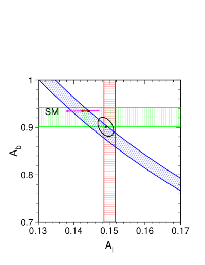
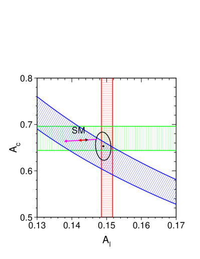
Figure 16: Measurements of $\cal A_{\ell}$ from SLD+LEP (vertical band), $\cal A_{\rm b}$($\cal A_{\rm c}$) from SLD (horizontal band) and $A^{0,\,{\rm b}}_{\rm{FB}}$($A^{0,\,{\rm c}}_{\rm{FB}}$) from LEP (diagonal band). The 70$\%$ confidence level contour for the combined fit to these variables is also shown. The SM predictions are shown as arrows, with the left-pointing arrow showing the variation from $m_{\mathrm{H}}$ = 300${}^{+700}_{-186}$ GeV and the right-pointing arrow showing the variation from $m_{\mathrm{t}}$ = 174.3 $\pm$ 5.1 GeV. There is an additional contribution from the error on $\Delta\alpha^{(5)}_{\rm had}$ ($\pm$ 0.00036), which is in the same sense as the Higgs arrow but with a size similar to that from the top-quark uncertainty.

Figure 17: Results of a fit to the b and c quark vector and axial-vector couplings. The contours are for the 70, 95 and 99% confidence limits. The SM predictions are also shown.

It can be seen that the SLD values of $\cal A_{\rm b}$ and $\cal A_{\rm c}$ are in good agreement with the SM predictions of 0.935 and 0.668, which are essentially independent of $m_{\mathrm{t}}$ and $m_{\mathrm{H}}$. However, the values of $\cal A_{\rm b}$ and $\cal A_{\rm c}$, extracted from $A^{0,\,{\rm b}}_{\rm{FB}}$ and $A^{0,\,{\rm c}}_{\rm{FB}}$ and the measured values of $\cal A_{\rm e}$, are somewhat below the SM predictions. When combined with the SLD results, which for $\cal A_{\rm b}$ is slightly below the SM prediction, the values for $\cal A_{\rm b}$ and $\cal A_{\rm c}$ are respectively 2.6 and 0.8 standard deviations below the SM predictions.

3.15 Extraction of heavy-quark couplings

An alternative approach in trying to understand the possible implications of the heavy flavour results is to extract the individual quark couplings[45]. The measurements used are ${R^{0}_{\mathrm{b}}}={\Gamma_{{\mathrm{b}\overline{\mathrm{b}}}}}/\Gamma_{\mathrm{had}}$ (which, using $\Gamma_{\mathrm{had}}$ from the lineshape, gives $v_{\rm{b}}^{2}$+ $a_{\rm{b}}^{2}$), ${R^{0}_{\mathrm{c}}}$ ($v_{\rm{c}}^{2}$ + $a_{\rm{c}}^{2}$), $\cal A_{\rm e}$ from LEP/SLD ($v_{\rm{e}}/a_{\rm{e}}$), $A^{0,\,{\rm b}}_{\rm{FB}}$ ($v_{\rm{b}}/a_{\rm{b}}$, $v_{\rm{e}}/a_{\rm{e}}$), $\rm{A_{b}}$ ($v_{\rm{b}}/a_{\rm{b}}$), $A^{0,\,{\rm c}}_{\rm{FB}}$ ($v_{\rm{c}}/a_{\rm{c}}$, $v_{\rm{e}}/a_{\rm{e}}$) and $\rm{A_{c}}$ ($v_{\rm{c}}/a_{\rm{c}}$). The constraint $\alpha_{\rm{s}}{\rm(m_{\mathrm{Z}})}$ = 0.118 $\pm$ 0.002 is imposed (although the results are rather insensitive to this, as discussed below), and lepton universality is assumed.

The signs of the b- and c-quark couplings are uniquely determined from the LEP data. From the sign of the measured value of $A^{0,\,{\rm b}}_{\rm{FB}}$ (i.e. positive), it follows that $v_{\rm{b}}$ and $a_{\rm{b}}$ have the same sign. The behaviour of the energy dependence of A${}_{FB}^{b}$ away from the Z-pole depends on the product Q_eQ${}_{\rm b}a_{\rm{e}}a_{\rm{b}}$ of the electric charges and axial-vector couplings of the electron and b-quark. From the data shown in fig. 15 it can thus be deduced that $a_{\rm{b}}$ is negative, and thus $v_{\rm{b}}$ is also negative. Similar considerations show that $v_{\rm{c}}$ and $a_{\rm{c}}$ are both positive. The results for the vector and axial-vector couplings, of both b and c quarks, are shown in table  13 and fig. 17. Also shown are the SM predictions corresponding to $m_{\mathrm{t}}=174.3\pm 5.1$ GeV and $114\leq m_{\mathrm{H}}~{}[{\rm{GeV}}]\leq 1000$. Note that there is a very strong anti-correlation between $v_{\rm{b}}$ and $a_{\rm{b}}$. As discussed above, the signs and magnitudes of all the couplings have been determined. These confirm the SM quantum number assignments. Of course, they are measured to good precision, so the results are sensitive to small deviations from the simplest predictions.

Table 13: Results, plus correlation matrix, of a fit to the vector and axial-vector couplings of b and c quarks. The $\chi^{2}$ probability for the fit is 11%.

• parameter	fitted value	$v_{\rm{b}}$	$a_{\rm{b}}$	$v_{\rm{c}}$	$a_{\rm{c}}$
  $v_{\rm{b}}$	$-0.3233\pm 0.0079$	1.00	-0.97	-0.19	0.06
  $a_{\rm{b}}$	$-0.5139\pm 0.0052$		1.00	0.18	-0.03
  $v_{\rm{c}}$	$0.1873\pm 0.0068$			1.00	-0.29
  $a_{\rm{c}}$	$0.5032\pm 0.0053$				1.00

The b-quark couplings can also be expressed in terms of the left-handed $\ell_{b}$ = ($v_{\rm{b}}$ + $a_{\rm{b}}$)/2 and right-handed r_b = ($v_{\rm{b}}$ - $a_{\rm{b}}$)/2 couplings. The results are shown in fig. 18. The corresponding results for the c-quark are also shown. The b-quark couplings are not in particularly good agreement with the SM predictions, with the largest discrepancy being for the right-handed coupling, r_b.

The fitted values of $v_{\rm{b}}$ and $a_{\rm{b}}$ (or $\ell_{b}$ and r_b) give a value of ${R^{0}_{\mathrm{b}}}$ greater than the SM value, and a value of $\cal A_{\rm b}$ (or $A^{0,\,{\rm b}}_{\rm{FB}}$) less than the SM value. In that sense the b-quark data are mutually consistent with the observed deviations from the  SM. The point in the SM band giving the smallest $\chi^{2}$ to the fitted data values corresponds to $m_{\mathrm{t}}$ = 169.2 GeV and $m_{\mathrm{H}}$ = 114 GeV. The $\chi^{2}$ probability for compatibility to this point is 2.8%.

It is worthwhile therefore exploring further this possible discrepancy. In the above fits the assumed value of $\alpha_{\rm{s}}{\rm(m_{\mathrm{Z}})}$ was taken to be 0.118 $\pm$ 0.002. If a central value of 0.116 is used, then the leptonic couplings are unchanged and the shifts in the b- and c-quark couplings are less than 0.0002. Hence the results are not very sensitive to $\alpha_{\rm{s}}{\rm(m_{\mathrm{Z}})}$. This is to be expected since the ratios ${R^{0}_{\mathrm{b}}}$ and ${R^{0}_{\mathrm{c}}}$ are, by construction, rather insensitive to $\alpha_{\rm{s}}{\rm(m_{\mathrm{Z}})}$.

The results from the SLD Collaboration on $A_{\rm{LR}}$, $\rm{A_{b}}$ and $\rm{A_{c}}$ [43, 8] require a precise determination of the degree of polarisation of the electron beam. It can be noted that the values of $\cal A_{\rm e}$ (from $A_{\rm{LR}}$), $\rm{A_{b}}$ (from $\tilde{\rm{A}}_{FB}^{\rm b}$, see eqn.34) are above and below the SM predictions respectively. Since, in both cases, what is measured is proportional to the product of the polarisation and the required parameter, the measurements cannot both be reconciled with the SM simply by a change in the value of the electron polarisation. It is worth stressing that the uncertainty on $A_{\rm{LR}}$ due to the polarisation is about 0.5%. This is to be compared to the overall statistical component of the error of about 1.3%.

Measurements of $A^{0,\,{\rm b}}_{\rm{FB}}$ determine the product of $\cal A_{\rm e}$ and $\rm{A_{b}}$. Thus the value of $\rm{A_{b}}$ extracted depends critically on that of $\cal A_{\rm e}$. In the standard fits given above the information on $\cal A_{\rm e}$ comes from all of the data, and the fitted value is $\cal A_{\rm e}$  = 0.1501 $\pm$ 0.0016. Most of the information comes from the measurements of $A_{\rm{LR}}$, the $\tau$-polarisation and $A^{0,\,\ell}_{\rm{FB}}$. In the SM the value of $\cal A_{\rm e}$ increases for increasing $m_{\mathrm{t}}$ and decreasing $m_{\mathrm{H}}$. However, as $m_{\mathrm{t}}$ is now well constrained, the main variation is from $m_{\mathrm{H}}$. As can be seen from fig. 8, the lepton coupling data favour a light Higgs. Within the ranges $169.2\leq m_{\mathrm{t}}~{}[{\rm{GeV}}]\leq 179.4$ and $114\leq m_{\mathrm{H}}~{}[{\rm{GeV}}]\leq 1000$, the closest SM value is 0.1485, which corresponds to $m_{\mathrm{t}}$ = 179.4 GeV and $m_{\mathrm{H}}$ = 114 GeV. The values of $v_{\rm{b}}$ and $a_{\rm{b}}$ extracted, when this value for $\cal A_{\rm e}$ is imposed for the measurement of $A^{0,\,{\rm b}}_{\rm{FB}}$, are given in table 14. Also given are the $\chi^{2}$ probabilities that the results are compatible with this SM point. If $A^{0,\,{\rm b}}_{\rm{FB}}$ and $A^{0,\,{\rm c}}_{\rm{FB}}$ are removed from the fit, then the probability increases to 38%.

In summary, the fit to the couplings gives a satisfactory $\chi^{2}$, and the fitted vector and axial-vector couplings are reasonably compatible with the SM values. The largest contribution to the fit $\chi^{2}$ comes from the measurement of $A^{0,\,{\rm b}}_{\rm{FB}}$.

Figure 18: Results of a fit to the b and c quark left-handed and right-handed couplings. The contours are for the 70, 95 and 99% confidence limits.

Table 14: Values of $v_{\rm{b}}$ and $a_{\rm{b}}$ for different assumptions about the use of $A^{0,\,{\rm b}}_{\rm{FB}}$. The SM values used correspond to $m_{\mathrm{H}}$ = 114 GeV and $m_{\mathrm{t}}$ = 169.2 GeV, except for the second line where $m_{\mathrm{t}}$ = 179.4 GeV is used for consistency with the value of $\cal A_{\rm e}$.

• conditions on $A^{0,\,{\rm b}}_{\rm{FB}}$	$v_{\rm{b}}$	$a_{\rm{b}}$	$\chi^{2}$ prob. for SM
  none	-0.3233 $\pm$ 0.0079	-0.5139 $\pm$ 0.0052	2.8%
  $\cal A_{\rm e}$ = 0.1485	-0.3246 $\pm$ 0.0072	-0.5130 $\pm$ 0.0048	2.3%
  remove $A^{0,\,{\rm b}}_{\rm{FB}}$($A^{0,\,{\rm c}}_{\rm{FB}}$)	-0.3356 $\pm$ 0.0128	-0.5058 $\pm$ 0.0088	38%

3.16 ${\mathbf{f\overline{f}}}$ production at LEP 2

The above results have all come from data collected at energies at, or close to, the ${\mathrm{Z}}$ peak (LEP 1 phase). Data have also been collected at various centre-of-mass energies from 130 to 209 GeV, from 1995 until 2000, when LEP was closed. The part of the programme with centre-of-mass energies above the W-boson pair-production threshold (161 GeV) is called the LEP 2 phase. In total, an integrated luminosity of more than 700 pb^-1 per experiment was collected; well beyond the initially expected luminosity of 500 pb^-1 per experiment.

The reaction $\mathrm{e}^{+}\mathrm{e}^{-}\rightarrow{\rm f}\overline{\rm f}$ has also been extensively studied at LEP 2 energies. For energies well above $\sqrt{s}\simeq m_{\mathrm{Z}}$, the contribution from the Z propagator (see equation 20) is much reduced, as the distance in $\sqrt{s}$ from the Z-pole is many factors of the Z width. However, the main difference in the analysis of LEP 2 ${\rm f}\overline{\rm f}$ data is that there is a significant probablility that an initial state photon (see fig. 3), or photons, are emitted, leaving the energy of the remaining $\mathrm{e}^{+}\mathrm{e}^{-}$ system ($\sqrt{s^{\prime}}$) close to that of the Z resonance. Since the Z cross-section is large, there is a relatively large probability for the process of radiative return to the Z. To study the physics of the direct (or non-radiative) process, it is generally required to have $\sqrt{s^{\prime}}/\sqrt{s}>$ 0.85.

The cross-sections and forward-backward asymmetries for the combined LEP 2 data [8], are shown in fig. 19, together with the Standard Model predictions. It can be seen that the data are in reasonably good agreement with these predictions. This shows that the use of the SM in the calculation of some of the small corrections used in the Z lineshape analyses is well justified. In particular, the $\gamma$-Z interference term for the $q\bar{q}$ final states is poorly known from the Z-pole data, and is fixed to the SM value (see sect. 3.4). This interference term is highly correlated with the ${\mathrm{Z}}$ mass parameter and, if left free in the fit, leads to a much reduced precision on $m_{\mathrm{Z}}$. The data from LEP 2, and also from the TRISTAN accelerator operating at around $\sqrt{s}\simeq$ 61 GeV, can be used to significantly limit the size of the hadronic $\gamma$-Z interference. Although detailed fits have not yet been performed, the error on $m_{\mathrm{Z}}$ with this interference term free should be about 2.3 MeV, compared to that of 2.1 MeV obtained when the SM constraint is imposed. Heavy flavour production rates and asymmetries have also been studied at LEP 2. Again the results are compatible with the SM.

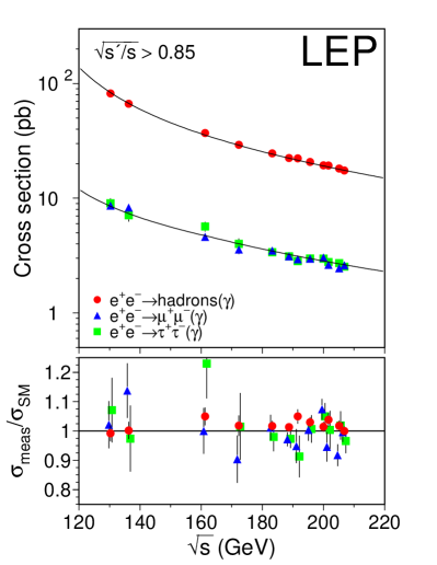
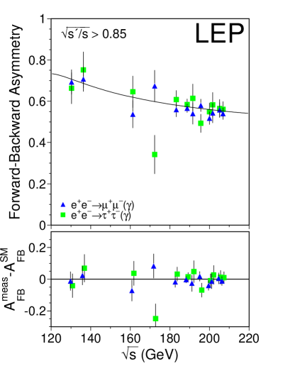
Figure 19: Combined preliminary LEP cross-sections for $q\bar{q}$, $\mu^{+}\mu^{-}$ and $\tau^{+}\tau^{-}$ final states, and forward-backward asymmetries for $\mu^{+}\mu^{-}$ and $\tau^{+}\tau^{-}$ final states, as a function of centre-of-mass energy. The predictions of the Standard Model, computed with ZFITTER, are shown as curves. The lower plots show the ratio of the data divided by the predictions for the cross-sections, and the difference between the measurements and the predictions for the asymmetries.

The ${\rm f}\overline{\rm f}$ data can also set very stringent limits on many models containing physics beyond the Standard Model. These models include additional heavy Z vector bosons, lepto-quarks, R-parity violating supersymmetry, models of gravity in extra dimensions as well as contact interaction models which parameterise new physics in terms of the left- and right-handed components of the initial and final-state fermions. There is no evidence in the data for the existence of any of these effects, and so limits are obtained on the masses or scales below which such effects can be ruled out. For example, the limit on a hypothetical heavy Z-boson, having the same couplings as the ${\mathrm{Z}}$ (sequential Z-boson), can be ruled out for masses up to 1.9 TeV.

In the absence of new physics beyond the SM the $\mathrm{f}\bar{\mathrm{f}}$ data on cross-sections and asymmetries can be used the test the running of the electromagnetic coupling constant $\alpha$. The OPAL Collaboration find a value 1/$\alpha$(191 GeV) = 126.2 $\pm$ 2.2 [46], in agreement with the SM expectation of 127.9.

3.17 The Drell-Yan process

A process analogous to the $\mathrm{e}^{+}\mathrm{e}^{-}\rightarrow{\rm f}\overline{\rm f}$ interaction which has been studied at LEP is $q\bar{q}\rightarrow\ell^{+}\ell^{-}$, the Drell-Yan process [47]. This is studied at the $p\bar{p}$ Tevatron Collider, at Fermilab in the USA, for both electrons and muons in the final state. The interest for electroweak physics is in the region where the $\ell^{+}\ell^{-}$ pair has a large invariant mass. Measurements [48] of the invariant mass distributions, and the forward-backward asymmetries, are shown in fig. 20. The behaviour of A_FB around the Z resonance is in agreement with the SM predictions. The data at invariant masses above the Z are used to test the validity of the SM, and to search for physics beyond it. The invariant mass range explored goes well beyond that studied directly at LEP. Also shown in fig. 20 are the predictions obtained if there was an additional Z^′ resonance with a mass of 500 GeV. The data are, however, in good agreement with the SM predictions alone.

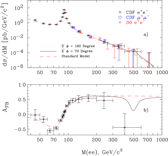
Figure 20: Dilepton mass spectrum from the Drell-Yan process from the CDF and D0 experiments at the Tevatron for Run 1.

4 The W boson

In the on-shell renormalisation scheme $\sin^{2}\!\theta_{\mathrm{W}}=1-m_{\mathrm{W}}^{2}/m_{\mathrm{Z}}^{2}$, so that precise measurements of the W and Z masses give directly the weak mixing angle. An accurate measurement of the W-boson mass gives a rather precise indirect estimate of the Higgs boson mass in the SM, from electroweak radiative corrections. The W-boson decays weakly into either a quark-antiquark pair or a lepton and its corresponding neutrino. The partial leptonic decay width is given by [49]

$$\Gamma(\mbox{$\mathrm{W}\rightarrow\mathrm{e\overline{\nu}_{e}}$})=\frac{G_{\mathrm{F}}m_{\mathrm{W}}^{3}}{6\pi\sqrt{2}}(1+\delta^{sm})=227.0\pm 0.3\hskip 2.84544pt\hbox{\rm Me\kern-1.00006ptV},\ \$$ (41)

where the error is dominated by the present uncertainty in $m_{\mathrm{W}}$ (see below). If the values of $G_{\mathrm{F}}$ and $m_{\mathrm{W}}$ are used to determine the SM value of $\Gamma(\mbox{$\mathrm{W}\rightarrow\mathrm{e\overline{\nu}_{e}}$})$, then the electroweak corrections $\delta^{sm}$ are small ($\simeq$ -0.35 $\%$), because the bulk of the corrections are absorbed in $G_{\mathrm{F}}$ and $m_{\mathrm{W}}$. The partial width to $q\bar{q}$ final states, for massless quarks, is given by

$$\Gamma(\mbox{$\mathrm{W}\rightarrow q_{i}\overline{q}_{j}$})=f_{QCD}\Gamma(\mbox{$\mathrm{W}\rightarrow\mathrm{e\overline{\nu}_{e}}$})\mid V_{ij}\mid^{2}.\ \$$ (42)

where f_QCD = 3(1 + $\alpha_{\rm{s}}{\rm(m_{\mathrm{W}})}/\pi$ + 1.409($\alpha_{\rm{s}}{\rm(m_{\mathrm{W}})}/\pi$)² + …) is a QCD colour correction factor (similar to eqn. 22) and V_ij is the Cabibbo-Kobayashi-Maskawa [50, 51](CKM) matrix element. The total width $\Gamma_{\mathrm{W}}$ in the SM is given by

$$\Gamma_{\mathrm{W}}=(3+2f_{QCD})\Gamma(\mbox{$\mathrm{W}\rightarrow\mathrm{e\overline{\nu}_{e}}$})=2.0986\pm 0.0028\hskip 2.84544pt\hbox{\rm Ge\kern-1.00006ptV},\ \$$ (43)

where the uncertainty from $\alpha_{\rm{s}}{\rm(m_{\mathrm{W}})}$ (=0.121 $\pm$ 0.002) is 1.0 MeV, and that from $m_{\mathrm{W}}$ is 2.6 MeV.

The main $q\bar{q}$ decay modes are $u\bar{d}$ and $c\bar{s}$.The $q\bar{q}$ branching ratio thus gives mainly constraints on the matrix elements V_ud and V_cs. Since the former is well known from other measurements, the $q\bar{q}$ mode can be used to give V_cs. The decay branching ratios (as measured at LEP [8, 52]) are given in table 15. In the combination procedure, common systematic errors (e.g. from the 4-jet QCD background) are taken into account. The data allow sensitive tests of the validity of lepton universality of the weak charged-current, at a level of better than 3$\%$:

$$B(\mbox{$\mathrm{W}\rightarrow\mu\overline{\nu}_{\mu}$})/B(\mbox{$\mathrm{W}\rightarrow\mathrm{e\overline{\nu}_{e}}$})=1.000\pm 0.021,$$

$$B(\mbox{$\mathrm{W}\rightarrow\tau\overline{\nu}_{\tau}$})/B(\mbox{$\mathrm{W}\rightarrow\mathrm{e\overline{\nu}_{e}}$})=1.052\pm 0.029,$$

$$B(\mbox{$\mathrm{W}\rightarrow\tau\overline{\nu}_{\tau}$})/B(\mbox{$\mathrm{W}\rightarrow\mu\overline{\nu}_{\mu}$})=1.052\pm 0.028.$$ (44)

Assuming lepton universality, B($\mathrm{W}\rightarrow\ell\overline{\nu}_{\ell}$) = 10.69 $\pm$ 0.06 (stat) $\pm$ 0.07 (syst)$\%$, compatible with the SM value of 10.82$\%$.

The decay branching ratios have also been extracted at hadron colliders by measuring the ratio

$$R=\frac{\sigma(p\bar{p}\rightarrow W\rightarrow\mbox{${e\overline{\nu}_{e}}$})}{\sigma(p\bar{p}\rightarrow Z\rightarrow\mathrm{e}^{+}\mathrm{e}^{-})},\\$$ (45)

which can be written as

$$R=\frac{\sigma(p\bar{p}\rightarrow W+..)}{\sigma(p\bar{p}\rightarrow Z+..)}\frac{\Gamma_{\mathrm{Z}}}{\Gamma(Z\rightarrow\mathrm{e}^{+}\mathrm{e}^{-})}\frac{\Gamma(\mbox{$\mathrm{W}\rightarrow\mathrm{e\overline{\nu}_{e}}$})}{\Gamma_{\mathrm{W}}}\ \ .$$ (46)

Using the measured value of the Z leptonic branching fraction from LEP, and the SM theoretical calculation of the ratios of the W and Z cross-sections ($\simeq$ 3.3), the CDF and D0 Tevatron measurements give [53] BR($\mathrm{W}\rightarrow\mathrm{e\overline{\nu}_{e}}$) = (10.43 $\pm$ 0.25)$\%$. In this, the total systematic uncertainty is 0.23$\%$, with 0.19$\%$ coming from the QED uncertainties in the acceptance calculations and in the $\sigma_{W}$/$\sigma_{Z}$ ratio.

The combined LEP and Tevatron value is BR($\mathrm{W}\rightarrow\mathrm{e\overline{\nu}_{e}}$) = (10.66 $\pm$ 0.09)$\%$. In terms of the CKM matrix elements

$$\frac{1}{BR(\mbox{$\mathrm{W}\rightarrow\mathrm{e\overline{\nu}_{e}}$})}=3+f_{QCD}\sum_{ij}\mid V_{ij}\mid^{2},$$ (47)

where the sum is over i=(u,c) and j=(d,s,b). This gives

$$\sum_{ij}\mid V_{ij}\mid^{2}=2.044\pm 0.024,$$ (48)

where an error of 0.001 comes from $\delta\alpha_{\rm{s}}{\rm(m_{\mathrm{W}})}$ and the rest is from $\delta$BR($\mathrm{W}\rightarrow\mathrm{e\overline{\nu}_{e}}$). Using the experimental value for the sum of all elements except $\mid V_{cs}\mid^{2}$, namely 1.0477 $\pm$ 0.0074 [2], the value

$$\mid V_{cs}\mid=0.998\pm 0.013$$ (49)

can be extracted. In this, the uncertainty from the measured W branching fraction is $\pm$ 0.013, the input CKM uncertainty is $\pm$ 0.004, and that from $\alpha_{\rm{s}}{\rm(m_{\mathrm{W}})}$ is negligible.

Alternatively, the combined leptonic branching ratio from LEP and the Tevatron, together with the SM value of $\Gamma(\mbox{$\mathrm{W}\rightarrow\mathrm{e\overline{\nu}_{e}}$})$, can be used to make an indirect measurement of the W-boson width of $\Gamma_{\mathrm{W}}$ = 2.130 $\pm$ 0.017 GeV. This value is 1.8$\sigma$ from the SM prediction given in eqn.(43).

4.1 Mass and width of the W boson

The measurements of the mass of the W boson, $m_{\mathrm{W}}$, have been made at proton-antiproton colliders (by UA2 [54] at CERN and CDF [55] and D0 [56] at the Tevatron) and at LEP (by ALEPH [57], DELPHI [58], L3 [59] and OPAL [60], and references therein), with updates reported in [8].

4.1.1 Mass and width of the W boson from hadron colliders

For measurements of $m_{\mathrm{W}}$ at hadron colliders the purely hadronic W decay mode suffers from too much background and only the electron and muon leptonic decays have been used. The W-bosons are produced by the reaction $q_{1}+\bar{q_{2}}\rightarrow$ W $\rightarrow$ e($\mu$) + $\nu_{e}$($\nu_{\mu}$). The event topology selected is an isolated electron or muon, plus the residual hadronic system from the collision. The neutrino is not detected and can give a sizeable missing transverse energy/momentum. Since a large fraction of the longitudinal energy and momentum escapes detection in the forward regions of detectors in, or close to, the beam-pipe, only the plane perpendicular to the beam-axis can be used to impose energy-momentum constraints. Measurement is made of the lepton energy/momentum, plus that of the recoil jet (${\bf u}$); see fig. 21. From these quantities the transverse mass, $m_{\mathrm{trans}}$, is constructed

$$m_{\mathrm{trans}}^{2}=2p_{T}^{\ell}p_{T}^{\nu}(1-\cos\Delta\phi),$$ (50)

where p${}_{T}^{\ell}$ and p${}_{T}^{\nu}$ are the charged lepton and neutrino transverse momenta and $\Delta\phi$ is their azimuthal separation. The neutrino component is reconstructed from measurement of the recoil ${\bf u}$, and the understanding of this recoil system is crucial to the analysis. The Z boson is produced by the process $q+\bar{q}\rightarrow$ Z $\rightarrow$ $\mathrm{e}^{+}\mathrm{e}^{-}$ ($\mu^{+}\mu^{-}$). A study of Z boson production and leptonic decays is of great importance, both in calibrating the energy/momentum scale and in understanding the p_T production spectrum of heavy bosons. The leptonic decays of the J/$\Psi$ boson are also useful in the scale calibrations. Another important systematic uncertainty is the imprecision in the knowledge of the parton density functions (PDFs) in the incident proton and antiproton. The lepton transverse energy spectra have also be used to determine $m_{\mathrm{W}}$, but these of course are correlated to $m_{\mathrm{trans}}$.

All the data from the Tevatron Run 1, which finished in 1995 and yielded an integrated luminosity of about 110 pb^-1, have been analysed. An example of a transverse mass distribution, from the $\mathrm{W}\rightarrow\mathrm{e\overline{\nu}_{e}}$ decay, is given in fig. 22. The results from the Tevatron CDF and D0 experiments, and the earlier UA2 experiment at CERN are given in table 16(from  [61]), together with the average value. In combining the Tevatron data, a 25 MeV common systematic error is used. This covers common uncertainties in the PDFs, W-width and QED corrections.

The W width is extracted by making a likelihood fit to the large transverse mass part of the $m_{\mathrm{trans}}$ spectrum. This region is rather insensitive to detector resolution effects, which fall off in an approximately Gaussian manner, but is sensitive to the W width. The combined CDF result from the electron and muon channels [62], using the range $m_{\mathrm{trans}}\mathbin{\mskip 5.0mu plus 5.0mu\raise 1.0pt\hbox{$>$}\kern-8.0pt\lower 3.0pt\hbox{$\sim$}\mskip 5.0mu plus 5.0mu}$ 120 GeV, is $\Gamma_{\mathrm{W}}$ = 2.05 $\pm$ 0.10 $\pm$ 0.08 GeV. For D0 (see  [61]) the range 90 $\mathbin{\mskip 5.0mu plus 5.0mu\raise 1.0pt\hbox{$<$}\kern-8.0pt\lower 3.0pt\hbox{$\sim$}\mskip 5.0mu plus 5.0mu}m_{\mathrm{trans}}\mathbin{\mskip 5.0mu plus 5.0mu\raise 1.0pt\hbox{$<$}\kern-8.0pt\lower 3.0pt\hbox{$\sim$}\mskip 5.0mu plus 5.0mu}$ 200 GeV is used for the electron channel, giving $\Gamma_{\mathrm{W}}$ = 2.23 $\pm$ 0.14 $\pm$ 0.09 GeV. Assuming a common systematic uncertainty of 50 MeV, a combination of the Tevatron results gives $\Gamma_{\mathrm{W}}$= 2.11 $\pm$ 0.11 GeV.

Figure 21: Kinematics of W decay in the plane transverse to the beam direction. The recoil energy vector of the n detected hadrons is ${\bf u}$ = $\sum_{i=1}^{n}$ $E_{T}^{i}$.

Table 15: W boson branching ratios from measurements at LEP. For the $q\bar{q}$ mode lepton universality is assumed.

• decay mode	branching ratio $\%$
  $q\bar{q}$	$67.92\pm 0.27$
  ${e\overline{\nu}_{e}}$	$10.54\pm 0.17$
  ${\mu\overline{\nu}_{\mu}}$	$10.54\pm 0.16$
  ${\tau\overline{\nu}_{\tau}}$	$11.09\pm 0.22$

Table 16: W mass measurements from hadron colliders.

• experiment	decay modes used	$m_{\mathrm{W}}$ (GeV)
  UA2	$\mathrm{W}\rightarrow\mathrm{e\overline{\nu}_{e}}$,$\mathrm{W}\rightarrow\mu\overline{\nu}_{\mu}$	$80.360\pm 0.370$
  CDF	$\mathrm{W}\rightarrow\mathrm{e\overline{\nu}_{e}}$,$\mathrm{W}\rightarrow\mu\overline{\nu}_{\mu}$	$80.433\pm 0.079$
  D0	$\mathrm{W}\rightarrow\mathrm{e\overline{\nu}_{e}}$	$80.483\pm 0.084$
  average		$80.454\pm 0.060$

Figure 22: Transverse mass distribution from the CDF experiment for the decay $\mathrm{W}\rightarrow\mathrm{e\overline{\nu}_{e}}$. The points represent the data and the histogram shows the Monte Carlo simulation of the signal and background. The region used to fit $m_{\mathrm{W}}$ is shown.

4.1.2 Mass and width of the W boson at LEP

One of the main purposes behind increasing the energy for LEP 2 above the W-pair threshold (around 161 GeV) was to study the production and decay properties of the W boson. The lowest-order diagrams for producing W pairs are shown in fig. 23. These diagrams are collectively known as CC03 diagrams, as the three diagrams are charged-current interactions. They consist of t-channel neutrino exchange and s-channel exchange of a photon or Z boson. In the Standard Model there are large cancellations between these diagrams, and thus measurement of the production cross-section of $\mathrm{e}^{+}\mathrm{e}^{-}\rightarrow\mathrm{W^{+}W^{-}}$ is a very sensitive test of the SM.

The reaction $\mathrm{e}^{+}\mathrm{e}^{-}\rightarrow\mathrm{W^{+}W^{-}}$ can be extracted relatively cleanly at LEP and all the decay modes of the W can be used. Thus the samples analysed consist of fully hadronic final states (46 %), semileptonic final states (44 %) and purely leptonic final states (10 %). The purely leptonic and semileptonic final states can be selected relatively cleanly from background, but there is a potentially sizeable background from $\mathrm{e}^{+}\mathrm{e}^{-}\rightarrow{\rm q}\overline{\rm q}(\gamma)$ in the fully hadronic final state. The cross-sections for these CC03 processes have been measured and combined by the four LEP experiments. Small corrections have to be applied for other 4-fermion final states with the same topologies. The results are shown in fig. 24. It can be seen that the data are compatible with the SM predictions, which at the highest energies have an uncertainty of about 0.5%. The results clearly demonstrate the existence of the triple-gauge boson couplings.

The first data taken in the LEP 2 phase consisted of a dedicated run at $\sqrt{s}$ = 161 GeV; just above the W-pair threshold. The cross-section in this region is very sensitive to $m_{\mathrm{W}}$. Hence, from the measurement of the cross-section, $m_{\mathrm{W}}$ may be extracted; assuming the validity of the Standard Model. The indirect determination of $m_{\mathrm{W}}$ by this method is given in table 17. The contribution of the 2% uncertainty in the SM predictions gives a 34 MeV component to the systematic error.

The threshold method is valid in the SM. A comparison of the LEP data, averaged over all cms energy values, and taking into account common systematic uncertainties, gives a value of R_WW = 0.998 $\pm$ 0.009 for the ratio of the measured cross-sections to the SM predictions. These are from the YFSWW generator [63], which employs a double-pole approximation approach and has $\cal{O}(\alpha)$ electroweak corrections. An alternative model, RACOONWW [64], gives a very compatible value, namely R_WW = 1.000 $\pm$ 0.009. These results show that the data are consistent with the SM up to the highest available energies.

A much more accurate determination of $m_{\mathrm{W}}$ has been made using direct reconstruction of the W mass in the reaction $\mathrm{e}^{+}\mathrm{e}^{-}\rightarrow\mathrm{W^{+}W^{-}}$. The purely leptonic mode yields a rather large error, so emphasis is placed on the semi-leptonic ($q\bar{q}\mbox{${\ell\overline{\nu}_{\ell}}$}$) and fully hadronic ($q\bar{q}q\bar{q}$) final states. For the $q\bar{q}q\bar{q}$ analysis events are selected which contain four (or more) jets. Again $\mathrm{e}^{+}\mathrm{e}^{-}\rightarrow{\rm q}\overline{\rm q}(\gamma)$ is the largest background. In a four-jet final state there are three possible combinations with which the jets can be paired into two W bosons. However, in practice only one, or sometimes two, are compatible with the previously known value of $m_{\mathrm{W}}$. The experimental resolution on the invariant mass of a pair of jets is typically 5-10 GeV. Some fraction of the jet energy is generally not detected. The resolution can be greatly improved (to $\simeq$ 1 GeV) by using a kinematic fit in which energy-momentum constraints (4C-fit) are imposed. This requires a rather precise knowledge of the LEP beam energy, and the uncertainty on this is one of the main systematic errors.

For the $q\bar{q}\mbox{${\ell\overline{\nu}_{\ell}}$}$ channel the assignment of the jets to the parent W boson is straightforward. The lepton is well measured in the case of electron and muon decays; however, there is a missing neutrino. In this case the kinematic fit gives only one constraint, except if, as is often the case, it is assumed that the mass of the W from the $q\bar{q}$ and ${\ell\overline{\nu}_{\ell}}$ systems are equal; in which case it becomes a 2C-fit. For the $q\bar{q}\mbox{${\tau\overline{\nu}_{\tau}}$}$ channel the leptonic part is not constrained, and all the information on $m_{\mathrm{W}}$ comes from the $q\bar{q}$ system, which is again scaled to the LEP beam energy. The W-boson width, $\Gamma_{\mathrm{W}}$, is also extracted in these fits, and has only a small correlation with $m_{\mathrm{W}}$.

A variety of different sophisticated techniques are used to extract $m_{\mathrm{W}}$ from these event samples. The most straightforward method is the convolution method, in which the theoretical Breit-Wigner form  for the invariant mass of the W decay products is convoluted with the experimental resolution on this quantity. Both the W mass and width can be determined. The method must be ‘calibrated’ by fitting Monte Carlo samples of known mass (or masses). The linearity of the method with respect to the determination of $m_{\mathrm{W}}$, and also the validity of the assigned statistical uncertainty, must both be studied. An alternative is the Monte Carlo reweighting method in which Monte Carlo events are reweighted such that they correspond to a series of different generated masses. The value of the W mass which best fits the data is found. The distribution which is fitted is the invariant mass of the W-decay products, plus possibly other distributions which are sensitive to $m_{\mathrm{W}}$. In both these methods it is usual to force the mass of the decay products from the two W-pairs in the kinematic fit to be equal. An ideogram method has also been used in which all jet pairings are taken, and the equal mass constraint is not imposed. A likelihood function is then constructed for each event, as a function of $m_{\mathrm{W}}$, and these likelihoods are combined to give the best value from all the events.

A particular problem is the $\mathrm{e}^{+}\mathrm{e}^{-}\rightarrow{\rm q}\overline{\rm q}(\gamma)$ background in $q\bar{q}q\bar{q}$. This background must either be removed by suitable selection cuts, or taken into account by weighting the events in such a way that the probabilility that they are signal or background events is taken into account, The jet fragmentation process is potentially a common systematic uncertainty between channels and between the different LEP experiments. The effects of initial state radiation (ISR) are also a common uncertainty. Considerable effort has been made to understand these processes. In the fully hadronic final states there is the additional potential problem of ‘cross-talk’ between the decay products of the two W’s. This can arise through colour reconnection, as, for example, ‘strings’ can be formed between the quarks and gluons from the different W’s. These effects can only be computed in QCD at the perturbative level, where they are small. However, it is in the region of soft particles that the effects are expected to be more pronounced. This is in the domain of Monte Carlo models, and several options for models exist. These can yield shifts in $m_{\mathrm{W}}$ up to about 100 MeV, but the bulk of the models give shifts $\mathbin{\mskip 5.0mu plus 5.0mu\raise 1.0pt\hbox{$<$}\kern-8.0pt\lower 3.0pt\hbox{$\sim$}\mskip 5.0mu plus 5.0mu}$ 50 MeV. Ideally it is desirable to find measurable quantities, which are insensitive to $m_{\mathrm{W}}$, but which are sensitive to the parameters of the model. The measurements of these parameters, within the context of the model, can then be used to ‘calibrate’ the model by finding the shifts in the values of $m_{\mathrm{W}}$ corresponding to the measured model parameter range. One promising possibility is to measure the particle flow (i.e. the density of particles) between jets coming from different W-bosons, and compare it with that measured between jets from the same W. From such measurements it is hoped that the colour reconnection parameters in the various models can be constrained. In practice these attempts are complicated by the pairing ambiguities in jets, and the fact that the 4 jets in the final state are generally not coplanar.

There can also be Bose Einstein correlations (BEC) between the decay products of the two W’s. Such correlations are well known in multiparticle final states and lead to an enhancement in the invariant mass distribution of like-sign bosons near threshold. In principle such correlations can arise between, for example, pairs of pions from different W-bosons. Studies of differences in the hadronic systems of hadrons from jets in a semi-leptonic W decay (where there can only be BEC between the W decay products) and those in fully-hadronic decays (which might also have BEC between decay products of different W’s) are being carried out. There are also several options in the Monte Carlo simulation models of BEC. However, it is worth stressing that, in terms of the underlying quantum mechanical effects, all the existing models are somewhat ad hoc. The technique used is to modify the four-momenta of pairs of particles, and to compensate the overall energy-momentum conservation either locally or globally.

The colour reconnection and BEC can both lead to ‘cross-talk’ effects, and thus an apparent shift in $m_{\mathrm{W}}$ and $\Gamma_{\mathrm{W}}$. They are collectively referred to as final state interaction (FSI) effects. They constitute one of the largest systematic uncertainties in the $q\bar{q}q\bar{q}$ final state. Investigations have shown that all the experiments are equally sensitive to these effects, and so the same common systematic uncertainties for these effects are used in making a LEP combination.

The measurements of the W mass and width from the LEP experiments are combined, taking into account the common systematic errors. For the mass, the main errors common to both the $q\bar{q}\mbox{${\ell\overline{\nu}_{\ell}}$}$ and $q\bar{q}q\bar{q}$ are the fragmentation uncertainty (17 MeV), initial and final state radiation (8MeV), and the LEP beam energy (17 MeV; see below). The colour reconnection and Bose Einstein correlation errors are currently assigned to be 40 and 25 MeV respectively for the $q\bar{q}q\bar{q}$ channel. These get reduced to 11 and 7 MeV in the combined result, as the $q\bar{q}q\bar{q}$ carries less weight in the combination. The weight of the $q\bar{q}q\bar{q}$ channel is 27$\%$. This is essentially due to the relatively large size of these effects, since both channels would give roughly the same weight without these FSI errors. For $\Gamma_{\mathrm{W}}$, the colour reconnection and Bose Einstein correlation errors are taken to be 65 and 35 MeV repectively. The results for the mass and width for the four LEP experiments are shown in fig. 25. The combined LEP results for $m_{\mathrm{W}}$ from the threshold method, and for the different decay channels for the direct reconstruction method, are given in table 17. The overall LEP combined results for $m_{\mathrm{W}}$ and $\Gamma_{\mathrm{W}}$ are

$$m_{\mathrm{W}}=80.450\pm 0.039\hskip 5.69046pt{\rm GeV}$$

$$\Gamma_{\mathrm{W}}=2.150\pm 0.091\hskip 5.69046pt{\rm GeV}.$$ (51)

For $\Gamma_{\mathrm{W}}$, the combined statistical and systematic errors are 0.068 and 0.060 GeV respectively.

The difference between the fully hadronic and semi-leptonic mass measurements can also be extracted. A significant non-zero value for $\Delta m_{\mathrm{W}}$ could be indicative of large FSI effects in the $q\bar{q}q\bar{q}$ channel. The FSI errors are neglected in making this difference, and this gives $\Delta m_{\mathrm{W}}(q\bar{q}q\bar{q}-q\bar{q}\mbox{${\ell\overline{\nu}_{\ell}}$})$ = +9 $\pm$ 44 MeV, well compatible with zero. However, it should be noted that this difference is not precise enough to be sensitive to shifts of the size of the FSI errors currently assigned. Further efforts are being made in devising track selection procedures which are less sensitive to FSI effects; for example, by removing or de-weighting low momentum tracks and/or tracks at wide angles to the W jet-axes.

The LEP beam energy in the LEP 2 range has an uncertainty of about 20 MeV. This arises because the method of resonant depolarisation only works up to about 60 GeV beam energies. Hence extrapolations need to be made, and this significantly increases the uncertainty. The main method is to use 16 NMR devices which were installed around the ring and to use the flux-loop method, which measures the total field seen by the beam, as a check of the linearity of the extrapolation.

4.2 World average values of the W boson mass and width

The combined Tevatron and LEP measurements of $m_{\mathrm{W}}$ and $\Gamma_{\mathrm{W}}$ give

$$m_{\mathrm{W}}=80.451\pm 0.033\hskip 5.69046pt{\rm GeV},$$

$$\Gamma_{\mathrm{W}}=2.134\pm 0.069\hskip 5.69046pt{\rm GeV}.$$ (52)

This direct $m_{\mathrm{W}}$ result is compared to more indirect determinations in fig. 26. It can be seen that the NuTeV value, and to a lesser extent the indirect electroweak fit results (these are both discussed below), favour lower values of $m_{\mathrm{W}}$. The result for $\Gamma_{\mathrm{W}}$ can be used to make an estimate of the W mass, by utilising the SM relationship (43). This gives $m_{\mathrm{W}}$ = 80.90 $\pm$ 0.87 GeV, which is consistent with the direct measurement, but has a sizeable error.

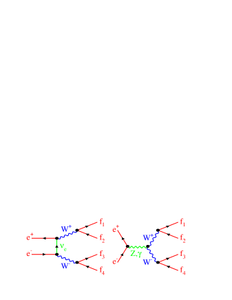
Figure 23: The three lowest-order charged current (CC03) diagrams for $\mathrm{e}^{+}\mathrm{e}^{-}\rightarrow\mathrm{W^{+}W^{-}}$.

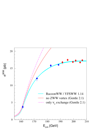
Figure 24: Cross-section for the CC03 process $\mathrm{e}^{+}\mathrm{e}^{-}\rightarrow\mathrm{W^{+}W^{-}}$, as a function of cms energy.

Table 17: W mass measurements from LEP. The components of the errors from statistics and systematics are shown, with the contribution of the LEP energy uncertainty shown separately. The last two results have a correlation coefficient of 0.28.

• method	$m_{\mathrm{W}}$ (GeV)	stat. error.	syst. error	LEP error
  threshold	80.40	0.20	0.07	0.03
  $q\bar{q}\mbox{${\ell\overline{\nu}_{\ell}}$}$	80.448	0.033	0.028	0.017
  $q\bar{q}q\bar{q}$	80.457	0.030	0.054	0.017

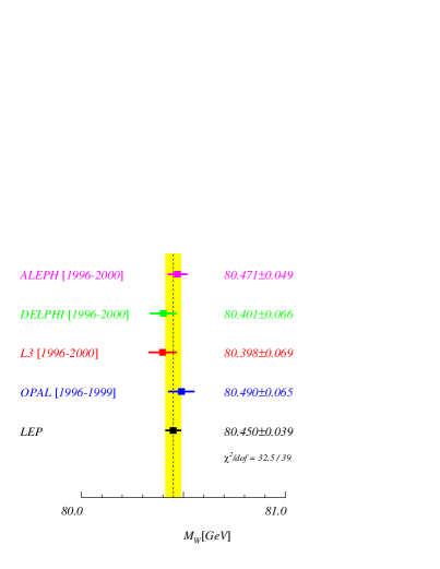
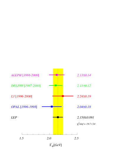
Figure 25: Mass and width of the W boson as measured by the LEP experiments. The combined LEP average is also shown.

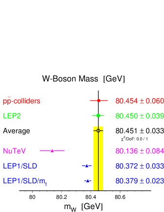
Figure 26: Comparison of direct and indirect determinations of $m_{\mathrm{W}}$.

5 The running of $\alpha$

The fine structure constant is known at q${}^{2}\simeq$ 0 with the impressive relative precision of 4x10^-9. However, what is important for the interpretation of heavy gauge boson results is the value at a scale $m_{\mathrm{Z}}$, $\alpha(m_{\mathrm{Z}})$. The running of $\alpha$(s) is given by eqn.(15). The running component $\Delta\alpha(s)$ = $-\Pi_{\gamma\gamma}(s)$, where $\Pi_{\gamma\gamma}$ is the photon self-energy. At s = $m_{\mathrm{Z}}^{2}$ the leptonic contribution $\Delta\alpha_{lept}$ can be computed analytically, and is known to third-order. The top-quark contribution, $\Delta\alpha_{top}$, is well known if $m_{\mathrm{t}}$ is specified ($\simeq$- 0.00007). The remaining hadronic part $\Delta\alpha_{had}^{(5)}$ cannot be calculated entirely from QCD because of ambiguities in defining the light quark masses m_u and m_d, and also the inherent non-perturbative nature of the problem at small energy scales. The largest uncertainties come from this term. Instead, use is made of the data on

$$R_{had}(s)=\frac{\sigma(\mathrm{e}^{+}\mathrm{e}^{-}\rightarrow\mathrm{hadrons})}{\sigma(\mathrm{e}^{+}\mathrm{e}^{-}\rightarrow\mu^{+}\mu^{-})},$$ (53)

from which one can compute

$${\rm Re}\Pi_{\gamma\gamma}(s)=\frac{\alpha{\rm s}}{3\pi}P\int\frac{R_{had}(s^{{}^{\prime}})}{s^{{}^{\prime}}(s^{{}^{\prime}}-s)}ds{{}^{\prime}}\ \ .$$ (54)

Most of the sensitivity is to $R_{had}$ at low values of $\sqrt{s}$, below about 10 GeV. In practice, there are difficulties in evaluating the integral:-

• from the resonant structure in the data ($\rho$,$\omega$,J/$\psi$, $\Upsilon$),

• some data are not very accurate (e.g. large systematic errors) and old (not always enough information is given),

• somewhat arbitrary choices need to be made in the use of the data (e.g. the form of local parameterisation, interpolation or fit, how to deal with inconsistent data and how to cross thresholds etc.).

Figure 27: Recent estimates of $\Delta\alpha^{(5)}_{had}(m_{\mathrm{Z}})$. Those which rely mostly on experimental data are shown as solid circles, while the more theory-driven estimates are shown as open circles.

Figure 28: Measurements of R by BES and other experiments: (a) over the cms energy range 1 to 5 GeV and (b) around the charm threshold.

Fig.27 shows some of the more recent determinations [65, 66, 67, 68, 69, 70, 71, 72, 73], starting with the previous value used by the LEP Electroweak Working Group, namely $\Delta\alpha^{(5)}_{had}(m_{\mathrm{Z}})$ = 0.02804 $\pm$ 0.00065. Only the most recent of these use the new data from Novosibirsk around the $\rho$ resonance and the BES-2 data for the very important region from 2-5 GeV; see fig.28. For the fits below, the value used is [72]

$$\Delta\alpha^{(5)}_{had}(m_{\mathrm{Z}})=0.02761\pm 0.00036.$$ (55)

This incorporates the recent data, and experimental data are used below 12 GeV and third-order perturbative QCD used above.

Some other determinations are more theory-driven, and use perturbative QCD to low $\sqrt{s}$, justifying this by the success of extracting $\alpha_{\rm{s}}{\rm(m_{\mathrm{Z}})}$ from $\tau$-decays. As an example, a recent more theory-driven determination, which also includes results from BES, of $\Delta\alpha^{(5)}_{had}(m_{\mathrm{Z}})$ = 0.02747 $\pm$ 0.00012 [73], is also used below.

5.1 muon (g-2)

The anomolous magnetic moment of the muon, which is defined as

$$a_{\mu}=\frac{g_{\mu}-2}{2},$$ (56)

has been measured at Brookhaven by experiment E821 [74] to remarkable precision, giving the updated average value

$$a_{\mu}({\rm expt})=(11659203\pm 15)10^{-10}.$$ (57)

At the time the E821 result was announced the SM estimate was such that

$$a_{\mu}({\rm expt})-a_{\mu}({\rm SM})=(43\pm 16)10^{-10},$$ (58)

a difference of 2.6 standard deviations. The SM computation is rather similar to that for $\alpha(m_{\mathrm{Z}})$, with contributions from QED, weak effects and also hadronic effects. Since then, a sign error in the computation of part of the so-called light by light term, which is part of the hadronic term and about 5.6 10^-10 in magnitude, was found[75]. With this corrected

$$a_{\mu}({\rm expt})-a_{\mu}({\rm SM})=(26\pm 16)10^{-10},$$ (59)

so the difference is reduced to 1.6 standard deviations. This has significantly reduced the flow of papers interpreting the difference.

6 Other electroweak measurements

6.1 The top quark

The discovery of the top quark at the Fermilab Tevatron, by the CDF [76] and D0 [77] Collaborations, is clearly of fundamental importance in the field of electroweak physics. The parameter which is most important in the context of this review is the mass of the top-quark, $m_{\mathrm{t}}$. Since the top-quark is so massive it decays very quickly on the time-scale of the hadronisation processes. Hence the interpretation of the top-quark mass is more straightforward than that of the lighter quark masses. The main decay mode is t $\rightarrow$ Wb, so the event classification of the produced ${\mathrm{t}\overline{\mathrm{t}}}$ pair depends on the decay modes of the W bosons. Both CDF and D0 measure the mass in both the dilepton and lepton plus jets channels, with the latter being the more accurate. The results for the top-quark pole mass are $m_{\mathrm{t}}$ = 172.1 $\pm$ 7.1 GeV for CDF [78] and $m_{\mathrm{t}}$ = 176.1 $\pm$ 6.6 GeV for D0 [79]. Typical systematic uncertainties on these measurements are $\simeq$ 5 GeV. A combination of the measured values gives [39]

$$m_{\mathrm{t}}=174.3\pm 5.1\ \ \hbox{\rm Ge\kern-1.00006ptV}.$$ (60)

6.2 Atomic parity violation

Measurements of Atomic Parity Violation (APV) in Cesium [80, 81] are also used to give information on the weak neutral current. The nuclear spin-independent weak interaction of an electron with the nucleus is of the form H $\propto G_{\mathrm{F}}\rho(r)$Q_W, where $\rho$(r) is the nuclear density. The quantity measured is the weak charge

$$Q_{W}(Z,N)=-2[C_{1u}(2Z+N)+C_{1d}(Z+2N)],$$ (61)

where Z and N are the number of protons and neutrons in the nucleus and C_1q = 2$a_{\rm{e}}v_{\rm{q}}$ is defined in terms of the electron axial-vector and quark vector couplings at a scale q${}^{2}~{}\simeq$ 0. So, to leading order,

$$C_{1u}=\rho(-\frac{1}{2}+\frac{4}{3}\sin^{2}\!\theta_{\mathrm{W}}),$$

$$C_{1d}=\rho(\frac{1}{2}-\frac{2}{3}\sin^{2}\!\theta_{\mathrm{W}}).$$ (62)

Measurements have also been made for Thallium, but there are outstanding questions on theoretical corrections [82, 83, 84], which have only recently been addressed for Cesium. Using the new evaluation of the 6s-7s transition, the corrected experimental result for Cesium (Z=55,N=78) is [84]

$$Q_{\rm W}({\rm Cs})=-72.39\pm 0.29(expt)\pm 0.51(theory)=-72.39\pm 0.59.$$ (63)

6.3 Neutrino neutral to charged current ratio

Measurements of the neutral-current (NC) to charged-current (CC) ratio in deep inelastic $\nu$($\bar{\nu}$)-nucleon scattering can be used to make a determination of the weak mixing angle. Note that this is a t-channel process, in contrast to $\mathrm{e}^{+}\mathrm{e}^{-}\rightarrow{\rm f}\overline{\rm f}$, which is s-channel (for f$\neq$e).

The tree-level Lagrangian for weak neutral current neutrino-quark scattering is

$${\cal{L}}=-\frac{G_{\mathrm{F}}\rho_{0}}{\sqrt{2}}[\bar{\nu}\gamma^{\mu}(1-\gamma^{5})\nu][\epsilon^{q}_{L}\bar{q}\gamma_{\mu}(1-\gamma^{5})q+\epsilon^{q}_{R}\bar{q}\gamma_{\mu}(1+\gamma^{5})q],$$ (64)

where any deviations from $\rho_{0}$ = 1 describe non-standard sources of SU(2) breaking. $\epsilon^{q}_{L,R}$ are the left- and right-handed chiral quark couplings, which contain a term  -Q${}_{q}\sin^{2}\!\theta_{\mathrm{W}}$. For the weak charged current the corresponding couplings are $\epsilon^{q}_{L}$ = t${}^{3}_{q}$ and $\epsilon^{q}_{R}$ = 0. Thus measurement of the NC/CC ratio gives values of $\rho_{0}$ and $\sin^{2}\!\theta_{\mathrm{W}}$. In the context of the SM, this measurement of $\sin^{2}\!\theta_{\mathrm{W}}$ is equivalent to a measurement of $m_{\mathrm{W}}$, but outside the SM it provides measurements of the weak couplings of light-quarks at a momentum scale far below $m_{\mathrm{Z}}$.

The NC/CC ratio for scattering off an isoscalar nuclear target is

$$R^{\nu(\bar{\nu})}\equiv\frac{\sigma(\nu(\bar{\nu})N\rightarrow\nu(\bar{\nu})X)}{\sigma(\nu(\bar{\nu})N\rightarrow\ell^{-(+)}X)}$$

$$=g_{L}^{2}+r^{(-1)}g_{R}^{2},$$ (65)

where r = $\sigma$( $\bar{\nu}$N $\rightarrow\ell^{+}$X)/ $\sigma$( $\nu$N $\rightarrow\ell^{-}$X) $\simeq$ 0.5 and

$$g_{L}^{2}=(\epsilon_{L}^{u})^{2}+(\epsilon_{L}^{d})^{2}=\frac{1}{2}-\sin^{2}\!\theta_{\mathrm{W}}+\frac{5}{9}\sin^{4}\!\theta_{\mathrm{W}}$$

$$g_{R}^{2}=(\epsilon_{R}^{u})^{2}+(\epsilon_{R}^{d})^{2}=\frac{5}{9}\sin^{4}\!\theta_{\mathrm{W}}.$$ (66)

To reduce the dependence on the quark-density functions, and the contribution of strange and other sea-quarks, the combination (Paschos and Wolfenstein [85])

$$R^{PW}=\frac{R^{\nu}-rR^{\bar{\nu}}}{1-r}=g_{L}^{2}-g_{R}^{2}=\frac{1}{2}-\sin^{2}\!\theta_{\mathrm{W}}$$ (67)

is used. The strange sea-quark distribution is studied in dimuon CC events, which are produced from the s$\rightarrow$c reaction.

The most recent, and most precise, result comes from the NuTeV Collaboration who used both neutrino and anti-neutrino beams to give [86]

$$\sin^{2}\!\theta_{\mathrm{W}}=1-m_{\mathrm{W}}^{2}/m_{\mathrm{Z}}^{2}$$

$$\equiv 0.2277\pm 0.0016-0.00022\frac{m_{\mathrm{t}}^{2}-(175~{}\hbox{\rm Ge\kern-1.00006ptV})^{2}}{(50~{}\hbox{\rm Ge\kern-1.00006ptV})^{2}}+0.00032\ln\frac{m_{\mathrm{H}}}{150~{}\hbox{\rm Ge\kern-1.00006ptV}},$$ (68)

where the explicit dependence on $m_{\mathrm{t}}$ and $m_{\mathrm{H}}$ is given. This dependence, which arises from the electroweak radiative corrections to the result, is used in the electroweak fits discussed below. The total uncertainty of 0.0016 has statistical and systematic components of 0.0013 and 0.0009 respectively. The largest systematic uncertainty comes from charm production and the knowledge of the strange sea. The uncertainty in the fraction of the $\nu_{e}$, $\bar{\nu_{e}}$ component of the beam is another important systematic.

This result can be converted into an indirect measurement of the W mass; $m_{\mathrm{W}}$ = 80.136 $\pm$ 0.084 GeV, using $m_{\mathrm{Z}}$ = 91.1875 GeV, $m_{\mathrm{t}}$ = 175 GeV and $m_{\mathrm{H}}$ = 150 GeV. Fig. 26 shows a comparison of the extracted $m_{\mathrm{W}}$ value with the direct measurements. The difference between the world average direct result and that of NuTeV is 300 $\pm$ 92 MeV, almost 3.3 standard deviations apart.

Results are also given for a two-parameter fit to the R^ν and R${}^{\bar{\nu}}$ measurements, namely

$$\rho_{0}=0.9983\pm 0.0040,\hskip 28.45274pt\sin^{2}\!\theta_{\mathrm{W}}=0.2265\pm 0.0031,$$ (69)

with a correlation coefficient of 0.85. Alternatively, the results can be expressed as

$$(g^{eff}_{L})^{2}=0.3005\pm 0.0014,\hskip 28.45274pt(g^{eff}_{R})^{2}=0.0310\pm 0.0011,$$ (70)

with a correlation of -0.02. These are to be compared to the predicted SM values, from a fit to other data, of (g${}^{eff}_{L})^{2}$ = 0.3042 and (g${}^{eff}_{R})^{2}$ = 0.0301. That is, the measured (g${}^{eff}_{L})^{2}$ is lower than the SM expectation by 2.5$\sigma$, whereas (g${}^{eff}_{R})^{2}$ is compatible with the SM.

7 Constraints and tests of the Standard Model

The electroweak data described in the previous sections can be used both to test the self-consistency of the Standard Model and make estimates of the SM parameters.

7.1 Measurements of the weak mixing angle

The various asymmetries discussed in section 3 determine the ratios of the vector to axial-vector couplings of the Z to one or more fermions. From eqn.(26) it can be seen that the measurements thus determine $\sin^{2}\!\theta_{\rm{eff}}^{\rm{f}}$. The value used for reference and comparison is that for leptons, $\sin^{2}\!\theta_{\rm{eff}}^{\rm{lept}}$. Fig. 29 shows a comparison of the various determinations. For the lepton asymmetries ($A^{0,\,\ell}_{\rm{FB}}$, $\mbox{$\cal A_{\ell}$}(\mbox{$\cal P_{\tau}$})$, $\cal A_{\ell}$(SLD)), $\sin^{2}\!\theta_{\rm{eff}}^{\rm{lept}}$ is computed using only the assumption of lepton universality. For the heavy quark measurements ($A^{0,\,{\rm b}}_{\rm{FB}}$,$A^{0,\,{\rm c}}_{\rm{FB}}$) a small correction to get from $\sin^{2}\!\theta_{\rm{eff}}^{\rm{f}}$ to $\sin^{2}\!\theta_{\rm{eff}}^{\rm{lept}}$ is applied, computed from the SM. The overall $\chi^{2}$ gives a probability of 5.9$\%$ for agreement of the results; the main contributions to the $\chi^{2}$ coming from the SLD $A_{\rm{LR}}$ measurement and from $A^{0,\,{\rm b}}_{\rm{FB}}$. As can also be seen from fig. 29, the $A_{\rm{LR}}$ value favours a light value of $m_{\mathrm{H}}$, whereas $A^{0,\,{\rm b}}_{\rm{FB}}$ favours a rather heavy value. The other measurements using quarks also favour a rather heavy Higgs mass, but they are less precise. It can be noted that if $\cal A_{\rm e}$ is computed from $A^{0,\,{\rm b}}_{\rm{FB}}$ and the measured value of $\rm{A_{b}}$, using equation (25), then the value $\sin^{2}\!\theta_{\rm{eff}}^{\rm{lept}}$ = 0.23194 $\pm$ 0.00050 is extracted. This is slightly closer to the values extracted from leptonic asymmetries.

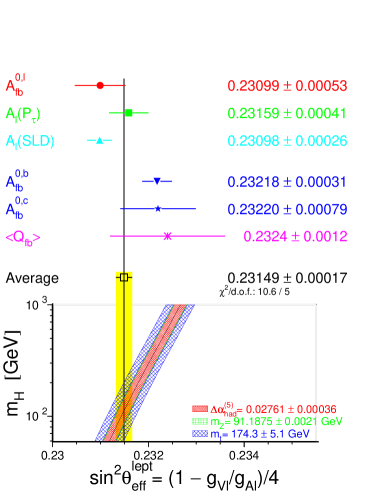
Figure 29: Comparison of the determinations of $\sin^{2}\!\theta_{\rm{eff}}^{\rm{lept}}$. Also shown is the SM expectation as a function of $m_{\mathrm{H}}$, with the bands showing the uncertainties from other SM parameters.

7.2 Global electroweak fits

The electroweak data discussed in this report are used in electroweak fits to test the validity of the Standard Model (see section 2), and to estimate the mass of the important missing ingredient of the SM, the Higgs boson mass. Electroweak quantities are sensitive through propagator and vertex correction terms, which enter (mainly) as $m_{\mathrm{t}}^{2}$ and ln($m_{\mathrm{H}}$). The relative sensitivity is thus much higher for indirect determinations of $m_{\mathrm{t}}$ than $m_{\mathrm{H}}$, but $m_{\mathrm{H}}$ can be significantly constrained, especially if $m_{\mathrm{t}}$ is specified. As already discussed, this led to a prediction of the top-quark mass in advance of its discovery. The present data are now precise enough to significantly constrain the Higgs mass. It is, of course, of considerable interest to compare the limits of direct searches for the Higgs with those from the electroweak fits.

The results of the direct searches for the SM Higgs boson at LEP are briefly discussed in sect. 7.3. The 95$\%$ c.l. lower limit on the Higgs mass is 114.1 GeV, with the possibility of a signal around 115 GeV with a significance of about 2 standard deviations. These values are compared in this section to the values for $m_{\mathrm{H}}$ coming from electroweak fits.

In the electroweak fits the values of the well known ‘constants’ $G_{\mathrm{F}}$ = (1.16637 $\pm$ 0.00001) 10^-5 GeV^-2 [2], $m_{\mathrm{Z}}$ and $\alpha(m_{\mathrm{Z}})$ are used. The fits then give values of $m_{\mathrm{t}}$, $m_{\mathrm{H}}$ and $\alpha_{\rm{s}}{\rm(m_{\mathrm{Z}})}$. The SM computations are provided by the semi-analytic programs ZFITTER and TOPAZ0, which contain a large amount of theoretical input, and have been thoroughly tested.

The quantities which are used in the fits are:-

• the results of the 5-parameter Z lineshape fits (i.e. assuming lepton universality), from table 4

• the 6-parameter heavy flavour fits, from table 9

• the combined LEP tau-polarisation result, from eqn. (31)

• the result for $\cal A_{\rm e}$ from the SLD experiment, from eqn. (35)

• the inclusive hadron charge-asymmetry ${\langle\mbox{\rm Q}_{\mbox{\rm FB}}\rangle}$, from table 10

• the world average values of $m_{\mathrm{W}}$ and $\Gamma_{\mathrm{W}}$, from eqn. (4.2)

• the combined Tevatron value of the top-quark mass, from eqn. (60)

• the NuTeV result for $\sin^{2}\!\theta_{\mathrm{W}}$, from eqn. (6.3)

• the atomic physics parity violation parameter $Q_{\rm W}({\rm Cs})$ for Cesium, from eqn. (63).

The full set of correlations between these parameters is taken into account in the fits.

In order to test the consistency of the data with respect to the Standard Model a fit is first made to all the Z-pole data (from LEP and SLD). This is fit 1 in tab.18, and gives fitted values for $m_{\mathrm{t}}$ and $m_{\mathrm{W}}$ which are reasonably compatible with the directly measured values of $m_{\mathrm{t}}$ = 174.3 $\pm$ 5.1 GeV and $m_{\mathrm{W}}$ = 80.451 $\pm$ 0.033 GeV respectively.

In fit 2 in tab.18, the direct measurement of $m_{\mathrm{t}}$ is also included. The value of $m_{\mathrm{W}}$ derived from this fit, which doesn’t include any direct measurements of $m_{\mathrm{W}}$ or $\Gamma_{\mathrm{W}}$, is in reasonable agreement with the directly measured value of $m_{\mathrm{W}}$. In order to get the best indirect estimate for $m_{\mathrm{t}}$, a fit is made to the Z-pole data plus the direct measurements of $m_{\mathrm{W}}$ and $\Gamma_{\mathrm{W}}$. This is fit 3 in tab.18, and the value of $m_{\mathrm{t}}$ derived from this fit is again in good agreement with the directly measured value. Note that the $\chi^{2}$ probabilities of all these fits are reasonably good.

One of the most stringent tests of the SM, first proposed in [40], is to compare the direct measurements of $m_{\mathrm{t}}$ and $m_{\mathrm{W}}$ against the indirect determinations. This is shown in fig. 30. Each point in the $m_{\mathrm{t}}$-$m_{\mathrm{W}}$ plane corresponds to a unique Higgs mass, and contours of fixed values of $m_{\mathrm{H}}$ are also shown. The indirect determination corresponding to the solid line includes only the high q² data. It can be seen that the direct and indirect 70$\%$ c.l. contours have only a small overlap. If the NuTeV and APV results are included then the 70$\%$ c.l. contour for the indirect determination (dashed line) does not overlap with that from the direct measurement. If the central values were to remain the same, then improved precision could indicate a breakdown of the SM. It can also be seen in fig. 30 that, in all cases, the data favour a low Higgs mass. Furthermore, the region in the $m_{\mathrm{t}}$-$m_{\mathrm{W}}$ plane where both the direct and indirect measurements are situated is just that region expected in many SUSY models.

Table 18: Results of the electroweak fits to high q² data (see text). The value $\alpha_{\rm{s}}{\rm(m_{\mathrm{Z}})}$ = 0.119 $\pm$ 0.003 is obtained in these fits.

• quantity	fit 1	fit 2	fit 3
  $m_{\mathrm{t}}$(GeV)	170.6 ${}^{11.4}_{-9.0}$	173.6 $\pm$ 4.6	180.8 ${}^{10.9}_{-8.5}$
  $m_{\mathrm{H}}$(GeV)	82 ${}^{+109}_{-41}$	100 ${}^{+64}_{-41}$	121 ${}^{+166}_{-65}$
  $m_{\mathrm{W}}$(GeV)	80.372 $\pm$ 0.033	80.379 $\pm$ 0.023	80.411 $\pm$ 0.023
  $\chi^{2}$/df	15.3 / 10 (12$\%$)	15.4 / 11 (17$\%$)	18.5 / 12 (10$\%$)

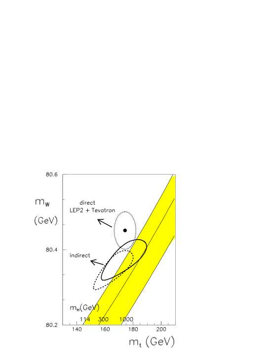
Figure 30: Direct and indirect determinations of $m_{\mathrm{t}}$ and $m_{\mathrm{W}}$. The contours shown are for a confidence level of 70$\%$. The central value of the direct measurements is shown as a solid point and the contour by a dotted line. The indirect determination which is shown as a solid line is for all high q² electroweak measurements, except the direct measurements of $m_{\mathrm{t}}$ and $m_{\mathrm{W}}$. The results obtained when the NuTeV and APV results are also included in the indirect determination is shown as a dashed line.

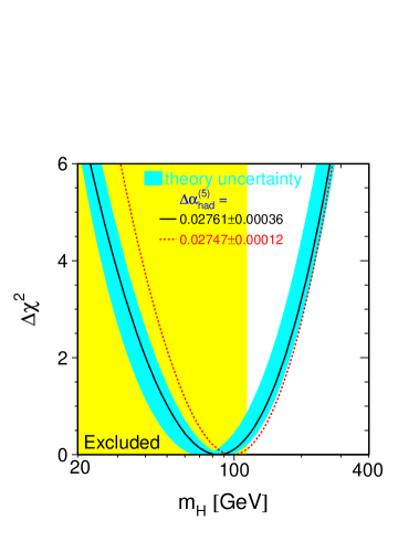
Figure 31: $\Delta\chi^{2}$ as a function of $m_{\mathrm{H}}$ for the global fit to all electroweak data. The shaded region is excluded by direct searches at LEP. The band shows an estimate of the theoretical uncertainty.

The fits given in tab.18 only include electroweak data corresponding to a scale q${}^{2}\simeq m_{\mathrm{Z}}^{2}$. That is, items 8) and 9) in the list of quantities above, which correspond to a scale much below $m_{\mathrm{Z}}^{2}$, are not included. The fitted parameters from a global fit to all the electroweak data, that is items 1)-9) in the above list, are given in tab.19. The $\chi^{2}$ with respect to the minimum value, as a function of the Higgs mass $m_{\mathrm{H}}$, is shown in fig. 31. The central value for $m_{\mathrm{H}}$ is slightly below the lower limit for direct searches at LEP (114 GeV at the 95$\%$ c.l.). Taking into account the theoretical uncertainty (shown as a band), the one-sided 95$\%$ c.l. is $m_{\mathrm{H}}\leq$ 196 GeV. If the value $\Delta\alpha^{(5)}_{had}$(s) = 0.02747 $\pm$ 0.00012 [73] is used, then the upper limit becomes 199 GeV.

Table 19: Results of the global electroweak fit. The $\chi^{2}$/df is 29/15, a probability of 1.7$\%$. The value for $m_{\mathrm{W}}$ is that derived from the fit.

• quantity	fitted value	error
  $m_{\mathrm{t}}$(GeV)	174.7	4.4
  $\alpha_{s}$	0.118	0.003
  $m_{\mathrm{H}}$(GeV)	85	${}^{+54}_{-34}$
  $m_{\mathrm{W}}$(GeV)	80.394	0.018

The pull values of the fitted quantities are shown in fig. 32. The pull for an observable O_i is defined as (O${}_{i}^{\rm meas}$ - O${}_{i}^{\rm fit}$)/$\sigma_{i}^{\rm meas}$. It can be seen that the largest pulls are 3.00 for the NuTeV result and -2.64 for $A^{0,\,{\rm b}}_{\rm{FB}}$. The rms of the pull values is 1.28. This quantity has a statistical uncertainty of 0.17, and so is reasonably compatible with unity.

Figure 32: Pull distribution for the global electroweak fit.

The 70 and 95$\%$ confidence level contours for the parameters $m_{\mathrm{t}}$ and $m_{\mathrm{H}}$ are shown in fig. 33. It can be seen that there is a strong correlation ($\simeq$ 0.7) between $m_{\mathrm{t}}$ and $m_{\mathrm{H}}$. The importance of using the direct measurement of $m_{\mathrm{t}}$ in improving the constraints on $m_{\mathrm{H}}$ can also be seen.

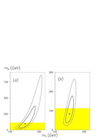
Figure 33: Fitted values of $m_{\mathrm{t}}$ and $m_{\mathrm{H}}$ from a fit to a) all electroweak data except $m_{\mathrm{t}}$ and b) all electroweak data, together with the 70 and 95$\%$ confidence level contours. The shaded region is that excluded by the direct Higgs search at LEP.

Although the global electroweak fits which have been carried out in recent years have always favoured a light Higgs mass, the central fitted values, and the upper limits, have undergone some important changes. For example, at the time of the ICHEP 2000 Conference in Osaka [87], the fitted value was $m_{\mathrm{H}}$ = 60 ${}^{+52}_{-29}$ GeV, with a $\chi^{2}$ probability of 14$\%$. The main input changes in the fits since then are the updates on the measurement of $m_{\mathrm{W}}$, the heavy flavour data, the NuTeV NC/CC ratio, the inclusion of $Q_{\rm W}({\rm Cs})$ and the new value of $\alpha(m_{\mathrm{Z}})$. The effect of the inclusion of each of these separately with respect to the Osaka data is as follows. The updated $m_{\mathrm{W}}$ result alone changes the Osaka $m_{\mathrm{H}}$ value by -6 GeV, while the new heavy flavour data change it by +3 GeV. The inclusion of the new NuTeV NC/CC ratio changes the Osaka $m_{\mathrm{H}}$ value by +3 GeV (but the $\chi^{2}$ increases significantly), whereas the inclusion of $Q_{\rm W}({\rm Cs})$ increases $m_{\mathrm{H}}$ by +2 GeV. However, the largest effect comes from the new $\alpha(m_{\mathrm{Z}})$, which with the Osaka data gives $m_{\mathrm{H}}$ = 88 GeV, i.e. a change of +28 GeV. Thus the overall change of +25 GeV with respect to the Osaka input data comes largely from $\alpha(m_{\mathrm{Z}})$. Note that the correlation between $\alpha(m_{\mathrm{Z}})$ and $m_{\mathrm{H}}$ is about -0.5, so an increase in the value of $\alpha(m_{\mathrm{Z}})$ used leads to a decrease in the fitted $m_{\mathrm{H}}$ value.

As an indication of the importance of the external constraint on $\alpha(m_{\mathrm{Z}})$, a fit to all electroweak data, but without the $\alpha(m_{\mathrm{Z}})$ constraint, gives $m_{\mathrm{H}}$ = 25 ${}^{+39}_{-11}$ GeV. $\alpha(m_{\mathrm{Z}})$ is strongly correlated with $m_{\mathrm{t}}$ and $m_{\mathrm{H}}$, with correlation coefficients of 0.52 and -0.80 respectively.

The various electroweak quantities have different sensitivities to $m_{\mathrm{H}}$. This can be seen in fig.34, where the results from the seven most sensitive individual measurements, M_i, are displayed. In each of these fits only the measurement in question is used and the values $m_{\mathrm{Z}}$ = 91.1875 GeV, $m_{\mathrm{t}}$ = 174.3 GeV, $\alpha_{\rm{s}}{\rm(m_{\mathrm{Z}})}$ = 0.118 and $\Delta\alpha^{(5)}_{had}(m_{\mathrm{Z}})$ = 0.02761 are imposed. If these quantities were allowed to vary in the fit then their correlations with $m_{\mathrm{H}}$ would be different for each M_i. Thus fig.34 displays only part of the influence of the observables M_i in the overall fit. It is of interest to quantify which measured quantities are currently the most sensitive to $m_{\mathrm{H}}$. To see this the measured quantities are set to the SM values, corresponding to $m_{\mathrm{H}}$ = 300 GeV, and the above single measurement fits repeated. The sensitivities, in decreasing order of sensitivity, are $m_{\mathrm{W}}$ (0.19), $A_{\rm{LR}}$ (0.20), $A^{0,\,{\rm b}}_{\rm{FB}}$ (0.24), $\Gamma_{\mathrm{Z}}$ (0.27), $\cal P_{\tau}$ (0.33), $A^{0,\,\ell}_{\rm{FB}}$ (0.45) and $A^{0,\,{\rm c}}_{\rm{FB}}$ (0.65), where the quantities in parentheses are the fit errors on log₁₀($m_{\mathrm{H}}$).

What conclusions can be drawn about $m_{\mathrm{H}}$ from the above results ? There are two, or more, points of view. Firstly, one can note that the overall $\chi^{2}$ of 29/15 df has a probability of 1.7$\%$. Although this is somewhat on the low side, we expect some statistical fluctuations, even if all the measurements are reliable and taken at face value.

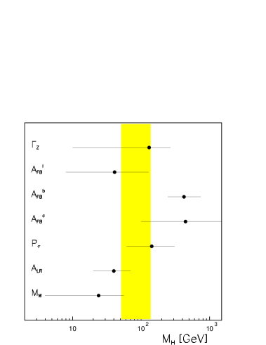
Figure 34: Sensitivity of individual electroweak measurements to the Higgs mass, $m_{\mathrm{H}}$. The error bars shown correspond to one standard deviation. The one standard deviation results of the fit to all the data is shown as a vertical band.

Table 20: Sensitivity of fitted $m_{\mathrm{H}}$ value and upper limit to input data. The NuTeV measurement is not included in these fits.

• fit	$m_{\mathrm{H}}$ GeV	95$\%$ c.l. (GeV)
  standard	81${}^{+49}_{-32}$	174
  if exclude ALR	108${}^{+66}_{-43}$	233
  if exclude $A^{0,\,{\rm b}}_{\rm{FB}}$ and $A^{0,\,{\rm c}}_{\rm{FB}}$	43${}^{+32}_{-18}$	106
  if exclude ALR,$A^{0,\,{\rm b}}_{\rm{FB}}$ and $A^{0,\,{\rm c}}_{\rm{FB}}$	48${}^{+44}_{-23}$	135
  if scale errors	75${}^{+58}_{-35}$	189

An alternative approach is to conclude that the large overall $\chi^{2}$ is either indicating a breakdown of the SM or that one, or more, measurements contributing to the $\chi^{2}$ are, at some level, incorrect.

The largest contribution to the overall $\chi^{2}$ (9 out of 29) comes from the NuTeV NC/CC ratio. If this measurement is removed from the fit the $\chi^{2}$ reduces to 20 (probability of 14$\%$) and the fitted value of $m_{\mathrm{H}}$ is not significantly changed: it is reduced by about 3 GeV. The NuTeV measurement is of great interest, in that it might be an indication of physics beyond the Standard Model. However, the present accuracy, measured in terms of the equivalent uncertainty on value of $m_{\mathrm{W}}$, is such that the inclusion of the result does not significantly change the extracted $m_{\mathrm{H}}$ value, but it does increase substantially the $\chi^{2}$. To investigate the effects of the other measurements, the NuTeV result is omitted in the following considerations.

For the remaining measurements it is mainly the quantities most sensitive to $m_{\mathrm{H}}$ which give the largest contributions to $\chi^{2}$. Namely, $A^{0,\,{\rm b}}_{\rm{FB}}$, $A^{0,\,{\rm c}}_{\rm{FB}}$, $A_{\rm{LR}}$, $m_{\mathrm{W}}$, $A^{0,\,\ell}_{\rm{FB}}$, $\Gamma_{\mathrm{Z}}$ and $\cal P_{\tau}$ contribute 15 to total $\chi^{2}$ of 20, so maybe one should scale these errors by their $\sqrt{\chi^{2}/(df-1))}$ = 1.6 ? Tab. 20 gives the results for the central values and 95$\%$ c.l. upper limits, without consideration of the theoretical uncertainty, for a series of fits. It can be seen that the 95$\%$ c.l. upper limit increases to 233 GeV if the $A_{\rm{LR}}$ measurement is excluded from the fit, but decreases to 106 GeV if $A^{0,\,{\rm b}}_{\rm{FB}}$ and $A^{0,\,{\rm c}}_{\rm{FB}}$ are both excluded. Excluding both $A_{\rm{LR}}$ and the heavy flavour asymmetries $A^{0,\,{\rm b}}_{\rm{FB}}$ and $A^{0,\,{\rm c}}_{\rm{FB}}$ still favours a light Higgs. If the errors of the Higgs sensitive quantities are scaled, as discussed above, then the central value does not change much, but the 95$\%$ c.l. upper limit increases to 189 GeV.

7.3 Direct Higgs search and limits and electroweak fits

In the above discussion neither the lower limit on the direct search for the SM Higgs boson at LEP 2, nor the possible observation of a signal, are taken into account in the electroweak fits. A signal, with a mass of about 115 GeV and compatible with being from the SM Higgs boson, has been found at LEP, with a statistical significance of about 2 standard deviations [3].

In the experimental analysis, the main channel searched for is $\mathrm{e}^{+}\mathrm{e}^{-}\rightarrow$ ZH, followed by the decay H $\rightarrow{\mathrm{b}\overline{\mathrm{b}}}$. This is a threshold process, so the searches for this Z${\mathrm{b}\overline{\mathrm{b}}}$ topology in the highest cms energy runs at LEP 2 ($\sqrt{s}$ up to 209 GeV) were the most important. In the experimental analysis events are classified in terms of the mass $m_{\mathrm{H}}$ of a potential Higss boson and a variable ${\cal G}$ quantifying the Higgs-like nature of the event. This likelihood variable ${\cal G}$ is constructed to be large for a Higgs-like topology and small for a background topology. A likelihood ratio ${\cal L}_{s+b}$/${\cal L}_{b}$ is constructed, as a function of $m_{\mathrm{H}}$, where b is the hypothesis of background only, and s+b that for a Higgs signal plus background. This test statistic amounts essentially to the difference in the $\chi^{2}$ between the two hypotheses, and shows a possible Higgs signal at a mass around 115 GeV [3].

In the analysis the probablility is calculated, as a function of $m_{\mathrm{H}}$, that the background could fluctuate to the level seen in the data, and whether the excess is compatible with the expected production rate of the SM Higgs boson. This latter point is well defined, since the production rate is known if $m_{\mathrm{H}}$ is specified. Note however that, in addition to the possible signal at 115 GeV, there are other signals of smaller significance. Furthermore, nothing can be said about the region beyond the kinematic range of LEP. Indeed, further Higgs bosons could exist at higher masses, as expected in SUSY models. In this case the SM would be shown to be invalid.

In electroweak fits, it is assumed that there is just one Higgs boson of unknown mass. The Higgs mass which gives the best fit to all the data is found and, provided the overall probablility that the SM fits the ensemble of electroweak data is satisfactory, the value or limits found are the best (indirect) estimates of $m_{\mathrm{H}}$, within the context of the SM. Thus the statistical question addressed in the electroweak fits is rather different to that in the direct search, and so the information is difficult to combine. However, it should be noted that the electroweak fits are certainly compatible with a Higgs of mass 115 GeV.

The lower limit on $m_{\mathrm{H}}$ from the direct search at LEP 2 is about 114 GeV, at the 95$\%$ confidence level. Since the production cross-section for the Higgs boson falls off rapidly with increasing Higgs mass, the limit for lower Higgs masses is much more stringent. This lower limit can be represented essentially as a ‘brick wall’ in the $\chi^{2}$ of the electroweak fit, in that we know that the SM Higgs cannot be significantly below the lower limit, or else it would have been observed.

The non observation of the SM Higgs can be incorporated into the electroweak fits, provided additional assumptions are made. It is first assumed that the prior probability for the Higgs boson is uniform as a function of log($m_{\mathrm{H}}$). The $\chi^{2}$ probabilities for the electroweak fits to all data are then computed, as a function of $m_{\mathrm{H}}$, between some very low mass value (in practice 3 GeV is used here) and 1000 GeV, where the theory breaks down. The differential or relative probablity distribution, as a function of log($m_{\mathrm{H}}$), is then constructed, such that the overall probablity that the Higgs is in this mass range is unity. This is because, in the absence of further information, the SM Higgs should exist in this range. The experimental lower limit is taken into account by computing the probability again, this time from a lower limit of 114 GeV up to 1000 GeV. This probability is then normalised to unity, as we are assuming now that the SM Higgs is in this mass range. The distributions of the probabilities obtained, with and without the use of the lower limit, are shown in fig.35. From the cumulative probability distribution a 95$\%$ confidence level upper limit can be extracted. This is about 215 GeV for the case where no lower direct limit is imposed, and rises to about 275 GeV when the direct limit is imposed. This increase in the limit is just a consequence of restributing the unit probability into a more restricted area.

In summary, from the considerations in this and previous sections, the best estimate for the Higgs mass is that it is relatively light. However, the data are not fully compatible, so some caution should be made in drawing conclusions.

Figure 35: Relative probabilty (a) and cumulative probabilty (b), as a function of log₁₀($m_{\mathrm{H}}$), for the cases where no lower limit is imposed (solid circles) and where a lower direct limit of 114 GeV is imposed. This limit is shown as a dashed line.

7.4 Further considerations of the NuTeV result

As discussed in section 6.3, the main discrepancy from the NuTeV data with respect to the SM is in the value of g${}_{L}^{2}$, which is about 1$\%$ below the SM prediction. A recent review of both the theoretical corrections needed for the measurement, and for possible interpretations in terms of physics beyond the SM, can be found in  [88]. The NuTeV analysis assumes that $s=\bar{s}$, for the strange-sea. It is suggested in  [88] that if this equality is violated, such that $s-\bar{s}\simeq$ 0.002, as obtained from neutrino dimuon data, then a good fraction of the anomaly can be explained. However, NuTeV dimuon data give $s-\bar{s}\simeq$ -0.0027 $\pm$ 0.0013. That is, the measured NuTeV asymmetry has the opposite sign, and using this value would increase the significance of the anomaly.

It is interesting to note that the NuTeV data, when interpreted in terms of a deviation of the neutrino NC rate, gives $\rho^{2}$ = 0.9884 $\pm$ 0.0042 [89]. That is, the $\nu$ couplings are (1.16 $\pm$ 0.42)$\%$ less than their SM values. From the results given in section 3.4, it can be computed that the ratio of the invisible width of the Z-boson to the SM value (i.e. for N_ν = 3) is 0.9947 $\pm$ 0.0028, which is (0.53 $\pm$ 0.28)$\%$ less than the SM value. It worth pointing out that the energy scales probed are very different; with q${}^{2}\simeq$ -20 GeV² (t-channel) for the neutrino beam, and q${}^{2}\simeq$ 8300 GeV² (s-channel) at LEP. The current precision of the data is not sufficient to draw any firm conclusion on a possible violation of the SM for the neutrino NC couplings.

Various possibilities in terms of physics beyond the SM, which might explain the NuTeV anomaly (if it is taken to be real) are discussed in  [88]. In general it is found that models which preserve a fair degree of symmetry have difficulty in explaining the results. SUSY models, for example, give effects which are too small in magnitude and of the wrong sign. Only models in which the couplings are much more ad hoc can be tuned to fit the data, but these tend to have a large number of parameters.

7.5 Quasi model-independent variables

The information content of all of the precision electroweak quantities can, to a very good approximation, be described by four quasi model-independent quantities $\epsilon_{1}$,$\epsilon_{2}$,$\epsilon_{3}$ and $\epsilon_{b}$ [90], plus $\alpha_{\rm{s}}{\rm(m_{\mathrm{Z}})}$.

The $\epsilon$’s are defined as follows:

$$\epsilon_{1} = \Delta\rho$$ (71)

$$\epsilon_{2} = \rm{c_{0}^{2}}\Delta\rho+\frac{\rm{s_{0}^{2}}\Delta{r}_{\mathrm{w}}}{(\rm{c_{0}^{2}}-\rm{s_{0}^{2}})}-2\rm{s_{0}^{2}}\Delta\kappa$$ (72)

$$\epsilon_{3} = \rm{c_{0}^{2}}\Delta\rho+(\rm{c_{0}^{2}}-\rm{s_{0}^{2}})\Delta\kappa$$ (73)

where the axial-vector and vector ${\mathrm{Z}}$-lepton couplings are (see eqn. 26)

$$a_{\ell}=-\frac{1}{2}(1+\Delta\rho/2)$$ (74)

and

$$v_{\ell}/a_{\ell}=1-4\sin^{2}\!\theta_{\rm{eff}}^{\rm{lept}}=1-4(1+\Delta\kappa)\rm{s_{0}^{2}}\ \ ,$$ (75)

with

$$\rm{s_{0}^{2}}\rm{c_{0}^{2}}=\frac{\pi\alpha(m_{\mathrm{Z}})}{\sqrt{2}G_{\mathrm{F}}m_{\mathrm{Z}}^{2}}.$$ (76)

Numerically, $\rm{s_{0}^{2}}$ = 0.23118. The quantity $\Delta{r}_{\mathrm{w}}$ is given by $m_{\mathrm{W}}$

$$(1-\frac{\rm{m_{W}^{2}}}{{\rm{m_{Z}^{2}}}})\frac{\rm{m_{W}^{2}}}{{\rm{m_{Z}^{2}}}}=\frac{\pi\alpha(m_{\mathrm{Z}})}{\sqrt{2}G_{\mathrm{F}}{\rm{m_{Z}^{2}}}(1-\Delta{r}_{\mathrm{w}})}.$$ (77)

Inserting the value of $\rm{s_{0}^{2}}$, the expression for $\epsilon_{3}$ becomes

$$\epsilon_{3}=0.77\Delta\rho+0.54\Delta\kappa\ \ .$$ (78)

In this approach it is assumed that new physics, beyond the SM, enters through gauge-boson propagator (vacuum polarisation) functions and/or vertex corrections to the $\mbox{${\mathrm{Z}}$}\ell^{+}\ell^{-}$ vertex, assuming lepton universality. The effects arising through propagator contributions are often called oblique electroweak corrections.

Note that the measurements of the total or partial ${\mathrm{Z}}$ widths, which constrain $\Delta\rho$, contribute to both $\epsilon_{1}$,$\epsilon_{2}$ and $\epsilon_{3}$, whereas measurements of $\sin^{2}\!\theta_{eff}$, from forward-backward or other asymmetry measurements, contribute only to $\epsilon_{2}$ and $\epsilon_{3}$. The direct measurement of the W mass determines $\Delta{r}_{\mathrm{w}}$, and this only enters in the variable $\epsilon_{2}$.

Data on the $\mbox{${\mathrm{Z}}$}q\bar{q}$ vertices can also introduced if it is further assumed that all additional deviations from the SM are contained in the vacuum polarisation functions and/or the $\mbox{${\mathrm{Z}}$}{\rm{b}\bar{\rm{b}}}$ vertex. Further, $\alpha_{\rm{s}}{\rm(m_{\mathrm{Z}})}$ must also be introduced to describe the QCD corrections. A new parameter $\epsilon_{b}$ is needed to describe the $\mbox{${\mathrm{Z}}$}{\rm{b}\bar{\rm{b}}}$ vertex and is defined such that

$$a_{\rm{b}}=a_{\ell}(1+\epsilon_{b})$$ (79)

and

$$\frac{v_{\rm{b}}}{a_{\rm{b}}}=\frac{1-\frac{4}{3}\sin^{2}\!\theta_{\rm{eff}}^{\rm{lept}}+\epsilon_{b}}{1+\epsilon_{b}}.$$ (80)

The determination of $\epsilon_{b}$ comes essentially from the measurement of $R_{\mathrm{b}}$. As noted previously, the forward-backward asymmetries for heavy-quarks depend mainly on $\cal A_{\rm e}$. For the other quarks, small corrections are made in order to obtain $\Delta\rho$ and $\Delta\kappa$ from the extracted values of the quark vector and axial-vector couplings. These corrections are computed in the SM. Corrections are made for QCD effects where necessary, using the ZFITTER package. With these additions, all the LEP and SLD measurements can be included in the fits.

In the SM, the main dependence on $m_{\mathrm{t}}$ is either quadratic or logarithmic, whereas the dependence on $m_{\mathrm{H}}$ is only logarithmic. The parameter $\epsilon_{1}$ depends on $m_{\mathrm{t}}^{2}$ and ln($m_{\mathrm{H}}$), $\epsilon_{2}$ depends on ln($m_{\mathrm{t}}$) , $\epsilon_{3}$ depends on ln($m_{\mathrm{H}}$) and ln($m_{\mathrm{t}}$) and $\epsilon_{b}$ depends on $m_{\mathrm{t}}^{2}$. The SM contributions to the $\mbox{${\mathrm{Z}}$}{\rm{b}\bar{\rm{b}}}$ vertex come from t-W-b loops.

Of course, the usefulness of these variables, or the closely related S,T and U variables [91], is in studying physics beyond the SM. The aim is thus to reduce the errors on the $\epsilon$’s to be as small as possible, so as to be as sensitive as possible to such physics.

The result of a fit to the electroweak data is given in table 21 . The contour plots for the 70% confidence levels for $\epsilon_{1}$, $\epsilon_{2}$ and $\epsilon_{3}$ are also shown in fig. 36. The direct top-quark mass measurement and the NuTeV result are not included, the latter because the result is expressed as a function of $m_{\mathrm{t}}$ and $m_{\mathrm{H}}$. The value of $\alpha(m_{\mathrm{Z}})$ is constrained according to eqn.(55). The value of $\alpha_{\rm{s}}{\rm(m_{\mathrm{Z}})}$ is fitted from the data. If the constraint $\alpha_{\rm{s}}{\rm(m_{\mathrm{Z}})}$ = 0.118 $\pm$ 0.002 is imposed, then the central values of the $\epsilon$ variables are shifted by only a small amount. The results are, as expected, compatible with the SM expectations at the values of $m_{\mathrm{t}}$ and $m_{\mathrm{H}}$ discussed in previous sections (see fig. 36). From table 21 it can be seen that the value of $\epsilon_{b}$ is strongly correlated to that of $\alpha_{\rm{s}}{\rm(m_{\mathrm{Z}})}$. In the SM, $\epsilon_{b}$ = -5.8 10^-3 for $m_{\mathrm{t}}$ = 175 GeV, and is essentially independent of $m_{\mathrm{H}}$.

The variable $\epsilon_{1}$ is sensitive to new physics which violates the custodial weak isospin symmetry, whereas $\epsilon_{3}$ is an isospin symmetric observable. The $\epsilon$ (or S,T,U) variables have been used to place severe constraints on some technicolour theories. In these theories (see e.g. [94]) an alternative approach to symmetry breaking is advocated, in which the symmetry breaking arises from strongly interacting technicolour effects. Technicolour is analoguos to QCD, but with an expected characteristic scale of $\Lambda_{TC}\simeq$ 500 GeV, compared to the QCD scale $\Lambda\simeq$ 200 MeV. There should also be a spectrum of techniparticles (techni$\pi$, techni$\rho$ etc.), none of which have so far been observed. The most reliable predictions are for the variable $\epsilon_{3}$. For the simplest cases [91], the deviation from the SM value of $\epsilon_{3}$ is given in terms of the number of technicolours ${\rm{N_{TC}}}$ as

$$\Delta\epsilon_{3}\simeq\left\{\begin{array}[]{ll}0.0035+0.0009({\rm{N_{TC}}}-4)&\\ 0.013+0.003\ ({\rm{N_{TC}}}-4),&\\ \end{array}\right.$$ (83)

where the first line is for a doublet of ${\rm{N_{TF}}}$ = 2 technifermions, and the second line for a full technigeneration (${\rm{N_{TF}}}$ = 8). An alternative formulation [91] gives $\Delta\epsilon_{3}\simeq 0.0024({\rm{N_{TF}}}/2)({\rm{N_{TC}}}/3)$, giving values close to those of eqn.(83).

The experimental limit on $\Delta\epsilon_{3}=\epsilon_{3}$(meas) - $\epsilon_{3}$(SM) is $\Delta\epsilon_{3}\leq$ 1.5 10^-3, at the 95$\%$ c.l. Thus, within the context of this technicolour model, a full technigeneration can be excluded, and a single doublet of technifermions is almost excluded. However, in developments of the technicolour ideas in walking technicolour [95], and other variants, these limits can be evaded, since $\Delta\epsilon_{3}$ can be smaller or even negative. Note that, in general, QCD-like models have difficulties in preventing flavour-changing neutral-currents or in giving too fast a rate for proton decay.

An alternative scenario for new physics is the existence of a fourth generation of fermions, which are heavy on the scale of $m_{\mathrm{Z}}$. These would contribute through $\mathrm{f}\bar{\mathrm{f}}$ loop corrections to the propagators. A complete heavy degenerate fourth generation would contribute $\Delta\epsilon_{3}$ = 0.0017, and so is at the limit of exclusion at the 95$\%$ c.l.

The effect of SUSY depends on the mass spectrum of the SUSY particles. In the ‘heavy’ limit, where all the s-particles are rather massive, then the MSSM predictions tend to reproduce the SM results corresponding to a light Higgs in the region $m_{\mathrm{H}}\simeq$ 100 GeV (see [96]). This scenario is, of course, compatible with the electroweak data.

Table 21: Results of the fit to the $\epsilon$ variables to all electroweak data, with the exception of the direct measurement of $m_{\mathrm{t}}$. The correlation matrix is also given. The $\chi^{2}$ for the fit is 16/10 df, a probability of 11%.

parameter	fitted value	$\epsilon_{1}$	$\epsilon_{2}$	$\epsilon_{3}$	$\epsilon_{b}$	$\alpha_{\rm{s}}{\rm(m_{\mathrm{Z}})}$
$\epsilon_{1}$	$(5.7\pm 1.0)10^{-3}$	1.00	0.62	0.86	0.00	-0.37
$\epsilon_{2}$	$(-9.4\pm 1.2)10^{-3}$		1.00	0.40	0.00	-0.26
$\epsilon_{3}$	$(5.5\pm 1.0)10^{-3}$			1.00	0.02	-0.27
$\epsilon_{b}$	$(-4.2\pm 1.6)10^{-3}$				1.00	-0.64
$\alpha_{\rm{s}}{\rm(m_{\mathrm{Z}})}$	$0.115\pm 0.004$					1.00

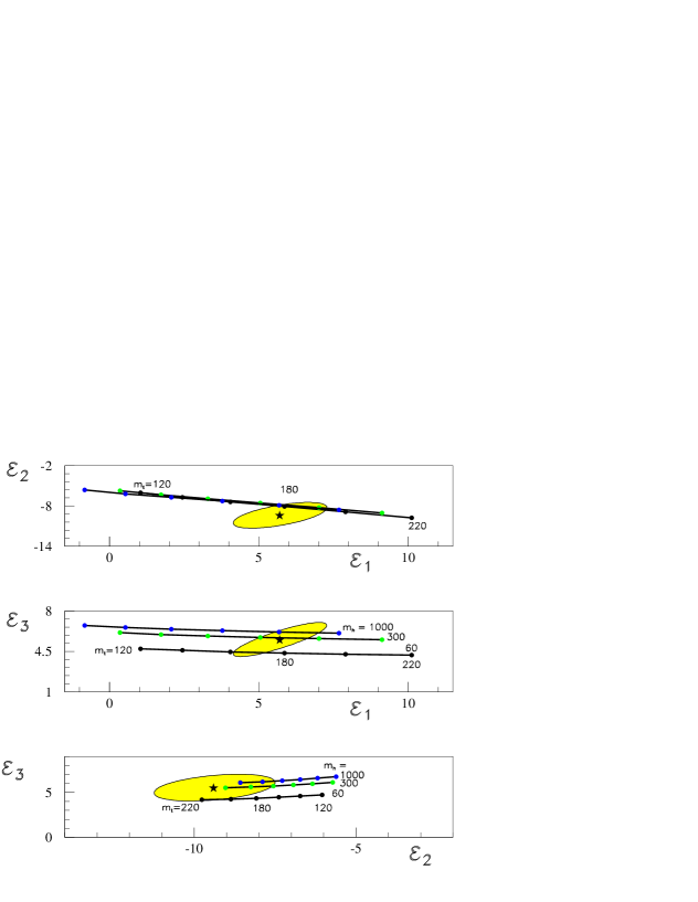
Figure 36: Results of a fit to $\epsilon_{1}$, $\epsilon_{2}$ and $\epsilon_{3}$, in units of 10^-3, showing the 70% confidence level contours and the expectations in the SM, for different values of $m_{\mathrm{t}}$ and $m_{\mathrm{H}}$. For $\epsilon_{1}$ versus $\epsilon_{2}$ there is little sensitivity to $m_{\mathrm{H}}$.

8 Future prospects

Table 22: Effect of expected improved precision on $m_{\mathrm{H}}$.

• fit	$m_{\mathrm{H}}$ GeV	$\chi^{2}$/df
  now: $\delta m_{\mathrm{t}}=\pm$ 5.1 GeV, $\delta m_{\mathrm{W}}=\pm$ 33 MeV	85${}^{+54}_{-34}$	29 / 15
  if $\delta m_{\mathrm{t}}=\pm$ 2.0 GeV, $\delta m_{\mathrm{W}}=\pm$ 33 MeV	83${}^{+38}_{-28}$	29 / 15
  if $\delta m_{\mathrm{t}}=\pm$ 5.1 GeV, $\delta m_{\mathrm{W}}=\pm$ 15 MeV	67${}^{+40}_{-27}$	34 / 15
  if $\delta m_{\mathrm{t}}=\pm$ 2.0 GeV, $\delta m_{\mathrm{W}}=\pm$ 15 MeV	50${}^{+21}_{-16}$	35 / 15
  if $\delta m_{\mathrm{t}}=\pm$ 1.0 GeV, $\delta m_{\mathrm{W}}=\pm$ 10 MeV	35${}^{+12}_{-10}$	38 / 15

If the Higgs mass were $m_{\mathrm{H}}$ = 115 $\pm$ 1 GeV, as the direct search at LEP 2 might indicate, then if this constraint is introduced into the SM fit using the present measurements, the top-quark mass increases by 2.0 GeV, due to the correlation with $m_{\mathrm{H}}$. The error is reduced from $\delta m_{\mathrm{t}}=\pm$ 4.4 to $\pm$ 3.1 GeV. The $\chi^{2}$ probability increases slightly to 2.2$\%$, and the other quantities are largely unchanged, since the standard fit is compatible with this Higgs mass.

Some improvements are expected, in the relatively near future, on the precision of the W boson and top quark masses. For $m_{\mathrm{W}}$, the final LEP value is still awaited and Run 2, at the Tevatron, should produce a much improved precision compared to Run 1. The same holds for the top quark mass. It is difficult to make a precise estimate of the improvements, but to give an indication of what the impact would be, $\delta m_{\mathrm{t}}=\pm$ 2.0 GeV and $\delta m_{\mathrm{W}}=\pm$ 15 MeV are taken. The effect of these on the global electroweak fit is given in tab.22, where it is assumed that the present central values remain unchanged. It can be seen that improved precision in the measurements of both $m_{\mathrm{W}}$ and $m_{\mathrm{t}}$ is needed. If this were achieved, and if the central values remain unchanged, then the 95$\%$ c.l. upper limit for $m_{\mathrm{H}}$ would be 87 GeV, plus the theory uncertainty. This would be incompatible with the direct search limits, and thus would indicate a breakdown of the SM. If the limits given in the last line of tab.22 could be achieved, namely $\delta m_{\mathrm{t}}=\pm$ 1.0 GeV and $\delta m_{\mathrm{W}}=\pm$ 10 MeV, this would give a very precise central value for $m_{\mathrm{H}}$, and the 95$\%$ c.l. upper limit would reduce to 56 GeV.

9 Summary

Most of the LEP 1 data, apart from some of the heavy flavour data, are now finalised and published. For the ${\mathrm{Z}}$-fermion couplings at a scale q${}^{2}\simeq m_{\mathrm{Z}}^{2}$, those of the b-quark, and to a lesser extent those of the $\tau$-lepton, are the least consistent with SM expectations. More precise data are needed to see if there is indeed an inconsistency for the third fermion generation.

The measurements from the NuTeV experiment might also indicate an inconsistency in the SM. It is thus important that this situation is resolved by improved experiments.

The Higgs mass appears to be relatively light, but some of the data are rather inconsistent. More work on $\alpha(m_{\mathrm{Z}})$ is needed, as this quantity has a strong influence on the extracted $m_{\mathrm{H}}$ value. The precision on both $m_{\mathrm{W}}$ and $m_{\mathrm{t}}$ needs to be improved at the Tevatron in order to significantly improve the accuracy on the Higgs mass. This is important, particularly if the central values remain essentially unchanged. In this case, there would be clear incompatibilities in the Standard Model.

References

References

- [1] P.B. Renton, (1990) Electroweak Interactions (Cambridge University Press).
- [2] Particle Data Group, D.E. Groom et al, (2000) Eur. Phys.J C15 and http://pdg.lbl.gov.
- [3] F. Gianotti, Searches for New Particles at Colliders, EPS Conference on High Energy Physics, Budapest, Hungary, July 2001 and CERN-EP/2001-055.
- [4] K. Kodama et al, (2001) Phys. Lett. B 504 218; hep-ex/0012035.
- [5] D. Schaile, (1994), proceedings of the XXVII’th ICHEP, Glasgow, Scotland, July 1994.
- [6] V.A. Novikov et al (1999) Rep. Prog. Phys. 62 1275.
-
[7]
D. Bardin and G. Passarino, Upgrading of Precision
Calculations for Electroweak Observables, hep-ph/9803425;
D. Bardin and G. Passarino, (1999) The Standard Model in the making, (Clarendon Press);
D. Bardin, G. Passarino and M. Grünewald, Precision Calculation Project Report, hep-ph/9902452 . - [8] A Combination of Preliminary Electroweak Measurements and Constraints on the Standard Model, The LEP Collaborations ALEPH, DELPHI, L3, OPAL and the LEP Electroweak Working Group; CERN-EP/2001-098, 2001 and hep-ex/0112021.
- [9] D. Bardin et al, (1988) Phys. Lett. B206 539.
- [10] A. Olshevski, P. Ratoff and P.B. Renton, (1993) Z. Phys. C 60 643.
- [11] R. Assmann et al, (1995) Z.Phys. C 66 567.
- [12] R. Assmann et al, (1999) Eur. Phys. J. C 6 187.
- [13] ALEPH Collaboration, R. Barate et al, (2000) Eur. Phys. J. C 14 1.
- [14] DELPHI Collaboration, P. Abreu et al, (2000) Eur. Phys. J. C 16 371.
- [15] L3 Collaboration, M. Acciarri et al, (2000) Eur. Phys. J. C 16 1.
- [16] OPAL Collaboration, G. Abbiendi et al, (2001) Eur. Phys. J. C 19 587.
- [17] S. Jadach et al, (1995) Phys. Lett. B353 362.
- [18] B.F.L. Ward et al, (1999) Phys. Lett. B 450 262.
- [19] G. Montagna et al, (1999) Phys. Lett. B 459 649.
- [20] W. Beenakker and G. Passarino, (1998) Phys. Lett. B425 199.
- [21] Combination Procedure for the precise determination of Z boson parameters from results of the LEP experiments; (2000), CERN-EP-2000-153; unpublished.
-
[22]
TOPAZ0,
G. Montagna et al, (1993) Nucl. Phys. B401 3;
Comp. Phys. Comm. (1996) 93 120; Comp. Phys. Comm. (1999) 117 278. - [23] ZFITTER, D. Bardin et al , (1989) Z. Phys. C44 493; (1990) Comp. Phys. Comm. 59 303; (1991) Nucl. Phys. B351 1; (1991) Phys. Lett. B255 290; CERN-TH 6443/92 (1992) and DESY report 99-070 (1999); (2001) Comp. Phys. Comm. 133 229.
- [24] MIZA, L. Garrido et al, (1991) Z. Phys. C 49 645; M. Martinez and F. Teubert, (1995) Z. Phys. C 65 267.
- [25] S. Jadach et al, (1992) Phys. Lett. B257 173.
- [26] M. Skrzypek, (1992) Acta Phys. Pol. B23 135.
- [27] G. Montagna et al, (1997) Phys. Lett. B406 243.
- [28] D.R. Yennie et al, (1961) Ann. Phys (NY) 13 379.
- [29] E.A. Kuraev and V.S. Fadin, (1985) Sov. J. Nucl. Phys. 41 466.
- [30] F.A. Berends et al, (1988) Nucl. Phys. B 297 429 and (1988) 304 921 (E).
- [31] B.A. Kniehl et al, (1988) Phys. Lett. B 209 337.
- [32] S. Jadach et al, (1992) Phys. Lett. B 280 129.
- [33] S. Jadach et al, (1999) Phys. Lett. B 456 77.
- [34] S. Jadach et al, (1999) Phys. Lett. B 465 254.
- [35] D. Bardin, EPS-HEP99, Tampere, Finland, 15-21 July 1999.
- [36] K. Abe et al, SLD Collaboration, Phys. Rev. Lett. (2000) 84 5945.
- [37] K Abe et al, SLD Collaboration, (2001) Phys. Rev. Lett. 86 1162.
- [38] K. Winter, Neutrino Properties and Interactions, proceedings of the 17th International Symposium on Lepton-Photon Interactions, August 10-15 1995, Beijing, China; p569, World Scientific, Singapore (1996).
- [39] The top averaging group, L. Demortier et al, for the CDF and D0 Collaborations, FERMILAB-TM-2084 (1999).
- [40] P.B. Renton, Review of Experimental Results on Precision Tests of Electroweak Theories, proceedings of the 17th International Symposium on Lepton-Photon Interactions, August 10-15 1995, Beijing, China; p35, World Scientific, Singapore (1996).
- [41] S. Catani and M. Seymour, (1999) JHEP 9907 23; hep-ph/9905424.
- [42] A Combination of Preliminary Electroweak Measurements and Constraints on the Standard Model, The LEP Collaborations ALEPH, DELPHI, L3, OPAL and the LEP Electroweak Working Group; CERN-EP/-2000-016, (2000); unpublished.
- [43] SLD Collaboration, N.De Groot, talk presented at the XXXVIth Rencontre de Moriond, Les Arcs, March 2001; hep-ex/0105058.
- [44] The LEP Experiments, ALEPH, DELPHI, L3 and OPAL, (1996) Nucl. Inst. Meth. A378, 101.
- [45] P.B. Renton, (1999) Eur. Phys. J. C 8 585.
- [46] OPAL Collaboration, PN469, paper submitted to the EPS Conference on High Energy Physics, Budapest, Hungary, July 2001.
- [47] S.D. Drell and T.M. Yan (1970) Phys. Rev. Lett. 25 316.
- [48] T. Affolder et al, CDF Collaboration, (2001) Phys. Rev. Lett. 87 131802.
- [49] J. Rosner, M. Worah, T. Takeuchi, Phys. Rev. D49 1363 (1994).
- [50] N. Cabibbo, (1963) Phys. Rev. Lett. 10 531.
- [51] M. Kobayashi and T. Maskawa, (1973) Prog. Th. Phys. 49 652.
- [52] V. Versi, Electroweak Interactions and Unified Theories, XXXVIth Rencontres de Moriond, March 2001.
- [53] M. Lancaster, proceedings of the 19th International Symposium on Lepton-Photon Interactions, LP99, August 9-14 1999, Stanford CA, USA; p333, World Scientific, Singapore (1999).
- [54] J. Alitti et al, UA2 Collaboration, (1992) Phys. Lett. B 276 354.
- [55] T. Affolder et al, CDF Collaboration, (2001) Phys. ReV. D 64 052001.
- [56] S. Abachi et al, D0 Collaboration, (2000) Phys. Rev. Lett. 84 222.
- [57] R. Barate et al, ALEPH Collaboration, (1997) Phys. Lett. B 401 347; (2000) Eur. Phys. J. C 17 241.
- [58] P. Abreu et al, DELPHI Collaboration, (1997) Phys. Lett. B 397 158; (1999) Phys. Lett. B 462 410.
- [59] M. Acciarri et al, L3 Collaboration, (1997) Phys. Lett. B 398 223; (1999) Phys. Lett. B 454 386.
- [60] K. Ackerstaff et al, OPAL Collaboration, (1996) Phys. Lett. B 389 416; G. Abbiendi et al, (1999) Phys. Lett. B 453 138.
- [61] C. Gerber, New Tevatron Results, EPS Conference on High Energy Physics, Budapest, Hungary, July 2001.
- [62] T. Affolder et al, CDF Collaboration, (2000) Phys. Rev. Lett. 85, 3347.
- [63] YFSWW, S. Jadach et al, (2000) Phys. Rev. D61 113010; hep-ph/0007012; and references therein.
- [64] RACOONWW, A. Denner et al, (2000) Phys. Lett. B475 127; hep-ph/0101257; and references therein.
- [65] S. Eidelman and F. Jegerlehner, (1995) Z.Phys. C67 585.
- [66] H. Burkhardt and B. Pietrzyk, (1995) Phys. Lett. B356 398.
- [67] R. Alemany, M. Davier and A. Hocker, (1998) Eur. Phys. J. C 2 123.
- [68] M. Davier and A. Hocker, (1998) Phys. Lett. B419 419.
- [69] J.H. Kuhn and M. Steinhauser, (1998) Phys. Lett. B437 425.
- [70] J. Erler, (1999) Phys. Rev. D59 054008.
- [71] A.D. Martin, J. Outhwaite and M.G. Ryskin, (2000) Phys. Lett. B492 69.
- [72] H. Burkhardt and B. Pietrzyk, (2001) Phys. Lett. B513 46.
- [73] J.F.d. Troconiz and F.J. Yndurain, hep-ph/0111258 (2001), Proc. of the Budapest 2001 EPS HEP Conference and (2002) Phys.Rev. D65 093002; hep-ph/0107318.
- [74] H.N. Brown et al, Muon (g-2) Collaboration, (2001) Phys.Rev. Lett. 86 2227.
- [75] M. Knecht and A. Nyffeler, (2002) Phys.Rev. D65 073034; M. Knecht et al, (2002) Phys.Rev. Lett. 88 071802; for a review see J. Prades (2001) arXiv:hep-ph/0108192.
- [76] CDF Collaboration, F. Abe et al , (1994) Phys.Rev. Lett. 73 225; (1994) Phys.Rev. D50 2966; (1995) Phys.Rev. Lett. 74 2626.
- [77] D0 Collaboration, S. Abachi et al , (1995) Phys. Rev. Lett. 74 2632.
- [78] CDF Collaboration, F. Abe et al, (1997) Phys.Rev. Lett. 79 1992.
- [79] D0 Collaboration, S. Abbott et al , (1998) Phys.Rev. D58 052001.
- [80] C.S. Wood et al, (1997) Science 275 1759.
- [81] S.C. Bennett and C.E. Wieman, (1999) Phys. Rev. Lett. 82 2484.
- [82] A. Derevianko, (2000) Phys. Rev. Lett. 85 1618.
- [83] M.G. Koslov, S.G. Porsev and I.I. Tupitsyn, (2001) Phys. Rev. Lett. 86 3260.
- [84] V.A. Dzuba, V.V. Flambaum and J.S.M. Ginges, (2001) hep-ph/0111019.
- [85] E.A. Paschos and L. Wolfenstein, (1973) Phys. Rev. D7 91.
- [86] G.P. Zeller et al, NuTeV Collaboration, Phys. Rev. Lett. (2002) 88 091802, and hep-ex/ 0110059.
- [87] A Combination of Preliminary Electroweak Measurements and Constraints on the Standard Model, The LEP Collaborations ALEPH, DELPHI, L3, OPAL and the LEP Electroweak Working Group; CERN-EP/-2001-021, 2001.
- [88] S. Davidson et al, (2001) JHEP 0202 037; hep-ph/0112302.
- [89] K. McFarland, Les Rencontres de Physique de la Vallee d’ Aoste, March 2002.
- [90] G. Altarelli, R. Barbieri and F. Caravaglios, (1993) Nucl. Phys. B405 3.
- [91] M.E. Peskin and T. Takeuchi, (1990) Phys. ReV. Lett. 65 964 and (1991) Phys ReV. D46 381.
- [92] P.B. Renton, (1992) Z. Phys. C 56 355.
- [93] P.B. Renton, (1997) Int. Journ. Mod. Phys. A12 4109.
- [94] E. Farhi and L. Susskind, (1981) Phys Rep. 277.
- [95] R. Sundrum and S.D.H. Hsu, (1993) Nucl. Phys. B391 127.
- [96] R. Barbieri, F. Caravaglios and M. Frigeni, (1992) Phys. Lett B279 169.