The Chiral Phase Transition in Dissipative Dynamics

Abstract

Numerical simulations of the chiral phase transition in the (3+1)dimensional $O(4)$-model are presented. The evolutions of the chiral field follow purely dissipative dynamics, starting from random chirally symmetric initial configurations down to the true vacuum with spontaneously broken symmetry. The model stabilizes topological textures which are formed together with domains of disoriented chiral condensate (DCC) during the roll-down phase. The classically evolving field acts as source for the emission of pions and $\sigma$ mesons. The exponents of power laws for the growth of angular correlations and for emission rates are extracted. Fluctuations in the abundance ratios for neutral and charged pions are compared with those for uncorrelated sources as potential signature for the chiral phase transition after heavy-ion collisions. It is found that the presence of stabilizing textures (baryons and antibaryons) prevents sufficiently rapid growth of DCC-domain size, so observability of anomalous tails in the abundance ratios is unlikely. However, the transient formation of growing DCC domains causes sizable broadening of the distributions as compared to the statistical widths of generic sources.

PACS numbers: 05.45.-a,11.10.Lm,11.30.Rd, 11.27.+d,12.39.Fe,25.75.-q,64.60.Cn,75.40.Mg

Keywords: Chiral Phase Transition, Disoriented Chiral Condensate, Sigma models,

Topological textures, Skyrmions, Bags, Heavy-Ion Collisions

I Introduction

There is general consent that the energy densities achieved in relativistic heavy-ion collision experiments performed or planned at RHIC or LHC should be sufficient to drive hadronic matter through the QCD transition into a new phase with restored chiral symmetry and, probably, deconfined color. A commonly accepted scenario [1] assumes that immediately after (central) collisions most of the baryon number is still concentrated in Lorentz-contracted pancakes receding from the collision point with approximately the speed of light (in beam direction), leaving behind in the c.m. system a rapidly expanding cylindrical or spherical fireball of highly excited ”vacuum”. Although almost void of net baryon number, the energy density initially deposited in this ’fireball’ is sufficient to produce during the subsequent cooling phase a large number of hadronic particles, mostly pions, but also heavier mesons and baryon-antibaryon pairs. If inside the initial hot fireball chiral symmetry indeed has been restored, then during the following relaxation process the relevant order parameter, the chiral condensate, must re-increase to finally approach the nonzero value which characterizes the true vacuum. The time scale for this evolution of the order parameter is set by typical relaxation times $\tau$ of the strongly interacting system (e.g. through dissipation of energy by particle emission) which need not necessarily be closely tied to kinematic time scales $\tau_{c}$ of the collision and expansion time of the fireball. If it is possible to replace during this relaxation process the complex dynamics of the strongly interacting fermionic and bosonic elementary degrees of freedom by effective dynamics for an order-parameter field, then the time scale for changes in the relevant effective potential can be quite distinct from the time scales of dissipative processes which characterize the relaxation of the order parameter towards low-energy configurations in the changing effective potential. So, within that concept we can study evolutions which proceed through sequences of configurations which are far from equilibration. Especially, for $\tau_{c}\ll\tau$, (the so-called ”sudden quench”), the system moves through maximally non-equilibrated sequences.

The standard tool for an effective description of hadronic physics proceeding on energy scales of less than 1 GeV is the chiral $O(4)$ model. The isoscalar quark condensate $\left<\bar{q}q\right>$ (with finite value $\left<\bar{q}q\right>_{0}$ in the true vacuum) is combined with a corresponding isovector condensate $\left<\bar{q}\vec{\tau}q\right>$ to form a four-component ”chiral” field $\Phi$, considered as space-time-dependent order-parameter field, and subjected to an effective action which governs the ”chiral dynamics”. (We do not discuss here the natural extension to the full SU(3) flavor group.) Fluctuations of $\Phi$ describe the pseudoscalar pions and scalar $\sigma$-mesons. In its simplest form, the ”linear $\sigma$-model”, the effective action comprises the kinetic two-gradient term and an appropriate time- or temperature-dependent $\Phi^{4}$ potential. In this form the model has been widely used for investigating features of the chiral phase transition, both in classical dynamics [2], including dissipation and noise [3], and in quantum field theoretical approaches [4].

The generic structure of this model applies to a wide variety of physical systems with spontaneously broken symmetry, such that particular phenomena may be expected to occur irrespective of the nature of the underlying physical degrees of freedom. Depending on the number of field components and spatial dimensions the formation of ordered domains, separated by topological defects or textures characterizes ordering evolutions in all such systems [5]. This analogy has prompted the idea to use pions emitted from differently oriented ordered domains as indicator for the chiral phase transition itself [6]. It is expected that the temporary misalignment of the chiral field in finite spatial domains (as compared to the orientation of $\Phi$ in the true vacuum) leads to anomalous fluctuations in the multiplicities of emitted charged or neutral pions which may provide a signature for the transient existence of disoriented chiral condensate (DCC).

On the other hand, for temperature $T$=0 the interpretation of topologically nontrivial $\Phi$-configurations as baryons [7] (in linear or nonlinear realizations of the $O(4)$-symmetry) has provided surprisingly successful models for baryon structure and dynamics. Their stabilization requires additional terms in a gradient expansion of the effective action. Their form is fixed by chiral symmetry, the magnitude of the few relevant low-energy constants is extracted from experimental information. These higher-order gradient terms incorporate at least partly the influence of vector mesons. Naturally, the well-established Skyrme term is the appropriate and simplest tool for this purpose.

As it is well known that stable textures play a most important role in the ordering evolutions of multi-component fields, it appears essential to allow for their formation and stabilization in the dynamics of evolving field configurations. At the same time this opens up the possibility to describe creation and annihilation of baryonic structures during the evolution of the fireballs. These structures have to be supplied with a definite spatial length scale which is provided by the stabilizing mechanism in the effective action, which prevents them from collapse or indefinite growth. Using all four components of the $O(4)$-field as independent variables implies that in the phase with restored symmetry the absolute value of the condensate can be very small locally, as compared to its true vacuum value. This is different from the nonlinear version of the $O(4)$-model where $\Phi$ is restricted to the 3-sphere $\Phi^{2}=f_{\pi}^{2}$ and symmetry restoration can only occur through spatial averaging over different orientations.

The true vacuum which surrounds the fireball sets the boundary condition for the evolution of the ordering field such that $\mbox{\boldmath$\Phi$}(\mbox{\boldmath$x$},t)$ approaches a fixed vector for $r\to\infty$. In that case, all configurations of the nonlinear model fall into classes distinguished by integer winding numbers $B$. The same is true for configurations $\mbox{\boldmath$\Phi$}(\mbox{\boldmath$x$},t)$ of the linear $O$(4)-model, as long as vanishing field vectors are excluded. While $B$ in the nonlinear model is topologically conserved in time, in the linear version integer jumps in $B$ may occur if at some point in spacetime $\mbox{\boldmath$\Phi$}(\mbox{\boldmath$x$},t)$ moves through $\mbox{\boldmath$\Phi$}=0$. Topologically nontrivial configurations with nonvanishing $\Phi$ embedded in the surrounding vacuum field then are interpreted as baryons with baryon number $B$. In the nonlinear version of the $O$(4)-model these ’baryons’ (with baryon number $B$ and definite size) are topologically stable against unwinding. In the linear $O$(4)-model they represent metastable configurations which occasionally may unwind, especially if chiral symmetry is broken explicitly through a non-vanishing pion mass. As topological arguments do not apply to lattice implementations, $B$-conservation if desired has to be imposed in both cases (linear or nonlinear $O$(4)-model) by an optional additional constraint, which rejects occasional configuration updates that would imply a jump in $B$.

Numerical simulations based on such very specific effective actions which incorporate definite scales will provide answers for physical observables which characterize the specific physical system under consideration. So, it is not so much our aim to look for universal features of a certain class of models, but rather to obtain statements about specific physical situations which hopefully comprise the essentials of a selected class of experiments.

If, during the initial stages of the fireball evolution, color indeed is deconfined, then evidently, the applicability of the $O(4)$-model is restricted to a later phase where the color-degrees of freedom are re-frozen into the colorless order-parameter field $\Phi$. We assume that this local color-confining process does not lead to any preferred local direction of the chiral field. So, assuming that the relaxation of $\Phi$ is driven by effective chiral dynamics, implies that color-confining transition and the restoration of chiral symmetry may be considered separately.

Although dissipative evolution of the order-parameter field is a classical concept, the field fluctuations around the evolving configurations acquire particle properties and must be quantized as emitted radiation. With the classical field acting as a source for the emission of field quanta it is expected that the radiation carries signatures of the source field configuration. This idea underlies the search for DCC effects in the pion yields after heavy-ion collisions. To define the separation of the classically evolving part from the quantum fluctuations we remove all propagating terms (second time-derivatives) from the equations of motion for the classical configuration, i.e. the classical evolution is defined as solution of the purely dissipative Time-Dependent-Ginsburg-Landau (TDGL) equations. As a consequence, the radiation is driven by the instantaneous field velocities, from which the event-by-event fluctuations in abundance ratios may be obtained.

The following discussion represents an extension of previous work dealing with corresponding features in the lower-dimensional (2+1)d $O$(3) model [8]. In contrast to the exploratory nature of the previous investigations we here attempt to define the model as close as possible to the scales which characterize actual hadronic matter and to the physical situation which might prevail after an ion-ion collision. In Chpt.II we formulate the equations of motion and the resulting emission rates. For comparison we present also the corresponding expressions for the abundance ratios for DCC sources and for uncorrelated stochastic sources. The model and the relevant parameters which will be used for the numerical evolutions are specified in Chpt.III. In Chpt.IV the initial and boundary conditions for these evolutions are defined, together with important observables measured during individual evolutions, like net baryon number, baryon plus antibaryon number, equal-time angular correlations as a measure for the size of disoriented domains. Chpt.V presents numerical results, from which typical exponents for growth laws are extracted. These are finally used to draw conclusions about the possibility to observe signatures of the chiral phase transition from charge fluctuations in the pion radiation emitted from the relaxing source.

II Nonequilibrium field dynamics and DCC signals

A The TDGL equations

We consider an effective action for an $O(4)$ vector field $\Phi$

$${\cal S}[\mbox{\boldmath$\Phi$}]=\int\left({\cal T}[\mbox{\boldmath$\Phi$}]-{\cal U}[\mbox{\boldmath$\Phi$}]\right)d^{3}xdt$$ (1)

where the kinetic energy density ${\cal T}[\mbox{\boldmath$\Phi$}]$ comprises all terms containing time-derivatives of $\Phi$. We follow the evolution of field configurations, which at some initial time deviate from the global equilibrium configuration (the ’true vacuum’) within some finite spatial region $V$. The equations of motion $\delta{\cal S}/\delta\mbox{\boldmath$\Phi$}=0$ which govern the classical evolution of the initial non-equilibrium configuration describe both, the approach towards the vacuum configuration in the interior of that spatial region and the propagation of outgoing (distorted) waves into the (initially undisturbed) surrounding vacuum. Although, of course, the classical equations of motion conserve the total energy $E=\int\left({\cal T}+{\cal U}\right)d^{3}x$, the outgoing waves carry away energy from the interior of the spatial region in which the total energy $E=T+U$ initially was located.

In quantum field theory the quantization of the propagating fluctuations describes multiparticle production of pions emitted from the relaxing field configurations. In a separation

$$\mbox{\boldmath$\Phi$}(\mbox{\boldmath$x$},t)=\mbox{\boldmath$\Phi$}_{cl}(\mbox{\boldmath$x$},t)+\delta\mbox{\boldmath$\Phi$}(\mbox{\boldmath$x$},t)$$ (2)

where $\mbox{\boldmath$\Phi$}_{cl}$ comprises all of the large amplitude motion of $\Phi$, and $\delta\mbox{\boldmath$\Phi$}$ contains only small fluctuations around $\mbox{\boldmath$\Phi$}_{cl}$, expansion of ${\cal S}[\mbox{\boldmath$\Phi$}]$ to second order in $\delta\mbox{\boldmath$\Phi$}$

$${\cal S}[\mbox{\boldmath$\Phi$}]={\cal S}[\mbox{\boldmath$\Phi$}_{cl}]+\int\left(\frac{\delta{\cal S}}{\delta\mbox{\boldmath$\Phi$}(\mbox{\boldmath$x$}^{\prime},t^{\prime})}\right)_{\left[\mbox{\boldmath$\Phi$}_{cl}\right]}\delta\mbox{\boldmath$\Phi$}(\mbox{\boldmath$x$}^{\prime},t^{\prime})d^{3}x^{\prime}dt^{\prime}$$

$$+\frac{1}{2}\int\int\delta\mbox{\boldmath$\Phi$}(\mbox{\boldmath$x$}^{\prime},t^{\prime})\left(\frac{\delta^{2}{\cal S}}{\delta\mbox{\boldmath$\Phi$}(\mbox{\boldmath$x$}^{\prime},t^{\prime})\delta\mbox{\boldmath$\Phi$}(\mbox{\boldmath$x$}^{\prime\prime},t^{\prime\prime})}\right)_{\left[\mbox{\boldmath$\Phi$}_{cl}\right]}\delta\mbox{\boldmath$\Phi$}(\mbox{\boldmath$x$}^{\prime\prime},t^{\prime\prime})d^{3}x^{\prime}dt^{\prime}d^{3}x^{\prime\prime}dt^{\prime\prime}~{}~{}+{\cal O}(\delta\Phi^{3})$$ (3)

and variation with respect to $\delta\mbox{\boldmath$\Phi$}$ provides the classical expression for the fluctuating part

$$\delta\mbox{\boldmath$\Phi$}(\mbox{\boldmath$x$},t)=\delta\mbox{\boldmath$\Phi$}^{(0)}(\mbox{\boldmath$x$},t)+\int{\cal G}(\mbox{\boldmath$x$},t,\mbox{\boldmath$x$}^{\prime},t^{\prime})\left(\frac{\delta{\cal S}}{\delta\mbox{\boldmath$\Phi$}(\mbox{\boldmath$x$}^{\prime},t^{\prime})}\right)_{\left[\mbox{\boldmath$\Phi$}_{cl}\right]}d^{3}x^{\prime}dt^{\prime}.$$ (4)

The homogeneous part $\delta\mbox{\boldmath$\Phi$}^{(0)}$, after quantization, represents the scattering of field quanta off the classical configuration $\mbox{\boldmath$\Phi$}_{cl}$ (i.e. these are on-shell distorted waves). The Green’s function ${\cal G}(\mbox{\boldmath$x$},t,\mbox{\boldmath$x$}^{\prime},t^{\prime})$ of the operator $\delta^{2}{\cal S}/(\delta\mbox{\boldmath$\Phi$}\delta\mbox{\boldmath$\Phi$})|_{\left[\mbox{\boldmath$\Phi$}_{cl}\right]}$ relates emitted (i.e on-shell) radiation to the source term $\delta{\cal S}/\delta\mbox{\boldmath$\Phi$}|_{\left[\mbox{\boldmath$\Phi$}_{cl}\right]}$. There is, however, no unique way to separate the propagating fluctuations $\delta\mbox{\boldmath$\Phi$}$ from a more or less smoothly evolving classical configuration $\mbox{\boldmath$\Phi$}_{cl}$ because both, $\mbox{\boldmath$\Phi$}_{cl}$ and $\delta\mbox{\boldmath$\Phi$}$, are integral parts of one and the same evolving order-parameter field $\Phi$. Conclusions drawn from one part only, are subject to the arbitrariness of the chosen separation. In any case, in an equation of motion that separately describes the evolution of $\mbox{\boldmath$\Phi$}_{cl}$ we expect a dissipative term to account for the loss of energy through the emitted radiation:

$$\frac{1}{\tau}\dot{\mbox{\boldmath$\Phi$}}_{cl}=\left(\frac{\delta{\cal S}}{\delta\mbox{\boldmath$\Phi$}}\right)_{\left[\mbox{\boldmath$\Phi$}_{cl}\right]}.$$ (5)

Then, with eq.(4), the time derivatives $\dot{\mbox{\boldmath$\Phi$}}_{cl}$ of the classical field determine the amplitudes of the fluctuations, i.e. they serve as driving terms for the emission of field quanta.

For sufficiently small values of the relaxation constant $\tau$ the dissipative term dominates the time evolution of $\mbox{\boldmath$\Phi$}_{cl}$, propagating parts get damped away and we can replace (5) by the Time-Dependent Ginzburg-Landau (TDGL) equation

$$\frac{1}{\tau}\dot{\mbox{\boldmath$\Phi$}}_{cl}=-\left(\frac{\delta U}{\delta\mbox{\boldmath$\Phi$}}\right)_{\left[\mbox{\boldmath$\Phi$}_{cl}\right]}.$$ (6)

The potential energy functional $U$ contains no time derivatives of $\Phi$, therefore $\mbox{\boldmath$\Phi$}_{cl}$ has no propagating parts, i.e. it does not pick up field momentum, and it provides a slowly moving adiabatically evolving classical background field.

B Particle emission and DCC signals

For the adiabatically evolving process we consider the time $t$ as parameter such that we have

$$\dot{U}=\int\left(\frac{\delta U}{\delta\mbox{\boldmath$\Phi$}}\right)_{\left[\mbox{\boldmath$\Phi$}_{cl}\right]}\cdot\dot{\mbox{\boldmath$\Phi$}}_{cl}\>d^{3}x=-\frac{1}{\tau}\int\dot{\mbox{\boldmath$\Phi$}}_{cl}\cdot\dot{\mbox{\boldmath$\Phi$}}_{cl}\>d^{3}x=-\sum_{a=1}^{4}\epsilon_{a}(t)$$ (7)

and may define (omitting the index ${}^{\prime}cl^{\prime}$)

$$\epsilon_{a}(t)=\frac{1}{\tau}\int\dot{\Phi}_{a}(\mbox{\boldmath$x$},t)^{2}\>d^{3}x=\frac{L^{3}}{\tau}\langle\dot{\Phi}_{a}^{2}(t)\rangle$$ (8)

as the energy carried away per time interval by particles emitted with field velocity oriented in $a$-direction. Here ”$\langle~{}\rangle$” denotes the lattice average over a spatial $L^{3}$ lattice. Due to the slow motion of the source we expect the particles to be mainly emitted with low energies, i.e. with low momenta $k\approx 0$ and energies $\omega_{a}$ approximately given by their masses $\omega_{a}\approx m_{a}$. In our present context we choose the $O(4)$-symmetry to be spontaneously broken in 4-direction (selected by the surrounding true vacuum boundary condition or by small explicit symmetry breaking, or by a small bias in the initial configuration). Then the i=1,2,3 (’isospin’) components of the $O(4)$ chiral field constitute three ’pionic’ fluctuational fields $\delta\Phi_{i}=\pi_{i}$ with small (explicitly symmetry-breaking) mass $m_{1,2,3}=m_{\pi}$, while the $\sigma$-fluctuation $\delta\Phi_{4}$ acquires a large mass $m_{\sigma}$ due to the spontaneously broken symmetry. One of the three isospin directions ($i=3$, say), we identify with the neutral $\pi_{0}$-mesons. So we expect the emission rates for neutral pions ${\dot{n}}_{0}(t)$ and for charged pions ${\dot{n}}_{ch}(t)$

$${\dot{n}}_{0}(t)=\frac{\epsilon_{3}(t)}{m_{\pi}},~{}~{}~{}~{}~{}~{}~{}~{}~{}~{}~{}{\dot{n}}_{ch}(t)=\frac{\epsilon_{1}(t)+\epsilon_{2}(t)}{m_{\pi}}.$$ (9)

During the early stages of the ordering evolution the spatial averages $\langle\dot{\Phi}_{i}^{2}(t)\rangle$ will be similar for all three isospin directions, but at late times with the formation of larger disoriented domains they might differ appreciably. The relative abundance for neutral pions

$$f_{0}[\dot{\mbox{\boldmath$\Phi$}}]=\frac{{\dot{n}}_{0}(t)}{{\dot{n}}_{0}(t)+{\dot{n}}_{ch}(t)}$$ (10)

is free of unknown constants and could serve as DCC signature, if it is possible to separate in each individual event the small number of late time ”DCC”-pions from the background of those produced during earlier stages, from decaying $\sigma$’s, and from other sources.

If angular ordering has been achieved within certain spatial domains such that the angular gradients are small within these domains then the right hand side of the TDGL-equation (6) may be dominated by a nonlinear term $\mbox{\boldmath$\Phi$}F[\Phi^{2}]$ which drives the growth of the condensate without changing its direction. During this roll-down phase, we may approximate in the emission rates $\epsilon_{i}$ in Eq.(8) the velocities $\dot{\Phi}_{i}(t)$ by $\Phi_{i}(t)F[\langle\Phi^{2}\rangle]$. In the abundance ratios (10) the function $F$ drops out, and we find in this approximation for the contribution of one disordered domain to the multiplicity ratio for neutral pions

$$f_{0}[\mbox{\boldmath$\Phi$}]=\frac{\Phi^{2}_{3}}{\sum\limits_{i=1,2,3}\Phi^{2}_{i}}$$ (11)

where $\Phi$ is the classical field within that domain. This result commonly is obtained from the coherent state formalism, and from the foregoing we see under which conditions and limitations it might apply to the actual dynamical process. In the numerical simulations we obtain the abundance ratios from Eqs.(8),(9) and (10). However, it is of interest to compare the results with the consequences of the approximation (11).

From (11) the expected signals may be derived for the ideal case, where $\nu$ disoriented domains of equal size have been formed. For one single disoriented domain, with the chiral field $\Phi$ uniformly aligned into some direction, the pionic field components ($i=1,2,3$) are parametrized as

$$\Phi_{i=1,2,3}\propto(\sin\theta\cos\phi,\sin\theta\sin\phi,\cos\theta).$$ (12)

Then, within the approximation (11), we find for the fraction of neutral pions relative to the number of all pions emitted

$$f(\pi_{0})=\cos^{2}\theta.$$ (13)

In an ensemble of events where all orientations of $\pi$ are equally probable the ensemble average $\langle f\rangle$ of $f(\pi_{0})$ is, of course, $\langle f\rangle=1/3$. The probability $P(f)$ to find in one event of that ensemble the fraction $f$ of neutral pions then is obtained from

$$\langle f\rangle=\frac{1}{4\pi}\int f\sin\theta d\theta d\phi=\int_{0}^{1}fP(f)df$$ (14)

as

$$P(f)=\frac{1}{2\sqrt{f}}.$$ (15)

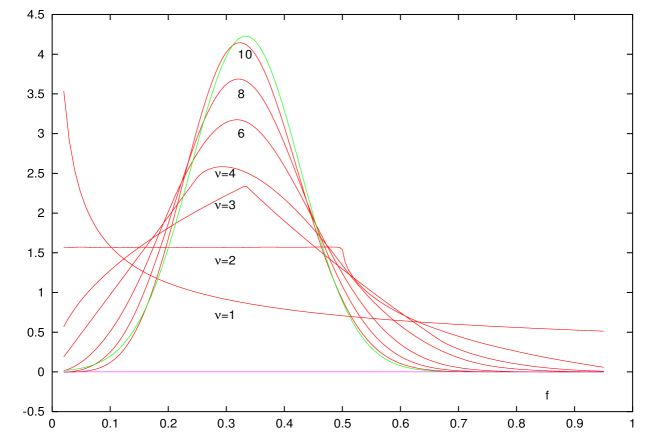
FIG. 1.: Probability distributions $P_{\nu}(f)$ for observing the fraction $f$ of neutral pions in an ensemble of configurations with $\nu$ disoriented domains of size $V/\nu$, according to (16). The dashed line indicates the Gaussian (17) for $\nu=10$.

For $\nu$ such domains of size $V/\nu$ within a source of volume $V$ the probability $P_{\nu}(f)$ to find the fraction $f$ in a given event then is

$$P_{\nu}(f)=\int_{0}^{1}...\int_{0}^{1}\;\delta\left(f-\frac{1}{\nu}(f_{1}+...+f_{\nu})\right)P(f_{1})...P(f_{\nu})\;df_{1}...df_{\nu}$$ (16)

with $P(f)$ given by (15). Some of these functions, for $\nu=1$ to $\nu=10$, are shown in Fig.1. For increasing $\nu$ they approach the Gaussian distribution

$$P_{\nu}(f)=\sqrt{\frac{1}{2\pi\sigma^{2}_{\nu DCC}}}\exp\left(-\frac{(f-\frac{1}{3})^{2}}{2\sigma^{2}_{\nu DCC}}\right)$$ (17)

with width

$$\sigma^{2}_{\nu DCC}=\frac{1}{\nu}\left(\langle f^{2}\rangle-\langle f\rangle^{2}\right)=\frac{1}{\nu}\left(\frac{1}{5}-\frac{1}{9}\right)=\frac{4}{45\nu},$$ (18)

where ”$\langle\rangle$” denotes the expectation value obtained with the single-domain probability (15). Already for $\nu\sim 10$ domains, the distributions (16) are very close to the Gaussian (17), with the maximum shifted only slightly to smaller values of $f$.

For comparison, for uncorrelated sources, the probability to find the fraction $f$ of neutral pions in an ensemble of events each of which emits (the same) total number $n$ of pions, with equal probability $p=1/3$ for each isospin component, is given by the binomial distribution. Its large-$n$ limit is a Gaussian

$$P_{n}(f)=\sqrt{\frac{1}{2\pi\sigma^{2}_{n}}}\exp\left(-\frac{(f-\frac{1}{3})^{2}}{2\sigma^{2}_{n}}\right)$$ (19)

with width

$$\sigma^{2}_{n}=\frac{p(1-p)}{n}=\frac{2}{9n}.$$ (20)

(The multiplicity distributions for neutral or charged pions commonly presented in experimental analyses contain also the event-by-event fluctuations in the total number $n$ of pions. For the discussion of DCC effects it is crucial to look at the event-by-event distribution of ratios, like $f$). The width (20) of the non-DCC distribution decreases with $1/\sqrt{n}$, while the width (18) for $\nu$DCC events seems to be independent of the total number $n$ of pions emitted per event. However, both, the number $\nu=V/v_{D}$ of DCC domains (with fixed average domain volume $v_{D}$) present within the volume $V$, and the total number $n$ of pions emitted from a random source (with fixed emission density $\Gamma=n/V$), are proportional to the total volume $V$ of the fireball. So, in the Gaussian limit, $\nu$ will be proportional to $n$ and we cannot distinguish between (17) and (19). By comparison we find $n=(5/2)\nu$, or $v_{D}=5/(2\Gamma)$. This means that a large fireball consisting of many DCC domains with radii $R_{D}\sim\frac{1}{2}(5/(2\Gamma))^{1/3}$ is equivalent to a random source with emission density $\Gamma$. For a typical value $\Gamma=1$ fm^-3 this radius is about $R_{D}\sim 0.7$ fm. Domains growing beyond that value (for fixed $V$) lead to a broadening of $P(f)$ according to (18). This broadening may occur in the Gaussian limit (especially for large fireballs), where the number $\nu$ of DCC domains present is too large to observe the strong anomalies in the shape of $P_{\nu}(f)$ for very small numbers of $\nu$.

III The model

The 3+1 dimensional $O(4)$ model is defined in terms of the $4$-component field $\mbox{\boldmath$\Phi$}=\Phi\mbox{\boldmath$\hat{\Phi}$}$ with $\mbox{\boldmath$\hat{\Phi}$}\cdot\mbox{\boldmath$\hat{\Phi}$}=1$, and the modulus field $\Phi$ of mass dimension 1, with the following lagrangian density in $3+1$ dimensions

$${\cal{L}}={\cal{L}}_{(2)}+{\cal{L}}_{(4)}+{\cal{L}}_{(0)}$$ (21)

which comprises the kinetic term of the linear $\sigma$ model

$${\cal{L}}_{(2)}=\frac{1}{2}\partial_{\mu}\mbox{\boldmath$\Phi$}\partial^{\mu}\mbox{\boldmath$\Phi$},$$ (22)

the four-derivative Skyrme term

$${\cal{L}}_{(4)}=-\frac{1}{4e^{2}}\left[(\partial_{\mu}\mbox{\boldmath$\hat{\Phi}$}\partial^{\mu}\mbox{\boldmath$\hat{\Phi}$})^{2}-(\partial_{\mu}\mbox{\boldmath$\hat{\Phi}$}\partial_{\nu}\mbox{\boldmath$\hat{\Phi}$})(\partial^{\mu}\mbox{\boldmath$\hat{\Phi}$}\partial^{\nu}\mbox{\boldmath$\hat{\Phi}$})\right],$$ (23)

and the potential

$${\cal{L}}_{(0)}=-\frac{\kappa^{2}}{4}\left(\mbox{\boldmath$\Phi$}^{2}-f^{2}(T)\right)^{2}+H\Phi_{4}.$$ (24)

The transition from a chiral-symmetric ”hot” phase to the ”cold” phase with spontaneously broken chiral symmetry is driven by the coefficient $f^{2}$ which multiplies the quadratic term in the potential (24). Generally speaking, $f^{2}$ is just some input function of time (and space), which is negative in hot and positive in cold areas. If the transition proceeds through at least locally equilibrated states, then $f^{2}$ is a function of the time-dependent (local or global) temperature $T(t)$. We shall formally write $T$ for the argument of $f^{2}$ and call $T$ the ”temperature”, although we should keep in mind that this may be just some parametrization of the input function $f^{2}$ and does not really imply that thermal equilibration is being achieved at every point in time.

We include in the potential an explicitly symmetry-breaking term acting in the intrinsic 4-direction with constant (temperature-independent) strength $H$. The minimum of the potential is located at $\mbox{\boldmath$\Phi$}_{min}=(0,0,0,f_{0}(T))$, related to the coefficient $f^{2}(T)$ of the quadratic term through

$$f^{2}(T)=f_{0}^{2}(T)-\frac{H}{\kappa^{2}f_{0}(T)}.$$ (25)

Small fluctuations around this minimum orthogonal to the 4-direction carry the ”$\pi$-mass” $m_{\pi}$,

$$m_{\pi}^{2}(T)=\frac{H}{f_{0}(T)}$$ (26)

while the fluctuations in 4-direction are characterized by the ”$\sigma$-mass” $m_{\sigma}$

$$m_{\sigma}^{2}(T)=2\kappa^{2}f_{0}^{2}(T)+m_{\pi}^{2}(T).$$ (27)

Conventionally, we define the ”bag field” $\varphi$ by normalizing the modulus of $\Phi$ to its ($T$=0) vacuum value $f_{\pi}=f_{0}(T\to 0)$

$$\mbox{\boldmath$\Phi$}=f_{\pi}\varphi\mbox{\boldmath$\hat{\Phi}$}$$ (28)

such that the bagfield $\varphi$ equals unity in the physical vacuum.

With the physical ($T$=0) values of $f_{\pi}$=93 MeV, $m_{\pi}$=138 MeV, with the standard Skyrme parameter $e$=4.25, the only remaining free parameter in ${\cal{L}}$ is the dimensionless coupling constant $\kappa^{2}$. Through (27) it is related to the ($T$=0) $\sigma$-mass. For the range 6 $<m_{\sigma}/f_{\pi}<$ 10 we find a typical range of 18 $<$$\kappa^{2}$$<$ 50. The spatial extension of a B=1 skyrmion is $(ef_{\pi})^{-1}$, so we will be dealing with baryons of typical (baryonic) size of about 0.5 fm. (Not to be confused with their electromagnetic radii which receive sizable contributions from vector meson clouds.)

IV Roll-down and Domain growth after sudden quench

A Sudden quench

As an input for the classical evolutions the detailed form of the function $f^{2}(T)$ in (24) is needed. If slow cooling proceeds through a sequence of thermally equilibrated states the temperature dependence of the condensate $f_{0}^{2}(T)$ may be obtained from thermal field theory, from loops at the bosonic or the underlying quark level. Typically, for temperatures above a critical temperature $T_{c}$, the condensate $f_{0}(T)$ slowly approaches zero $f_{0}(T/T_{c}>1)\to 0$. According to (25-27), the $\pi$- and $\sigma$-masses then increase and come close to each other, $m_{\pi}/m_{\sigma}\to 1$ for $T/T_{c}>1$, while the second-order coefficient $f^{2}(T/T_{c}>1)$ turns negative with increasing absolute value (cf. Fig.2). Although all of this looks very much like the standard picture of a second-order phase transition, it probably should not be trusted too much near and above $T_{c}$, because the chiral phase transition may be closely related to the color-deconfining transition, so number and nature of the relevant degrees of freedom may change drastically near $T_{c}$, and our basic concept to describe the dynamics in terms of a hadronic order-parameter field may break down.

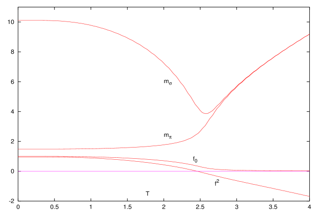
FIG. 2.: Typical features [9] of the condensate $f_{0}(T)$, the coefficient of the quadratic term $f^{2}(T)$ in the $\Phi^{4}$-potential, the pion mass $m_{\pi}$, and the $\sigma$-mass $m_{\sigma}$, as functions of the temperature $T$ for the chiral phase transition. (Energies and temperature in units of $f_{\pi}$.)

However, if the cooling proceeds sufficiently fast as compared to the typical relaxation time $\tau$ of the system we can impose a ”sudden quench” where at time $t$=0 the system is prepared in some hot $T>T_{c}$ initial configuration, and then the ”temperature” is quenched instantly down to $T=0$. Then, for times $t>0$ the system evolves from its high-$T$ initial configuration, subject to the $T$=0 form of the potential (24). Clearly, in this case no assumption about thermal equilibration, even more, no further information on the specific form of $f_{0}(T)$ is needed.

B Initial and boundary conditions

Evolution of $\mbox{\boldmath$\Phi$}_{cl}$ proceeds through the TDGL equations of motion as they result from the potential part of (21), (i.e. also from the Skyrme term only the spatial-derivative terms are kept). As far as the dissipative term originates from elimination of fluctuational modes which simulate a heat bath for the evolving field configuration, addition of fluctuational noise $\xi$ may be required.

With the equations of motion (6) being purely first order in time derivatives it is sufficient to specify for initial conditions at $t=0$ only the field configurations themselves. As time-dependent dynamic fluctuations are not part of $\mbox{\boldmath$\Phi$}_{cl}$ the high-temperature initial configuration is $\mbox{\boldmath$\Phi$}_{cl}\equiv 0$ in the interior of the spatial region in which the hot chiral field is located (apart from a small optional bias in 4-direction due to explicit symmetry breaking), and it takes on the true vacuum values on its boundary. The first step in the time evolution is therefore governed by the stochastic force $\xi$ alone. But this first step will immediately create a configuration $\mbox{\boldmath$\Phi$}_{cl}$ which is of stochastic nature itself. Therefore, choosing each of the four cartesian field components at each interior point of the lattice from a random Gaussian deviate, and fixing $\mbox{\boldmath$\Phi$}=(0,0,0,f_{\pi})$ on the boundary of the lattice, provides convenient initial configurations with spatial correlation length less than one lattice unit. The width $\Delta$ of the Gaussian deviate reflects the initial temperature $T>T_{c}$. It is not really necessary to specify a definite value for this temperature because after about one relaxation-time unit (after the sudden quench) the details of the initial configuration are lost anyway and evolutions proceed quite similarly, for widths chosen in the range $0.1<\Delta/f_{\pi}<0.5$. Numerically, very small values of $\Phi$ (i.e. small values of the width $\Delta$) require very small timesteps at the beginning, therefore for convenience we generally choose $\Delta/f_{\pi}=0.3$. The $(T=0)$ vacuum boundary conditions

$$\mbox{\boldmath$\Phi$}(t)=(0,0,0,f_{\pi})$$ (29)

are kept fixed for all times at the lattice surface. This allows compactification of 3-space to a 3-sphere $S^{3}$, and guarantees integer winding numbers.

Starting from these initial conditions events are generated by evolving the configurations according to the TDGL eq.(6). Because the time scale enters only through the $\dot{\mbox{\boldmath$\Phi$}}$ term, it is convenient to measure the time in relaxation-time units $\tau$. A large number of events generated in this way constitute the statistical ensemble from which ensemble averages then can be obtained at some point in time during the evolution.

C Conservation of baryon number

The topological current is

$$j_{\mu}=\frac{1}{12\pi^{2}}\epsilon_{\mu\nu\rho\sigma}\epsilon_{abcd}\hat{\Phi}_{a}\partial^{\nu}\hat{\Phi}_{b}\partial^{\rho}\hat{\Phi}_{c}\partial^{\sigma}\hat{\Phi}_{d}$$ (30)

which satisfies $\partial^{\mu}j_{\mu}=0$. It allows to assign a value $\rho(i,j,k)$ of the winding density $\rho\equiv j_{0}$ to each point $(i,j,k)$ of the cubic lattice (or, more precisely, to each elementary lattice cube with lowerleft corner $(i,j,k)$) such that the total winding number

$$B=\sum_{i,j,k=0}^{L-1}\rho(i,j,k)$$ (31)

summed over the whole lattice is integer and configurations can be selected with some desired integer value of $B$. We also define

$$N=\sum_{i,j,k=0}^{L-1}|\rho(i,j,k)|$$ (32)

by summing up the absolute values of the local winding densities. Of course, $N$ generally is not an integer. However, if a configuration describes a distribution of localized textures (and antitextures) which are sufficiently well separated from each other, then $N$ is close to an integer and counts the number of these textures (plus antitextures). In that case we can define the numbers $N_{+},N_{-}$ of ”baryons” and ”antibaryons” through

$$B=N_{+}-N_{-}~{}~{}~{}~{}~{}~{}~{}~{}~{}~{}~{}N=N_{+}+N_{-}~{}~{}.$$ (33)

Even if it is not integer we will in the following sometimes briefly call $N$ the ”number of baryons plus antibaryons”.

In a lattice implementation the local update of $\mbox{\boldmath$\Phi$}(i,j,k)$ at some timestep at some lattice point $(i,j,k)$ will occasionally lead to a discrete jump in the total winding number $B$. For well-developed localized structures this corresponds to unwinding textures or antitextures independently, such that $B$ decreases or increases by one or more units. This will eventually happen even for implementations of the nonlinear $O(4)$-model where the length $\Phi$ is constrained to $f_{\pi}$ and $B$ is topologically conserved, because the topological arguments based on continuity do not apply to the discrete lattice configurations. It can be prevented by an (optional) $B$ filter which rejects such a $B$-violating local field update at that lattice point and timestep. This eliminates all independent unwinding processes. Only simultaneous annihilation of texture and antitexture in the same time step remains possible, and, as the update proceeds locally at each lattice vertex it can happen only if texture and antitexture overlap. This $B$-conserving evolution is characteristic for the nontrivial topology of the nonlinear $O(4)$-model and in this way can be implemented as an optional constraint also into the linear $O(4)$-model. In the continuum limit it implies that a vanishing modulus $\Phi=0$ of the field vector is excluded.

Practically, during the very early stages of an evolution, where the local gradients of the angular fields still are of the order of $\pi/a$, (where $a$ denotes the lattice constant), annihilation processes by far exceed local unwinding, and cause a very rapid decrease of the initially large number $N$. During that stage the definition of the global baryon number $B$ requires a prescription of how to define the baryon number located on one elementary lattice cube (which necessarily involves some arbitrariness like mapping on geodesics). If the lattice constant $a$ is chosen sufficiently small (as compared to the typical spatial size $R=(ef_{\pi})^{-1}=0.5$ fm of stable $B=1$ baryons) such that the emerging localized extended structures are described with reasonable accuracy on the lattice, the small global baryon number $B$ stabilizes very quickly and local unwinding no longer occurs. It turns out that $R/a=3$ is sufficient to avoid the need for imposing an explicit constraint on $B$. This implies a lattice constant of $a=1/6$ fm, which appears as a reasonable value for the lattice implementation of an effective low-energy model.

As there is no universal simple scaling law (due to the ocurrence of different powers of gradients in ${\cal{L}}$, or in other words, due to explicit scales introduced through soliton size and symmetry breaking) changes of the lattice constant can only partly be absorbed into corresponding changes in the time scale, and we have to check to which extent physical statements, like the physical size of oriented domains at the time when the roll-down is completed, are independent of the choice of the lattice constant $a$ (for a fixed physical size $(aL)^{3}$ of the finite total volume).

D Angular correlations

A convenient measure for the average size $R_{D}$ of (dis)oriented domains is the half-maximum distance $R_{1/2}$ of the equal-time lattice averaged angular correlation function

$$C(R)=\left[\underbrace{\sum_{i,j,k=0}^{L}\ \sum_{l,m,n=0}^{L}}_{\delta\leq R<\delta+1}\mbox{\boldmath$\hat{\Phi}$}(i,j,k)\cdot\mbox{\boldmath$\hat{\Phi}$}(l,m,n)\;/\underbrace{\sum_{i,j,k=0}^{L}\ \sum_{l,m,n=0}^{L}}_{\delta\leq R<\delta+1}\ 1\right]-\langle\mbox{\boldmath$\hat{\Phi}$}\rangle^{2}$$ (34)

$${\rm with}\qquad\delta=\sqrt{(i-l)^{2}+(j-m)^{2}+(k-n)^{2}}$$

Note that the definition (34) contains only the unit vectors $\hat{\Phi}$, and not the full field vectors $\Phi$, i.e. $C(R)$ measures only the angular correlations in a given configuration. The half-maximum distance $R_{1/2}$ is conveniently obtained by interpolating between the two neighbouring integer values of $R$ where $C(R)$ passes through $C(0)/2$. This lattice averaged correlation length can be obtained as function of time for any individual configuration (in a statistical ensemble of many events) and compared to the domain pattern of that same individual configuration. Analysing the domain sizes shows that $R_{D}\approx R_{1/2}$ provides a reasonable measure for the average size $R_{D}$ of (dis)oriented domains. To extract an accurate growth law for $R_{D}$, of course, would require to perform an additional ensemble average at each point in time, but for a sufficiently large lattice the spread in $R_{1/2}(t)$ for different events is small (as long as $R_{1/2}<L/2$), and it is sufficient to study $C(R)$ on an event-by-event basis.

Explicit symmetry breaking (through nonvanishing $H$ in (24), and through the vacuum boundary conditions (29) imposed on $\Phi$) causes a nonzero average $\langle\mbox{\boldmath$\hat{\Phi}$}\rangle$ growing (in 4-direction) with time, so on a finite lattice at late times it becomes numerically inconvenient to extract $R_{1/2}$ from $C(R)$. Therefore, in analogy to (34), we define a correlation function $C_{\pi}(R)$

$$C_{\pi}(R)=\underbrace{\sum_{i,j,k=0}^{L}\ \sum_{l,m,n=0}^{L}}_{\delta\leq R<\delta+1}\mbox{\boldmath$\hat{\Phi}$}_{\pi}(i,j,k)\cdot\mbox{\boldmath$\hat{\Phi}$}_{\pi}(l,m,n)/\underbrace{\sum_{i,j,k=0}^{L}\ \sum_{l,m,n=0}^{L}}_{\delta\leq R<\delta+1}\ 1$$ (35)

where $\mbox{\boldmath$\hat{\Phi}$}_{\pi}$ is the ”pionic” (orthogonal to the 4-direction) part of $\hat{\Phi}$, renormalized to form a 3-dimensional unit vector $\mbox{\boldmath$\hat{\Phi}$}_{\pi}\cdot\mbox{\boldmath$\hat{\Phi}$}_{\pi}=1$. The function $C_{\pi}(R)$ measures the angular correlations in the pionic 3-space orthogonal to the 4-direction, unaffected by explicit symmetry breaking. It satisfies $C_{\pi}(0)=1$, and the corresponding half-maximum radius will be denoted as $R_{\pi}$.

The angular ordering is driven by the terms ${\cal{L}}_{(2)}$ and ${\cal{L}}_{(4)}$, which contain two, respectively four, angular gradients. From simple scaling arguments we expect each of these terms, separately, to lead to $t^{1/2}$, respectively $t^{1/4}$, power-laws for the growth of the spatial scale of disoriented domains. However, their relative strength introduces a definite scale into the system (the size $(ef_{\pi})^{-1}$ of the baryons), and the presence of extended textures will cause deviations from the scaling growth laws.

V Results

A Roll-down times

As a global measure for the restoration of the chiral condensate we consider the lattice average of the modulus of the order parameter field $\langle\varphi\rangle$. In the interior of stable baryons the $\varphi(\mbox{\boldmath$x$},t)$-field will stay small (constituting the bags), while in the exterior region it will evolve towards the vacuum value $\varphi$=1. Depending on the size $R^{3}$ and number $N$ of baryons (+ antibaryons) which finally stabilize inside the total volume $(aL)^{3}$, the average $\langle\varphi\rangle$ will approach a value near $1-N(R/aL)^{3}$. We define the typical roll-down time $t_{RD}$ as that point in time after the sudden quench when $\langle\varphi\rangle$ has reached 80% of its final value. Locally, the roll-down towards the vacuum value $\varphi$=1 in the exterior regions is driven by the potential part ${\cal{L}}_{(0)}$ (24) of ${\cal{L}}$. Therefore, for a large lattice, as long as the baryon(+antibaryon) density is small, we expect $t_{RD}$ to scale with $\kappa^{-2}$, i.e. with the inverse strength of the $\Phi^{4}$-potential. The typical range for the ($T$=0) $\sigma$-mass ( $6<m_{\sigma}/f_{\pi}<10$ ) provides limits for $\kappa^{2}$ ($18<\kappa^{2}<50$). This constitutes a relatively weak potential to compete with the gradient terms in ${\cal{L}}$, so we expect deviations from a pure $\kappa^{-2}$-power law. Similarly, the actual roll-down times are significantly reduced through the symmetry-breaking imposed by the finite pion mass and the vacuum boundary conditions which become increasingly important for smaller lattices. We find typical roll-down times of the order of $t_{RD}/\tau\approx$ 2-3 (for $\kappa^{2}=50$ and lattice sizes $L=30-60$) and $t_{RD}/\tau\approx$ 5-8 for ($\kappa^{2}=20$). This shows that the potential part indeed has a dominating influence for the evolution of the chiral condensate. The slight prolongation of $t_{RD}$ with increasing lattice size $L$ reflects the influence of the vacuum boundary condition on the growth of $\Phi$ in the interior of the volume.

B Features of the evolutions

Evolutions after a sudden quench show three typical distinguishable phases:

I.) During the first phase, which extends to about $t/\tau\sim 0.1-0.2$ after the quench, the initially random configuration quickly aligns locally, such that the angular correlation lengths $R_{D}\approx R_{\pi}$ grow to about 3-4 lattice units (corresponding to about 0.5-0.7 fm).

FIG. 3.: Typical field configurations during the early phase (I), at times $t/\tau$=0.02 and $t/\tau$=0.1 after the sudden quench. The arrows show the isospin (unit-)vectors at the lattice points of a 2-dimensional cut through a 60³ cubic lattice, projected on a plane in isospace.

Fig.(3) shows a 2-dimensional cut through a 60³ cubic lattice with the isospin (unit)-field vectors projected into a plane in isospace, at times $t/\tau=$ 0.02 (where local aligning is already clearly visible), and at $t/\tau=$ 0.1, which approximately marks the end of this first phase. The condensate $\langle\varphi\rangle$ does not grow during this period, in fact, the lattice average decreases to a minimum slightly below its small initial value. The total baryon-plus-antibaryon number $N$ (which is becoming really well-defined only towards the end of these very early stages) drops to values of about 100-200 on a $L$=60 lattice, corresponding to a (baryon+antibaryon) density of 0.1-0.2 fm^-3, while the integer baryon number $B$ is close to or equal to zero. Already by the end of this short first phase the winding density has developed pronounced maxima and minima at the locations of the emerging (anti-)baryons, while the bag field $\varphi$ drops smoothly from its vacuum boundary condition to its small value throughout the interior volume, and develops dips near the extrema of the winding density. All of these features are basically independent of the $\Phi^{4}$-potential strength $\kappa^{2}$, the total volume $L^{3}$, and the symmetry breaking. The latter, however, causes a steady increase in the lattice average $\langle\Phi_{4}\rangle$ of the 4-component of the vector field $\Phi$, which initially is very close to zero. The energy density $e=U/(aL)^{3}$ in the random configuration at time $t$=0 is extremely high (of the order of 10-50 GeV/fm³), and located almost completely in the angular gradients of the Skyrme term ${\cal L}^{(4)}$. (Note that the energy density $e_{V}=(\kappa^{2}/4)f_{\pi}^{4}$ located in the $\Phi^{4}$-potential for $\Phi\equiv 0$ is only about $e_{V}$=0.05 GeV/fm³ for $\kappa^{2}=20$.) By the end of this first phase the energy density has dropped to values of about 0.3-0.5 GeV/fm³, i.e. to values where we might hope that this effective hadronic model may become reasonable to apply. So we may conclude that this first phase of the evolutions rather serves to create an ensemble of initial conditions for the onset of the physically reasonable time-development of the model which begins near $t/\tau\approx 0.1$ after the sudden quench with correlation lengths of the order of 0.5 fm.

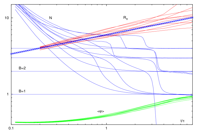
FIG. 4.: Particle numbers $N$, winding numbers $B$, correlation lengths $R_{\pi}$ (in lattice units), and average condensates $\langle\varphi\rangle$, for a sample of ten events during the roll-down phase (II) after a sudden quench. For comparison, the straight line (with crosses) indicates the power law $6t^{0.25}$). The evolutions proceed on a $L=30$ cubic lattice, with potential strength $\kappa^{2}=20$.

II.) The second (’roll-down’) phase is characterized by the growth of the local $\varphi$-field towards unity in the spatial regions between the emerging baryons, so the lattice averaged condensate $\langle\varphi\rangle$ increases towards its final value. As discussed above, the duration of this roll-down phase is dominated by the strength of the $\Phi^{4}$ potential and by symmetry breaking. Fig.(4) shows a sample of ten events evolving on an $L=30$ lattice with lattice constant $a=(1/3)(ef_{\pi})^{-1}=0.167$ fm, $\kappa^{2}=20$, and $m_{\pi}=138$ MeV, with vacuum boundary conditions after a sudden quench. By the time of $t/\tau=0.1$ the total ’particle’ numbers have dropped to $N\sim$ 15-20 and keep falling rapidly until after some final annihilations they approach the fixed (net baryon) winding numbers $B$, which scatter between 0 and 4 in this sample. The growth of the average condensate $\langle\varphi\rangle$ is very similar for all events and differs only through slightly varying final values due to the different baryon numbers.

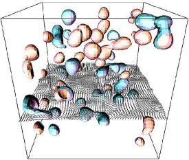
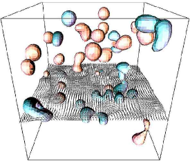
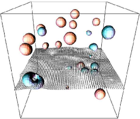
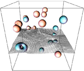
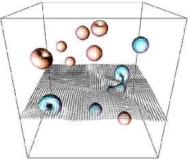
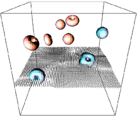
FIG. 5.: Snapshots of surfaces of equal (absolute) values of winding densities during and beyond the roll-down phase ($t/\tau$=0.4, 0.8, 4.0, 8.0, 20, 40 from upper left to lower right) for a single event evolving after a sudden quench on a $L$=60 cubic lattice with $\kappa^{2}$=20. In an arbitrarily selected 2-dimensional cut through the lattice the isospin (unit-)vectors are also plotted to show the growth of aligned domains.

The angular ordering increases by moving the boundaries of oriented domains, by further annihilations, or fusion of individual baryons into more complex multi-$B$ configurations. As long as such extended localized textures are present, they prevent straight alignment of the isovector part of the field in the spatial domains which surround and separate them, while the 4-components follow the driving symmetry breaker towards the aligned vacuum. Therefore, the growth of the angular correlation length $R_{\pi}$ is quite slow. During the roll-down phase it follows approximately a power growth law $t^{\alpha}$ with $\alpha$ varying between 0.25 and 0.3, as we might expect from the separate or at least dominant acting of the Skyrme term. Due to this slow growth, the average radius $R_{\pi}$ of aligned disoriented domains in isospace reaches only about 7 to 10 lattice units at roll-down time $t_{RD}$, and differences in $t_{RD}$ due to different choices of $\kappa^{2}$ do not lead to sizeable differences in $R_{\pi}$ by the end of this roll-down period. Depending on the baryon number remaining in the configurations after roll-down, the angular pionic correlation lengths $R_{\pi}$ either saturate near 10 lattice units, or (for $B=0$) keep rising towards lattice size. However, by that time, the topologically trivial domains of the whole field are already oriented in 4-direction, the condensate $\langle\Phi\rangle$ is saturated by $\langle\Phi_{4}\rangle$, i.e., the pionic components $\Phi_{i}$ for $i$=1,2,3 in the aligned domains practically vanish. In other words, outside of stable textures the field is aligned in vacuum direction before the (T=0) condensate is fully restored. The same holds also for the stronger potential $\kappa^{2}=50$ (i.e. $m_{\sigma}/f_{\pi}\sim 10$).

III.) The final part of the evolution after completion of the roll-down is characterized by the stable textures approaching their minimal-energy configurations. Occasionally, some final annihilations may occur, and due to mutual attraction the locally separated baryons drift towards each other and finally combine into the multi-$B$ ’nuclei’ which constitute the classical minimal-energy configurations of the model lagrangian (21). On the relaxation-time scale this is an extremely slow process which extends over $\sim 10^{3}$ relaxation time units, with correspondingly small field velocities. So, from the point of pion emission abundances, it is uninteresting. Furthermore, with propagating terms included in the classical equations of motion, the individual baryons or antibaryons would be able to leave the volume before fusing into multi-$B$ configurations.

In order to convey a more pictorial view of the field evolutions we plot in figs.(5) 3-d views of the winding densities $\rho_{0}$ from eq.(30) at six different times $t/\tau$=0.4, 0.8, 4, 8, 20, 40, which cover the roll-down period for an individual evolution on a 60³ lattice. The surfaces plotted show the equal-(positive or negative)-density surfaces, so baryons and antibaryons can be distinguished. Each snapshot contains also an arbitrarily selected plane in which the isospin field (unit-)vectors are plotted as short lines, so the growth of aligned domains is clearly visible. Evidently, already at the beginning of the roll-down, the individual (anti-)baryons are separately developed, and while the average condensate is growing towards its vacuum value, the angular ordering proceeds mainly through annihilation and fusion, where in this specific example several $B=2$ torus configurations and one $B=4$ cluster are created.

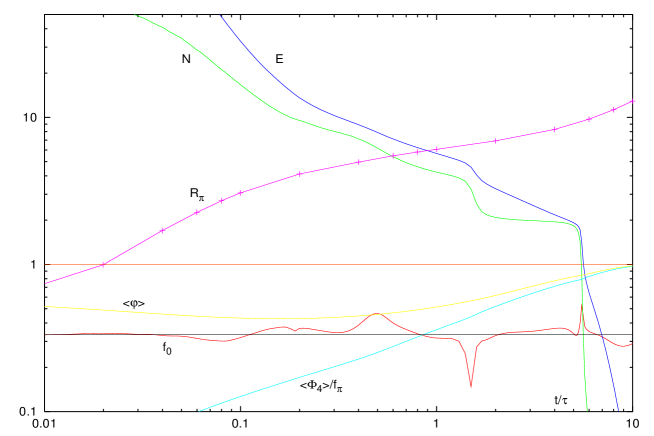
FIG. 6.: Particle number $N$, total energy $E$ (in units of $6\pi^{2}f_{\pi}/e$), correlation length $R_{\pi}$ (in lattice units), average condensate $\langle\varphi\rangle$, average 4-component $\langle\Phi_{4}/f_{\pi}\rangle$, and the abundance ratio $f_{0}$ for neutral pion emission, obtained from the field velocities according to eq.(8-10), for one single event during the roll-down phase (II). The evolution proceeds on an $L=30$ cubic lattice after a sudden quench, with potential strength $\kappa^{2}=20$.

C Pion abundance ratios

Within our approximation scheme, the abundance of neutral pions emitted relative to all pions is given by the ratio of the averaged square of the field velocities (8-10). In Fig.(6) we look at one typical single event evolving on a $L=30$ lattice like the sample shown in Fig.(4). It is characterized by baryon number $B=0$. The baryon-plus-antibaryon number approaches the integer value $N$=2 near $t/\tau\sim 1$, the final annihilation process takes place between $t/\tau$=5 and $t/\tau$=6. By that time the average condensate $\langle\varphi\rangle$ has reached 80% of its final value, while the average $\langle\Phi_{4}/f_{\pi}\rangle$ has almost caught up with $\langle\varphi\rangle$, i.e. even before the roll-down is finished, the field surrounding the last two remaining baryons is essentially oriented in 4-direction. During the roll-down phase from $t/\tau\approx 0.2$ until $t/\tau\approx 6$ the correlation length $R_{\pi}$ grows according to 6$t^{0.25}$ and reaches about 10 lattice units at roll-down time. Only after the final annihilation the growth rate accelerates.

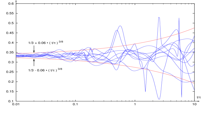
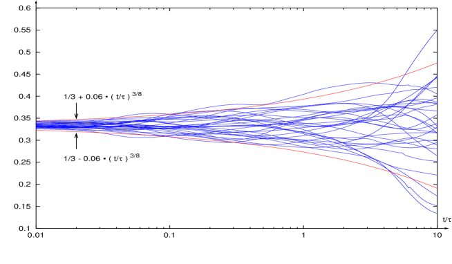
FIG. 7.: a) The abundance ratios $f_{0}[\dot{\Phi]}$ for neutral pion emission, obtained from the field velocities according to eqs.(8-10) for a sample of 10 events evolving on an $L=30$ lattice with $\kappa^{2}=20$. The lower part b) shows for the same sample the ratios $f_{i}[\Phi]$ for all three isovector components $i=1,2,3$, obtained from the field configurations according to eq.(36). For comparison the growth law $1/3\pm 0.06(t/\tau)^{3\alpha/2}$ for $\alpha=0.25$ is included.

Figure (6) includes the abundance ratio $f_{0}[\dot{\Phi}]$ for neutral pion emission, obtained from the field velocities as given in eqs.(8) and (10). The velocity-dependent $f_{0}[\dot{\Phi}]$ shows a few pronounced extrema, which are clearly correlated with major reordering in the topological structures, i.e. in this case $B-\bar{B}$ annihilations. Otherwise $f_{0}$ shows small fluctuations around the average value of 1/3. We expect that for anomalies in pionic abundance ratios the sizes of aligned domains with different orientations of their isospin (1,2,3)-field components are important. Apart from the specific fluctuations in the velocities which occur in connection with annihilation or fusion processes of the emerging baryons, the pionic abundance ratios calculated from averaging the square of the field velocity components (10), or by averaging the square of the field components

$$f_{i}[\Phi]=\frac{\langle\Phi^{2}_{i}\rangle}{\sum\limits_{j=1,2,3}\langle\Phi^{2}_{j}\rangle}.$$ (36)

show comparable deviations from the average value of 1/3. According to (18) the widths $\sigma_{\nu DCC}$ of these latter deviations (36) grow with $1/\sqrt{\nu}$. The number $\nu$ of aligned disoriented domains decreases as $R_{\pi}^{-3}\propto(t^{\alpha})^{-3}$, i.e. $\sigma_{\nu DCC}$ grows like $\sim t^{3\alpha/2}$. (In this consideration we neglect that the effective volume available for disoriented domains is only the difference between the total volume and that part which is already fully aligned in 4-direction). In Figs.(7a,b) we compare the ratios $f_{0}[\dot{\Phi}]$ and $f_{i}[\Phi]$ for a sample of events. Evidently, apart from the sporadic peaks in $f_{0}[\dot{\Phi}]$ due to $B-{\bar{B}}$ annihilations both distributions are reasonably well bound by the $t^{3\alpha/2}$ law which links them to the growing size of disoriented domains.

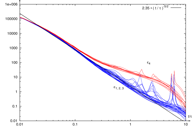
FIG. 8.: The rates of energy loss $\epsilon_{a}$ (8) (for $a$=1,2,3 and $a=4$) through emission of pions and $\sigma$-mesons for a sample of 10 events evolving on an $L=30$ cubic lattice after a sudden quench, with potential strength $\kappa^{2}$=20. For comparison the power-law 2.35 $(t/\tau)^{-2.5}$ is indicated by the straight line.

Despite this significant growth of the width of abundance ratio distributions for neutral pions, observable consequences are strongly suppressed by a rapid decrease of the absolute pion yield rates during the roll-down phase. As obtained according to eq.(8) from the square of the instantaneous field velocities the emission rates $\epsilon_{a}$ for $a$=1,2,3,4 are shown in Fig.(8) for the same sample as in Fig.(7). These rates decrease by three to four orders of magnitude during the roll-down phase, whereby the explicit symmetry breaking enhances the time-derivatives of the 4-component in such a way that the time-integrated rates $\int\epsilon_{4}dt$ are comparable to the sum of the three pionic components $\sum_{i=1,2,3}\int\epsilon_{i}dt$ (integrated over the roll-down phase). During this time interval the pionic emission rates (unaffected by explicit symmetry breaking) decrease approximately like $\sim t^{-\beta}$ with $\beta\approx 2.3-2.5$.

The observed total number $n$ of all pions emitted in a single event is given by the time integral

$$n=\int_{t_{0}}^{\infty}{\dot{n}}(t)dt=\int_{t_{0}}^{\infty}\sum_{i=1,2,3}\epsilon_{i}(t)/m_{\pi}dt.$$ (37)

where the initial time $t_{0}$ marks the onset of the emission. If we approximate the instantaneous emission rate ${\dot{n}}(t)$ for pions emitted from a source of volume $V$ by a power law ${\dot{n}}(t)=\gamma V\>(t/t_{0})^{-\beta}$, with constant emission rate density $\gamma$, we have

$$n=\frac{\gamma V}{(\beta-1)}t_{0}.$$ (38)

If we choose for $t_{0}$ the onset of the roll-down phase, we find for the total energy $E$ at that time typically $E(t_{0}/\tau\sim 0.1)\approx 0.3{\mbox{ GeV/fm}}^{3}~{}(La)^{3}$. With lattice constant $a=1/6$ fm and lattice size $L=60$ the total energy of about 300 GeV residing at time $t_{0}$ in this (10 fm)³ fireball would be dissipated through emission of about 150 GeV/$m_{\pi}\approx 1100$ low-energy pions and 150 GeV/$m_{\sigma}$ $\sigma$-mesons. With $\beta=5/2$, we obtain for the initial pion emission density at time $t_{0}/\tau=0.1$, $\gamma\tau\approx 16$ fm^-3. Evidently, most of the observed pions are emitted at the very beginning of the roll-down phase.

For a random (non-DCC) source the width of the probability distribution for the fraction $f$ of neutral pions is given by the binomial result

$$\sigma_{non-DCC}^{2}=\frac{2}{9n}$$ (39)

where the total number $n$ of pions emitted now is given by (38). For a source with $\nu(t)$ DCC domains present at time $t$ the width of the probability distribution for the observed fraction $f$ of all neutral pions emitted in that event is (with (18))

$$\sigma_{DCC}^{2}=\frac{1}{n}\int_{t_{0}}^{\infty}{\dot{n}}(t)\left(\frac{4}{45\nu(t)}\right)dt.$$ (40)

If the number $\nu(t)$ of DCC-domains present at time $t$ within the volume $V$ is approximated by the power law $\nu(t)=\nu_{0}\>(t/t_{0})^{-3\alpha}$, where $\nu_{0}$ denotes the number of DCC-domains present at time $t_{0}$, we have

$$\sigma_{DCC}^{2}=\frac{4}{45\>\nu_{eff}},~{}~{}~{}~{}~{}{\mbox{ with }}\nu_{eff}=\left(\frac{\beta-3\alpha-1}{\beta-1}\right)\>\nu_{0}.$$ (41)

For positive values of $\alpha$ the effective number of DCC-domains $\nu_{eff}$ is reduced as compared to the number $\nu_{0}$ of domains present at the time $t_{0}$ of the onset of pion emission. (Of course, we have assumed here that the Gaussian approximation remains valid as long as there is noticeable emission strength ${\dot{n}}(t)$. If, however, the growth rate $3\alpha$ of the average volume of one DCC-domain is comparable to ($\beta-1$), the effective number $\nu_{eff}$ becomes very small, the Gauss approximation breaks down, and we may expect the anomalies which characterize $P_{\nu}(f)$ for very small values of $\nu$ as shown in Fig.(1)).

The simulations indicate that $\beta\approx 2.3-2.5$ and $\alpha\approx 0.25-0.3$, so we find

$$\nu_{eff}/\nu_{0}=0.175-0.5$$ (42)

which implies a broadening of the distribution $P(f)$ by a factor of $1.4-2.4$ as compared to the distribution at time $t_{0}$. It may be noted that this result is quite sensitive to the actual values of $\alpha$ and $\beta$: a growth rate of the angular correlation length $R_{\pi}\sim t^{1/3}$ instead of $t^{1/4}$, and the emission rates decreasing like $t^{-2}$ instead of $t^{-2.5}$, would lead to the limiting case $3\alpha=\beta-1$. Unfortunately, the result (41) provides only a relative statement between the observed width $\sigma_{DCC}$ and a hypothetical width at time $t_{0}$, and not a comparison with the width (39) for a binomial distribution. We could enforce such a connection by assuming that for $\alpha=0$ (zero growth rate for DCC domains) the source should be undistinguishable from a randomly emitting source. In that case we would have

$$\sigma_{DCC}=\sigma_{non-DCC}\sqrt{\left(\frac{\beta-1}{\beta-3\alpha-1}\right)}.$$ (43)

So, the growth of the DCC domains, in competition with the decrease of the emission rates, still would lead to a significant broadening in the effective distribution of $\pi_{0}$-abundance ratios, as compared to the corresponding width (39) for a random non-DCC source.

The growth law for the angular correlation length $R_{\pi}$ and the roll-down times $t_{RD}$ are not very sensitive to the (sufficiently large) total lattice size $L$, therefore the width $\sigma_{DCC}$ of the abundance ratio distributions scales with $L^{-3/2}$. (The same holds for the binomial distribution). On the other hand, the amplitudes of pronounced peaks in the abundance ratios $f_{0}[\dot{\Phi}]$ due to restructuring textures, i.e. $B-{\bar{B}}$ annihilation, are independent of $L$, while their number scales with $L^{3}$. So in larger fireballs we would expect additional broadening of the width of fluctuations around the value of 1/3 to be increasingly due to annihilations of nascent baryon-antibaryon structures, without the specific anomalies which characterize pion emission from large disoriented domains.

D Slow cooling

Up to now we have discussed the extreme case of a sudden quench where the potential (24) at time $t=0$ drops instantly to its temperature $T=0$ shape, i.e. $f_{0}^{2}(T)=f_{\pi}^{2}$ for $t>0$. Practically, however, for a smooth quench it may take a typical cooling time $\tau_{c}$ for $f_{0}^{2}(T)$ to approach its $T=0$ value $f_{\pi}^{2}$. As long as $\tau_{c}$ is small as compared to the typical relaxation times $\tau$ of the system, the evolutions proceed much like those for a sudden quench. Noticeable differences appear only if the cooling time $\tau_{c}$ becomes comparable to the typical roll-down time $t_{RD}$ following the sudden quench.

In addition to the smooth time-dependence of $f_{0}(T(t))$, the field configurations may be subjected to a stochastic force which describes the back-reaction of the eliminated fluctuations on the slowly evolving degrees of freedom, acting as a heat bath for the cooling fireball. As we have assumed in eq.(8) that the main source of energy loss is through pion and $\sigma$ emission, with the fireball immersed in the $T=0$ vacuum, the strength of the stochastic force is not strictly tied to the relaxation constant $\tau$, but will be comparatively small. Let us therefore separately discuss the influence of the smoothly time-varying coefficient $f^{2}$ in the $\Phi^{4}$-potential, without any noise term.

The first phase (I) of the ordering evolution proceeds independently from the strength of the $\Phi^{4}$ potential, so it is also insensitive to the actual value of $f^{2}(T)$. The angular correlation lengths and the baryon-plus-antibaryon densities established by the end of this phase are independent of the cooling time $\tau_{c}$.

Subsequently, during the roll-down phase (II) of a slow cooling process with $\tau_{c}\gg t_{RD}$, the configurations which emerge near the end of phase (I) now have sufficient time to relax towards a minimum at the instantaneous temperature. As a result of the baryon radius $R$ scaling as $R\sim(ef_{0}(T))^{-1}$, with $f_{0}(T)/f_{\pi}<1$ throughout most of the interior volume, the nascent textures are slightly larger, overlap and interact more strongly, and therefore annihilate or fuse more easily into multi-$B$ configurations. All these textures are well developed by the end of phase (II) although the actual condensate $\langle\Phi\rangle$ is close to the momentaneous value of $f_{0}(T(t))$, i.e. much smaller than $f_{\pi}$.

During the following increase of $\langle\Phi\rangle$ towards $f_{\pi}$ which proceeds on the time scale $\tau_{c}$, the established configurations simply follow the changing effective potential in a more or less equilibrated manner. The addition of a small temperature-dependent noise term causes only a slight retardation in the ordering evolutions.

Altogether, the angular ordering proceeds on the time scale of the relaxation constant $\tau$, quite independently of the cooling time scale $\tau_{c}$. From the point of DCC effects, the case of the sudden quench shows the essential features. The late-time reshaping of the established textures according to a changing $f_{0}(T(t))$ is not relevant for the observability of DCC pion anomalies.

VI Conclusion

As a dynamical model for the relaxation of a hot chirally symmetric ’fireball’ towards the cold vacuum characterized by spontaneously broken chiral symmetry with nonvanishing chiral condensate, we have investigated the classical time evolution of chiral $O$(4)-field configurations. Starting from stochastic initial conditions, which are chirally symmetric in the interior of a finite spatial volume, the evolutions of the classical fields follow purely dissipative dynamics in their relaxation towards the physical vacuum which surrounds the considered volume as boundary condition.

The model is limited by a severe restriction: The chiral $O$(4)-field comprises all degrees of freedom of the relaxing fireball. This renders it questionable that the model can be applied and trusted at conditions which may prevail at temperatures close to or above the critical $T_{c}$ of the chiral phase transition. Consequently, we do not pay much attention to details of the initial conditions. The dissipative dynamics wipes them out, anyway, after a small fraction of the typical relaxation time unit. But we hope, that once the color degrees of freedom are (re-) confined into the hadronic chiral field, and the energy-density has dropped to less than 1GeV/fm³, then the model may provide a reliable picture for the later stages of the evolution when the actual roll-down of the order parameter takes place.

While the dissipative term during the very early phase of the evolution may originate from the rapid expansion of the hot fireball, we assume that during the subsequent roll-down phase energy is lost and carried away by emission of chiral field quanta (pions and $\sigma$-mesons). Then the square of the instantaneous local field velocities provide a measure for the strength of the emitted radiation. Two features are of specific interest: The growth and typical size of domains with disoriented chiral field, and the possibility to observe anomalies in the abundance ratios of emitted pions caused by the transient formation of such domains.

On the other hand, the model is sufficiently sophisticated to allow for creation, stabilization and mutual interactions of baryons and antibaryons in the hot hadronic gas, and their presence as extended topological textures is of specific importance for the ordering process. We consider it as one of the essentials of the present investigation to use an effective action which incorporates the possibility to create and stabilize these structures, because it is well known that textures are of crucial importance for the phenomenology of phase transitions. Their physical size and properties set the scale for the stabilizing and for the explicitly symmetry-breaking terms in the effective action. Numerical implementation on a 3+1 dimensional lattice then requires a lattice constant $a$ which allows to describe these textures with appropriate accuracy. It turns out that $a$=1/6 fm is sufficient for that purpose. Typical fireball diameters in heavy-ion collisions in the range from 5 to 15 fm then require lattice sizes of about $30<L<90$, which are numerically reasonable to handle.

The essentials of our results are the following:

During the very early stages of the evolutions the angular gradient terms which drive the local aligning of the field vectors dominate over the $\Phi^{4}$ potential such that the actual roll-down of the modulus $\Phi$ towards its vacuum value sets in only after angular correlation lengths of about 0.5-0.7 fm have been established (see Fig.(3c), and see the angular correlation radii $R_{\pi}$ in Fig.(4) near $t/\tau$=0.1-0.2). These configurations set the stage for the subsequent roll-down.

During the roll-down phase the angular ordering is dominated by the higher-order gradient terms in the effective action which try to establish low-energy configurations for the emerging extended textures. This leads to an appreciable reduction in the growth exponent $\alpha$ of the angular correlation length $R_{\pi}$, which measures the size of aligned disoriented domains in the isospin subspace, i.e. orthogonal to the 4-direction. Due to this slow growth, the correlation lengths $R_{\pi}$ reach values of only up to about 10 lattice units by the end of the roll-down phase (depending on the number of remaining baryons) which corresponds to disoriented domain radii of about 1.5 fm, independently of the total fireball size. A nonvanishing number of baryons (plus antibaryons) which by that time still may be floating within the developing vacuum configuration, causes the radii $R_{\pi}$ to saturate at even smaller values. This result, that near the end of the roll-down the disoriented domains are essentially pion-sized has previously been suggested by qualitatively quite different arguments [10]. It is interesting that the purely dissipative dynamics used here, apparently leads to a similar conclusion. The result implies that even for the smallest fireball considered (with radius $aL/2$=2.5 fm) we expect more than at least 5 distinguishable domains to be present at the end of the roll-down phase.

The realistic strength of explicit symmetry breaking in 4-direction, determined by the physical value of the ($T$=0) pion mass and by the influence of the ($T$=0) vacuum surrounding the hot finite volume, is sufficiently strong to effectuate saturation of the order parameter $\langle\Phi\rangle$ by the average 4-component $\langle\Phi_{4}\rangle$ even before the order parameter has reached its vacuum value. In other words, alignment in vacuum direction is completed before the roll-down is complete. This not only holds for the lower limit of the $\sigma$-mass $m_{\sigma}/f_{\pi}\approx 6$ ( weak $\Phi^{4}$-potential), but still is basically true also for $m_{\sigma}/f_{\pi}\approx 10$ (strong $\Phi^{4}$-potential).

The number $N$ of baryons plus antibaryons still present near the end of the roll-down is quite small, corresponding to densities of about 0.02/fm³, with large event-by-event fluctuations. Their number further decreases after completion of the roll-down due to later annihilations. Each one carries a typical energy of $E_{B}=6\pi^{2}f_{\pi}/e\approx 1.3$ GeV. So, during the roll-down phase the energy density drops from about 0.5 GeV/fm³ to almost zero. In our picture all of that is carried away by low-energy pions and $\sigma$’s with the emission rates $\epsilon_{a}$ driven by the squares of the field velocities (8). These emission rates drop rapidly during roll-down like $\sim t^{-\beta}$ with $\beta\approx 2.3-2.5$ such that near $t/\tau\approx 1$, already $90\%$ of the roll-down pions have been emitted. At that time, the radii of disoriented aligned domains have grown to at most 1 fm (6 lattice units), and the three pionic rates $\epsilon_{i}$ are still degenerate with good accuracy. In accordance with the growth of the angular correlation lengths like $\sim t^{\alpha}$ with $\alpha\approx 0.25-0.3$ the variance in the fluctuations of the abundancy ratio for neutral pions (obtained from the field velocities) grows like $\sim t^{3\alpha}$. Later on during the evolution occasional strong deviations from degeneracy are due to changes in the structure of the emerging textures, rather than to reorientations of aligned domains.

For the sizes of fireballs considered here (with radii larger than about 5 fm), during that early phase of the roll-down when most of the pions are emitted, the number of DCC domains present is sufficiently large to prevent significant deviations from the shape of a Gaussian distribution in the charge fluctuations. However, their transient formation during the chiral phase transition would lead to a broadening of the width of this distribution by a factor of $\sqrt{(\beta-1)/(\beta-3\alpha-1)}$ as compared to a randomly emitting uncorrelated source. For the values of $\alpha$ and $\beta$ extracted from our simulations this factor amounts to at least $\sim\sqrt{2}$. Slightly smaller values for $\beta$ and larger values for $\alpha$ which might still be compatible with the simulations could increase this factor appreciably. The slow growth of the angular correlation lengths which is reflected in the smallness of $\alpha$ is due to the presence of stabilizing extended textures within the ordering chiral field which constitutes an essential feature of the present investigation.

So, if the present model with its underlying dissipative dynamics indeed provides a reasonably realistic description for the roll-down of a hot symmetric configuration into the spontaneously symmetry-broken $T=0$ vacuum, then we would finally conclude that the transient formation of DCC domains would hardly cause significant anomalous deviations from the Gaussian shape for the distributions of neutral-to-charged ratio fluctuations. This seems to be in accordance with the present experimental situation [11]. The model simulations, however, could lead to the expectation that the relaxation to the true vacuum after a chiral phase transition should manifest itself in a broadening of the width of the distribution as compared to standard statistical expectations, by a factor of about $1.4-2.4$.