OCHA-PP-191

1 Introduction

The early study of noncommutative space-time was presented by Snyder[1] in 1947, with respect to the need to regularize the divergence of quantum field theory. In Snyder’s work, it was suggested that the divergence may be regularized by an elementary unit of length induced by the noncommutativity of space-time. Snyder’s basic idea was the extension of the quantization of phase space in quantum mechanics. Furthermore, noncommutativity of space-time may arise from string theory in the specific low energy limit[2]. The noncommutative space-time is characterized by operators $\hat{X}_{\mu}$ satisfying the commutation relation

$$[\hat{X}_{\mu},\hat{X}_{\nu}]=i\theta_{\mu\nu}$$ (1)

where $\theta_{\mu\nu}$ is antisymmetric constant matrix, $\theta_{\mu\nu}=-\theta_{\nu\mu}$ and $[\hat{X}_{\rho},\theta_{\mu\nu}]=0$. And $\theta_{\mu\nu}$ have dimension of (Length)². Therefore, (1) introduce the elementary unit of length in the theory, such as Planck constant in quantum mechanics. Nonzero constant matrix $\theta_{\mu\nu}$ may violates Lorentz invariance. Lorentz violation in noncommutative quantum field theory have been studied[3].

It is known that QED in noncommutative space time (NCQED)[4] is invariant under the noncommutative version of $U(1)$ gauge transformation and is renormalizable at one loop level[4, 5, 6]. Axial anomaly[6] and CPT invariance[7] in NCQED have also been studied. There are several phenomenological study on NCQED for low energy experiments[8, 9, 10, 11]. Assuming $\theta_{\mu\nu}$ is constant in the laboratory frame, a lower bound on noncommutativity scale $\Lambda_{NC}$ have been found to be $\Lambda_{NC}>100$GeV[10] in order that the result of Lamb shift is consistent with the ordinary quantum mechanics. Other limit on noncommutativity parameter have been found to be $\theta\mbox{ \raisebox{-4.30554pt}{$\stackrel{{\scriptstyle\textstyle<}}{{\textstyle\sim}}$ }}{(10\mbox{TeV})^{-2}}$, if $\theta_{\mu\nu}\equiv\theta\epsilon_{\mu\nu}$, by an analysis of noncommutative Aharonov-Bohm effect[11]. High energy phenomenology in NCQED has also been studied for several processes at future linear colliders[12, 13]. Moreover, phenomenology relevant to Standard Model (SM) like interactions in noncommutative space-time have also been studied [14, 15] on the assumption that we may obtain SM-like interaction in noncommutative space-time by usual procedure replacing every products of fields with the star product. In those previous studies, however, the direction of $\theta_{\mu\nu}$ have been assumed to be fixed to the laboratory frame. Such an assumption might be justified, if measurements would be given by the data set suitably averaged over time and also over polar angle distributions.

The $\theta_{\mu\nu}$, however, may be considered as an elementary constant in the nature. And there may exist a class of specific coordinate system in which the direction of $\theta_{\mu\nu}$ is fixed. It is likely that such a coordinate system is fixed to the celestial sphere.

On the contrary, the laboratory frame is located on the earth and is moving by the earth’s rotation. Therefore, as was mentioned in[12, 15, 16], we should take into account the apparent time variation of $\theta_{\mu\nu}$ in the laboratory frame due to the earth’s rotation when we discuss phenomenology for any experiment on the earth. In this paper, we will consider the effect of apparent time variation of $\theta_{\mu\nu}$ in the experiments due to the earth’s rotation seriously.

If an anisotropy due to noncommutativity of space-time exists, probing the specific direction of $\theta_{\mu\nu}$ and measuring the magnitude of elementary unit of length are very interesting tasks from both experimental and theoretical aspects. We may determine the direction of $\theta_{\mu\nu}$ by the analysis taking into account effects of time variation of the measurements.

This paper is organized as follows. In section 2, we present the parameterization for $\theta_{\mu\nu}$ including the effect of the earth’s rotation. In section 3, we make some comments on the time dependent cross section and we define the time averaged cross section. In section 4, we show several numerical results and we discuss how to prob $\theta_{\mu\nu}$ at future linear collider experiments. Finally, we conclude our result and discussion.

2 Expression of ${\theta_{\mu\nu}}$ in the laboratory frame

The noncommutativity parameter $\theta_{\mu\nu}$ can be classified into two parts. One is the electric-like component $\overrightarrow{\theta_{E}}=(\theta_{01},\theta_{02},\theta_{03})$. Another is the magnetic-like component $\overrightarrow{\theta_{B}}=(\theta_{23},\theta_{31},\theta_{12})$. Those elements can be determined when a coordinate system is chosen. In the specific coordinate system, both $\overrightarrow{\theta_{E}}$ and $\overrightarrow{\theta_{B}}$ should be constant vectors. Hereafter we call such a coordinate system a “primary” coordinate system. It is feasible that we take a set of coordinates fixed to the rest frame of the cosmic microwave background(CMB) as a “primary” coordinate system. According to COBE experiment [17], the boost of the solar system for the CMB rest frame is about 370km/s. This is about 0.12% of the speed of light in vaccum. Moreover the speed of the earth in solar system is about 29.78km/s. Therefore the effect of the boost to the measurement of $\overrightarrow{\theta_{E}}$ and $\overrightarrow{\theta_{B}}$ are small enough to neglect in comparison with the detector resolution in the collider experiments. And we may consider that the CMB rest frame is fixed to the celestial sphere approximately. Thus, hereafter, we assume that a primary coordinate system and also each direction of $\overrightarrow{\theta_{E}}$ and $\overrightarrow{\theta_{B}}$ are fixed to the celestial sphere effectively.

At first, we introduce a primary coordinate system which is Cartesian coordinate system. The $Z$ axis is along the axis of the earth’s rotation and the positive direction of $Z$ axis points to the north. The axis pointed to the vernal equinox ($\Upsilon_{J2000.0}$) is labeled $X$. We take $X$-$Y$-$Z$ system as the right-handed system. Figure 2 shows the sketches of the primary coordinate system and the direction $\overrightarrow{\theta_{E}}$ parametrized by $\eta$ and $\xi$.

Figure 1: “primary” coordinate system ($X$-$Y$-$Z$). The axis $X$ point to the vernal equinox $\Upsilon_{J2000.0}$. The electric-like component $\overrightarrow{\theta_{E}}$ of $\theta_{\mu\nu}$ is also shown. The direction of $\overrightarrow{\theta_{E}}$ is parameterized by constant angle parameters $\eta$ and $\xi$.

Figure 2: Arrangement of laboratory coordinate system ($x$-$y$-$z$) for an experiment on the earth in the “primary” coordinate system ($X$-$Y$-$Z$). $\delta$, $a$ and $\omega$ are constants.

Let $\overrightarrow{e_{X}}$, $\overrightarrow{e_{Y}}$ and $\overrightarrow{e_{Z}}$ be the orthonormal basis of the primary coordinate system ($X$-$Y$-$Z$). Then

$$\overrightarrow{\theta_{E}}=\theta_{E}\left(\overrightarrow{e_{X}}\sin\eta\cos\xi+\overrightarrow{e_{Y}}\sin\eta\sin\xi+\overrightarrow{e_{Z}}\cos\eta\right),$$ (2)

where $0\leq\eta\leq\pi$, $0\leq\xi\leq 2\pi$ and $\theta_{E}\equiv|\overrightarrow{\theta_{E}}|$. To be exact, this $X$-$Y$-$Z$ coordinate system moves slightly owing to the earth’s precession. Since the period of the earth’s precession is about $2.6\times 10^{4}$ years, the vernal equinox is moving by about 0.014 degree/year. Therefore, we can neglect the earth’s precession during the term of experiments.

On the other hand, the usual coordinate system for experiments is fixed to the detector. We label each axis of such a coordinate system by small letter ($x$,$y$,$z$). As an example we consider an $e^{-}e^{+}$ collider experiment. The origin is set at the interaction point. The $z$ axis is along the direction of $e^{-}$ beam. The horizontal and vertical axes are labeled $x$ and $y$ respectively. The $x$-$y$-$z$ system should be the right-handed system. Hereafter we call this coordinate system the “laboratory” coordinate system.

As is shown in figure 2, we parametrize the location of an $e^{-}e^{+}$ experiment on the earth by a latitude $\delta$ of the detector site, the angle $a$ between direction of $z$ axis and the meridian at detector site, and the angle $\zeta$ between $X$-$Z$ plane and $y$-$Z$ plane. The angle $a$ is measured counterclockwise from the north.

Let $\overrightarrow{e_{x}}$, $\overrightarrow{e_{y}}$ and $\overrightarrow{e_{z}}$ be the orthonormal basis of the laboratory coordinate system ($x$-$y$-$z$). The transformation between ($\overrightarrow{e_{X}}$, $\overrightarrow{e_{Y}}$, $\overrightarrow{e_{Z}}$) and ($\overrightarrow{e_{x}}$, $\overrightarrow{e_{y}}$, $\overrightarrow{e_{z}}$) is given by

$$\left(\begin{array}[]{c}\overrightarrow{e_{X}}\\ \overrightarrow{e_{Y}}\\ \overrightarrow{e_{Z}}\end{array}\right) = R\left(\begin{array}[]{c}\overrightarrow{e_{x}}\\ \overrightarrow{e_{y}}\\ \overrightarrow{e_{z}}\end{array}\right),$$ (9)

$$R = \left(\begin{array}[]{ccc}c_{\zeta}&-s_{\zeta}&0\\ s_{\zeta}&c_{\zeta}&0\\ 0&0&1\end{array}\right)\left(\begin{array}[]{ccc}c_{\delta}&0&-s_{\delta}\\ 0&1&0\\ s_{\delta}&0&c_{\delta}\end{array}\right)\left(\begin{array}[]{ccc}1&0&0\\ 0&c_{a}&-s_{a}\\ 0&s_{a}&c_{a}\end{array}\right)\left(\begin{array}[]{ccc}0&1&0\\ -1&0&0\\ 0&0&1\end{array}\right)$$ (22)

$$= \left(\begin{array}[]{ccc}c_{a}s_{\zeta}+s_{\delta}s_{a}c_{\zeta}&c_{\delta}c_{\zeta}&s_{a}s_{\zeta}-s_{\delta}c_{a}c_{\zeta}\\ -c_{a}c_{\zeta}+s_{\delta}s_{a}s_{\zeta}&c_{\delta}s_{\zeta}&-s_{a}c_{\zeta}-s_{\delta}c_{a}s_{\zeta}\\ -c_{\delta}s_{a}&s_{\delta}&c_{\delta}c_{a}\end{array}\right)$$ (26)

with $-\pi/2\leq\delta\leq\pi/2$ and $0\leq{a}\leq 2\pi$, where we use the usual abbreviation, $c_{\zeta}=\cos\zeta$, etc. Hereafter we take the orthonormal basis of the laboratory coordinate system as the usual way, $\overrightarrow{e_{x}}=(1,0,0)^{T}$, $\overrightarrow{e_{y}}=(0,1,0)^{T}$ and $\overrightarrow{e_{z}}=(0,0,1)^{T}$. Then, in the laboratory coordinate system, the orthonormal basis of the primary coordinate system can be written as

$$\begin{array}[]{ccc}\overrightarrow{e_{X}}=\left(\begin{array}[]{c}c_{a}s_{\zeta}+s_{\delta}s_{a}c_{\zeta}\\ c_{\delta}c_{\zeta}\\ s_{a}s_{\zeta}-s_{\delta}c_{a}c_{\zeta}\end{array}\right),&\overrightarrow{e_{Y}}=\left(\begin{array}[]{c}-c_{a}c_{\zeta}+s_{\delta}s_{a}s_{\zeta}\\ c_{\delta}s_{\zeta}\\ -s_{a}c_{\zeta}-s_{\delta}c_{a}s_{\zeta}\end{array}\right),&\overrightarrow{e_{Z}}=\left(\begin{array}[]{c}-c_{\delta}s_{a}\\ s_{\delta}\\ c_{\delta}c_{a}\end{array}\right).\end{array}$$ (37)

Note that in the laboratory coordinate system the direction of $Z$ axis, namely the axis of the earth’s rotation, is given only by the location of $e^{-}e^{+}$ experiment ($\delta$, $a$). For example, ($\delta$, $a$) of LEP experiments [18] are approximately (46.15^∘, 40^∘) for OPAL, (46.15^∘, 130^∘) for ALEPH, (46.15^∘, 220^∘) for L3 and (46.15^∘, 310^∘) for DELPHI. Therefore the arrangement of $\overrightarrow{e_{Z}}$ in the laboratory coordinate system of the LEP experiments are different each other.

The angle $\zeta$ increases with time $t$ owing to the earth’s rotation. A detector site will return to the same direction by a sidereal day, $T_{day}=$23h56m4.09053s [19]. Therefore, we may take

$$\zeta={\omega}t {\rm with} \omega\equiv{2\pi}/{T_{day}},$$ (38)

by setting $t=0$ when the detector site is on the $X$-$Z$ half plane with $X>0$.

Substituting (37) into (2), we find the expression of $\overrightarrow{\theta_{E}}$ in the laboratory coordinate system,

$$\overrightarrow{\theta_{E}} = \overrightarrow{\theta_{EV}}+\overrightarrow{\theta_{ES}},$$ (39)

$$\overrightarrow{\theta_{EV}} = \theta_{E}\sin\eta\left[\left(\begin{array}[]{c}s_{\delta}s_{a}\\ c_{\delta}\\ -s_{\delta}c_{a}\end{array}\right)c_{(\omega t-\xi)}+\left(\begin{array}[]{c}c_{a}\\ 0\\ s_{a}\end{array}\right)s_{(\omega t-\xi)}\right],$$ (46)

$$\overrightarrow{\theta_{ES}} = \theta_{E}\cos\eta\left(\begin{array}[]{c}-c_{\delta}s_{a}\\ s_{\delta}\\ c_{\delta}c_{a}\end{array}\right),$$ (50)

where $\overrightarrow{\theta_{ES}}$ is the projection of $\overrightarrow{\theta_{E}}$ onto the $Z$ axis and is the stable part of $\overrightarrow{\theta_{E}}$ in the laboratory coordinate system. $\overrightarrow{\theta_{EV}}$ is the time variation part of $\overrightarrow{\theta_{E}}$. The direction of $\overrightarrow{\theta_{EV}}$ revolves on the $\overrightarrow{\theta_{ES}}$ by a period $T_{day}$. This is the apparent time variation due to the earth’s rotation. Angle parameter $\xi$ appears in the expression of $\overrightarrow{\theta_{EV}}$ as the initial phase for time evolution. It is easy to show that

$$\begin{array}[]{cc}\left|\overrightarrow{\theta_{ES}}\right|=\left|\overrightarrow{\theta_{E}}\right|\cos\eta,&\left|\overrightarrow{\theta_{EV}}\right|=\left|\overrightarrow{\theta_{E}}\right|\sin\eta,\\ \overrightarrow{\theta_{ES}}\cdot\overrightarrow{\theta_{EV}}=0,&\left|\overrightarrow{\theta_{ES}}\right|^{2}+\left|\overrightarrow{\theta_{EV}}\right|^{2}=\left|\overrightarrow{\theta_{E}}\right|^{2}.\end{array}$$ (53)

Therefore the magnitude of each vector $\overrightarrow{\theta_{ES}}$, $\overrightarrow{\theta_{EV}}$ and $\overrightarrow{\theta_{E}}$ is independent of time.

(a)

(b)

Figure 3: Two typical time variation of $\overrightarrow{\theta_{E}}$ in the laboratory frame. (a) for $\eta\leq\Theta_{Lab}$ and (b) for $\eta\geq\Theta_{Lab}$, where $\cos\Theta_{Lab}={c_{\delta}c_{a}}.$

Let $\Theta_{Lab}$ be the polar angle of $\overrightarrow{\theta_{ES}}$ in the laboratory coordinate system. From (50), we find $\cos\Theta_{Lab}=c_{\delta}c_{a}.$ We may classify the apparent time variation into two typical cases, $\eta\leq\Theta_{Lab}$ and $\eta\geq\Theta_{Lab}$. Figure 3 shows the two cases for the apparent time variation of $\overrightarrow{\theta_{E}}$ in the laboratory coordinate system. Let $\Phi_{E}$ be the azimuthal angle of $\overrightarrow{\theta_{E}}$ in the laboratory coordinate system. In the case (a) $\eta\leq\Theta_{Lab}$, $\Phi_{E}$ varies within the region of $(\Phi_{E}^{\max}-\Phi_{E}^{\min})\leq\pi$. On the other hand, in the case (b) $\eta\geq\Theta_{Lab}$, $\Phi_{E}$ varies within the whole region. Therefore we may expect that some typical differences exist between the case (a) and (b) in the angular distribution for a process, for example $e^{-}e^{+}\to\gamma\gamma$, which are affected by the space-time noncommutativity.

The magnetic-like component $\overrightarrow{\theta_{B}}$ is also parametrized by the same way. In general, however, both the direction and the magnitude of $\overrightarrow{\theta_{B}}$ are different from those of $\overrightarrow{\theta_{E}}$. Therefore $\theta_{\mu\nu}$ can be parameterized by six parameters, four angles and two magnitudes of $\overrightarrow{\theta_{E}}$ and $\overrightarrow{\theta_{B}}$, $\theta_{E}=|\overrightarrow{\theta_{E}}|$ and $\theta_{B}=|\overrightarrow{\theta_{B}}|$. In the primary coordinate system,

$$\overrightarrow{\theta_{E}}=\theta_{E}\left(\overrightarrow{e_{X}}\sin\eta_{E}\cos\xi_{E}+\overrightarrow{e_{Y}}\sin\eta_{E}\sin\xi_{E}+\overrightarrow{e_{Z}}\cos\eta_{E}\right),$$ (54)

$$\overrightarrow{\theta_{B}}=\theta_{B}\left(\overrightarrow{e_{X}}\sin\eta_{B}\cos\xi_{B}+\overrightarrow{e_{Y}}\sin\eta_{B}\sin\xi_{B}+\overrightarrow{e_{Z}}\cos\eta_{B}\right).$$ (55)

By using (37), we can obtain the expression of $\overrightarrow{\theta_{E}}$ and $\overrightarrow{\theta_{B}}$ in the laboratory coordinate system. We should take $\theta_{E}$ and $\theta_{B}$ as model parameters rather than the energy scale $\Lambda_{E}=1/\sqrt{\theta_{E}}$ and $\Lambda_{B}=1/\sqrt{\theta_{B}}$.

3 $e^{-}e^{+}\to\gamma\gamma$ in NCQED

A field theory in noncommutative space-time can be described equivalently by a field theory with commutative space-time variables in which every products of fields are replaced with the star product of fields. The star product is defined by

$$f\star{g(x)}=\left.\exp\left(\frac{i}{2}\partial^{\mu}_{y}\theta_{\mu\nu}\partial^{\nu}_{z}\right)f(y)g(z)\right|_{y=z=x},$$ (56)

where $x$, $y$ and $z$ are ordinary commutative variables.

NCQED action[4] is given by

$$S=\int d^{4}x\left(-\frac{1}{4}F^{\mu\nu}\star{F_{\mu\nu}}+i\bar{\Psi}\gamma^{\mu}\star{D_{\mu}\Psi}-m\bar{\Psi}\Psi\right)$$ (57)

where $F^{\mu\nu}=\partial^{\mu}A^{\nu}-\partial^{\nu}A^{\mu}-ie\left(A^{\mu}\star{A^{\nu}}-A^{\nu}\star{A^{\mu}}\right)$. And covariant derivative for the matter fields is given by $D_{\mu}\Psi=\partial_{\mu}\Psi-ieA_{\mu}\star\Psi$. We need nonlinear terms in field strength $F_{\mu\nu}$ to keep NCQED action invariant under noncommutative $U(1)_{\star}$ gauge transformation,

$$A_{\mu} \to A_{\mu}^{\prime}=U(x)\star{A_{\mu}}\star{U^{-1}(x)}-\frac{i}{e}(\partial_{\mu}U(x))\star{U^{-1}(x)},$$ (58)

$$\Psi(x) \to \Psi^{\prime}(x)=U(x)\star\Psi(x),$$ (59)

$$\bar{\Psi}(x) \to \bar{\Psi}^{\prime}(x)=\bar{\Psi}(x)\star{U^{-1}(x)}$$ (60)

where

$$U(x)=\exp(i\alpha(x))_{\star}\equiv\sum_{n=0}\frac{(i\alpha(x)\star)^{n}}{n!}$$ (61)

and $U(x)\star{U}^{-1}(x)=U^{-1}(x)\star{U}(x)=1$. The NCQED action (57) is invariant under the $U(1)_{\star}$ gauge transformation.

In NCQED, we consider the pair annihilation process $e^{-}(k_{1})e^{+}(k_{2})\to\gamma(p_{1})\gamma(p_{2})$ at future $e^{-}e^{+}$ linear colliders. Each momentum is taken to be

$$\begin{array}[]{cccc}\displaystyle k_{1}^{\mu}=\frac{\sqrt{s}}{2}(1,0,0,1),&\displaystyle k_{2}^{\mu}=\frac{\sqrt{s}}{2}(1,0,0,-1),&\displaystyle p_{1}^{\mu}=\Bigl{(}\frac{\sqrt{s}}{2},\overrightarrow{p}\Bigr{)},&\displaystyle p_{2}^{\mu}=\Bigl{(}\frac{\sqrt{s}}{2},-\overrightarrow{p}\Bigr{)},\cr\end{array}$$ (63)

where $\overrightarrow{p}=(\sqrt{s}/2)(s_{\theta}c_{\phi},s_{\theta}s_{\phi},c_{\theta})$. $\theta$ and $\phi$ are polar angle and azimuthal angle of final state photon in the laboratory coordinate system. The differential cross section for $e^{-}(k_{1})e^{+}(k_{2})\to\gamma(p_{1})\gamma(p_{2})$ in the center of mass system is given by

$$\frac{d\sigma}{d\cos\theta d\phi} = \frac{\alpha^{2}}{4s}\left(\frac{t}{u}+\frac{u}{t}-4\frac{t^{2}+u^{2}}{s^{2}}\sin^{2}\Delta_{NC}\right),$$ (64)

$$\Delta_{NC} = \frac{p^{\mu}_{1}\theta_{\mu\nu}p^{\nu}_{2}}{2}=-\left(\frac{s}{4}\right)\frac{\overrightarrow{\theta_{E}}\cdot\overrightarrow{p}}{|\overrightarrow{p}|},$$ (65)

where $s,t$ and $u$ are usual Mandelstam variables, $s=(k_{1}+k_{2})^{2}$, $t=(k_{1}-p_{1})^{2}$ and $u=(k_{1}-p_{2})^{2}$. The $\overrightarrow{\theta_{E}}$ is given in (39), (46) and (50). When $\Delta_{NC}=0$, differential cross section (64) corresponds to the differential cross section in QED.

Since two photons in the final state are identical, we cannot distinguish two configuration $(\theta,\phi)$ and $(\pi-\theta,\pi+\phi)$. Therefore, we must get the sum of the differential cross section for $(\theta,\phi)$ and $(\pi-\theta,\pi+\phi)$. Then the observable is

$$\frac{d\sigma_{obs}}{d\cos\theta d\phi} = \frac{d\sigma}{d\cos\theta d\phi}(\theta,\phi)+\frac{d\sigma}{d\cos\theta d\phi}(\pi-\theta,\pi+\phi).$$ (66)

Note that (66) is defined in the region $0\leq\cos\theta<1$ and $0\leq\phi\leq 2\pi$. It is easy to show from (64) and (65) that $\Delta_{NC}(\pi-\theta,\pi+\phi)=$ $-\Delta_{NC}(\theta,\phi)$ and

$$\frac{d\sigma}{d\cos\theta d\phi}(\Delta_{NC})=\frac{d\sigma}{d\cos\theta d\phi}(-\Delta_{NC}).$$ (67)

Moreover, this imply that the differential cross section (64) and (66) are symmetric for the change of the sign of $\overrightarrow{\theta_{E}}$, $\overrightarrow{\theta_{E}}\leftrightarrow-\overrightarrow{\theta_{E}}$. Therefore we cannot distinguish between $(\eta,\xi)$ and $(\pi-\eta,\pi+\xi)$ by observing the process $e^{-}e^{+}\to\gamma\gamma$. There is two-fold ambiguity for the determination of $(\eta,\xi)$.

We can see from (64) that NCQED effect to the differential cross section of $e^{-}e^{+}\to\gamma\gamma$ always gives the negative contribution, moreover, from (65) we find

$$\begin{array}[]{crc}|\Delta_{NC}|=\max(\Delta_{NC})=\displaystyle\frac{\,s\,}{4}\theta_{E}&{\rm if}&\overrightarrow{p}\parallel\overrightarrow{\theta_{E}},\\ \Delta_{NC}=0&{\rm if}&\overrightarrow{p}\perp\overrightarrow{\theta_{E}}.\end{array}$$ (70)

This means that, when we compare NCQED prediction with QED prediction, the deficit of the differential cross section appears around the specific direction in which $\overrightarrow{p}$ is almost parallel to $\overrightarrow{\theta_{E}}$. Furthermore, such a specific direction varies with time in the laboratory coordinate system, as we have discussed in previous section. Therefore, in general, observables for $e^{-}e^{+}\to\gamma\gamma$ in the laboratory coordinate system have time dependence even for the total cross section.

We may consider that the measured value for observable by collider experiments is usually given as a mean value. And such a mean value should be compared with NCQED prediction averaged over time. Taking into consideration that the period of time variation of the observables in NCQED is the sidereal day $T_{day}$, we introduce the time averaged observables as follows;

$$\left\langle\frac{d{\sigma}}{d\cos\theta{d\phi}}\right\rangle_{T} \equiv \frac{1}{T_{day}}\int^{T_{day}}_{0}\frac{d\sigma_{obs}}{d\cos\theta{d\phi}}dt,$$ (71)

$$\left\langle\frac{d{\sigma}}{d\cos\theta}\right\rangle_{T} \equiv \frac{1}{T_{day}}\int^{T_{day}}_{0}\frac{d\sigma_{obs}}{d\cos\theta}dt,$$ (72)

$$\left\langle\frac{d{\sigma}}{d\phi}\right\rangle_{T} \equiv \frac{1}{T_{day}}\int^{T_{day}}_{0}\frac{d\sigma_{obs}}{d\phi}dt,$$ (73)

$$\langle\sigma\rangle_{T} \equiv \frac{1}{T_{day}}\int^{T_{day}}_{0}\sigma_{obs}dt,$$ (74)

where

$$\frac{d{\sigma}_{obs}}{d\cos\theta} \equiv \int^{2\pi}_{0}\!\!d\phi\frac{d\sigma_{obs}}{d\cos\theta{d\phi}},$$ (75)

$$\frac{d{\sigma}_{obs}}{d\phi} \equiv \int^{1-\epsilon}_{0}\!\!d(\cos\theta)\frac{d\sigma_{obs}}{d\cos\theta{d\phi}},$$ (76)

$${\sigma}_{obs} \equiv \int^{1-\epsilon}_{0}\!\!d(\cos\theta)\int^{2\pi}_{0}\!\!d\phi\frac{d\sigma_{obs}}{d\cos\theta{d\phi}}.$$ (77)

The polar angle cut is denoted by $\epsilon\,$ ($0\leq\epsilon\leq 1$). It is easy to see that $\langle\sigma\rangle_{T}=\sigma_{obs}$ which is usual total cross section, when $\sigma_{obs}$ is independent of time.

Note that we have integrated out the $\xi$ dependence of the observables by taking average over time, since $\xi$ play a role of initial phase for time evolution. Therefore $\theta_{E}$ and angle $\eta$ may be determined by the time averaged observables.

4 Numerical Results

We show several characteristic results in NCQED and also discuss how to prob $\overrightarrow{\theta_{E}}$ by using observables in the laboratory coordinate system. We set the laboratory coordinate system by taking ($\delta$, $a$)=($\pi/4$, $\pi/4$). The cut for $\cos\theta$ is taken $\epsilon=0.2$.

4.1 Azimuthal angle distribution

Anisotropy of azimuthal angle distribution of $e^{-}e^{+}\to\gamma\gamma$ is predicted in NCQED even if we consider the time averaged distribution $\langle{d\sigma/d\phi}\rangle_{T}$. Figure 4 shows $\langle{d\sigma/d\phi}\rangle_{T}$ for $\theta_{E}=(500\mbox{GeV})^{-2}$ and several values of $\eta$. We take $\sqrt{s}=500$GeV.

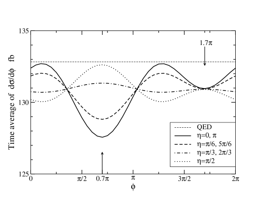
Figure 4: Time averaged azimuthal angle distribution for $\eta=0$, $\pi/6$, $\pi/3$, $\pi/2$, $2\pi/3$, $5\pi/6$, $\pi$. We set the laboratory coordinate system by taking $(\delta,a)=(\pi/4,\pi/4)$. We take $\sqrt{s}=500$GeV and $\theta_{E}=(500{\rm GeV})^{-2}$.

We see from figure 4 that the curves of $\langle{d\sigma}/d\phi\rangle_{T}$ are sensitive to the value of $\eta$ around $\phi\simeq 0.7\pi$ and also almost independent of the value of $\eta$ around $\phi\simeq 1.7\pi$. Furthermore $\langle{d\sigma/d\phi}\rangle_{T}$ is almost flat around $\phi\simeq 1.7\pi$ for any $\eta$.

Those specific angles $0.7\pi$ and $1.7\pi$ can be interpreted as the azimuthal angle of $\overrightarrow{\theta_{ES}}$ and $-\overrightarrow{\theta_{ES}}$ in the laboratory coordinate system. In other words, those are the azimuthal angles of north pole and south pole of the celestial sphere. Since we take $(\delta$, $a)=(\pi/4,$ $\pi/4)$, the azimuthal angle $\phi_{ES}^{N}$ of $\overrightarrow{\theta_{ES}}$ can be derived from (50) as follows

$$\cos\phi_{ES}^{N}=\frac{-c_{\delta}s_{a}}{\sqrt{1-c^{2}_{\delta}c^{2}_{a}}}=-\frac{1}{\sqrt{3}} \sin\phi_{ES}^{N}=\frac{s_{\delta}}{\sqrt{1-c^{2}_{\delta}c^{2}_{a}}}=\sqrt{\frac{\,2\,}{\,3\,}}$$ , (78)

then $\phi_{ES}^{N}\simeq 0.7\pi$ and the azimuthal angle of $-\overrightarrow{\theta_{ES}}$ is given by $\phi_{ES}^{N}+\pi\simeq 1.7\pi$.

We also see from figure 4 that each input $\eta$ and $\pi-\eta$ gives the same distribution of $\langle{d\sigma}/d\phi\rangle_{T}$. This is because the differential cross section of $e^{-}e^{+}\to\gamma\gamma$ is symmetric for $\overrightarrow{\theta_{E}}\leftrightarrow-\overrightarrow{\theta_{E}}$.

We may determine $\eta$, except for two-fold ambiguity for $\eta$ and $\pi-\eta$, by fitting the shape of curve of $\langle{d\sigma/d\phi}\rangle_{T}$, especially around $\phi\simeq\phi_{ES}^{N}=0.7\pi$. Also we may determine $\theta_{E}$ almost independently of $\eta$ by measuring the deficit of $\langle{d\sigma/d\phi}\rangle_{T}$ compared with QED prediction around $\phi\simeq 1.7\pi$.

4.2 Time dependent total cross section

In order to determine $\xi$, we need to trace the apparent time variation of observables due to the earth’s rotation. Since total cross section $\sigma_{obs}$ depends on $\theta_{E}$, $\eta$ and also $\xi$, we may expect that $\theta_{E}$, $\eta$ and $\xi$ could be determined by measuring time variation of $\sigma_{obs}$ precisely, except for the two-fold ambiguity for ($\eta$, $\xi$).

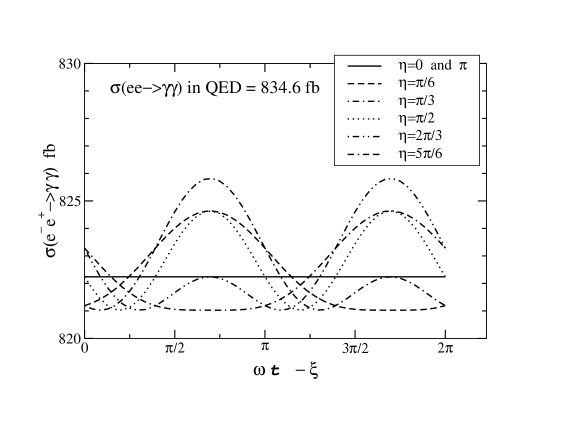
Figure 5: Apparent time variation of total cross section for $\eta=0,\pi/6,\pi/3,\pi/2,2\pi/3,5\pi/6$ and $\pi$. We take $(\delta,a)=(\pi/4,\pi/4)$, $\sqrt{s}=500$GeV and $\theta_{E}=(500$GeV$)^{-2}$.

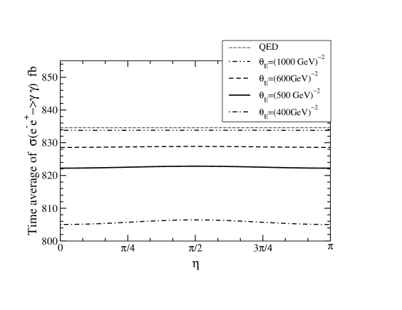
Figure 6: Time averaged total cross section of $e^{-}e^{+}\to\gamma\gamma$ for ${\theta_{E}}=(400{\rm GeV})^{-2},$ $(500{\rm GeV})^{-2},$ $(600{\rm GeV})^{-2}$ and $(1000{\rm GeV})^{-2}$ are shown. Horizontal axis is taken to be angle $\eta$. QED result is also shown. We take $(\delta,a)=(\pi/4,\pi/4)$ and $\sqrt{s}=500$GeV.

Figure 5 shows $\sigma_{obs}$ as a function of $\omega{t}-\xi$ for $\theta_{E}=(500\mbox{GeV})^{-2}$ and for several values of $\eta$. We can see from figure 5 that the shape of curve is sensitive to the $\eta$. If the time variation of total cross section is observed, we could determine both magnitude and direction of $\overrightarrow{\theta_{E}}$ by fitting the NCQED prediction of $\sigma_{obs}$ with the data in three parameters space ($\theta_{E},\eta,\xi$). The magnitude $\theta_{E}$ and the angle $\eta$ may be determined by the fitting of both the magnitude and the shape of curves of $\sigma_{obs}$. The $\xi$ may be determined by the measurement of the phase of time evolution of $\sigma_{obs}$. However, as is mentioned previously, we cannot distinguish ($\eta$, $\xi$) from ($\pi-\eta$, $\pi+\xi$). For example, the graph of $\sigma_{obs}$ for $\eta=\pi/3$ is identical to that for $\eta=2\pi/3$ shifted the phase $\xi$ to $\xi+\pi$.

Although we may determine $\overrightarrow{\theta_{E}}$ by tracing the time variation of the differential cross section of $e^{-}e^{+}\to\gamma\gamma$ instead of total cross section, we can easily imagine that such an experiment needs very large luminosity. This is because we must divide not only the phase space but also the time distribution into many bins, in order to trace the time variation. Therefore, in the determination of $\theta_{E}$, $\eta$ and $\xi$, we had better probe the time variation of total cross section in the early experiments at $e^{-}e^{+}$ linear colliders.

4.3 $\langle{d\sigma/d\phi}\rangle_{T}$ vs. $\sigma_{obs}$

We can see from figures 4 and 5 that $\langle{d\sigma/d\phi}\rangle_{T}$ and $\sigma_{obs}$ show opposite behavior for each input value of $\eta$. For example, when $\eta=0\mbox{ or }\pi$, we may observe large variation of azimuthal angle distribution $\langle{d\sigma/d\phi}\rangle_{T}$. In this case, we find no time variation of $\sigma_{obs}$. On the contrary, when $\eta=\pi/3\mbox{ or }2\pi/3$, since the variation of $\langle{d\sigma/d\phi}\rangle_{T}$ is very small, we may observe the flat distribution in the experiments. In this case, we find large time variation of $\sigma_{obs}$. Therefore we may expect that non-uniform distribution due to NCQED effect should appear in the $\langle{d\sigma/d\phi}\rangle_{T}$ and/or $\sigma_{obs}$ for any value of $\eta$, if ${\theta_{E}}$ is large enough.

4.4 Time averaged total cross section

Finally, we consider what we can measure by the time averaged total cross section $\langle\sigma\rangle_{T}$. Figure 6 shows $\langle\sigma\rangle_{T}$ as a function of $\eta$. It is easy to see that $\langle\sigma\rangle_{T}$ is almost independent of $\eta$. In case of us observing some deficit of $\langle\sigma\rangle_{T}$, we may determine $\theta_{E}$ independently of $\eta$ by measuring $\langle\sigma\rangle_{T}$.

On the other hand, in case of us observing no signal, we may obtain the upper limit on $\theta_{E}$. The $1\sigma$ deviation for total cross section in QED, $\sigma_{QED}$, can be estimated by $\sqrt{{\sigma_{QED}}/{L}}$. For $\sqrt{s}=500$GeV and $\epsilon=0.2$, we have $({28.89}/{\sqrt{L}})$ where $L$ is the luminosity given in fb^-1. In this case, an expected 95%CL upper limit on $\theta_{E}$ is found to be

$$\begin{array}[]{cl}\theta_{E}\mbox{ \raisebox{-4.30554pt}{$\stackrel{{\scriptstyle\textstyle<}}{{\textstyle\sim}}$ }}(600{\rm GeV})^{-2}&\mbox{for $L$=100fb${}^{-1}$}.\end{array}$$ (80)

Furthermore, since $|\sigma_{QED}-\langle\sigma\rangle_{T}|\propto{(s\theta_{E})}^{2}$ for $|s\theta_{E}|<1$, we may estimate 95%CL upper limit on $\theta_{E}$ for arbitrary $L$ from (80) as follows;

$$\theta_{E}\mbox{ \raisebox{-4.30554pt}{$\stackrel{{\scriptstyle\textstyle<}}{{\textstyle\sim}}$ }}(600{\rm GeV})^{-2}\left(\frac{100{\rm fb^{-1}}}{L}\right)^{1/4}.$$ (81)

For example, we find $\theta_{E}\mbox{ \raisebox{-4.30554pt}{$\stackrel{{\scriptstyle\textstyle<}}{{\textstyle\sim}}$ }}(800{\rm GeV})^{-2}$ when $L$=1000fb^-1.

5 Conclusion and Remarks

We have presented phenomenological formulation of the apparent time variation of noncommutativity parameter $\theta_{\mu\nu}$ in the laboratory coordinate system. In our framework, the laboratory coordinate system have been taken to be a familiar coordinates to the collider experiments, and the primary coordinate system fixed to the celestial sphere have been introduced. We have shown the transformation formula between the primary and the laboratory coordinate system, and also shown the expression of $\overrightarrow{\theta_{E}}$ in the laboratory coordinate system. The formulation presented in this paper is applicable to the study of models which predict an intrinsic direction of the space-time[4, 20].

As an example, we have applied our formulation to NCQED and discussed the determination of $\overrightarrow{\theta_{E}}$ at the $e^{-}e^{+}$ linear collider experiments by the process $e^{-}e^{+}\to\gamma\gamma$. The $\overrightarrow{\theta_{E}}$ have been parameterized by $\theta_{E}$, $\eta$ and $\xi$ in the primary coordinate system. We have shown that $\overrightarrow{\theta_{E}}$ may be determined by the detailed study of the time dependent total cross section, though two-fold ambiguity in the parameter space ($\eta$, $\xi$) remains. To determine $\xi$, we need to probe the phase of the time evolution of $\sigma_{obs}$. In case of us observing no signal, probably this is the most realistic case, we may obtain the upper limit on $\theta_{E}$ independently of the direction of $\overrightarrow{\theta_{E}}$.

So far we have considered one experiment with ($\delta$, $a$)=($\pi/4$, $\pi/4$). If there are several detector sites in the $e^{-}e^{+}$ collider experiment and the direction of $e^{-}$ beam in each site is set to be along to the different direction, such as four LEP experiments, then the angular distributions of $e^{-}e^{+}\to\gamma\gamma$ and the time variation of observables should behave differently in each experiment. This is because the direction of $\overrightarrow{\theta_{ES}}$ in the laboratory coordinate system at one detector site differ from that at other detector sites. Therefore we can expect that the combined analysis of several experiments with the different ($\delta$, $a$) play an important role in the attempt to probe the space-time noncommutativity.

Finally, we would like to make some comments on the determination of the magnetic-like component $\overrightarrow{\theta_{B}}$. Since the process $e^{-}e^{+}\to\gamma\gamma$ is independent of $\overrightarrow{\theta_{B}}$, to determine $\overrightarrow{\theta_{B}}$, we must consider other processes relevant to $\overrightarrow{\theta_{B}}$, for example $e^{-}\gamma\to{e^{-}}\gamma$ process which depend on both $\overrightarrow{\theta_{E}}$ and $\overrightarrow{\theta_{B}}$. The process $\gamma\gamma\to\gamma\gamma$ may also be available to determine $\overrightarrow{\theta_{B}}$. By combining the results from those processes, we may determine $\overrightarrow{\theta_{E}}$ and $\overrightarrow{\theta_{B}}$. We postpone the study of this matter to the future studies.

Acknowledgments: The author thanks O. Kamei and A. Sugamoto for reading the manuscript and useful comments, and K. Hagiwara and T. Kawamoto for useful discussion and comments. The author also thanks I. Watanabe for useful comments on the usefulness of $X$ axis defined by the vernal equinox $\Upsilon_{2000.0}$.

References

- [1] H. S. Snyder, Phys. Rev. 71 (1947) 38; Phys. Rev. 72 (1947) 68
- [2] A. Connes, M. R. Douglas and A. Schwarz, J. High Energy Phys. 02 (1998) 0003; N. Seiberg and E. Witten, J. High Energy Phys. 09 (1999) 032
- [3] S. M. Carroll et al., Phys. Rev. Lett. 87 (2001) 141601
- [4] M. Hayakawa, Phys. Lett. B478 (2000) 394
- [5] M. Hayakawa, hep-th/9912167
- [6] J. M. Gracia-Bondía and C. P. Martín, Phys. Lett. B479 (2000) 321; F. Ardalan and N. Sadooghi, Int. J. Mod. Phys. A16 (2001) 3151
- [7] M. M. Sheikh-Jabbari, Phys. Rev. Lett. 84 (2000) 5265
- [8] I. F. Riad and M. M. Sheikh-Jabbari, J. High Energy Phys. 08 (2000) 045; X. J. Wang and M. L. Yan, J. High Energy Phys. 03 (2002) 047
- [9] N. Chair and M. M. Sheikh-Jabbari, Phys. Lett. B504 (2001) 141; M. Haghighat, S. M. Zebarjad and F. Loran, hep-ph/0109105
- [10] M. Chaichian, M. M. Sheikh-Jabbari and A. Tureanu, Phys. Rev. Lett. 86 (2001) 2716
- [11] H. Falomir et al., hep-th/0203260
- [12] J. L. Hewett, F. J. Petriello and T. G. Rizzo, Phys. Rev. D64 (2001) 075012
- [13] H. Arfaei and M. H. Yavartanoo, hep-th0010244; P. Mathews, Phys. Rev. D63 (2001) 075007; S. Godfrey and M. A. Doncheski, hep-ph/0111147; T. G. Rizzo, hep-ph/0203240
- [14] I. Mocioiu, M. Pospelov and R. Roiban, Phys. Lett. B489 (2000) 390; C. E. Carlson, C. D. Carone and R. F. Lebed, Phys. Lett. B518 (2001) 201; S. Baek et al., Phys. Rev. D64 (2001) 056001; I. Hinchliffe and N. Kersting, Phys. Rev. D64 (2001) 116007; H. Grosse and Y. Liao, Phys. Lett. B520 (2001) 63; A. Mazumdar and M. M. Sheikh-Jabbari, Phys. Rev. Lett. 87 (2001) 011301; N. Kersting, Phys. Lett. B527 (2002) 115; W. Behr et al., hep-ph/0202121; E. O. Iltan, hep-ph/0202011; hep-ph/020419; hep-ph/0204332
- [15] H. Grosse and Y. Liao, Phys. Rev. D64 (2001) 115007
- [16] I. Hinchliffe and N. Kersting, hep-ph/0205040
- [17] G. F. Smoot et al., ApJ 371 (1991) L1; G. F. Smoot et al., ApJ 419 (1993) 1
- [18] T. Kawamoto, private communication
- [19] for example, see Particle Data Group: J. Bartels et al., Eur. Phys. J. C15 (2000) 1
- [20] other than NCQED, for example, A. Sugamoto, Prog. Theor. Phys. 107 (2002) 793; G. C. Cho, E. Izumi and A. Sugamoto, hep-ph/0112336