Topological Defect Densities in Type-I Superconducting Phase Transitions

Abstract

We examine the consequences of a cubic term addition to the mean-field potential of Ginzburg-Landau theory to describe first order superconductive phase transitions. Constraints on its existence are obtained from experiment, which are used to assess its impact on topological defect creation. We find no fundamental changes in either the Kibble-Zurek or Hindmarsh-Rajantie predictions.

I Introduction

It is generally believed that the Universe, evolving from the initial Big Bang, underwent a series of symmetry-breaking phase transitions Kibble ; Linde accompanied by the creation of topological defects, frustrations of the unbroken phase within the broken one, induced by continuity of the order parameter values. These defects appear as magnetic monopoles, cosmic strings, domain walls and textures.

Direct experimental tests of these ideas are unfeasible, but transitions described by similar equations occur in experimentally accessible condensed matter systems, and a new trend has unfolded which compares these two systems. This “cosmology in the laboratory” relies on the fact that the dynamics of phase transitions lie in universality classes and the cosmological ones are hence analogous to those of condensed matter. For instance, vortices created in the superfluid phase transitions of ${}^{4}He$ and ${}^{3}He$ have been studied experimentally (see e.g. Ref. Bunkov ; Vollhardt for extensive discussions) following an earlier suggestion in which common features with cosmic strings have been noted Zurek . Similarities between cosmological phase transitions and the isotropic-nematic phase transition in liquid crystals were studied in Refs. Chuang ; Bowick . Analogy with the thermodynamics and transitions in polymer chains was drawn in Ref. Bento .

The case of superconductors is of particular interest as the associated phase transition involves a local gauge symmetry-breaking process.

In superconductors, cosmic strings manifest themselves as flux tubes or vortices. Experiments aimed to observe defect densities in high-$T_{c}$ materials Carmi have lead to contradictory results with respect to the density predicted by the Kibble-Zurek (K-Z) mechanism Kibble . This prediction is however accurate only for global gauge symmetry breaking, a situation where the geodesic rule for phase angle summation is valid. A local gauge treatment by Hindmarsh-Rajantie (H-R) Hindmarsh-Rajantie identifies a new mechanism for defect generation, which leads to a prediction well below the first Carmi-Polturak experiment sensitivity, although the prediction for the second one is in reasonable agreement with observation.

The above experiments were both conducted in type-II materials, which exhibit a second order phase transition. The question naturally arises as to the extent of changes in the defect density predictions for type-I superconductors. This is the motivation for our work.

Distinction between type-I and type-II superconductors is traditionally made through the Ginzburg-Landau (G-L) parameter $\kappa=\lambda/\xi$, the ratio between the magnetic field penetration length, $\lambda$, and the order parameter (scalar field) coherence length, $\xi$. These characteristic length scales are obtained, in the presence of a gauge field $\vec{A}$, from the free energy density

$$F(\Phi)={1\over 2m_{e}}\left|i\hbar\vec{\nabla}\Phi-{e\over c}\vec{A}\Phi\right|^{2}+V(\Phi)+{1\over 2}\vec{\mu}\cdot(\vec{\nabla}\times\vec{A})~{}~{},$$ (1)

where $\vec{\mu}$ is the magnetic moment of the specimen, $m_{e}$ is the electron mass and $\Phi$ is the order parameter. The G-L potential is usually written as Zurek

$$V(\Phi)=\alpha\Phi^{2}+{\beta\over 2}\Phi^{4}~{}~{},$$ (2)

where $\alpha$ is assumed to depend linearly on the temperature, $\alpha=\alpha^{\prime}(t-1)$, $t\equiv T/T_{c}$, $\alpha^{\prime}$ and $\beta$ are constants, and $T_{c}$ is the critical temperature. Thus one obtains

$$\lambda=\sqrt{{m_{e}c^{2}\over 4\pi e^{2}}{\beta\over|\alpha|}}~{}~{},$$ (3)

and

$$\xi={\hbar\over\sqrt{2m_{e}|\alpha|}}~{}~{}.$$ (4)

At $T=0$ the coherence length is given by $\xi_{0}=\hbar/\sqrt{2m_{e}\alpha^{\prime}}$, with $\kappa\sim\sqrt{\beta}$. For $\kappa>1/\sqrt{2}$, the transition is second order, and $\xi_{0}$ is typically less than $\sim 0.04~{}\mu m$; for $\kappa<1/\sqrt{2}$, the transition is first order, with $\xi_{0}$ typically greater than $\sim 0.08~{}\mu m$. In general, both are second order for $H=0$. First order transitions arise from the external field term in Eq. (1) in the event that a characteristic sample dimension is greater than $\lambda$.

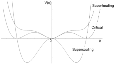
Figure 1: Characteristic Potential curves.

In thermal field theory (TFT) a first order phase transition arises from consideration of 1-loop radiative corrections to a potential of the form of Eq. (2), which introduce a barrier between minima through a cubic scalar field term, as

$$V(\Phi)=\alpha\Phi^{2}-\gamma|\Phi|^{3}+{\beta\over 2}\Phi^{4}~{}~{},$$ (5)

where $\gamma(T)=(\sqrt{2}/4\pi)e^{3}T$ Hindmarsh . As in the previous case, $\beta$ is constant and $\alpha=\alpha^{\prime}(t-1)$ is linear with temperature.

A similar $-\gamma|\Phi|^{3}$ term however, arises in considerations of gauge field fluctuations in the normal-to-superconductor phase transition Halperin ; Hove , with

$$\gamma=8\mu_{0}{e\over\hbar c}\sqrt{\pi\mu_{0}}T_{c}~{}~{},$$ (6)

resulting in a first order phase transition for all values of $\kappa$. Crossovers between first and second order transitions arise in considerations of thermal fluctuations Hove , as also in nonlocal BCS treatments Brandt .

With this is mind, we adopt a potential of the form of Eq. (5) and explore constraints on $\gamma(T)$ from experiment. The results are compared with TFT 1-loop radiative corrections. Comparison with the results of Ref. Halperin , which deals with temperatures close to $T_{c}$, is attained in the limit $t\rightarrow 1$.

These results are then used to analyze the impact of the cubic term on the K-Z and the H-R predictions for type-I superconductors, namely on the models themselves and on a possible nucleation suppression due to the slowing down of the transition induced by the potential barrier.

II Temperature sensitivity bound

A first-order superconductive phase transition manifests supercritical fields under variation of the temperature, as shown in Figure 1. The superheating curve is given by the condition ${dV\over d\Phi}={d^{2}V\over d\Phi^{2}}=0$, for a certain value of $\Phi\neq 0$. This yelds $\alpha=9\gamma^{2}/16\beta$.

In contrast, the supercooling curve is given by the condition ${d^{2}V(\Phi)\over d\Phi^{2}}=0$ for $\Phi=0$, corresponding to $\alpha=0$. The unobservable critical curve is given by the condition $V(0)=V(\Phi_{c})$ and ${dV(\Phi_{c})\over d\Phi}=0$, where $\Phi_{c}$ is the non-vanishing minimum of the potential. This corresponds to $\alpha=\gamma^{2}/2\beta$.

Introducing the linear dependencies $\alpha=\alpha^{\prime}(t-1)$ and $\gamma(t)=\delta~{}t$, we obtain for the superheating curve

$$\alpha^{\prime}(t-1)={9\over 16}{\delta^{2}\over\beta}t^{2}~{}~{},$$ (7)

and hence

$$t_{sh}={2\over 1+\sqrt{1-{9\over 4}{\delta^{2}\over\alpha^{\prime}\beta}}}\sim 1+{9\over 16}{\delta^{2}\over\alpha^{\prime}\beta}~{}~{}.$$ (8)

The superheating curve converges to a zero-field shift in temperature from $T_{c}$ by $(9\delta^{2}/16\alpha^{\prime}\beta)T_{c}$. This shift is undetected at the current experimental temperature sensitivity of $\Delta t_{exp}\sim 10^{-3}$ tempmeas . Therefore, a bound for the slope of $\gamma$ is

$${9\over 16}{\delta^{2}\over\alpha^{\prime}\beta}<\Delta t_{exp}~{}~{}.$$ (9)

The supercooling transition occurs at $t=1$, the critical temperature, since it is determined solely by $\alpha=0$ (this neglects a small correction to $\alpha$, as given by Ref. Halperin ).

III Superheating perturbation bound

Table 1: Critical properties of $Sn$ and $Al$

Material	$T_{c}~{}(K)$	$H_{c}(0)~{}(G)$	$\xi_{0}~{}(\mu m)$	$\lambda~{}(nm)$
Sn	$3.7$	$309$	$0.23$	$34$
Al	$1.2$	$105$	$1.6$	$16$

Measurements of the supercritical fields have commonly been performed on microspheres of type-I materials as a means of determining $\kappa$. Table 1 indicates the critical properties of two, Sn and Al. The existence of a cubic term should also be manifest in the presence of a magnetic field. To assess its influence, we repeat Ref. Ginzburg calculations, including the cubic term in the potential. For a small superconducting sphere of radius $a$, the magnetic moment is given by Ginzburg

$${\mu\over V}=-3\left[1-{3\lambda\over a\Phi_{0}}coth{a\Phi_{0}\over\lambda}+{3\lambda^{2}\over a^{2}\Phi_{0}^{2}}\right]{H\over 8\pi}~{}~{},$$ (10)

where $\Phi_{0}\equiv\Phi/\Phi_{\infty}$ and $\Phi_{\infty}^{2}\equiv m_{e}c^{2}/4\pi e^{2}\lambda^{2}$.

After a somewhat lengthy computation (see Appendix), the reduced superheating field, $h_{sh}\equiv H_{sh}/H_{c}$, is given by

$$h_{sh}=\left(1+{4\over\sqrt[4]{15}}\gamma_{G}\right)h_{sh}^{0}~{}~{},$$ (11)

where $\gamma_{G}\equiv 3\gamma/2\sqrt{|\alpha|\beta}$ is a dimensionless parameter, and $h_{sh}^{0}$ is the “unperturbed” ($\gamma=0$) superheating field.

Generally, such measurements have been obtained with colloids, and the size distributions of the microspheres data1 ; data2 ; data4 ; data5 ; data6 provides a statistical error which renders a direct fit of $\gamma_{G}$ from $h_{sh}(t)$ data unfeasible. Although the measurement reported in Ref. data3 was conducted using single microspheres, non-local and impurity effects lead to a large theoretical uncertainty in

$$h_{sh}^{0}(t)={1\over\sqrt{\kappa\sqrt{2}}}h_{c}^{0}(0)(1-t^{2})~{}~{},$$ (12)

where $h_{c}^{0}(0)=H_{c}(0)/H_{c}(t)$, which is itself an approximation valid only close to $T_{c}$ hcorr .

Since the supercooling field implies the evaluation of a second derivative at the origin, it can be easily seen that the presence of a cubic term has no effect:

$${d^{2}\over d\Phi^{2}}(\gamma_{G}\Phi^{3})=6\gamma_{G}\Phi\rightarrow 0~{}~{}.$$ (13)

The effect of $\gamma$ (through $\gamma_{G}$) on the superheating field must be small, otherwise it would have been already detected; therefore, we must have $\gamma_{G}\ll 1$, which is not valid for relative temperatures in the range

$$1-{9\over 4}{\delta^{2}\over\alpha^{\prime}\beta}<t<1~{}~{}.$$ (14)

For this interval to be vanishingly small,

$${9\over 4}{\delta^{2}\over\alpha^{\prime}\beta}\ll 1~{}~{}.$$ (15)

This is a weaker bound than the one of Eq. (9).

For Al and Sn with maximum critical fields of order $10^{2}~{}G$, the shift between $h_{sh}$ and $h_{sh}^{0}$ is less than $10^{-2}~{}G$, well below the sensitivity of measurements data1 ; data2 ; data3 ; data4 ; data5 ; data6 . For this reason, we simply drop the bound of Eq. (15) and consider only the one of Eq. (9). Conversely, a breakdown of the perturbation expansion of the superheating reduced field would imply a superheating temperature shifted to $t_{sh}=1.6$. Also notice that no “spikes” should be seen in the $H-T$ superheating curve for values of $t$ in the “exclusion” interval as the field values are quite small there.

Table 2: Derived quantities and bounds for $\delta$

Material	Sn	Al
$\alpha^{\prime}~{}(J)$	$1.15\times 10^{-25}$	$2.38\times 10^{-27}$
$\beta~{}(J.m^{3})$	$4.72\times 10^{-54}$	$2.16\times 10^{-56}$
$\alpha^{\prime}~{}(eV^{2})$	$3.61\times 10^{-1}$	$7.45\times 10^{-3}$
$\beta$	$9.45\times 10^{-4}$	$4.32\times 10^{-6}$

bound	$t_{sh}$ shift	$\delta(eV)$	$t_{sh}$ shift	$\delta(eV)$
$h_{sh}$	$0.25$	$1.23\times 10^{-2}$	$0.25$	$1.20\times 10^{-4}$
$\Delta T_{exp}$	$10^{-3}$	$7.78\times 10^{-4}$	$10^{-3}$	$7.57\times 10^{-6}$
Ref. Halperin	$5.19\times 10^{-9}$	$1.77\times 10^{-6}$	$2.32\times 10^{-6}$	$3.64\times 10^{-7}$
TFT	$2.92\times 10^{-9}$	$1.33\times 10^{-6}$	$3.24\times 10^{-6}$	$4.31\times 10^{-7}$

Table 2 provides a comparison of the bounds on $\delta$ with the prediction of Ref. Halperin . The analogy between cosmology and condensed matter prompts for comparison with the TFT cubic term also. To do this, we compute the associated slope of $\gamma(t)$ from $\gamma(T)=(\sqrt{2}/4\pi)e^{3}T$, obtaining $\delta=(\sqrt{2}/4\pi)e^{3}T_{c}$. Obviously, although the prediction is material independent, its formulation in terms of a reduced temperature is not.

Note that the dimensionality of $\gamma$ here is changed with respect to the free energy potential of Eq. (5), through a convenient $m_{e}$ factor – this is because the dimension of the scalar field in G-L theory is $[\Phi^{2}]=L^{-3}$, its square representing a density, while in field theory $[\Phi]=L^{-1}$. The electron mass determines the conversion as it is absent from the kinetic term of the Lagrangean density of field theory, $\partial_{\mu}\Phi\partial^{\mu}\Phi$, while present in the corresponding condensed matter free energy term, $(\hbar^{2}/2m_{e})\nabla^{2}\Phi$ (or, equivalently, in the coherence length: $\xi^{2}_{FT}=1/\alpha^{\prime}$ vs. $\xi^{2}_{cm}=\hbar^{2}/2m_{e}\alpha^{\prime}$).

Table 2 also includes the quantities $\alpha^{\prime}$ and $\beta$, both in SI and natural units. As explained above, conversion is not direct, but achieved through the multiplicative factor $m_{e}$.

The results in Table 2 include the cubic term predicted by Ref. Halperin . In the absence of an applied magnetic field, each momentum-fluctuation of the gauge field $\vec{A}$ has an expectation value given by the equipartition theorem. When suitably integrated over the momentum space (with a cutoff $\Lambda$ of the order of $\xi_{0}^{-1}$),

$$\langle A^{2}\rangle_{\Phi}=4{\mu_{0}\over\pi}\Lambda T_{c}-8\mu_{0}{e\over\hbar c}\sqrt{\pi\mu_{0}}T_{c}|\Phi|~{}~{}.$$ (16)

Since $A^{2}$ couples to $\Phi^{2}$ in Eq. (1), this translates into an unimportant correction to the scalar field mass, plus a negative cubic term, given by $-8\mu_{0}(e/\hbar c)\sqrt{\pi\mu_{0}}T_{c}|\Phi|^{3}~{}$. This term implies a shift in the superheating temperature (at zero field), of

$$\Delta_{T}=7.25\times 10^{-12}T_{c}^{3}H_{c}(0)^{2}\xi_{0}^{6}~{}~{},$$ (17)

with $H_{c}(0)$ in Gauss and $\xi_{0}$ in $\mu m$.

This shift lies beyond experimental accessibility, since it requires a temperature sensitivity of $10^{-6}K$ (for Al; $10^{-9}K$ for Sn). However, such an experiment might be performed with Al, using state of the art relative temperature measurement techniques.

Surprisingly, for both materials the slopes of $\gamma$ predicted by TFT and Ref. Halperin have similar magnitudes, $\sim 10^{-7}eV$. This is an indication of the analogous underlying mechanisms behind them: the thermal averaging of the gauge field in condensed matter can be thought of as equivalent to finite temperature vacuum polarization in high energy physics (expressed by the renormalization of 1-loop Feynmann diagrams).

IV Topological defect formation

Let us now discuss some possible implications of the inclusion of the cubic term in the mean-field potential. Since temperature sensitivity measurements constrain $\gamma_{G}<10^{-2}$, we always assume $\gamma^{2}\ll\alpha\beta$.

The K-Z mechanism predicts a density of topological defects (vortices), $n\simeq\xi^{-2}_{0}({\tau_{0}/\tau_{q}})^{\nu}$, where $\tau_{0}=\pi\hbar/16k_{B}T_{c}$ is the characteristic time scale, given by the Gorkov equation, $\tau_{q}$ is the quench time, and $\nu$ is a critical exponent. Moreover, it rests upon the assumption that there is a single topological defect per $\xi^{2}_{0}$ area and, therefore, one must look for changes induced in this quantity. However, since the characteristic scales of the problem are obtained via linearization of the G-L equations, close to $T_{c}$ and when the order parameter is small, we see no changes in this prediction.

On the other hand, for a thin slab of of width $L_{z}$, the H-R mechanism predicts a defect density of the order $n\simeq(e/2\pi)T^{1/2}L_{z}^{-1/2}\hat{\xi}^{-1}$, where $\hat{\xi}\sim 2\pi/\hat{k}$ is the domain size immediately after the transition. This quantity is related to the highest wavenumber $\hat{k}$ to fall out of equilibrium and is obtained from the adiabaticity relation

$$\left|{d\omega(k)\over dt}\right|=\omega^{2}(k)~{}~{},$$ (18)

for a given dispersion relation $\omega(k)$. In the underdamped case, $\omega(k)=\sqrt{k^{2}+m_{\gamma}^{2}}~{}$, with a photon mass given by $m_{\gamma}^{2}=2e^{2}|\Phi|^{2}=-2e^{2}\alpha/\beta~{}$. Thus we obtain $\hat{k}\sim\sqrt[3]{\alpha^{\prime}e^{2}/\beta\tau_{q}}$, and hence $n\propto\tau_{q}^{-1/3}~{}$. Here, the introduction of a cubic term in the potential will change the photon mass, as the true vacuum shifts to

$$\Phi={-3\gamma+\sqrt{-16\alpha\beta+9\gamma^{2}}\over 4\beta}~{}~{}.$$ (19)

However, since $\gamma_{G}\equiv 3\gamma/2\sqrt{|\alpha|\beta}\ll 1$, the effect of the cubic term is too small to significantly change the H-R result.

Another effect related to metastability concerns the non-vanishing probability of the order parameter to quantum tunnel from the the symmetric (false) vacuum towards the non-symmetric vacuum. Following Refs. Coleman ; Linde2 , the rate of transition per unit volume and time to the true vacua is given, in the thin wall approximation, by

$${\Gamma\over V\Delta t}=T^{4}\left({S_{3}\over 2\pi~{}T}\right)^{3/2}e^{-S_{3}/T}~{}~{},$$ (20)

where

$$S_{3}(T)={2\pi\over 81}{1\over\beta^{7}\sqrt{\beta}}{\gamma^{9}(T)\over\epsilon^{2}(T)}$$ (21)

is the Euclidean action, and $\epsilon(T)$ is the “depth” of the true vacuum.

The thin wall approximation is valid whenever the barrier’s height is much greater than $\epsilon$. This is true when $\gamma$ is comparable to the other parameters, namely when $\gamma_{G}\sim 1$. For eventually smaller values of $\gamma$, like those predicted by TFT and Ref. Halperin , the approximation fails. In fact, we have shown that the current temperature sensitivity of $10^{-3}K$ only allows values of $\gamma_{G}$ smaller than $10^{-2}$. Therefore, we must conclude that the barrier’s height is not comparable to the true vacuum’s depth, and the field should always tunnel through it (i.e. with a probability close to unity). Because of this, there is no concern that defects may not have time to nucleate within the resolution time of the measuring device, as would happen if the potential barrier were high and diminished too slowly.

V Conclusions

In this work we have examined a possible description of a type-I superconductive phase transition by introducing a cubic term in the G-L mean-field potential, inspired by a gauge field thermal averaging Halperin , and also by analogy with TFT.

Our analysis of the bounds derived from the superheating field and temperature constraints clearly show that the contribution of any cubic term is small compared to other parameters in the G-L potential. Thus the following conclusions can be drawn: First, the superheating temperature shift induced by a cubic term, derived either from Ref. Halperin or from TFT, increases with decreasing G-L parameter $\kappa$ ($\Delta t_{sh}(Sn)\sim 10^{-9}$; $\Delta t_{sh}(Al)\sim 10^{-6}$). This suggests that future experiments to search for a TFT cubic term should be conducted with extreme ($\kappa\ll 1$) type-I materials, for example $\alpha$-tungsten, with $T_{c}=15.4\pm 0.5~{}mK$, $H_{c}=1.15\pm 0.03~{}G$. Similarly, the shift in the supercritical field might be reinvestigated using a DC SQUID, which currently possess a sensitivity of $10^{-5}\phi_{0}/\sqrt{Hz}$, or $10^{-6}G$ over a 10 $\mu$m grain diameter.

Furthermore, the impact of any cubic term on the defect density predictions of K-Z Kibble ; Zurek or H-R Hindmarsh-Rajantie is negligible, with no suppression or slowing down of defect production because the potential barrier due to $\gamma$ is not sufficient to prevent nucleation.

These considerations suggest that, all else being equal, experiments to detect topological defect formation in type-I superconductors would observe a reduction of the predicted H-R defect densities by $10-100$ depending on choice of material. Recent calculations Shapiro however suggest that the defect structure formed in type-I materials survives significantly longer than in type-II. Given that the type-I estimate is of order $10^{-4}$ seconds, it seems possible that the disadvantage in $\xi$ might be compensated by simple measurability.

VI Appendix

Including the presence of a magnetic field with a $\Phi$ dependent magnetic moment, the conditions for the reduced superheating field $h_{sh}\equiv H_{sh}/H_{c}$ are

(i) minimum

$$h_{sh}^{2}={8\over 9}\left[{\Phi_{0}^{2}~{}(1+\gamma_{G}\Phi_{0}-\Phi_{0}^{2})~{}sinh^{2}(x_{0})\over 1+{sinh(2x_{0})\over 2x_{0}}-{2sinh^{2}(x_{0})\over x_{0}^{2}}}\right]$$

(ii) inflexion point

$$h_{sh}^{2}={4\over 9}\left[{\Phi_{0}^{2}~{}(1+2\gamma_{G}\Phi_{0}-3\Phi_{0}^{2})~{}x_{0}^{2}sinh^{2}(x_{0})\over 3~{}sinh^{2}(x_{0})-x_{0}^{3}~{}coth(x_{0})-x_{0}^{2}-{1\over 2}x_{0}~{}sinh(2x_{0})}\right]$$

where $x_{0}\equiv\Phi_{0}a/\lambda$.

Since the diameter $a$ is much larger than the penetration depth $\lambda$, we can take the limit $x_{0}\rightarrow\infty$. The above conditions become

$$h_{sh}^{2}={8\over 9}\Phi_{0}^{3}~{}(1+\gamma_{G}\Phi_{0}-\Phi_{0}^{2})~{}{a\over\lambda}$$

and

$$h_{sh}^{2}={4\over 9}\Phi_{0}^{3}~{}(1+2\gamma_{G}\Phi_{0}-3\Phi_{0}^{2})~{}{a\over\lambda}~{}~{}.$$

Solving for $\Phi_{0}$ we get

$$2(1+\gamma_{G}\Phi_{0}-\Phi_{0}^{2})=-(1+2\gamma_{G}\Phi_{0}-3\Phi_{0}^{2})$$

which implies that

$$\Phi_{0}=\sqrt{{3\over 5}+{4\over 25}\gamma_{G}^{2}}+{2\over 5}\gamma_{G}\simeq\sqrt{3\over 5}+{2\over 5}\gamma_{G}~{}~{}.$$

Substituting in the first expression, we obtain

$$h_{sh}^{2}={8\over 9}(\sqrt{3\over 5}+{2\over 5}\gamma_{G})^{3}(1+\gamma_{G}(\sqrt{3\over 5}+{2\over 5}\gamma_{G})-(\sqrt{3\over 5}+{2\over 5}\gamma_{G})^{2}){a\over\lambda}$$

which, to first order in $\gamma_{G}$, becomes

$$h_{sh}={4\over 5\sqrt[4]{15}}\left(1+{4\over\sqrt[4]{15}}\gamma_{G}\right)\sqrt[4]{a\over\lambda}~{}~{},$$

which is the result Eq. (11) as

$$h_{sh}^{0}={4\over 5\sqrt[4]{15}}\sqrt[4]{a\over\lambda}~{}~{}.$$

- (1) T.W.B. Kibble, J. Phys. A9 (1976) 1387; Phys. Rev. 67 (1980) 183; T.W.B. Kibble, M. Hindmarsh, Rep. Prog. Phys. 58 (1995) 477.
- (2) A.D. Linde, Rep. Prog. Phys. 42 (1979) 294 and references therein.
- (3) “Topological Defects and the Non-Equilibrium Dynamics of Symmetry Breaking Phase Transitions”, Y.M. Bunkov, H, Godfrin, Eds. (NATO Science Serious - Vol. 549, 1999).
- (4) D. Vollhardt, P. Wolfle, Acta Phys. Pol. B31 (2000) 2837.
- (5) W.H. Zurek, Physics Reports 276 (1996) 177.
- (6) M. Bowick, L. Chandar, E. Schiff, A. Srivastava, Science 263 (1994) 943.
- (7) I. Chuang, N. Turok, B. Yurke, Phys. Rev. Lett. 66 (1991) 2472.
- (8) M.C. Bento, O. Bertolami, Phys. Lett. A193 (1994) 31.
- (9) R. Carmi, E. Polturak, Phys. Rev. B60 (1999) 7595; R. Carmi, G. Koren, E. Polturak, Phys. Rev. Lett. 84 (1999) 4966.
- (10) M. Hindmarsh, A. Rajantie, Phys. Rev. Lett. 85 (2000) 4660; A. Rajantie, Int. J. Mod. Phys. A17 (2002) 1.
- (11) M. Hindmarsh, A. Davis, R. Brandenberger, Phys. Rev. D49 (1994) 1944.
- (12) B.I. Halperin, T.C. Lubensky, S. Ma, Phys. Rev. Lett. 32 (1974) 292.
- (13) J. Hove, S. Mo, A. Sudbø, Phys. Rev. B66 (2002) 064524.
- (14) E.H. Brandt, Physica C369 (2002) 10.
- (15) “Superconductive Applications: SQUIDS and Machines”, B.B. Schwartz, S. Foner, Eds. (Plenum, New York, 1977); “Low Temperature Techniques”, A.C. Rose-Innes (English Universities Press, London, 1964).
- (16) F.W. Smith, A. Baratoff, M. Cardona, Phys. Kondens. Materie 12 (1970) 145.
- (17) A. Larrea et. al., Nucl. Inst. Meth. A317 (1992) 541.
- (18) J. Feder, D. McLachlan, Phys. Rev. 177 (1968) 763.
- (19) F. de la Cruz, M.D. Maloney, M. Cardona, in Proc. Conf. on Science of Superconductivity, Stanford (1969) 749.
- (20) I.O. Kulik, Soviet. Phys. JETP 28 (1969) 461.
- (21) C.R. Hu, V. Korenman, Phys. Rev. 178 (1969) 685; Phys. Rev. 185 (1969) 672.
- (22) V.L. Ginzburg, Soviet. Phys. JETP 34 (1958) 113.
- (23) Experimentally, , where depends on whether the superconductor is strong- or weak-coupled: B. Muhlschlegel, Z. Phys. 155 (1959) 313; moreover, the leading is only the first term in a general expansion of in : A.J. Dolgert, S.J. DiBartolo, A.T. Dorsey, Phys. Rev. B53 (1996) 5650.
- (24) S. Coleman, Phys. Rev. D15 (1977) 2929.
- (25) A.D. Linde, Phys. Lett. B100 (1981) 37; Nucl. Phys. B216 (1983) 421.
- (26) B.Y. Shapiro, I. Shapiro, M. Ghinovker, Jour. Low Temp. Phys. 116 (1999) 9.