June, 2002

OU-HET 414

hep-ph/0206207

Exploring the neutrino mass matrix at $M_{R}$ scale

Takahiro Miura, Tetsuo Shindou and Eiichi Takasugi

Department of Physics, Osaka University
Toyonaka, Osaka 560-0043, Japan

Abstract

We discuss the neutrino mass matrix which predicts zero or small values of $|V_{13}|$ in the MSSM and found the inequality, $\sin^{2}2\theta_{12}\leq\sin^{2}2\theta_{\odot}$, where $\sin^{2}2\theta_{12}$ is the mixing angle at $M_{R}$ scale and $\sin^{2}2\theta_{\odot}$ is the value determined by the solar neutrino oscillation. This constraint says that the model which predicts a larger value of $\tan^{2}\theta_{12}$ at $M_{R}$ than the experimental value is excluded. In particular, the bi-maximal mixing scheme at $M_{R}$ scale is excluded, from the experimental value $\tan^{2}\theta_{\odot}<1$. In this model, $|V_{13}|$ and a Dirac phase at $m_{Z}$ which are induced radiatively may not be small.

1 Introduction

The SuperKamiokande data has discovered the neutrino mixing between $\nu_{\mu}$ and $\nu_{\tau}$ from the atmospheric dataSuperK-Atm . Now the SNO dataSNO-Solar together with SuperKamiokande dataSK-Solar have solved the solar neutrino puzzle and pinpointed a solution among four solutions. That is, its origin is mainly due to the mixing between the $\nu_{e}$ and $\nu_{\mu}$ and the LMA solution is the most probable one. They are summarized as

$$\tan^{2}\theta_{\odot}\simeq 0.34\;, \Delta m_{\odot}^{2}\simeq 5\times 10^{-5}\;{\rm eV}^{2}\;,$$

$$\sin^{2}2\theta_{\rm atm}\simeq 1\;, \Delta m_{\rm atm}^{2}\simeq 3\times 10^{-3}\;{\rm eV}^{2}\;,$$ (1)

where $\theta_{\odot}$ and $\theta_{\rm atm}$ are mixing angles which appear in the solar and atmospheric neutrino oscillations, and in effect are mixing angles between the 1st and the 2nd and between the 2nd and the 3rd mass eigenstates, respectively. $\Delta m_{\odot}^{2}$ and $\Delta m_{\rm atm}^{2}$ are the squared mass differences defined by $\Delta m_{\odot}^{2}=m_{2}^{2}-m_{1}^{2}$ and $\Delta m_{\rm atm}^{2}=|m_{3}^{2}-m_{2}^{2}|$, where $m_{i}$ is the mass of the $i$-th mass eigenstate of neutrinos. Usually, the sign convention, $\Delta m_{\odot}^{2}=m_{2}^{2}-m_{1}^{2}>0$ is taken, in which case the result from the SNO-SuperKamiolande dataSNO-Solar ; SK-Solar favors the normal side, $\tan^{2}\theta_{\odot}<1$, and disfavors the dark side, $\tan^{2}\theta_{\odot}>1$ Darkside . Another important information from the CHOOZ dataCHOOZ gives a severe upper limit for $|V_{13}|$

$$|V_{13}|<0.16\;,$$ (2)

where $V_{13}$ is the element of the MNS neutrino mixing matrixMaki:mu representing the mixing between the 1st and the 3rd mass eigenstates. If we combine these information, the neutrino mixing matrix is approximately written by

$$V=\begin{pmatrix}c_{\odot}&-s_{\odot}&0\cr s_{\odot}c_{\rm atm}&c_{\odot}c_{\rm atm}&-s_{\rm atm}\cr s_{\odot}s_{\rm atm}&c_{\odot}s_{\rm atm}&c_{\rm atm}\cr\end{pmatrix}\begin{pmatrix}1&&\cr&e^{i\alpha_{M}}&\cr&&e^{i\beta_{M}}\cr\end{pmatrix}\;,$$ (3)

where we included two Majorana CP violation phasesBilenky:1980cx ; DBD-Majo ; SV in the mixing matrix which play an important role for the neutrinoless double beta decayDBD-Majo .

Among the above experimental information, the most mysterious point is the puzzle why $|V_{13}|$ is so small in comparison with other mixing angles, $\theta_{\odot}$ and $\theta_{\rm atm}$. If it is really small, we have to find out the reason for it. For a small quantity at the low energy scale, the naturalness usually asserts that it is zero at the higher energy scale, because it is quite hard to reproduce such a small quantity at the low energy scale.

In this paper, we consider a possibility that $|V_{13}|=0$ at the energy scale where the left-handed neutrino mass is induced by the see-saw mechanism. There are many advantages to consider this possibility. (1) The small value of $|V_{13}|$ is naturally explained because it is induced by the radiative correction. (2) This scenario may be realized in some theoretical models at $M_{R}$ scaleBiMax ; Demo ; TriMax ; Fukuura:1999ze . (3) The Dirac CP violation phase is induced by the radiative correction.

Now, we consider the neutrino mass matrix which predicts $|V_{13}|=0$ at $M_{R}$ scale, in the diagonal basis of the charged lepton mass matrix. This mass matrix contains only seven parameters, three neutrino masses, two mixing angles and two Majorana CP violation phases, and thus there is no Dirac CP violation phase at $M_{R}$ scale. This may gives an possibility that the Dirac CP violation phase which appears in the neutrino oscillation may be related to Majorana CP violation phases, which may be related in the leptogenesis, since in our model, two Majorana phases are associated with phases of neutrino masses and they may well have some relation with phases from the heavy right-handed Majorana mass matrix.

This paper is organized as follows: In Section 2, we explain our model and the framework of neutrino mass matrix. The radiative correction is taken into account and the mass matrix is diagonalized analytically to connect the parameters at $M_{R}$ scale and the present experimental scale, $m_{Z}$. In Section 3, the general feature of our result is explained and the predictions are given. In Section 4, by using analytic result, numerical analysis is made on the induced size of $|V_{13}|$, the Dirac CP violation phase, $\delta$, and the effective mass of the neutrinoless double beta decay. The discussion on the absolute size of neutrino mass is given. Summary and discussions are given in Section 5.

2 The model

We consider a class of left-handed neutrino mass matrices which gives $V_{13}=0$, where $V$ is the neutrino mixing matrix. We assume that this mass matrix is derived by the see-saw mechanism according to the SUSY GUT scenario at the right-handed neutrino mass, $M_{R}$ scale and evolves following the renormalization equation for MSSM to the Z boson mass scale, $m_{Z}$. In this model, $V_{13}$ at $m_{Z}$ scale is induced by radiative correction. We examine the size of $V_{13}$, the Dirac CP violation phase, $\delta$, Majorana CP violation phases, $\alpha_{M}$ and $\beta_{M}$, and the effective mass of the neutrinoless double beta decay, $\langle m_{\nu}\rangle$.

(a) The mass matrix at $M_{R}$

The mass matrix which gives $V_{13}=0$ is generally expressed in the diagonal basis of the charged lepton mass matrix as

$$m_{\nu}(M_{R})=OD_{\nu}O^{T}\;,$$ (4)

where

$$D_{\nu}={\rm diag}(M_{1},M_{2}e^{i\alpha_{0}},M_{3}e^{i\beta_{0}})\;,$$ (5)

with Majorana phases, $\alpha_{0}$ and $\beta_{0}$. $O$ is the mixing matrix at $M_{R}$ scale and is given by

$$O=\begin{pmatrix}1&0&0\cr 0&c_{23}&-s_{23}\cr 0&s_{23}&c_{23}\cr\end{pmatrix}\begin{pmatrix}c_{12}&-s_{12}&0\cr s_{12}&c_{12}&0\cr 0&0&1\cr\end{pmatrix}\;.$$ (6)

with $c_{ij}=\cos\theta_{ij}$ and $s_{ij}=\sin\theta_{ij}$. In the following, we use $\theta_{ij}$ only as an angle at $M_{R}$ scale.

(b) The neutrino mass matrix at $m_{Z}$

In MSSM, the neutrino mass matrix at $m_{Z}$ is given byRGE-formula

$$m_{\nu}(m_{Z})={\rm diag}(1,1,\alpha)OD_{\nu}O^{T}{\rm diag}(1,1,\alpha)\;,$$ (7)

where $\alpha$ is defined by

$$\alpha\equiv 1-\epsilon=1/\sqrt{I_{\tau}}=\Biggl{(}\frac{m_{Z}}{M_{R}}\Biggr{)}^{\frac{1}{8\pi^{2}}(1+\tan^{2}\beta)(m_{\tau}/v)^{2}}<1\;.$$ (8)

Here $m_{\tau}$ is the $\tau$ lepton mass, $v^{2}=v^{2}_{u}+v^{2}_{d}$ and $\tan\beta=v_{u}/v_{d}$ with $v_{i}$ being the vacuum expectation value of MSSM Higgs doublet $\langle H_{i}\rangle(i=u,d)$.

In order to estimate $\epsilon$, we assume the right-handed mass scale, $M_{R}$ and the region of $\tan\beta$ as

$$M_{\rm R}=10^{13}({\rm GeV})\;,\qquad 2<\tan\beta<50\;.$$ (9)

Then, with $m_{Z}=91.187({\rm GeV})$, $m_{\tau}=1.777({\rm GeV})$ and $v=245.4({\rm GeV})$, we find

$$8\times 10^{-4}<\epsilon<5\times 10^{-2}\;.$$ (10)

(c) Masses and the mixing matrix at $m_{Z}$

The effect of the radiative correction to neutrino mass matrix has been discussed by many authorsRGE-formula ; Stability ; RGEwithMaj and the following is known. (1) The mixing angles are stable for the case of the hierarchical or the inverted-hierarchical neutrino mass scheme, $m_{1}\ll m_{2}\ll m_{3}$ or $m_{3}\ll m_{1}\ll m_{2}$. (2) The instability occurs for $m_{1}\simeq m_{2}$. (3) The Majorana phases in neutrino masses may play an important roleRGEwithMaj .

Since the stable case is well analyzed, we focus on the unstable case. That is, we consider the following mass relation holds at $M_{R}$ scale,

$$M_{1}\simeq M_{2}\;,\;0<\Delta_{21}\ll|\Delta_{31}|\;,$$

$$0<\Delta_{21}\ll M_{1}^{2}\;,\;\epsilon M_{1}^{2}\simeq\epsilon M_{2}^{2}\ll|\Delta_{31}|\;,$$ (11)

where $\Delta_{21}=M_{2}^{2}-M_{1}^{2}$, $\Delta_{31}=M_{3}^{2}-M_{1}^{2}$ and we chose the convention, $\Delta_{21}>0$. The diagonalization of the neutrino mass matrix is made analytically and the derivation is given in Appendix.

In the following, we summarize the result derived in Appendix. As for neutrino masses themselves, corrections are small and of order $\epsilon M_{i}$, because we are considering the situation where $M_{1}^{2}\simeq M_{2}^{2}\gg\Delta_{21}\sim\epsilon M_{2}^{2}$. Thus, neutrino masses at $M_{R}$ and $m_{Z}$ can be considered to be the same.

$$m_{i}\simeq M_{i}\;.$$ (12)

The radiative correction gives effect to the mass difference between $m_{1}$ and $m_{2}$,

$$\Delta m_{\odot}^{2}=m_{2}^{2}-m_{1}^{2}=\frac{\Delta_{21}-4\epsilon m_{1}^{2}s_{\rm atm}^{2}\cos 2\theta_{12}}{\cos 2\theta}>0\;,$$ (13)

while the mass difference between the 2nd and the 3rd receives only a negligible effect, so that

$$\Delta m_{\rm atm}^{2}=m_{3}^{2}-m_{2}^{2}\simeq m_{3}^{2}-m_{1}^{2}\simeq\Delta_{31}\;.$$ (14)

In the above, we required $\Delta m_{\odot}^{2}>0$ in accordance with the common experimental analysis which gives $\tan^{2}\theta_{\odot}=0.34<1$. As for mixing angles, the radiative correction does not give any effect to the mixing between the 2nd and the 3rd mass eigenstates either. That is,

$$\theta_{\rm atm}=\theta_{23}\;.$$ (15)

Thus, in the following, we use $m_{i}$ for $M_{i}$ except for the discussion of the mass difference and $\theta_{\rm atm}$ for $\theta_{23}$ in order to express $\theta_{\odot}$, $|V_{13}|$, $\delta$, $\alpha_{M}$ and $\beta_{M}$ in terms of observables at the low energy as possible as we can.

The MNS mixing matrix which is given in Eq. (A.15) is expressed as

$$V=\begin{pmatrix}c_{\odot}&-s_{\odot}&-|V_{13}|e^{-i\delta}\cr s_{\odot}c_{\rm atm}&c_{\odot}c_{\rm atm}&-s_{\rm atm}\cr s_{\odot}s_{\rm atm}&c_{\odot}s_{\rm atm}&c_{\rm atm}\cr\end{pmatrix}\begin{pmatrix}1&&\cr&e^{i\alpha_{M}}&\cr&&e^{i\beta_{M}}\cr\end{pmatrix}\;,$$ (16)

where $\theta_{\rm atm}=\theta_{23}$, $\theta_{\odot}$ is

$$s_{\odot} = |s_{12}c+c_{12}se^{i\alpha_{0}/2}|\;,$$

$$c_{\odot} = |c_{12}c-s_{12}se^{-i\alpha_{0}/2}|\;,$$ (17)

with $\theta$ defined by

$$\sin 2\theta=\frac{4\epsilon m_{1}^{2}s_{\rm atm}^{2}\sin 2\theta_{12}\cos\frac{\alpha_{0}}{2}}{\Delta m^{2}_{\odot}}\;.$$ (18)

The induced mixing element, $|V_{13}|$ is given by

$$|V_{13}| = \frac{\epsilon m_{1}m_{3}\sin 2\theta_{12}\sin 2\theta_{\rm atm}\sin\frac{\alpha_{0}}{2}}{\Delta m^{2}_{\rm{atm}}}\;.$$ (19)

A Dirac CP violation phase, $\delta$, and two Majorana CP violating phases, $\alpha_{M}$ and $\beta_{M}$ are

$$\delta = \xi_{1}+\xi_{2}-\frac{\pi}{2}+\frac{\alpha_{0}}{2}-\beta_{0}\;,$$

$$\alpha_{M} = \xi_{2}-\xi_{1}-\frac{\alpha_{0}}{2}\;,$$

$$\beta_{M} = \xi_{2}-\frac{\beta_{0}}{2}\;,$$ (20)

with

$$\xi_{1} = \arg(c_{12}c-s_{12}se^{-i\alpha_{0}/2})\;,$$

$$\xi_{2} = \arg(s_{12}c+c_{12}se^{i\alpha_{0}/2})\;.$$ (21)

In the mixing matrix, $\theta_{12}$ and two Majorana phases, $\alpha_{0}$ and $\beta_{0}$ are only parameters defined at $M_{R}$. All other parameters are expressed by physical quantities at $m_{Z}$.

3 General features

As we explained, we take the convention $\Delta m_{\odot}^{2}>0$ for which the result from the SNO-SuperKamiokande data requires that the mixing angle should be in the normal side, $\tan^{2}\theta_{\odot}=0.34<1$SNO-Solar ; SK-Solar . Also we take the convention, $\Delta_{21}=M_{2}^{2}-M_{1}^{2}>0$.

(a) The solar mixing angle

Here, we discuss the relation between $\theta_{12}$ defined at $M_{R}$ scale and $\theta_{\odot}$ defined at $m_{Z}$, the value from the solar neutrino oscillation data. We parametrize the solar neutrino mixing angle as

$$\tan^{2}\theta_{\odot} = \frac{1-p}{1+p}\;,\;\;{\rm or}\;\;\sin^{2}2\theta_{\odot}=1-p^{2}\;,$$ (22)

and then $p>0$ is required to guarantee $\tan^{2}\theta_{\odot}<1$. From Eq. (17), $p$ is given by

$$p = \cos 2\theta_{12}\cos 2\theta-\sin 2\theta_{12}\sin 2\theta\cos\frac{\alpha_{0}}{2}$$ (23)

$$= \cos 2\theta_{12}\cos 2\theta-2h\sin^{2}2\theta_{12}\cos^{2}\frac{\alpha_{0}}{2}\;,$$

where we used $\sin 2\theta$ defined in Eq. (18) to derive the second line and we defined the positive quantity $h$ to avoid the complexity of equation,

$$h=\frac{2\epsilon m_{1}^{2}s_{\rm atm}^{2}}{\Delta m^{2}_{\odot}}\;.$$ (24)

From $p>0$ together with $h>0$, we find $\cos 2\theta_{12}\cos 2\theta>0$. Now we look carefully the equation for $\Delta m_{\odot}^{2}>0$ in Eq. (13). With $\Delta_{21}>0$ together with the above condition, only consistent choice is

$$\cos 2\theta_{12}>0\;,\;\;\cos 2\theta>0\;.$$ (25)

Now that the sign of $\cos 2\theta$ is fixed to be positive, we can eliminate $\cos 2\theta$ in Eq. (23). Thus, we can express $\tan^{2}\theta_{\odot}$ in terms of $\theta_{12}$, $\alpha_{0}$ and $h$,

$$\frac{1-\tan^{2}\theta_{\odot}}{1+\tan^{2}\theta_{\odot}}=\cos 2\theta_{12}\sqrt{1-4h^{2}\sin^{2}2\theta_{12}\cos^{2}\frac{\alpha_{0}}{2}}-2h\sin^{2}2\theta_{12}\cos^{2}\frac{\alpha_{0}}{2}\;.$$ (26)

This is the equation which relates the angle $\theta_{12}$ at $M_{R}$ scale and the solar mixing angle, $\theta_{\odot}$.

Next, we solve the above equation with respect to $\cos\alpha_{0}$ and find

$$1+\cos\alpha_{0}=\frac{1}{h\sin^{2}2\theta_{12}}\left(-|\cos 2\theta_{\odot}|-h\cos^{2}2\theta_{12}+\cos 2\theta_{12}\sqrt{h^{2}\cos^{2}2\theta_{12}+2|\cos 2\theta_{\odot}h+1}\right)\;.$$ (27)

By requiring $0\leq 1+\cos\alpha\leq 2$, we obtain

$$\frac{\sin^{2}2\theta_{\odot}}{\sin^{2}2\theta_{\odot}+(|\cos 2\theta_{\odot}|+4\epsilon s_{\rm atm}^{2}(m_{1}^{2}/\Delta m_{\odot}^{2}))^{2}}\leq\sin^{2}2\theta_{12}\leq\sin^{2}2\theta_{\odot}\;,$$ (28)

where we used the expression of $h$ in Eq. (24). This inequality shows the region of $\sin^{2}2\theta_{12}$ at $M_{R}$ where the experimental value $\sin^{2}2\theta_{\odot}$ at $m_{Z}$ is realized.

Before discussing the meaning of these equations, it should be mentioned that the above result is valid as far as $|V_{13}(M_{R})|\ll|\sin\theta_{12}|$ is satisfied, where $\sin\theta_{12}$ and $|V_{13}(M_{R})|$ are quantities at $M_{R}$ scale.

Now we discuss the meaning of the inequality. Firstly, we comment that the equality $\sin^{2}2\theta_{12}=\sin^{2}2\theta_{\odot}$ (stable case) holds in several cases, (1) the hierarchical mass case, $m_{1}\ll m_{2}$, where $m_{2}^{2}\simeq\Delta m_{\odot}^{2}$, (2) the small $\epsilon$ case which corresponds to the small $\tan\beta$, (3) the special case, $\alpha_{0}=\pi$, even with $m_{1}^{2}\simeq m_{2}^{2}\gg\Delta m_{\odot}^{2}$.

One of the most important observation will be the following: The inequality $\sin^{2}2\theta_{12}\leq\sin^{2}2\theta_{\odot}$ holds for most of models, because physically feasible models have to predict small values of $|V_{13}|$. Thus, we can generally say that the model which constructed at higher energy scale such as $M_{R}$ must have $\tan^{2}\theta_{12}$ less than or equal to the experimental value, $\tan^{2}\theta_{\odot}=0.34$. The bi-maximal mixing scheme which is realized at $M_{R}$ is not acceptable from the present experimental data. This may give a big obstacle for model building, because the model should predicts the experimental angle which does not have any particular meaning in the stable angle case. On the other hand, for the unstable case, the model needs to predict smaller value at $M_{R}$ and the radiative correction lifts the value to the experimental one, by the interplay among neutrino mass, $\tan\beta$ and the CP violation angle, $\alpha_{0}$.

(b) The size of the induced $|V_{13}|$

The induced $|V_{13}|$ is given in Eq. (19). Since it is proportional to $\epsilon(m_{1}m_{3}/\Delta m_{\rm atm}^{2})$, its value is suppressed by $\Delta m_{\odot}^{2}/\Delta m_{\rm atm}^{2}$, in comparison with corrections to the mass squared difference for the solar neutrino mixing and the solar neutrino angle. If $m_{3}/m_{1}>1$, some enhancement is expected.

(c) The CP violation angles

The Dirac CP violation phase, $\delta$ is induced from two Majorana phases. Since $\alpha_{0}$ is deeply involved in determining the solar mixing angle, $\delta$ aside from $\beta_{0}$ can be determined. Thus, we define

$$\delta_{1}=\delta+\beta_{0}=\xi_{1}+\xi_{2}-\frac{\pi}{2}+\frac{\alpha_{0}}{2}\;,$$ (29)

for which we analyze numerically in the next section. We hope that the knowledge of the phase $\beta_{0}$ may be derived from the information from the leptogenesis.

(d) Neutrinoless double beta decay

With $m_{1}\simeq m_{2}$, the effective neutrino mass for the neutrinoless double beta decay in this mode is simply given by

$$\langle m_{\nu}\rangle \equiv \left|\sum_{j}m_{j}V_{1j}^{2}\right|$$ (30)

$$\simeq m_{1}\left|(c_{12}c-s_{12}se^{-i\alpha_{0}/2})^{2}+(s_{12}c+c_{12}se^{i\alpha_{0}/2})^{2}e^{-i\alpha_{0}}\right|$$

$$= m_{1}\sqrt{1-\sin^{2}2\theta_{12}\sin^{2}\frac{\alpha_{0}}{2}}\;,$$

where we neglect $m_{3}V_{13}^{2}$, because $|V_{13}|$ is small.

4 Numerical analysis

Physical quantities, $\tan^{2}\theta_{\odot}$, $\Delta m_{\odot}^{2}$, $\sin^{2}2\theta_{\rm atm}$, $\Delta m_{\rm atm}^{2}$, $|V_{13}|$ and $\langle m_{\nu}\rangle$ are invariant under the change of $\alpha_{0}$ to $-\alpha_{0}$. The quantity $\delta_{1}$ changes to $-\delta_{1}$ under the exchange of $\alpha_{0}$ to $-\alpha_{0}$. In the following, we confine the region of $\alpha_{0}$ to be $0\leq\alpha_{0}\leq\pi$ to discuss above quantities numerically.

The radiative correction is proportional to $\epsilon$, which is a rapidly increasing function of $\tan\beta$ as seen in Eq. (8). Therefore, the effect is smaller for smaller value of $\tan\beta$. In the following, we consider two cases, $\tan\beta=50$ and $\tan\beta=20$. For the numerical analysis, we use the experimental data given in Eq. (1).

(a) The angle $\sin^{2}2\theta_{12}$

As we see from Eq. (26), the solar angle is determined by a Majorana phase $\alpha_{0}$, the neutrino mass $m_{1}$ and the mixing angle $\sin^{2}2\theta_{12}$ at $M_{R}$ scale. Therefore, when we give the value of $\sin^{2}2\theta_{\odot}$, three parameters are constrained and the contour curve for a given $\alpha_{0}$ is drawn. In Fig. 1, the contour plot of $\alpha_{0}$ in the $\sin^{2}2\theta_{12}$ and $m_{1}$ plain is shown for $\tan\beta=50$ with $\tan^{2}\theta_{\odot}=0.34$. The wide values of $\sin^{2}2\theta_{12}$ are allowed which may be seen from Eq. (28).

A particular feature is that the most of region corresponds to $\pi/2\leq\alpha_{0}\leq\pi$. That is, if we choose the value of $\alpha_{0}$ in this region, almost any value of $\sin^{2}2\theta_{12}$ at $M_{R}$ scale can reproduce the experimental solar angle with an appropriate choice of $m_{1}$, which should be greater than, say, 0.02 eV. If the mass $m_{1}<0.01$ eV, the $\sin^{2}2\theta_{12}$ is stable and should reproduce the solar angle precisely at $M_{R}$ scale.

(b) The induced value of $|V_{13}|$

As we see from Eq. (19), $|V_{13}|$ depends on four parameters, $\alpha_{0}$, $m_{1}$, $m_{3}$ and $\sin^{2}2\theta_{12}$. Therefore, we define $|V_{13}|(m_{1}/m_{3})$ and give the contour plot in Fig. 2 for $\tan\beta=50$. From Fig. 1, we know that the most of the region corresponds to $\pi/2\leq\alpha_{0}\leq\pi$. Thus, the point moves to the upper right corner in $\sin^{2}2\theta_{12}$ and $m_{1}$ plain, $\alpha_{0}$ approaches to $\sim\pi$ from $\pi/2$ and both $\sin^{2}2\theta_{12}$ and $m_{1}$ increase. Since $|V_{13}|(m_{1}/m_{3})$ is proportional to $m_{1}^{2}\sin 2\theta_{12}\sin\alpha_{0}/2$, its value increases rapidly. This situation is seen from Fig. 2 for $\tan\beta=50$. Thus, we may easily expect the value as large as 0.05. In order to obtain $|V_{13}|$, we have to multiply $m_{3}/m_{1}$ which may push its value larger, if $m_{3}>m_{1}$.

(c) The induced Dirac CP violation phase $\delta$

The induced Dirac CP violation phase contains $\beta_{0}$ which is not fixed in this model. Therefore, in general, the Dirac phase can take any value, until we fix the value of $\beta_{0}$. In order to estimate the Dirac phase aside from $\beta_{0}$, we define $\delta_{1}$ given in Eq. (29), which is obtained by excluding $\beta_{0}$. With $\tan\beta=50$, we show in Fig. 3, values of $\sin\delta_{1}$ in the $\sin^{2}2\theta_{12}$ and $m_{1}$ plain. The solid line shows a curve on which $\sin\delta_{1}$ takes a fixed value. In the right-half domain, the larger value is obtained. As we stated, if $\alpha_{0}$ enters in the domain $-\pi\leq\alpha_{0}\leq 0$, the sign of $\sin\delta_{1}$ changes.

(d) The effective mass of the neutrinoless double beta decay $\langle m_{\nu}\rangle$

The effective mass $\langle m_{\nu}\rangle$ is proportional to $m_{1}$ as shown in Eq. (30), it becomes larger as $m_{1}$ increases, while decreases if $\sin^{2}2\theta_{12}$ increases.

All corresponding figures for $\tan\beta=20$ are shown in Figs. 4, 5, 6. Except for $\langle m_{\nu}\rangle$, the figures are obtained by shifting the larger $m_{1}$, because the dependence of $\tan\beta$ is scaled by $\epsilon m_{1}^{2}$ as we can see from the definition of $h$ in Eq. (24). The effective mass $\langle m_{\nu}\rangle$ is almost the same as the case of $\tan\beta=50$.

Figure 1: Contour plot of $\alpha_{0}$ in $\sin^{2}2\theta_{12}$ and $m_{1}$ plain to reconstruct the experimental value of $\theta_{\odot}$ in the case of $\tan\beta=50$. We use as experimental values $\tan^{2}\theta_{\odot}=0.34$($\sin^{2}2\theta_{\odot}\simeq 0.75$), $\Delta m^{2}_{\odot}=5\times 10^{-5}[\mathrm{eV}^{2}]$, $\sin^{2}2\theta_{\mathrm{atm}}=1$, and $\Delta m_{\mathrm{atm}}^{2}=3\times 10^{-3}[\mathrm{eV}^{2}]$. The allowed region is between $\alpha_{0}=\pi$ and $\alpha_{0}=0$ curves.

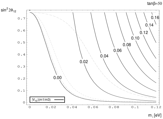
Figure 2: Contour plot of $|V_{13}|(m_{1}/m_{3})$ in $\sin^{2}2\theta_{12}$ and $m_{1}$ plain for $\tan\beta=50$. We use same values as Fig. 1 for experimental values. Gray curves show the $\alpha_{0}$ values as in Fig. 1.

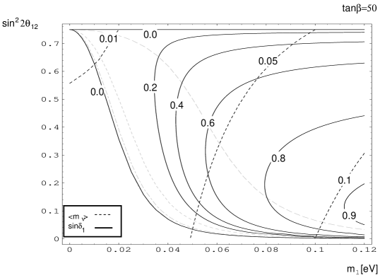
Figure 3: Contour plot of $\sin\delta_{1}$ and $\langle m_{\nu}\rangle$ for $\tan\beta=50$. We use same values as Fig. 1 for experimental values. Solid curves denote $\sin\delta_{1}$ and dashed curves denote $\langle m_{\nu}\rangle$. Gray curves show the $\alpha_{0}$ values as in Fig. 1.

Figure 4: Contour plot of $\alpha_{0}$ in $\sin^{2}2\theta_{12}$ and $m_{1}$ plain to reconstruct the experimental value of $\theta_{\odot}$ in the case of $\tan\beta=20$. We use same values as Fig. 1 for experimental values. The allowed region is between $\alpha_{0}=\pi$ and $\alpha_{0}=0$ lines.

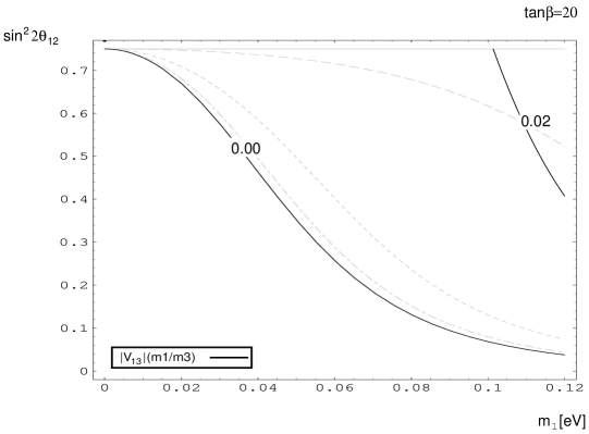
Figure 5: Contour plot of $|V_{13}|(m_{1}/m_{3})$ in $\sin^{2}2\theta_{12}$ and $m_{1}$ plain for $\tan\beta=20$. We use same values as Fig. 1 for experimental values. Gray curves show the $\alpha_{0}$ values as in Fig. 4.

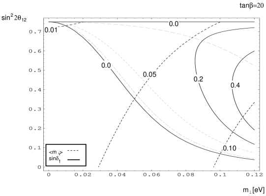
Figure 6: Contour plot of $\sin\delta_{1}$ and $\langle m_{\nu}\rangle$ for $\tan\beta=20$. We use same values as Fig. 1 for experimental values. Solid curves denote $\sin\delta_{1}$ and dashed curves denote $\langle m_{\nu}\rangle$. Gray curves show the $\alpha_{0}$ values as in Fig. 4.

5 Summary and discussions

In this paper, we discuss a class of neutrino mass matrix which predicts zero or a small value of $|V_{13}|$ and found the inequality in Eq. (28). This constraint gives a severe restriction for model building of neutrino mass matrix. In particular, the model which predicts a larger value of $\tan^{2}\theta_{12}$ at $M_{R}$ scale than the experimental value obtained from the solar neutrino mixing is excluded. As a result, the bi-maximal mixing scheme at $M_{R}$ scale is excluded, if the experimental value $\tan^{2}\theta_{\odot}<1$ is established.

In this model, $|V_{13}|$ in Eq. (19) at $m_{Z}$ which is induced radiatively may not be small as it is shown in Fig. 2, if the neutrino mass $m_{1}$ is of order 0.05 eV. The Dirac phase $\delta_{1}$ in Eq. (29) at $m_{Z}$ which is also induced may not be small in general as we see in Fig. 3. The effective neutrino mass $\langle m_{\nu}\rangle$ in Eq. (30) is expected to be of order 0.05 eV. All these values for $|V_{13}|$, $\delta_{1}$ and $\langle m_{\nu}\rangle$ depend crucially on the mass $m_{1}$ which is assumed to be around 0.05 eV.

The fact that Majorana phases at $M_{R}$ scale can induce a Dirac phase pushes our dream further to consider the possible relation between a Dirac phase which appears in the neutrino oscillations and the Majorana phase which appears in the leptogenesis. We believe such scenario does exist and the finding of the missing link will be the most wonderful and fruitful project.

Recently, Antusch et al.AKLR studied the quantum effect for the neutrino mass matrix which reproduces the Bi-Maximal mixing at the GUT scale, $M_{G}$. They considered the quantum effect due to heavy Majorana neutrinos. They considered two cases, (i) the standard model (SM) and (ii) the MSSM with $\tan\beta=5$. In both cases, the quantum effect from the lightest heavy Majorana neutrino mass, $M_{R}$ to $m_{Z}$ is very small so that it can be neglected. Therefore, they considered a possibility that that $\tan^{2}\theta_{\rm sol}=1$ at $M_{G}$ reduces to the experimental value $\tan^{2}\theta_{\rm sol}=0.34$ at $M_{R}$ by the radiative correction. They found it possible in a special situation where the Dirac mass matrix is in the form of $m_{D}=(v/\sqrt{2}){\rm diag}(1,\epsilon^{\prime},\epsilon^{\prime 2})$ with $\epsilon^{\prime}<1$, which in turn means that $M_{R}\sim 10^{14}$GeV. This model has two special features: One is that the Dirac mass matrix has the inverse mass hierarchy which disagrees with the naive expectation from the GUT scenario. The other is that the scale of $M_{R}$ is larger than the ordinary expectation, $M_{R}\sim 10^{13}$GeV in order to have larger Yukawa coupling constants, $y_{\nu}$, related to the Dirac neutrino mass. In our case, we consider the large $\tan\beta$ case so that Yukawa coupling constants $y_{\nu}$ are small. Thus, the correction is negligible and our result is valid even at $M_{G}$.

Acknowledgment This work is supported in part by the Japanese Grant-in-Aid for Scientific Research of Ministry of Education, Science, Sports and Culture, No.12047218.

Appendix A: Diagonalization of the neutrino mass matrix

We define ${\rm diag}(1,1,\alpha)O=OX$,

$$X = 1-\epsilon O^{T}{\rm diag}(0,0,1)O$$ (A.1)

$$= 1-\epsilon\begin{pmatrix}s_{12}^{2}s_{23}^{2}&s_{12}c_{12}s_{23}^{2}&s_{12}s_{23}c_{23}\cr s_{12}c_{12}s_{23}^{2}&c_{12}^{2}s_{23}^{2}&c_{12}s_{23}c_{23}\cr s_{12}s_{23}c_{23}&c_{12}s_{23}c_{23}&c_{23}^{2}\cr\end{pmatrix}\;,$$

where $\epsilon=1-\alpha$ is a small positive quantity and its value is given in Eq. (8), then we consider the mass matrix transformed by $O$ as

$$\bar{m}_{\nu}\equiv O^{T}m_{\nu}(m_{Z})O=XD_{\nu}X^{T}\;.$$ (A.2)

Now, we diagonalize $\bar{m}_{\nu}$.

In order to diagonalize this matrix directly, we consider the Hermite matrix $\bar{m}_{\nu}^{\dagger}\bar{m}_{\nu}$

$$\bar{m}_{\nu}^{\dagger}\bar{m}_{\nu}\simeq(1-4\epsilon s_{12}^{2}s_{23}^{2})M_{1}^{2}+Y\;,$$ (A.3)

where elements of $Y$ are given up to the 1st order of $\epsilon$ as

$$Y_{11} = 0\;,\;Y_{22}=\tilde{\Delta}_{21}\;,\;Y_{33}=\tilde{\Delta}_{31}\;,$$

$$Y_{12} = Y_{21}^{*}=-2\epsilon s_{12}c_{12}s_{23}^{2}(M_{1}^{2}+M_{2}^{2}+2M_{1}M_{2}e^{i\alpha_{0}})M_{1}^{2}\;,$$

$$Y_{13} = Y_{31}^{*}=-\epsilon s_{12}s_{23}c_{23}(M_{1}^{2}+M_{3}^{2}+2M_{1}M_{3}e^{i\beta_{0}})\;,$$

$$Y_{23} = Y_{32}^{*}=-\epsilon c_{12}s_{23}c_{23}(M_{2}^{2}+M_{3}^{2}+2M_{2}M_{3}e^{i(\beta_{0}-\alpha_{0})})\;.$$

$$\tilde{\Delta}_{21} = \Delta_{21}-4\epsilon s_{23}^{2}(c_{12}^{2}M_{1}^{2}-s_{12}^{2}M_{2}^{2})\;,$$

$$\tilde{\Delta}_{31} = \Delta_{31}-4\epsilon(c_{23}^{2}M_{3}^{2}-s_{12}^{2}s_{23}^{2}M_{1}^{2})\;.$$ (A.5)

Since $\bar{m}_{\nu}^{\dagger}\bar{m}_{\nu}$ is an Hermite matrix, it is diagonalized by the unitary transformation as $V^{\dagger}\bar{m}_{\nu}^{\dagger}\bar{m}_{\nu}V\simeq(1-4\epsilon s_{12}^{2}s_{23}^{2})M_{1}^{2}+V^{\dagger}YV$. The diagonalization of the matrix $Y$ can be achieved by using the see-saw technique, because $|Y_{33}|$ is much larger than all other terms. That is, by using the unitary matrix

$$V_{3}\simeq\begin{pmatrix}1&0&\frac{Y_{13}}{Y_{33}}\cr 0&1&\frac{Y_{23}}{Y_{33}}\cr-\frac{Y_{13}^{*}}{Y_{33}}&-\frac{Y_{23}^{*}}{Y_{33}}&1\cr\end{pmatrix}\;.$$ (A.6)

$Y$ is block diagonalized in a good accuracy as

$$V_{3}^{\dagger}YV_{3} \simeq \begin{pmatrix}-\frac{2|Y_{13}|^{2}}{Y_{33}}&Y_{12}-\frac{2Y_{13}Y_{23}^{*}}{Y_{33}}&0\cr Y_{12}^{*}-\frac{2Y_{13}^{*}Y_{23}}{Y_{33}}&Y_{22}-\frac{2|Y_{23}|^{2}}{Y_{33}}&0\cr 0&0&Y_{33}+\frac{|Y_{13}|^{2}+|Y_{23}|^{2}}{Y_{33}}\cr\end{pmatrix}$$ (A.7)

$$\simeq \begin{pmatrix}0&Y_{12}&0\cr Y_{12}^{*}&Y_{22}&0\cr 0&0&Y_{33}\cr\end{pmatrix}\;,$$

where in the last equation, we neglected the see-saw induced terms because $|Y_{13}/Y_{33}|$ and $|Y_{23}/Y_{33}|$ are much smaller than 1 and $Y_{13}$ and $Y_{23}$ are same order of $Y_{12}$ and $Y_{22}$.

In the following, we use $M_{1}=M_{2}$ for terms proportional to $\epsilon$ to simplify the expression. The matrix in Eq. (A7) is diagonalized by

$$V_{12}=\begin{pmatrix}c&-se^{i\alpha_{0}/2}&0\cr se^{-i\alpha_{0}/2}&c&0\cr 0&0&1\cr\end{pmatrix}\;,$$ (A.8)

with $c=\cos\theta$ and $s=\sin\theta$ as

$$V_{12}^{\dagger}(V_{3}^{\dagger}YV_{3})V_{12}={\rm diag}(\lambda_{1},\lambda_{2},\lambda_{3})\;,$$ (A.9)

where

$$\tan 2\theta=\frac{4\epsilon M_{1}^{2}\sin 2\theta_{12}s_{23}^{2}\cos\frac{\alpha_{0}}{2}}{\tilde{\Delta}_{21}}\;,$$ (A.10)

and

$$\lambda_{1}\simeq\frac{\tilde{\Delta}_{21}}{2}\left(1-\frac{1}{\cos 2\theta}\right)\;,\;\;\lambda_{2}\simeq\frac{\tilde{\Delta}_{21}}{2}\left(1+\frac{1}{\cos 2\theta}\right)\;,\;\;\lambda_{3}\simeq\tilde{\Delta}_{31}\;.$$ (A.11)

Neutrino masses at $m_{Z}$ are obtained by $m_{i}^{2}=(1-4\epsilon s_{12}^{2}s_{23}^{2})M_{1}^{2}+\lambda_{i}$ and

$$\Delta m_{\odot}^{2} \equiv m_{2}^{2}-m_{1}^{2}=\frac{\tilde{\Delta}_{21}}{\cos 2\theta}\;,$$

$$\Delta m_{\rm atm}^{2} \equiv m_{3}^{2}-m_{2}^{2}\simeq m_{3}^{2}-m_{1}^{2}\simeq\tilde{\Delta}_{31}\;.$$ (A.12)

We find that the angle $\theta$ is expressed by

$$\sin 2\theta=\frac{4\epsilon M_{1}^{2}\sin 2\theta_{12}s_{23}^{2}\cos\frac{\alpha_{0}}{2}}{\Delta m_{\odot}^{2}}\;.$$ (A.13)

By taking into account of

$$(OV_{3}V_{12})^{T}m_{\nu}(m_{Z})OV_{3}V_{12}\simeq{\rm diag}(m_{1},m_{2}e^{i\alpha_{0}},m_{3}e^{i\beta_{0}})\;,$$ (A.14)

with $m_{i}>0$, we find the mixing matrix $V$ which satisfies $V^{T}m_{\nu}(m_{Z})V={\rm diag}(m_{1},m_{2},m_{3})$ is $V\equiv OV_{3}V_{12}{\rm diag}(1,e^{-i\alpha_{0}/2},e^{-i\beta_{0}/2})$ is given by

$$V\simeq\begin{pmatrix}c_{12}c-s_{12}se^{-i\alpha_{0}/2}&-(s_{12}c+c_{12}se^{i\alpha_{0}/2})&-|V_{13}|e^{i\rho}\cr c_{23}(s_{12}c+c_{12}se^{-i\alpha_{0}/2})&c_{23}(c_{12}c-s_{12}se^{i\alpha_{0}/2})&-s_{23}\cr s_{23}(s_{12}c+c_{12}se^{-i\alpha_{0}/2})&s_{23}(c_{12}c-s_{12}se^{i\alpha_{0}/2})&c_{23}\cr\end{pmatrix}\begin{pmatrix}1&0&0\cr 0&e^{-i\alpha_{0}/2}&0\cr 0&0&e^{-i\beta_{0}/2}\cr\end{pmatrix}\;,$$

where

$$|V_{13}| = \frac{\epsilon m_{1}m_{3}\sin 2\theta_{12}\sin 2\theta_{23}\sin\frac{\alpha_{0}}{2}}{\tilde{\Delta}m^{2}_{31}}\;,$$

$$\rho = \frac{\pi}{2}-\frac{\alpha_{0}}{2}+\beta_{0}\;.$$ (A.16)

References

(1)
Y. Fukuda et al. [Super-Kamiokande Collaboration],
Phys. Rev. Lett. 81, 1562 (1998).
(2)
Q. R. Ahmad et al. [SNO Collaboration],
Phys. Rev. Lett. 87, 071301 (2001);
Q. R. Ahmad et al. [SNO Collaboration],
arXiv:nucl-ex/0204009.
(3)
S. Fukuda et al. [SuperKamiokande Collaboration],
Phys. Rev. Lett. 86, 5651 (2001).
(4)
A. de Gouvea, A. Friedland and H. Murayama,
Phys. Lett. B 490, 125 (2000).
(5)
C. Bemporad [Chooz Collaboration],
Nucl. Phys. Proc. Suppl. 77, 159 (1999);
M. Apollonio et al. [CHOOZ Collaboration],
Phys. Lett. B 466, 415 (1999).
(6)
Z. Maki, M. Nakagawa and S. Sakata,
Prog. Theor. Phys. 28, 870 (1962).
(7)
S. M. Bilenky, J. Hosek and S. T. Petcov,
Phys. Lett. B 94, 495 (1980).
(8)
M. Doi, T. Kotani, H. Nishiura, K. Okuda and E. Takasugi,
Phys. Lett. B 102, 323 (1981).
(9)
J. Schechter and J. W. Valle,
Phys. Rev. D 22, 2227 (1980);
Phys. Rev. D 23, 1666 (1981).
(10)
F. Vissani,
arXiv:hep-ph/9708483;
V. D. Barger, S. Pakvasa, T. J. Weiler and K. Whisnant,
Phys. Lett. B 437, 107 (1998);
A. J. Baltz, A. S. Goldhaber and M. Goldhaber,
Phys. Rev. Lett. 81, 5730 (1998).
(11)
H. Harari, H. Haut and J. Weyers,
Phys. Lett. B 78, 459 (1978);
Y. Koide,
Phys. Rev. D 39, 1391 (1989);
H. Fritzsch and Z. Z. Xing,
Phys. Lett. B 372, 265 (1996);
M. Fukugita, M. Tanimoto and T. Yanagida,
Phys. Rev. D 57, 4429 (1998).
(12)
N. Cabibbo,
Phys. Lett. B 72, 333 (1978);
L. Wolfenstein,
Phys. Rev. D 18, 958 (1978);
V. D. Barger, K. Whisnant and R. J. Phillips,
Phys. Rev. D 24, 538 (1981);
A. Acker, J. G. Learned, S. Pakvasa and T. J. Weiler,
Phys. Lett. B 298, 149 (1993);
R. N. Mohapatra and S. Nussinov,
Phys. Lett. B 346, 75 (1995);
P. F. Harrison, D. H. Perkins and W. G. Scott,
Phys. Lett. B 349, 137 (1995);
Phys. Lett. B 374, 111 (1996);
Phys. Lett. B 396, 186 (1997);
Phys. Lett. B 458, 79 (1999);
C. Giunti, C. W. Kim and J. D. Kim,
Phys. Lett. B 352, 357 (1995);
R. Foot, R. R. Volkas and O. Yasuda,
Phys. Lett. B 433, 82 (1998).
(13)
K. Fukuura, T. Miura, E. Takasugi and M. Yoshimura,
Phys. Rev. D 61, 073002 (2000).
(14)
K.S. Babu, C.N. Leung and J.Pantaleone,
Phys. Lett. B 319, 191 (1993);
N. Haba and N. Okamura,
Eur. Phys. J. C 14, 347 (2000);
T. Miura, E. Takasugi and M. Yoshimura,
Prog. Theor. Phys. 104, 1173 (2000).
(15)
J. A. Casas, J. R. Espinosa, A. Ibarra and I. Navarro,
JHEP 9909, 015 (1999);
Nucl. Phys. B 573, 652 (2000);
K. R. Balaji, A. S. Dighe, R. N. Mohapatra and M. K. Parida,
Phys. Rev. Lett. 84, 5034 (2000);
N. Haba, Y. Matsui, N. Okamura and T. Suzuki,
Phys. Lett. B 489, 184 (2000).
(16)
N. Haba, Y. Matsui and N. Okamura,
Eur. Phys. J. C 17, 513 (2000);
N. Haba, Y. Matsui, N. Okamura and M. Sugiura,
Prog. Theor. Phys. 103, 145 (2000).
(17)
S. Antusch, j. Kersten, M. Lindner and M. Ratz,
arXiv:hep-ph/0203233;
S. Antusch, j. Kersten, M. Lindner and M. Ratz,
arXiv:hep-ph/0206078.