Isolating a light Higgs boson
from the di-photon background at the LHC

Abstract

We compute the QCD corrections to the gluon fusion subprocess $gg\rightarrow\gamma\gamma$, which forms an important component of the background to the search for a light Higgs boson at the LHC. We study the dependence of the improved $pp\rightarrow\gamma\gamma X$ background calculation on the factorization and renormalization scales, on various choices for photon isolation cuts, and on the rapidities of the photons. We also investigate ways to enhance the statistical significance of the Higgs signal in the $\gamma\gamma$ channel.

I Introduction

The nature of electroweak symmetry breaking remains a mystery, despite decades of theoretical and experimental study. In the Standard Model, the masses for the $W$ and $Z$ bosons, quarks and charged leptons are all generated by the Higgs mechanism. This mechanism leaves as its residue the Higgs boson, the one undetected elementary particle of the Standard Model, and the only scalar Higgs . Its properties are completely specified once its mass is determined. Alternatives to, or extensions of, the Standard Model electroweak symmetry breaking mechanism typically also include one or more Higgs particles. Experiments over the next decade at the Fermilab Tevatron and the CERN Large Hadron Collider (LHC) should shed considerable light on electroweak symmetry breaking, in particular by searching for these Higgs bosons, and measuring their masses, production cross sections, and branching ratios.

There are good reasons to believe that at least one Higgs particle will be fairly light. The Standard Model Higgs boson mass is bounded from above by precision electroweak measurements, $m_{H}\buildrel<\over{{}_{\sim}}196$–$230$ GeV at 95% CL HiggsRadCorr . In the Minimal Supersymmetric Standard Model (MSSM), the lightest Higgs boson is predicted to have a mass below about 135 GeV SusyHiggs ; over much of the parameter space it has properties reasonably similar to the Standard Model Higgs boson. There are also hints of a signal in the direct search in $e^{+}e^{-}\rightarrow HZ$ at LEP2, just beyond the lower mass limit of 114.1 GeV LEP2Limit . The corresponding lower limit on the lightest scalar in the MSSM is only 91.0 GeV LEP2MSSMLimit , because the $HZZ$ coupling can be suppressed in some regions of parameter space.

Run II of the Tevatron can exclude Standard Model Higgs masses up to $\approx 180$ GeV with 15 fb^-1 per experiment. However, at this integrated luminosity a 5$\sigma$ discovery will be difficult to obtain RunIIExpectations for a mass much beyond the LEP2 limit. Also, the Higgs decay modes relevant for searches at the Tevatron, $H\rightarrow b\bar{b}$ and $W^{+}W^{-}$, do not lend themselves to a precise measurement of the Higgs mass. The LHC will completely cover the low mass region preferred by precision electroweak fits and the MSSM, as well as much higher masses. For $m_{H}<140$ GeV, the most important mode involves production via gluon fusion, $gg\rightarrow H$, followed by the rare decay into two photons, $H\rightarrow\gamma\gamma$ HggVertex ; Higgsgammagamma . Although this mode has a very large continuum $\gamma\gamma$ background HBkgdgammagamma , the narrow width of the Higgs boson, combined with the mass resolution of order 1% achievable in the LHC detectors, allows one to measure the background experimentally and subtract it from a putative signal peak ATLAS ; CMS ; Tisserand ; Wielers .

For the same mass range of $m_{H}<140$ GeV at the LHC, Higgs production via weak boson fusion, $qq^{\prime}\rightarrow qq^{\prime}W^{+}W^{-}\rightarrow qq^{\prime}H$, followed by (virtual) weak boson decay, $H\rightarrow W^{+}W^{-}\rightarrow e^{\pm}\mu^{\mp}/{\hbox{\kern-6.0pt$p_{\rm T}$}}$, is also promising, even for Higgs masses as low as the LEP2 limit RZ . On the other hand, a mass determination from this mode, or from weak boson fusion followed by $H\rightarrow\tau^{+}\tau^{-}$ RZH , cannot compete with the $\gamma\gamma$ mode, although these modes certainly offer very useful branching ratio information.

The purpose of this paper is to provide an improved calculation of the prompt (i.e. not from hadron decay) di-photon background to Higgs production at the LHC, in particular by computing QCD corrections to the gluon fusion subprocess. Although the background will be measured at the LHC, it is still useful to have a robust theoretical prediction in order to help validate the quantitative understanding of detector performance. Perhaps more importantly, the theoretical prediction can be used to systematically study the dependence of the signal relative to the background on various kinematic cuts, providing information which can be used to optimize Higgs search strategies. As a side benefit, one can improve the predictions for a variety of di-photon distributions that can be measured.

The process $pp\rightarrow\gamma\gamma X$ proceeds at lowest order via the quark annihilation subprocess $q{\bar{q}}\rightarrow\gamma\gamma$, which is independent of the strong coupling $\alpha_{s}$. The next-to-leading-order (NLO) corrections to this subprocess have been incorporated into a number of Monte Carlo programs TwoPhotonBkgd1 ; DIPHOX . However, the gluon distribution in the proton becomes very large at small $x$, making formally higher order corrections involving gluon initial states very significant for the production of low-mass systems at the LHC. Gluons can fuse to photon pairs through one-loop quark box diagrams such as the one shown in fig. 1(a). The order $\alpha_{s}^{2}$ contribution to $pp\rightarrow\gamma\gamma X$ from $gg\rightarrow\gamma\gamma$ is indeed comparable to the leading-order quark annihilation contribution HBkgdgammagamma ; ADW ; TwoPhotonBkgd1 ; DIPHOX . (In fact, the NLO correction to quark annihilation, including the $qg\rightarrow\gamma\gamma q$ amplitude, can also be as large as either of these terms.) Hence, to reduce the uncertainty on the total $\gamma\gamma$ production rate, we have computed the contributions of the $gg\rightarrow\gamma\gamma$ subprocess at its next-to-leading-order, which we shall call “NLO”, even though it is formally N³LO as far as the whole process $pp\rightarrow\gamma\gamma X$ is concerned.

The NLO gluon fusion computation has two matrix-element ingredients:

• The virtual corrections to $gg\rightarrow\gamma\gamma$, involving two-loop diagrams such as the one in fig. 1(b), which were computed recently GGGamGam using the integration methods developed in refs. TwoloopIntegrals .

• The effects of gluon bremsstrahlung, through the one-loop amplitude for $gg\rightarrow\gamma\gamma g$, including pentagon diagrams as depicted in fig. 1(c). The $gg\rightarrow\gamma\gamma g$ amplitude can be obtained from the one-loop five-gluon matrix elements FiveGluon by summing over permutations of the external legs GGGamGamGa ; GGGamGamGb .

Both the virtual and real corrections have been evaluated in the limit of vanishing quark masses. In the range of di-photon invariant masses relevant for the Standard Model and MSSM Higgs searches, 90–150 GeV, this is an excellent approximation. The masses of the five light quarks are all much less than the scale of the process. The top quark contribution is negligible until the invariant mass approaches $2m_{t}\approx 350$ GeV; at 150 GeV, it is still well under one percent of the total quark loop contribution. The virtual and real corrections are separately infrared divergent. We have used the dipole formalism CataniSeymour to combine them into a finite result, in a numerical program that can compute general kinematic distributions.

Figure 1: Sample quark loop diagrams contributing to $pp\rightarrow\gamma\gamma X$, which are computed in this paper: (a) the leading order gluon fusion subprocess $gg\rightarrow\gamma\gamma$, (b) the virtual correction to this subprocess, and (c) the radiative process $gg\rightarrow\gamma\gamma g$.

Prompt photons are not only produced directly in hard processes, but also via fragmentation from quarks and gluons. As discussed in ref. DIPHOX , even though the separation into direct and fragmentation contributions is somewhat arbitrary, it is still very useful to track the pieces separately. The fragmentation processes occur at low $p_{\rm T}$ with respect to a neighboring jet. They can only be computed with the aid of nonperturbative information, in the form of the quark and gluon fragmentation functions to a photon, $D_{\gamma/(q\ {\rm or}\ g)}(z,\mu_{F})$. Here $z$ is the fractional collinear momentum carried by the photon, measured relative to the momentum of the parton which fragments into it, and $\mu_{F}$ is the factorization scale used to separate the hard and soft processes. The inclusive di-photon production rate at the LHC is actually dominated by the single fragmentation process, e.g. the partonic subprocess $qg\rightarrow\gamma q$, followed by the fragmentation $q\rightarrow\gamma X$. Even the double fragmentation process, e.g. $gg\rightarrow q{\bar{q}}$ followed by the fragmentations $q\rightarrow\gamma X$ and ${\bar{q}}\rightarrow\gamma X$, can exceed the direct contribution in the 80–140 GeV range for $M_{\gamma\gamma}$ DIPHOX .

However, fragmentation contributions can be efficiently suppressed by photon isolation cuts DIPHOX . Such cuts are mandatory in order to suppress the very large reducible experimental background where photons are faked by jets, or more generally by hadrons. In particular, $\pi^{0}$s at large $p_{\rm T}$ decay into two nearly collinear photons, which can be difficult to distinguish from a single photon. The standard method for defining an isolated photon is to first draw a circle of radius $R$ in the plane of pseudorapidity, $\eta=\ln\tan(\theta/2)$, and azimuthal angle, $\phi$, centered on the photon candidate. The amount of transverse hadronic energy in this circle, or cone, is required to be less than some specified amount, $E_{\rm T\,max}$. Here, $R$ and $E_{\rm T\,max}$ may in principle be varied independently. Although photon isolation is improved by increasing $R$ and decreasing $E_{\rm T\,max}$, this cannot be done indefinitely, for both theoretical and experimental reasons. Theoretically, it is not infrared-safe to forbid all gluon radiation in a finite patch of phase space, so any prediction would have large uncontrolled corrections. Experimentally, fluctuations in the number of soft hadrons from the hard scattering, the underlying event, and other minimum bias events in the same bunch crossing, plus detector noise, impose a lower limit on the $E_{\rm T\,max}$ that can be required for isolation, at a given $R$.

A typical choice of isolation criteria in past LHC studies has been $R=0.4$ and $E_{\rm T\,max}=5$ or 15 GeV DIPHOX . The experimental optimization of these variables has often been made with the suppression of the huge reducible background from jet fakes as a primary criterion ATLAS ; CMS ; Tisserand ; Wielers . This criterion is very understandable in the light of how poorly this background is understood; it depends on the tails of distributions, such as the very hard ($z\approx 1$) tail of parton fragmentation to $\pi^{0}$s PiBkgd . Nevertheless, it is estimated that this background can be reduced to the order of 10–20% of the irreducible $\gamma\gamma$ background, so that one should try to optimize with respect to the latter background as well. We shall investigate the behavior of the irreducible $\gamma\gamma$ background, as well as the Higgs signal, as the cone size $R$ is increased, while also increasing the transverse energy allowed into the cone.

An alternative “smooth” cone isolation criterion has been proposed by Frixione Frixione , in which a continuous set of cones with $r<R$ are defined, and the transverse energy permitted inside $r$, $E_{\rm T}(r)$, decreases to zero as $r$ does. This criterion has the theoretical advantage that it entirely suppresses the more poorly known fragmentation contribution, while still being infrared safe. Experimentally, however, this theoretical ideal may be difficult to achieve with a detector of finite granularity, and taking into account the transverse extent of the photon’s electromagnetic shower Wielers . Nevertheless, we shall study the behavior of Higgs signal and background for a few versions of the smooth cone criterion as well.

The fragmentation contributions are technically involved to compute at NLO. Their implementation requires, for example, all the one-loop four-parton matrix elements and tree-level five-parton matrix elements, as well as convolution with fragmentation functions. Fortunately, a flexible program is available, DIPHOX DIPHOX ; PiBkgd , which incorporates at NLO the quark annihilation direct subprocess, plus single and double fragmentation. It also contains the gluon fusion subprocess at leading order. We have used DIPHOX to produce all the non-gluon fusion contributions to $pp\rightarrow\gamma\gamma X$ for the case of standard cone isolation. These were then combined with the results of our NLO implementation of gluon fusion. (We have also checked the DIPHOX implementation of the leading order gluon fusion contribution against ours, and they agree perfectly.) For the case of smooth cone isolation, where fragmentation contributions are absent, we have implemented the $q{\bar{q}}\rightarrow\gamma\gamma$ direct subprocess at NLO ourselves, as well as the gluon fusion subprocess.

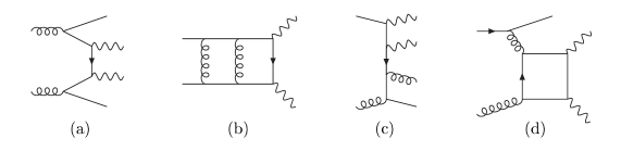
Figure 2: Sample diagrams for contributions to $pp\rightarrow\gamma\gamma X$ which are not treated in this paper, although they are of order $\alpha_{s}^{2}$: (a) the tree-level subprocess $gg\rightarrow\gamma\gamma q{\bar{q}}$, (b) doubly virtual correction to $q{\bar{q}}\rightarrow\gamma\gamma$, (c) doubly real correction to $q{\bar{q}}\rightarrow\gamma\gamma$, of the form $qg\rightarrow\gamma\gamma gq$, and (d) the process $qg\rightarrow\gamma\gamma q$ via a quark box.

Since we are computing only a selection of the contributions to $pp\rightarrow\gamma\gamma X$ at order $\alpha_{s}^{2}$ and $\alpha_{s}^{3}$, we should make a few remarks about contributions we have omitted, at least those appearing at order $\alpha_{s}^{2}$. Figure 2 indicates a few such contributions. Perhaps most worrisome at first glance is the tree-level cross section for $gg\rightarrow\gamma\gamma q{\bar{q}}$, as shown in fig. 2(a). This subprocess can utilize the large gluon-gluon luminosity, is only of order $\alpha_{s}^{2}$, and has not yet been computed to our knowledge. In addition, it can be enhanced by $\gamma q$ collinear singularities if the isolation cut is not too severe. It has a double collinear singularity related to the $g\rightarrow q{\bar{q}}$ splitting process, so that this contribution should depend on the factorization scale through terms proportional to $\alpha_{s}^{2}(\ln{\mu_{F}})^{n}$ with $n=1,2$. Although this contribution alone does not cancel the full dependence on $\mu_{F}$ to order $\alpha_{s}^{2}$, it does cancel the terms in $d\sigma/d(\ln\mu_{F})$ that are enhanced by two factors of the gluon density and are potentially the largest. Therefore, it is reasonable to consider the $gg\rightarrow\gamma\gamma X$ contributions as a first approximation to the full NNLO calculation. A study of the similar subprocesses, $gg\rightarrow WVq{\bar{q}}^{\prime}$ where $V=\gamma$ or $Z$, was recently carried out, with the conclusion that their effects are actually quite small, 5% or less (and negative), with respect to the lower-order contributions of the $q{\bar{q}}$ and $qg$ initial states AdFS . Assuming that these results also hold for the $\gamma\gamma$ final state, our neglect of $gg\rightarrow\gamma\gamma q{\bar{q}}$ should be tolerable.

Other order $\alpha_{s}^{2}$ corrections to the quark annihilation subprocess include the two-loop virtual corrections shown in fig. 2(b), which also have been computed recently QQGamGam , and real corrections, such as from $qg\rightarrow\gamma\gamma gq$ in fig. 2(c). The numerical implementation of these corrections involve doubly unresolved parton configurations and remain to be performed. Because the $qg\rightarrow\gamma\gamma q$ amplitude provides such a large NLO correction to the quark annihilation subprocess, the order $\alpha_{s}^{2}$ contributions arising from the $qg$ initial state could be reasonably important. The $qg$ initial-state contributions may be more tractable than the full order $\alpha_{s}^{2}$ corrections to the quark annihilation subprocess, because of fewer soft gluon singularities.

There are actually three other ways for the quark box responsible for $gg\rightarrow\gamma\gamma$ to contribute to the $pp\rightarrow\gamma\gamma X$ cross section at order $\alpha_{s}^{2}$. The quark box can be incorporated into the one-loop $qg\rightarrow\gamma\gamma q$ amplitude shown in fig. 2(d), which can then interfere with the tree-level $qg\rightarrow\gamma\gamma q$ amplitude. However, such a contribution only gets to utilize one gluon distribution function at small $x$, not two. It is likely to be smaller than the other order $\alpha_{s}^{2}$ $qg$ initial-state contributions just mentioned, given that it lacks both initial- and final-state singularities. (The loop and tree amplitudes each have square-root collinear singularities, but they appear in different collinear limits, so that the phase space integral of the amplitude product remains finite.) The quark box contribution to the crossed process $q{\bar{q}}\rightarrow\gamma\gamma g$ is also infrared finite, and lacks any small $x$ gluon enhancement, so it should be even smaller than the $qg\rightarrow\gamma\gamma q$ case. Finally, there is a two-loop virtual correction to $q{\bar{q}}\rightarrow\gamma\gamma$ containing the quark box (not shown here), which can interfere with the tree amplitude at order $\alpha_{s}^{2}$. This particular correction is also infrared finite, and does not benefit from any small $x$ gluon distribution. Numerical evaluation of the expression in ref. QQGamGam shows that its magnitude never exceeds 0.3% of the Born quark annihilation cross section (its sign is negative for all relevant, central scattering angles), so we are justified in neglecting it.

In this paper we also investigate the effects of isolation cuts and other kinematic features of the Higgs signal vs. the QCD background. Intuitively, one might expect the irreducible background to diminish more rapidly than the signal as one imposes more severe photon isolation requirements for the following reason: The largest component of the irreducible background, for typical isolation cuts, comes from the subprocess $qg\rightarrow\gamma\gamma q$, even after we include the NLO corrections to gluon fusion. The $qg$-initiated subprocess has final-state singularities when the quark is collinear with either of the photons, which of course require some kind of photon isolation to make finite. Thus, the contribution of this subprocess can be significantly reduced with tighter isolation cuts. On the other hand, the dominant Higgs production process, $gg\rightarrow HX$, even at higher orders where additional partons are radiated, clearly does not give rise to partons that are preferentially near the photons.

There are at least two different ways to make the photon isolation more severe. One way is to strengthen the isolation cone, for example by increasing its radius $R$. A second approach is to impose a jet veto Tisserand in the neighborhood of the photon candidate, on top of a “standard” isolation requirement. For example, one may forbid events having a jet with $E_{\rm T}>E_{\rm T\,jet}$ whose axis is within a distance $R_{\rm jet}$ in $(\eta,\phi)$ space from either photon candidate, where $R_{\rm jet}>R$. The two approaches are depicted in fig. 3. The small inner cone corresponds to a standard photon isolation cone, e.g. with radius $R=0.4$. The outer cone could correspond to a larger isolation cone, e.g. with radius $R=1$ or $R=2$. Alternatively, it could represent the radius $R_{\rm jet}$ within which jets, such as the one depicted, are vetoed against.

At the level of a NLO parton calculation, the jet veto approach is not too different from the large cone approach, if one chooses $R_{\rm jet}$ and $E_{\rm T\,jet}$ to be equal to the large cone values of $R$ and $E_{\rm T\,max}$, respectively. The reason is that for the direct contributions the hadronic energy is deposited as a single parton. However, the jet veto approach is probably preferable for experimental reasons. The hadronic energy represented by the final state quark in the background process $qg\rightarrow\gamma\gamma q$ should typically be deposited in the form of a jet. In contrast, an equivalent amount of energy originating from either soft hadrons from overlapping events, or detector noise, will usually be uniformly distributed in $(\eta,\phi)$, and so will be less likely to form a jet. Thus when a signal event is accompanied by such energy, it is less likely to be discarded in the case of a jet veto, compared with the case of a standard or smooth isolation cone of large size.

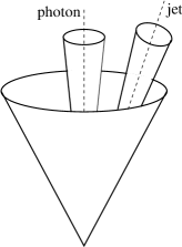
Figure 3: Illustration of two possible ways to strengthen photon isolation, beyond the “standard” isolation represented by the inner cone. One can either increase the cone radius to the large outer one shown, or one can veto on jets within such a radius.

Another feature distinguishing the two photons from Higgs decay from those produced directly is their angular distribution. The $q{\bar{q}}$- and $qg$-initiated components of the background have $t$-channel fermion exchanges that tend to yield photons toward smaller scattering angles in the $\gamma\gamma$ center-of-mass (for a fixed $M_{\gamma\gamma}$), compared with the decay of the Higgs boson, which is isotropic in $\cos\theta^{*}$. Hence, we will study signal and background distributions in $y^{*}\equiv(y(\gamma_{1})-y(\gamma_{2}))/2$, where the $y(\gamma_{i})$ are the rapidities of the photons. This variable serves as a proxy for $\cos\theta^{*}$, because $\cos\theta^{*}=\tanh y^{*}$ at lowest order.

The remaining variable which describes the Higgs boson kinematics at LO is the rapidity of the Higgs boson itself. This leads us to consider the signal and background distributions of $y_{\gamma\gamma}$, the rapidity of the total di-photon system. To a large extent this distribution is determined by the parton luminosities which are involved in the production process. Since Higgs production is dominated by gluon-gluon fusion, whereas the direct $\gamma\gamma$ background gets comparable contributions from all three initial states, $q\bar{q}$, $qg$, and $gg$, there may be a useful difference in the $y_{\gamma\gamma}$ distribution.

To carry out these studies of the signal as well, we have implemented the gluon fusion production of the Standard Model Higgs boson at NLO, followed by decay to $\gamma\gamma$. We work in the heavy top quark limit, for which an effective $Hgg$ vertex HggVertex suffices to describe the production process at the low Higgs transverse momenta we consider. (We do, however, include the exact $m_{H}/m_{t}$ dependence of the LO term. This has been shown NLOHKfactor to be an excellent approximation to the exact NLO cross section NLOHiggs for the Higgs masses with which we are concerned.) The total Higgs production cross section has recently become available in this limit at NNLO HKNNLO . The corrections from NLO to NNLO are modest. Here we wish to study distributions with kinematical cuts, which have not yet been computed at NNLO. For cuts that select events with nonzero transverse momentum of the Higgs boson (which we do not explicitly consider in this paper), our calculation is only a LO computation; distributions for such quantities at NLO are available elsewhere dFGKRSVN . For the branching ratio ${\rm Br}(H\rightarrow\gamma\gamma)$ we use the program HDECAY HDECAY .

This paper is organized as follows. In section II we outline the NLO gluon fusion computation. In section III we show the effects of the NLO corrections to $gg\rightarrow\gamma\gamma$ on the total $pp\rightarrow\gamma\gamma X$ cross section, using kinematic cuts appropriate to the Higgs search, and concentrating on the comparison with LO and on the scale dependence. In section IV we study the effects of varying the photon isolation criteria, either by increasing the size of the isolation cone, or by imposing a veto on nearby jets. We also compute the distributions in $y^{*}$ and $y_{\gamma\gamma}$, and investigate how they may be used to help distinguish the Higgs signal from the background. In section V we present our conclusions, and the outlook for further improvement of our understanding of the $\gamma\gamma$ background.

II Outline of the Computation

The gluon fusion subprocess begins at one loop. The next-to-leading order corrections to it include two-loop four-point amplitudes and one-loop five-point amplitudes. The calculation of these matrix elements requires a fair amount of work GGGamGam ; FiveGluon ; GGGamGamGa ; GGGamGamGb . However, once the amplitudes are available, the rest of the NLO gluon fusion computation is in all essential respects identical to a conventional NLO computation involving tree-level and one-loop amplitudes. For example, the two-loop amplitudes for $gg\rightarrow\gamma\gamma$ have virtual infrared divergences with the same structure as those of a typical one-loop amplitude. Similarly, the vanishing of the $gg\rightarrow\gamma\gamma$ tree amplitude causes the singular behavior of the $gg\rightarrow\gamma\gamma g$ one-loop amplitude, as the outgoing gluon becomes soft or collinear with an incoming gluon, to have the same form as that of a typical tree amplitude with one additional radiated gluon.

The one-loop gluon fusion helicity amplitudes for the process

$$g(-p_{1},-\lambda_{1})+g(-p_{2},-\lambda_{2})\rightarrow\gamma(p_{3},\lambda_{3})+\gamma(p_{4},\lambda_{4}),$$ (1)

in an “all-outgoing” labelling convention for the momenta $p_{i}$ and helicities $\lambda_{i}$, are given by

$${\cal M}_{gg\rightarrow\gamma\gamma}^{1-{\rm loop}}=4\alpha\alpha_{s}(\mu_{R})\,\delta^{a_{1}a_{2}}\biggl{(}\sum_{j=1}^{N_{\!f}}Q_{j}^{2}\biggr{)}M^{(1)}_{\lambda_{1}\lambda_{2}\lambda_{3}\lambda_{4}}\,,$$ (2)

where $\alpha$ is the QED coupling at zero momentum transfer, $\alpha=1/137.036\ldots$ and $\alpha_{s}(\mu_{R})$ is the running QCD coupling in $\rm\overline{MS}$ scheme, evaluated at renormalization scale $\mu_{R}$. Also, in this formula, $a_{1,2}$ are the adjoint gluon color indices, $Q_{j}$ are the quark charges in units of $e$, the appropriate number of light flavors is ${N_{\!f}}=5$, and we have suppressed overall phases in the amplitudes. The quantities $M^{(1)}_{\lambda_{1}\lambda_{2}\lambda_{3}\lambda_{4}}$ are GGGamGam

$$M_{++++}^{(1)} = 1\,,$$

$$M_{-+++}^{(1)} = M_{+-++}^{(1)}=M_{++-+}^{(1)}=M_{+++-}^{(1)}=1\,,$$

$$M_{--++}^{(1)} = -{1\over 2}{t^{2}+u^{2}\over s^{2}}\Bigl{[}\ln^{2}\Bigl{(}{t\over u}\Bigr{)}+\pi^{2}\Bigr{]}$$

$$\hskip 2.0pt-{t-u\over s}\ln\Bigl{(}{t\over u}\Bigr{)}-1\,,$$

$$M_{-+-+}^{(1)} = -{1\over 2}{t^{2}+s^{2}\over u^{2}}\ln^{2}\Bigl{(}-{t\over s}\Bigr{)}$$

$$\hskip 2.0pt-{t-s\over u}\ln\Bigl{(}-{t\over s}\Bigr{)}-1$$

$$\hskip 2.0pt-i\pi\biggl{[}{t^{2}+s^{2}\over u^{2}}\ln\Bigl{(}-{t\over s}\Bigr{)}+{t-s\over u}\biggr{]}\,,$$

$$M_{+--+}^{(1)} = M_{-+-+}^{(1)}\big{|}_{t\leftrightarrow u}\,,$$ (3)

where $s=(p_{1}+p_{2})^{2}$, $t=(p_{2}+p_{3})^{2}$, $u=(p_{1}+p_{3})^{2}$, and the remaining helicity amplitudes are obtained by parity.

The dimensionally-regularized and renormalized two-loop QCD corrections to these amplitudes can be written as GGGamGam

$${\cal M}_{gg\rightarrow\gamma\gamma}^{2-{\rm loop}} = {2\alpha\alpha_{s}^{2}(\mu_{R})\over\pi}\delta^{a_{1}a_{2}}\biggl{(}\sum_{j=1}^{N_{\!f}}Q_{j}^{2}\biggr{)}$$ (4)

$$\hskip-50.0pt\times\biggl{\{}\Bigl{[}I^{(1)}(\epsilon)+b_{0}\Bigl{(}\ln\Bigl{(}{\mu_{R}^{2}\over s}\Bigr{)}+i\pi\Bigr{)}\Bigr{]}M^{(1)}_{\lambda_{1}\lambda_{2}\lambda_{3}\lambda_{4}}$$

$$\hskip-35.0pt+NF^{\rm\scriptscriptstyle L}_{\lambda_{1}\lambda_{2}\lambda_{3}\lambda_{4}}(s,t)-{1\over N}F^{\rm\scriptscriptstyle SL}_{\lambda_{1}\lambda_{2}\lambda_{3}\lambda_{4}}(s,t)\biggr{\}}\,,$$

where the number of dimensions is $D=4-2\epsilon$, and all the poles in $\epsilon$ are contained in

$$I^{(1)}(\epsilon)=-{e^{-\epsilon\psi(1)}\over\Gamma(1-\epsilon)}\Bigl{[}{N\over\epsilon^{2}}+{b_{0}\over\epsilon}\Bigr{]}\Bigl{(}{\mu_{R}^{2}\over-s}\Bigr{)}^{\epsilon}\,,$$ (5)

with

$$b_{0}={11N-2{N_{\!f}}\over 6}\,,$$ (6)

and the number of colors is $N=3$. The finite expressions $F^{\rm\scriptscriptstyle L}_{\lambda_{1}\lambda_{2}\lambda_{3}\lambda_{4}}(s,t)$ and $F^{\rm\scriptscriptstyle SL}_{\lambda_{1}\lambda_{2}\lambda_{3}\lambda_{4}}(s,t)$ are presented in ref. GGGamGam .

The radiative process,

$$g(-p_{1},-\lambda_{1})+g(-p_{2},-\lambda_{2})$$

$$\hskip 20.0pt\rightarrow\gamma(p_{3},\lambda_{3})+\gamma(p_{4},\lambda_{4})+g(p_{5},\lambda_{5}),$$ (7)

begins at order $\alpha_{s}^{3}$. The squared matrix element, averaged over initial helicities and colors, and summed over final ones, and with a 1/2 for identical final-state photons, is given by GGGamGamGa ; GGGamGamGb

$$\overline{|{\cal M}|^{2}}_{\rm\hskip-4.0ptrad}\equiv\sum_{\rm hel.,color}^{\rule{14.22636pt}{0.56905pt}}|{\cal M}_{gg\rightarrow\gamma\gamma g}^{1-{\rm loop}}|^{2}$$

$$=\ 4\pi\alpha^{2}\alpha_{s}^{3}(\mu_{R}){N\over N^{2}-1}\biggl{(}\sum_{j=1}^{N_{\!f}}Q_{j}^{2}\biggr{)}^{2}$$

$$\hskip 10.0pt\times\sum_{\rm hel.}\Biggl{|}\sum_{\sigma\in{\rm COP}_{4}^{(125)}}A_{5;1}^{[1/2]}(\sigma_{1},\sigma_{2},\sigma_{3},\sigma_{4},\sigma_{5})\Biggr{|}^{2}\,,$$ (8)

where $\sigma_{i}$ label the helicities and momenta of the gluons and photons, and ${\rm COP}_{4}^{(125)}$ denotes the subset of 12 permutations of (1,2,3,4,5) that leave 5 fixed and preserve the cyclic ordering of (1,2,5), i.e. 1 appears before 2. The partial amplitudes $A_{5;1}^{[1/2]}(\sigma)$ are those for five-gluon scattering via a quark loop given in ref. FiveGluon , but with an overall factor of $(4\pi)^{-2}$ removed.

The permutation sum in eq. (8) cancels out all of the virtual divergences of the partial amplitudes, and most of their singularities as momenta become soft and collinear. The only remaining singularities are when the final gluon momentum $p_{5}$ becomes soft, or becomes collinear with either initial gluon momentum, $p_{1}$ or $p_{2}$. In the region, for example, where $p_{5}$ is collinear with $p_{1}$, with $p_{5}\rightarrow-(1-x)p_{1}$, the squared matrix element has the limiting behavior,

$$\overline{|{\cal M}|^{2}}_{\rm\hskip-4.0ptrad}\ \rightarrow\ \overline{|{\cal M}|^{2}}_{\rm\hskip-4.0ptdipole,1},$$ (9)

where

$$\hskip-30.0pt\overline{|{\cal M}|^{2}}_{\rm\hskip-4.0ptdipole,1}\equiv{-1\over 2xp_{1}\cdot p_{5}}\biggl{\{}P_{gg}(x)\times\sum_{\rm hel.,color}^{\rule{14.22636pt}{0.56905pt}}|{\cal M}_{gg\rightarrow\gamma\gamma}^{1-{\rm loop}}|^{2}$$

$$\hskip-30.0pt-2N{1-x\over x}{\rm Re}\biggl{[}{\left\langle 1\,5\right\rangle\left[5\,2\right]\left\langle 2\,1\right\rangle\over\left[1\,5\right]\left\langle 5\,2\right\rangle\left[2\,1\right]}\sum_{\rm hel.,color}^{\rule{14.22636pt}{0.56905pt}^{\prime}}|{\cal M}_{gg\rightarrow\gamma\gamma}^{1-{\rm loop}}|^{2}\biggr{]}\biggr{\}}\,,$$ (10)

with

$$P_{gg}(x)=2N\biggl{[}{x\over 1-x}+{1-x\over x}+x(1-x)\biggr{]}\,,$$ (11)

and the $gg\rightarrow\gamma\gamma$ process has the kinematics $(-xp_{1})+(-p_{2})\rightarrow p_{3}+p_{4}$. The second term involves the spinor products $\left\langle i\,j\right\rangle$ MPReview entering the five-point partial amplitudes. It accounts for nontrivial phase behavior of the amplitudes as $p_{5}$ rotates azimuthally about the $p_{1}$ direction. The primed sum is defined analogously to the unprimed sum, except that in each complex conjugated helicity amplitude the helicity of the gluon with momentum $(-xp_{1})$ is flipped, so that $M^{(1)}_{\lambda_{1}\lambda_{2}\lambda_{3}\lambda_{4}}M^{(1)\,*}_{(-\lambda_{1})\lambda_{2}\lambda_{3}\lambda_{4}}$ appears, and the spinor product overall phases in the amplitudes should also be included GGGamGam .

Integration over these singular phase space regions can be handled by the dipole formalism CataniSeymour , with just two dipole subtractions, one for each initial gluon. The dipole subtraction for gluon 1 is given by eq. (10), where $x=(p_{1}+p_{2}+p_{5})^{2}/(p_{1}+p_{2})^{2}$, and the four-point matrix-elements are evaluated for boosted kinematics: gluon 1 is assigned momentum $(-xp_{1})$, gluon 2 momentum $-p_{2}$ still, and the photon momenta $p_{j}$, $j=3,4$, are set equal to

$$\tilde{p}_{j}^{\mu}=p_{j}^{\mu}-{2p_{j}\cdot(K+\tilde{K})\over(K+\tilde{K})^{2}}(K+\tilde{K})^{\mu}+{2p_{j}\cdot K\over K^{2}}\tilde{K}^{\mu}\,,$$ (12)

where

$$K^{\mu} = -p_{1}^{\mu}-p_{2}^{\mu}-p_{5}^{\mu}\,,$$

$$\tilde{K}^{\mu} = -xp_{1}^{\mu}-p_{2}^{\mu}\,.$$ (13)

Subtracting these dipole terms from the $gg\rightarrow\gamma\gamma g$ squared matrix element, eq. (8), removes the soft and collinear singularities, so that the resulting expression can be integrated directly in four dimensions. Furthermore, the dipole subtraction terms themselves can be integrated analytically in $D=4-2\epsilon$ dimensions CataniSeymour ; their poles in $\epsilon$, combined with the collinear counterterm in the $\rm\overline{MS}$ factorization scheme, cancel against the virtual divergence in the interference of ${\cal M}_{gg\rightarrow\gamma\gamma}^{2-{\rm loop}}$ in eq. (4) with ${\cal M}_{gg\rightarrow\gamma\gamma}^{1-{\rm loop}}$. Thus, by adding and subtracting the dipole terms, one obtains an expression for the NLO cross section which is explicitly finite in four dimensions.

The remaining finite NLO differential cross section for $pp\rightarrow gg\rightarrow\gamma\gamma X$ consists of three terms, which can be put in the form

$${d\sigma^{\rm NLO}\over dM^{2}_{\gamma\gamma}} = \int{dx_{1}dx_{2}dz\over\hat{s}}\,g(x_{1})g(x_{2})\delta\left(z-{M^{2}_{\gamma\gamma}/\hat{s}}\right)$$ (14)

$$\times\Bigl{[}\delta(1-z)d\hat{\sigma}^{\rm B}+d\hat{\sigma}^{\rm C}+d\hat{\sigma}^{\rm R}\Bigr{]},$$

where the three terms are functions of the incoming parton momenta $x_{1}p_{a}$ and $x_{2}p_{b}$ and the variable $z$, and we have used $\hat{s}=(x_{1}p_{a}+x_{2}p_{b})^{2}$. The term with leading-order kinematics (1), including the LO answer, can be written

$$d\hat{\sigma}^{\rm B} = d\hat{\sigma}^{\rm LO}\biggl{(}1+{\alpha_{s}(\mu_{R})\over\pi}\Bigl{[}2b_{0}\ln\Bigl{(}{\mu_{R}\over\mu_{F}}\Bigr{)}+{\pi^{2}\over 3}N\Bigr{]}\biggr{)}$$ (15)

$$\hskip-35.0pt+{1\over 2\hat{s}}2\,{\rm Re}\biggl{[}\sum_{\rm hel.,color}^{\rule{14.22636pt}{0.56905pt}}{\cal M}_{gg\rightarrow\gamma\gamma}^{2-{\rm loop,\,fin.}}{\cal M}_{gg\rightarrow\gamma\gamma}^{1-{\rm loop}\,*}\biggr{]}d\Gamma_{2}\,,$$

where

$$d\hat{\sigma}^{\rm LO}\equiv d\hat{\sigma}^{\rm LO}(x_{1}p_{a},x_{2}p_{b})={1\over 2\hat{s}}\sum_{\rm hel.,color}^{\rule{14.22636pt}{0.56905pt}}|{\cal M}_{gg\rightarrow\gamma\gamma}^{1-{\rm loop}}|^{2}d\Gamma_{2}\,,$$ (16)

$d\Gamma_{2}$ is the two-particle Lorentz-invariant phase space, and ${\cal M}_{gg\rightarrow\gamma\gamma}^{2-{\rm loop,\,fin.}}$ refers to just the terms containing $F^{\rm\scriptscriptstyle L}$ and $F^{\rm\scriptscriptstyle SL}$ in eq. (4). The second term also has leading-order kinematics, but boosted along the beam axis, with

$$d\hat{\sigma}^{\rm C} = {\alpha_{s}(\mu_{R})\over 2\pi}z\tilde{K}^{g,g}(z)$$ (17)

$$\hskip-30.0pt\times\Bigl{[}d\hat{\sigma}^{\rm LO}(zx_{1}p_{a},x_{2}p_{b})+d\hat{\sigma}^{\rm LO}(x_{1}p_{a},zx_{2}p_{b})\bigr{]}\,,$$

where

$$\tilde{K}^{g,g}(z) = 2N\Biggl{[}2\biggl{(}{\ln\bigl{(}(1-z)M_{\gamma\gamma}/\mu_{F}\bigr{)}\over 1-z}\biggr{)}_{+}-{\ln z\over 1-z}$$ (18)

$$\hskip-40.0pt+\biggl{[}{1-z\over z}-1+z(1-z)\biggr{]}\ln\biggl{(}{(1-z)^{2}\over z}{M_{\gamma\gamma}^{2}\over\mu_{F}^{2}}\biggr{)}\Biggr{]}\,.$$

The third term contains the $gg\rightarrow\gamma\gamma g$ squared matrix element (8), minus the two dipole subtractions mentioned above,

$$d\hat{\sigma}^{\rm R}={1\over 2\hat{s}}\biggl{[}\overline{|{\cal M}|^{2}}_{\rm\hskip-4.0ptrad}-\overline{|{\cal M}|^{2}}_{\rm\hskip-4.0ptdipole,1}-\overline{|{\cal M}|^{2}}_{\rm\hskip-4.0ptdipole,2}\biggr{]}d\Gamma_{3},$$ (19)

where $d\Gamma_{3}$ is the three-particle Lorentz-invariant phase space. Thus it involves the full five-point kinematics.

We have implemented these three terms in a numerical program that allows for different kinematic cuts and photon isolation criteria to be applied. The numerical integrals are performed by adaptive Monte Carlo sampling using VEGAS VEGAS . For the first and second terms the Monte Carlo routine is used to generate the photon four-momenta with four-point kinematics, along with the appropriate longitudinal boosts of eq. (17). For the third term the events are generated with five-point kinematics; however, treatment of the final-state particles differs for the $gg\rightarrow\gamma\gamma g$ squared matrix element eq. (9) and the two dipole subtractions. Whereas the $gg\rightarrow\gamma\gamma g$ squared matrix element is treated as a true three-parton final-state, the dipole subtraction for gluon 1 is treated as a two-parton final-state with the photon momenta given by eq. (12), and similarly for the dipole subtraction for gluon 2. Thus, each call to VEGAS in the third term produces three distinct kinematic configurations with three different weights. The infrared safety of the kinematic and isolation cuts ensures the appropriate cancellation between the pieces as the gluon becomes soft or collinear.

III Results for Di-photon Background

In this section we present the modifications to the $pp\rightarrow\gamma\gamma X$ cross section due to the inclusion of the NLO contributions to the gluon fusion subprocess.

III.1 General remarks

We impose the following kinematic cuts on the two photons,

$$p_{\rm T}(\gamma_{1})>40\hbox{ GeV},\quad p_{\rm T}(\gamma_{2})>25\hbox{ GeV},\quad|y(\gamma_{1,2})|<2.5,$$ (20)

which are essentially those used by the ATLAS and CMS detectors in their Higgs search studies ATLAS ; CMS . In addition, we require each photon to be isolated from hadronic energy, according to one of two criteria:

1. standard cone isolation — the amount of transverse hadronic energy $E_{\rm T}$ in a cone of radius $R=\sqrt{(\Delta\eta)^{2}+(\Delta\phi)^{2}}$ must be less than $E_{\rm T\,max}$.

2. smooth cone isolation Frixione — the amount of transverse hadronic energy $E_{\rm T}$ in all cones of radius $r$ with $r<R$ must be less than

   $$E_{\rm T\,max}(r)\equiv p_{\rm T}(\gamma)\,\epsilon\,\biggl{(}{1-\cos r\over 1-\cos R}\biggl{)}^{n}.$$ (21)

   Here we shall choose $n=1$.

Note that in an NLO calculation, “hadronic energy” in the neighborhood of the photon always amounts to just a single parton, a rather crude approximation to the true hadronic background.

Unless otherwise specified, we evaluate the NLO cross sections with the MRST99 set 2 parton distributions MRST99 , with the corresponding value of $\alpha_{s}(m_{Z})=0.1175$. For comparison purposes, we also present cross sections for the leading-order gluon fusion subprocess, convoluted with the NLO parton distributions MRST99 set 2. We use NLO instead of LO parton distributions here, because that approach was taken in the most complete previous study DIPHOX , and we wish to highlight differences with respect to that work. The use of NLO parton distributions can also be justified by considering the “LO” gluon fusion subprocess as a NNLO correction to the entire $\gamma\gamma$ production process.

Our default choices for the renormalization and factorization scales are

$$\mu_{R}=\mu_{F}=0.5M_{\gamma\gamma},$$ (22)

as in ref. DIPHOX ; we also investigate the dependence of the results on $\mu_{R}$ and $\mu_{F}$. For the fragmentation contributions DIPHOX , we rely on the NLO set I photon fragmentation functions from ref. NLOFrag .

III.2 Effects of NLO gluon fusion on the $\gamma\gamma$ background

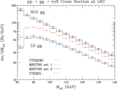
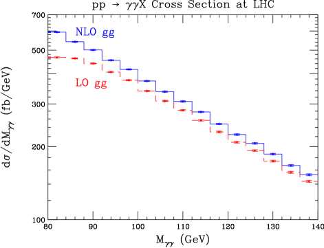
Figure 4: (a) Contribution of the gluon fusion subprocess to $pp\rightarrow\gamma\gamma X$ at the LHC, at leading order (lower four), and at NLO (upper three), using various parton distributions. (b) Total $pp\rightarrow\gamma\gamma X$ production at NLO, including NLO $q{\bar{q}}\rightarrow\gamma\gamma$ and fragmentation contributions, with the gluon fusion subprocess treated at LO (dashed) and at NLO (solid). MRST99 set 2 partons are used in (b). Contributions not involving gluon fusion into photons are obtained from DIPHOX. Both sets of plots are for $\mu_{R}=\mu_{F}=0.5M_{\gamma\gamma}$, and a standard photon isolation criterion with $R=0.4$, $E_{\rm T\,max}=15$ GeV. Statistical errors from numerical integration are shown.

Figure 4(a) shows the contribution of just the gluon fusion subprocess to $pp\rightarrow\gamma\gamma X$ at the LHC, at its leading and next-to-leading orders, for the standard cone photon isolation criterion with $R=0.4$, $E_{\rm T\,max}=15$ GeV, and for several choices of parton distributions. To help with comparisons to the results of ref. DIPHOX , we use MRST99 set 2 as our “default” choice. This set has a somewhat larger gluon distribution at large $x$ than MRST99 set 1, but the differences with this set, or with CTEQ5M1 CTEQ , at the smaller $x$ ranges probed here are small compared to the NLO corrections, or to the renormalization and factorization scale dependence, as we shall see. We also plot the LO cross section with the LO CTEQ5L distributions (using a LO $\alpha_{s}(m_{Z})=0.127$) CTEQ , in order to compare our NLO cross section with a “true” LO calculation. Recently, the more precise HERA data has been incorporated into two updated standard sets of distributions, MRST2001 MRST2001 and CTEQ6M CTEQ6M . However, neither set has a sizable change from its predecessor in the quark and gluon distributions for $x$ in the relevant range 0.01—0.1 at $Q^{2}=10^{4}$ GeV². The new MRST2001 distribution uses a slightly larger $\alpha_{s}(m_{Z})=0.119$, which may increase the importance of the gluon fusion subprocess relative to the $q\bar{q}$ subprocess by a few percent, but overall the effect on the $\gamma\gamma$ background should be fairly small.

Table 1: NLO QCD $K$ factors for $\gamma\gamma$ Higgs signal and gluon fusion background. Both LO and NLO cross sections are computed using NLO parton distributions.

$M_{\gamma\gamma}$ (GeV)	$K_{\rm Higgs}$	$K_{gg\rightarrow\gamma\gamma}$
98	2.92	1.82
118	2.54	1.61
138	2.39	1.55

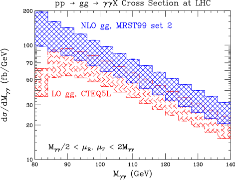
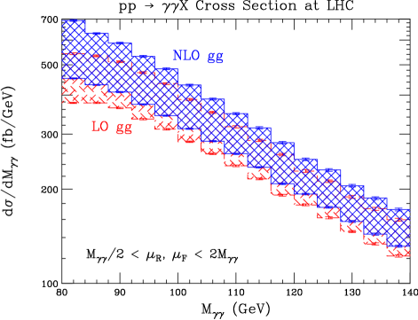
Figure 5: Scale dependence of (a) the gluon fusion subprocess contribution to $pp\rightarrow\gamma\gamma X$, and (b) the total $pp\rightarrow\gamma\gamma X$ production cross section, for standard photon isolation with $R=0.4$, $E_{\rm T\,max}=15$ GeV. In both plots, the bands represent the result of varying $\mu_{R}$ and $\mu_{F}$ over the square region $0.5M_{\gamma\gamma}<\mu_{R},\mu_{F}<2M_{\gamma\gamma}$. The dashed (solid) hatched band corresponds to including the gluon fusion subprocess at LO (NLO). For the leading order band in (a) only, the LO CTEQ5L parton distributions were used; otherwise the NLO MRST99 set 2 distributions were employed.

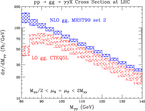
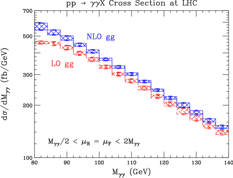
Figure 6: Scale dependence of (a) the gluon fusion subprocess contribution to $pp\rightarrow\gamma\gamma X$, and (b) the total $pp\rightarrow\gamma\gamma X$ production cross section. The cuts are identical to the ones in fig. 5. The parameters are identical to the ones used in the corresponding plots in fig. 5, except that the renormalization and factorization scales are set equal and varied between $0.5M_{\gamma\gamma}<\mu_{R}=\mu_{F}<2M_{\gamma\gamma}$.

In the absence of an NLO calculation, some experimental studies had used the $K$ factor (ratio of NLO over LO cross section) for Higgs production by gluon fusion as an estimate of the $K$ factor for $gg\rightarrow\gamma\gamma$. For example, $K_{\rm Higgs}^{\rm NLO}=1.85$ was used for a 100 GeV mass Higgs boson CMS . The reasoning is that both $gg\rightarrow H$ and $gg\rightarrow\gamma\gamma$ involve production of a colorless system from a gluon-gluon initial state. One difference between the two processes, however, is that the $Hgg$ coupling receives a fairly large short-distance renormalization NLOHiggs , from the top mass scale,

$$K_{\rm Higgs}^{\rm s.d.}\equiv 1+{11\over 2}{\alpha_{s}\over\pi}\approx 1.2,$$ (23)

which has no counterpart in the $gg\rightarrow\gamma\gamma$ correction. Another difference stems from the different loop momentum scales appearing in the real emission diagrams. For the $gg\rightarrow Hg$ case, the momentum in the loop is dominated by the heavy top quark mass, which is taken to be infinite in our calculation, while for the $gg\rightarrow\gamma\gamma g$ process the quarks in the loop are taken to be massless, so that the dominant momentum in the loop is that of the photons and the emitted gluon. As a result, the cross section for $gg\rightarrow\gamma\gamma g$ falls off more quickly with the emitted gluon transverse momentum than that for $gg\rightarrow Hg$, resulting in a smaller real-emission contribution to the total NLO cross section.

In comparing signal and background $K$ factors, it is of course useful to impose the same set of cuts on the photons in each case. In table 1 we list $K$ factors for both the $pp\rightarrow gg\rightarrow HX\rightarrow\gamma\gamma X$ Higgs production cross section and the $pp\rightarrow gg\rightarrow\gamma\gamma X$ gluon fusion background, for three representative choices of Higgs mass. (To be precise, the Higgs $K$ factor includes the subprocesses $qg\rightarrow Hq$ and $q\bar{q}\rightarrow Hg$ at NLO; removing them decreases $K_{\rm Higgs}$ by roughly 5% at $m_{H}=$ 118 GeV.) We take $\mu_{R}=\mu_{F}=0.5M_{\gamma\gamma}$ and impose the same photon acceptance and isolation cuts as in fig. 4(a), for both signal and background. (With both sets of cuts removed, each $K$ factor is about 10% smaller at $M_{\gamma\gamma}=$ 118 GeV, but their ratio is stable to a few percent.) We define the “LO cross section” entering the $K$ factor using NLO, rather than LO, parton distributions. This convention results in larger $K$ factors than the more standard convention, as can easily be seen by comparing the LO cross sections using the CTEQ5M1 and CTEQ5L distributions in fig. 4(a). In any case, the important point is that the $K$ factors for the gluon fusion component of the di-photon background are significantly smaller than the $K$ factors for the Higgs signal, even after accounting for the short-distance contribution (23) to the latter. This difference appears to be due to the relatively smaller real-emission contribution to the background.

In fig. 4(b) the effects of computing the gluon fusion subprocess at NLO are shown, for the total NLO $pp\rightarrow\gamma\gamma X$ production rate, i.e. including also the $q{\bar{q}}\rightarrow\gamma\gamma$ and fragmentation contributions at NLO obtained from DIPHOX DIPHOX . As in fig. 4(a), $\mu_{R}$ = $\mu_{F}=M_{\gamma\gamma}/2$ and the isolation criterion $R=0.4$, $E_{\rm T\,max}=15$ GeV is used. (The lower histogram in fig. 4(b), where the gluon fusion subprocess is treated at LO, corresponds to the result in fig. 13 of ref. DIPHOX , except that $R=0.4$, $E_{\rm T\,max}=5$ GeV is used in that plot.) The increase in the total irreducible $\gamma\gamma$ background which results from replacing the LO gluon fusion quark box by the NLO computation is a modest one, except at the lowest invariant masses relevant only for non-Standard-Model Higgs searches. In fig. 4(b), the increase ranges from 27% at $M_{\gamma\gamma}=82$ GeV, to 10% at 100 GeV, and only 6% at 138 GeV. For the most interesting mass range for the Higgs boson in this channel, 115 GeV $<m_{H}<$ 140 GeV, the overall effect on the square root of the background is under 5%. The larger increase at smaller $M_{\gamma\gamma}$ simply reflects the fact that the LO contribution vanishes, due to the kinematic cuts, as $M_{\gamma\gamma}\rightarrow 80$ GeV. This feature is seen most visibly in fig. 4(a).

In fig. 5, the dependence of the $\gamma\gamma$ background on the renormalization scale $\mu_{R}$ and factorization scale $\mu_{F}$ is illustrated by varying them independently over the square region $0.5M_{\gamma\gamma}<\mu_{R},\mu_{F}<2M_{\gamma\gamma}$. Figure 5(a) shows the variation for the gluon fusion subprocess contribution alone, while fig. 5(b) shows the variation for the total production rate, treating the $q{\bar{q}}\rightarrow\gamma\gamma$ and fragmentation contributions at NLO. The same photon isolation criterion is used as in fig. 4. In fig. 5(a), the leading-order (dashed hatched) band is computed using the LO parton distribution CTEQ5L, which is a bit more appropriate when considering this subprocess in isolation. In all cases, the maximum cross section in the band at a given $M_{\gamma\gamma}$ comes from setting $\mu_{R}=0.5M_{\gamma\gamma}$ and $\mu_{F}=2M_{\gamma\gamma}$, while the minimum cross section comes from setting $\mu_{R}=2M_{\gamma\gamma}$ and $\mu_{F}=0.5M_{\gamma\gamma}$. Allowing independent variations for $\mu_{R}$ and $\mu_{F}$ results in NLO bands which are not appreciably narrower than the LO bands. In contrast, varying $\mu_{R}$ and $\mu_{F}$ together, i.e. $\mu_{R}=\mu_{F}=\chi M_{\gamma\gamma}$ with $0.5<\chi<2$, as is more conventional, leads to much less scale variation for the gluon fusion subprocess at NLO than at LO, as shown in fig. 6. (These general features are also qualitatively present in the Higgs production cross section as well, although the larger NLO $K$ factor leads to stronger renormalization scale dependence in that case; see e.g. ref. CdFG .) The considerable improvement in the scale variation for the $gg$ contribution depicted in fig. 6(a) is diluted in fig. 6(b), where the contributions with quark initial states and fragmentation are added in.

In conclusion, the NLO corrections to the $gg\rightarrow\gamma\gamma$ subprocess have a modest effect on the total irreducible di-photon background to the Higgs search. Thus this subprocess can be considered to be under adequate theoretical control.

IV Statistical Significance of Higgs Signal

In this section we investigate the kinematic features of the Higgs signal and background, starting with photon isolation criteria. To facilitate this study we consider a crude approximation to an experimental analysis at the LHC. We assume a Higgs mass of 118 GeV, and we count the number of events in mass bins of 4 GeV for $30$ fb^-1 of integrated luminosity, corresponding to 3 years of running at low luminosity, ${\cal L}=10^{33}$cm^-2s^-1. We note that this choice of mass bin is slightly larger than the optimized mass bins of 2.74 and 3.44 GeV used in the ATLAS study of ref. Tisserand . We also include an efficiency factor of 0.57 for both signal and background, corresponding to the combination of 0.81 per $\gamma$ for $\gamma$/jet identification and 0.87 for fiducial cuts (mainly the transition between barrel and endcap) found in that analysis. Finally, we include a reducible background of 20% of the $\gamma\gamma$ continuum background, which we assume is possible after the $\gamma$/jet identification Tisserand . For this analysis we take the efficiency factors and the percentage of reducible background as independent of the isolation cuts; to investigate this further would require a more serious experimental analysis, beyond the scope of this work.

In computing the statistical significance we ignore interference between the Higgs signal and the background. In the Standard Model, the interference terms are on the order of a few percent of the Higgs signal gHgamInterf , and do not significantly alter any of our conclusions. The small size of the interference is due mostly to the extreme sharpness of the underlying Higgs resonance which, before smearing with the detector resolution, gives a peak in the cross section rising about a factor of a hundred over the background. Hence the interference contribution should not be more than about 20 percent of the signal. However, it is less than this because the primary Higgs production mode is via gluon fusion, so only the $gg\rightarrow\gamma\gamma$ component of the background can interfere. Also, because the experimental width is much greater than the intrinsic width, only the integral in $M_{\gamma\gamma}$ across the lineshape is observable. This integral vanishes unless there is a relative phase between the production ($gg\rightarrow H$), decay ($H\rightarrow\gamma\gamma$), and background ($gg\rightarrow\gamma\gamma$) amplitudes. The phase happens to vanish, up to small quark mass effects, when the background amplitude (for identical-helicity photons) is evaluated at one loop. The extra power of $\alpha_{s}$ in the two-loop amplitude then provides an additional suppression factor.

IV.1 Effects of varying photon isolation criteria

We first consider the effects on both signal and background of varying the photon isolation criteria, before turning in section IV.2 to the phenomenologically more viable method of using a jet veto to impose more stringent cuts. As mentioned in the introduction, photon isolation can be achieved by either a standard or a smooth cone criterion. In section III.2 we presented cross section results for the standard cone criterion with $R=0.4$ and $E_{\rm T\,max}=15$ GeV, values typical to previous analyses. Now we shall investigate how the $\gamma\gamma$ background varies, relative to the $H\rightarrow\gamma\gamma$ signal, as we change the isolation criteria. In particular, we would like to determine the parton-level statistical significance of the signal as a function of photon isolation.

Figure 7(a) shows how the $pp\rightarrow\gamma\gamma X$ production rate at the LHC depends on the parameters $R$ and $E_{\rm T\,max}$ of the standard cone isolation definition, while Figure 7(b) presents analogous information for the smooth cone criterion. As the isolation becomes more severe, i.e. $R$ is increased or $E_{\rm T\,max}$ or $\epsilon$ are decreased, the direct $pp\rightarrow\gamma\gamma X$ background becomes more suppressed. The large sensitivity to these parameters is indicative of the $q\gamma$ collinear singularity in the NLO $q\bar{q}\rightarrow\gamma\gamma X$ cross section. Since the QCD radiation in Higgs production has no such singularity, it should have no correlation with the photon directions, and therefore it should be less sensitive to the isolation criterion.

To see this more clearly, it is instructive to plot individually the various subprocess contributions to the $\gamma\gamma$ background. Figure 8(a) and (b), plotted for two different smooth cone isolation criteria, show how the $qg$ component is reduced relative to $q{\bar{q}}$ and $gg$ as the isolation requirement is made more severe. For instance, in the bin centered at $M_{\gamma\gamma}=118$ GeV, the $qg$ component decreases by 36%, in going from $R=0.4,\ \epsilon=1$ to $R=1,\ \epsilon=1$, while the $q{\bar{q}}$ and $gg$ components each only decrease by about 4%. The smooth cone criterion was used to simplify the discussion, since there are no fragmentation contributions; however, the results are qualitatively similar for the standard cone isolation.

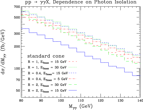
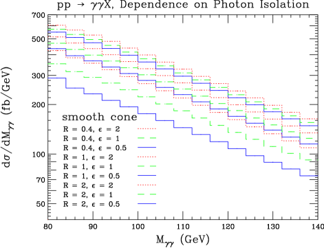
Figure 7: Dependence of $pp\rightarrow\gamma\gamma X$ at the LHC on photon isolation cuts, for (a) a set of standard cone isolation parameters, $R$ and $E_{\rm T\,max}$, and (b) a set of smooth cone isolation parameters, $R$ and $\epsilon$. All plots are for MRST99 set 2 partons, and $\mu_{R}=\mu_{F}=0.5M_{\gamma\gamma}$.

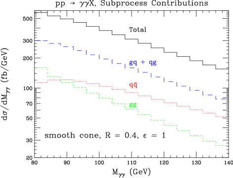
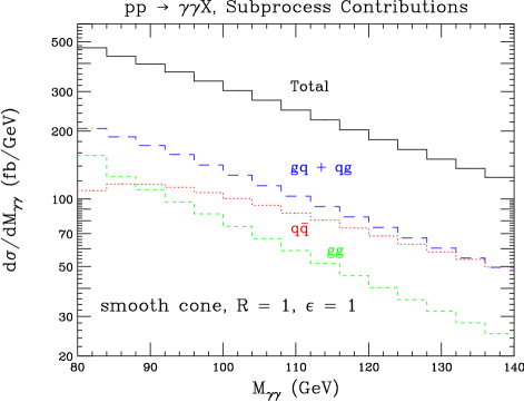
Figure 8: Contributions of the different subprocesses to $pp\rightarrow\gamma\gamma X$ at the LHC, as a function of di-photon invariant mass, for two choices of smooth cone isolation parameters: (a) $R=0.4$, $\epsilon=1$, and (b) $R=1$, $\epsilon=1$. The plots are computed at NLO, for MRST99 set 2 partons, with acceptance cuts (20), and $\mu_{R}=\mu_{F}=0.5M_{\gamma\gamma}$.

We give the number of Higgs signal ($S$) and background ($B$) events and the statistical significance ($S/\sqrt{B}$) in the bin 116 GeV $<M_{\gamma\gamma}<$ 120 GeV for the different choices of standard cone parameters in table 2, and for the choices of smooth cone parameters in table 3. For the standard cone, we find a statistical significance of 7.3 at $R=1,\ E_{\rm T\,max}=15$ GeV, for a modest gain of about 4% over the value of 7.0 at $R=0.4,\ E_{\rm T\,max}=15$ GeV. The significance can be increased further to 7.5 by the very severe cut of $R=2,\ E_{\rm T\,max}=15$ GeV, for a gain of 7% over the value at $R=0.4,\ E_{\rm T\,max}=15$ GeV. For the smooth cone, the statistical significance appears to have a maximum of about 7.4 for $R=1,\ \epsilon=0.5$ and $R=2,\ \epsilon=2$. It is clear from these results that for either the smooth or standard cones the statistical significance depends on the isolation cuts only rather weakly.

Table 2: Number of signal and background events and the statistical significance for $pp\rightarrow HX\rightarrow\gamma\gamma X$ in a bin 116 GeV $<M_{\gamma\gamma}<$ 120 GeV for $30$ fb^-1 integrated luminosity using standard cone isolation. The Higgs mass is taken to be $m_{H}=$ 118 GeV. Other experimental assumptions are given in the text.

$(R,E_{\rm T\,max}$ in GeV)	$S$	$B$	$S/\sqrt{B}$
(0.4,15)	993	20,400	7.0
(0.4,5)	980	19,000	7.1
(1,30)	979	20,600	6.8
(1,15)	952	16,900	7.3
(2,30)	896	16,400	7.0
(2,15)	789	11,000	7.5

Table 3: Number of signal and background events and the statistical significance for $pp\rightarrow HX\rightarrow\gamma\gamma X$ in a bin 116 GeV $<M_{\gamma\gamma}<$ 120 GeV for $30$ fb^-1 integrated luminosity using smooth cone isolation. The Higgs mass is taken to be $m_{H}=$ 118 GeV. Other experimental assumptions are given in the text.

$(R,\epsilon)$	$S$	$B$	$S/\sqrt{B}$
(0.4,2)	993	22,000	6.7
(0.4,1)	992	20,800	6.9
(0.4,0.5)	985	20,000	7.0
(1,2)	969	18,100	7.2
(1,1)	948	16,700	7.3
(1,.5)	915	15,400	7.4
(2,2)	893	14,700	7.4
(2,1)	806	12,300	7.3
(2,.5)	685	9,800	6.9

The smallest cone size, $R=0.4$, used in tables 2 and 3, is the standard cone size used in previous studies. Recently it was observed CataniPhotons that logarithms of the form $\alpha_{s}(\mu)\ln(1/R^{2})$ GV can invalidate an NLO calculation of prompt photon production: For $R=0.1$ the NLO single-photon cross section with isolation was larger than the cross section with no isolation, which is clearly an unphysical result. It is not yet known precisely how small $R$ can be taken before the NLO calculation begins to break down. However, for $R=0.4$, the $\ln(1/R^{2})$ factor is 2.5 times smaller than it is for the pathological case of $R=0.1$. Also, the physical scale in the di-photon invariant masses relevant for the LHC Higgs search is significantly higher than the single-photon $p_{\rm T}(\gamma)=15$ GeV case studied in ref. CataniPhotons , rendering $\alpha_{s}(\mu)$ smaller as well. Finally, we note that the large logarithms do not arise from the gluon fusion contributions, because there is no $g\gamma$ collinear singularity. Hence the effect of the logarithms in the single-photon case (where gluon fusion is not important and was not included) is diluted somewhat in the di-photon case by the gluon fusion contribution. Nevertheless, further study of this situation, including possibly resummation of the logarithms, could be helpful.

A more critical issue for this analysis is that the most severe isolation parameters may not be phenomenologically viable, for both the theoretical and experimental reasons mentioned in the introduction. Theoretically, it is not infrared safe to forbid all gluon radiation into any finite region of phase space. If the isolation criteria approach this limit, the perturbative predictions become subject to large corrections and therefore become unreliable GV ; CataniPhotons . After all, two $R=2$ cones can cover most of the $(\eta,\phi)$ plane within the detector acceptance, and $E_{\rm T\,max}=15$ GeV is not a lot of energy at the LHC. On the experimental side, the efficiency for collecting signal events may decline for reasons that are absent from the NLO Monte Carlo. Instrumental (calorimeter) noise, pile up, and energy deposition from the underlying event plus overlapping minimum bias collisions, all contribute an average energy in a cone which scales roughly as the area of the cone. Thus one might expect that when $R$ is increased, one should also increase $E_{\rm T\,max}$, roughly like $R^{2}$. For the $R=0.4$ cone typically used, pile up and underlying events start to saturate the cone at $E_{\rm T\,max}\approx 2.5$ GeV DIPHOX ; Wielers . For $R=2$, saturation would most likely be occurring at $E_{\rm T\,max}=15$ GeV, perhaps even at 30 GeV. Another potential problem is that as one varies the cuts to reduce the irreducible contributions, one must be sure that the reducible contributions do not get larger, undoing the improvement. For example, we have raised the total transverse energy allowed near the photon, in going from $R=0.4$, $E_{\rm T\,max}=15$ GeV to, say, $R=2$, $E_{\rm T\,max}=30$ GeV, and this may allow more of the reducible background to enter. This question could be addressed by studies along the lines of ref. PiBkgd . In any case, it is clear that a phenomenologically more sensible method for rejecting events with hadronic energy near the photons is required.

IV.2 Jet veto

As mentioned in the introduction, a veto on nearby jets offers another way to suppress the QCD background, in particular the $qg\rightarrow\gamma\gamma q$ process Tisserand . At the NLO parton level, at least for direct processes, it corresponds closely to increasing the size of the cone. However, because transverse energy is being forbidden into a smaller area (the jet cone size), for the same amount of suppression at NLO, the jet veto is a more infrared safe criterion, and it should also have better experimental properties (less loss of signal due to noise, overlapping events, etc.).

Jet vetoes have been considered previously in search strategies for other Higgs decay modes, particularly $H\rightarrow W^{+}W^{-}\rightarrow e^{\pm}\mu^{\mp}/{\hbox{\kern-6.0pt$p_{\rm T}$}}$ RunIIExpectations ; CMS2 ; ATLAS ; DD ; HanZhangCdFG . In those cases, typically a general veto is applied on all jets in the detector acceptance with $E_{T}$ above a certain value. For the $\gamma\gamma$ mode, we would only like to veto on jets “close” to the photon candidates. Such nearby jets are more likely to come from the $qg\rightarrow\gamma\gamma q$ subprocess, because of the final state $q\gamma$ collinear singularity, than from the Higgs production process $gg\rightarrow HX$. On the other hand, because the gluon is in a larger color representation than the quark, $gg$-initiated production of a color singlet object tends to be jettier overall than production initiated by $q\bar{q}$ or $qg$ initial states. In fact, cuts requiring a minimum transverse momentum of the $\gamma\gamma$ pair, $Q_{T}>30$ GeV, have been proposed to take advantage of this fact Abdullin ; GGGamGamGa ; GGGamGamGb , and enhance the signal. So only jets “sufficiently” near a photon candidate should be vetoed.

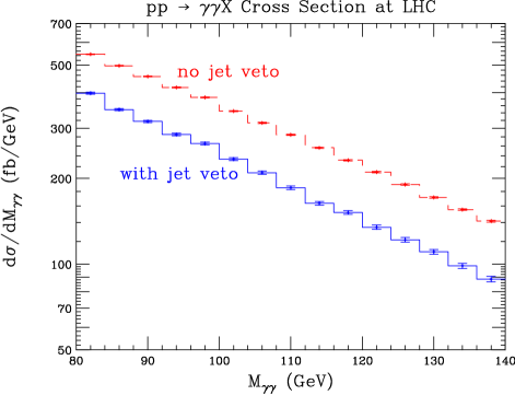
Figure 9: Effect on the background process $pp\rightarrow\gamma\gamma X$ of vetoing on jets with $E_{\rm T}>15$ GeV within $R_{\rm jet}=2$ of either photon candidate. The veto is on top of standard cone isolation with $R=0.4$, $E_{\rm T\,max}=5$ GeV. MRST99 set 2 partons are used, with the default acceptance cuts (20) and scale choice (22).

We implement the jet veto on top of a standard photon isolation cone, represented by the inner cone in fig. 3. We require that there is no jet with a transverse energy $E_{\rm T}>E_{\rm T\,jet}$ within a radius $R_{\rm jet}$ of the photon, represented by the outer cone in fig. 3. We do not include hadronic energy inside the inner cone in defining this jet. Then the results at the NLO parton level do not depend on the cone size $R^{\rm cone}_{\rm jet}$ used in the jet algorithm, but for definiteness we suppose $R^{\rm cone}_{\rm jet}=0.7$.

As an example of the jet veto suppression, Figure 9 shows the background suppression obtained for a jet veto using $R_{\rm jet}=2$ and $E_{\rm T\,jet}=15$ GeV on top of a standard isolation cone with $R=0.4$ and $E_{\rm T\,max}=5$ GeV. For this standard isolation cone the fragmentation contribution is rather small, amounting to about 10 percent of the total. This simplifies the calculation of the jet veto since we can ignore the action of the jet veto on the small fragmentation part. For the direct piece at NLO, a jet to be vetoed amounts to a lone parton with transverse energy $E_{T}>E_{\rm T\,jet}=15$ GeV between the inner and outer cones $0.4<R<2$. By ignoring the jet veto rejection of the fragmentation term, the background is overestimated by a few percent. In this approximation, with $m_{H}=118$ GeV, the bin 116 GeV $<M_{\gamma\gamma}<$ 120 GeV has 776 signal events and 12,600 background events, leading to a statistical significance of $S/\sqrt{B}=6.9$. Even though the background drops from 19,000 events for the standard isolation case with $R=0.4$ and $E_{\rm T\,max}=5$ GeV to 12,600 events when the jet veto is included, the statistical significance is essentially unchanged compared to this case. This illustrates the rather disappointing insensitivity of the statistical significance to the presence of the jet veto.

IV.3 Kinematic distributions of signal and background photons

The situation can be improved somewhat by including information from the photon angular distribution. Since the Higgs boson is a scalar, its decay to two photons is isotropic in its rest frame. In contrast, the $\gamma\gamma$ background processes tend to be more peaked toward the beam axis. Thus, the angular distribution of the photons can help separate the signal from the background.

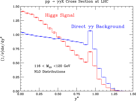
Figure 10: The angular distribution as a function of $y^{*}$ for 116 GeV $<M_{\gamma\gamma}<$ 120 GeV. The renormalization and factorization scales are $\mu_{R}=\mu_{F}=0.5M_{\gamma\gamma}$ and the smooth cone isolation cuts are $R=1,\epsilon=1$. The Higgs mass is taken to be $m_{H}=118$ GeV. The peaks near $y^{*}=0.94$ occur in a region where the NLO calculation breaks down and is not trustworthy.

Figure 10 shows the normalized distribution in the di-photon rapidity difference, $y^{*}=(y(\gamma_{1})-y(\gamma_{2}))/2$. This variable is convenient because it is simple to determine experimentally, and at lowest order it is related to the center-of-mass scattering angle $\theta^{*}$ for $q\bar{q}\rightarrow\gamma\gamma$ or $gg\rightarrow\gamma\gamma$ by $\cos\theta^{*}=\tanh y^{*}$. The renormalization and factorization scales are set to our default values (22), and only events in the mass bin 116 GeV $<M_{\gamma\gamma}<$ 120 GeV are kept. The smooth cone isolation is used with parameters $R=1$ and $\epsilon=1$; similar distributions are obtained using a standard cone isolation. As can be seen in fig. 10 the angular distribution of the Higgs signal events is rather different from the background. We can estimate the significance that could be obtained by using a maximum likelihood function with this information to be

$$\left(\sum_{i}{S^{2}_{i}\over B_{i}}\right)^{1/2}=7.7\ ,$$ (24)

where the sum is over the bins in $y^{*}$. This number is to be compared with a significance of

$${\sum_{i}S_{i}\over(\sum_{i}B_{i})^{1/2}}=7.3\ ,$$ (25)

without using the angular information. The 4% relative improvement in significance should also hold roughly for $y^{*}$ distributions constructed using a standard cone isolation.

An interesting feature in fig. 10 are the peaks in both the signal and background in the bins near 0.90-1.00. These peaks are attributable to a breakdown of the NLO approximation near the LO kinematic boundary in $y^{*}$, whose location is dictated by the $p_{T}(\gamma_{1})>40$ GeV cut (20) and $M_{\gamma\gamma}\approx 118$ GeV. At LO the two photons are constrained to have vanishing total transverse momentum $Q_{T}\equiv|\vec{p}_{1\rm T}+\vec{p}_{2\rm T}|$, which leads to $y^{*}<0.94$. At NLO, events with a radiated gluon can have nonzero $Q_{T}$, which removes the constraint on $y^{*}$. For small $Q_{T}$, the NLO cross section is very unstable and must be resummed in $\alpha_{s}\ln^{2}(Q_{T}/p_{T})$, as in refs. GGGamGamGb ; BY . Similar phenomena have been described in earlier work on isolated photons IsolatedPhotonIR ; DIPHOX . A general description of such “edges” has also been given CataniWebber . In fig. 10, $\ln(Q_{T}/p_{T})$ becomes appreciable only in the two bins centered at $y^{*}=0.93$ and $0.99$. The bins to the left of $y^{*}=0.94$ do not contain these uncancelled logarithms because the virtual corrections, with LO kinematics, can contribute and cancel them. Of course, all bins to the right of $y^{*}=0.94$ are effectively being calculated at LO, hence their overall normalization is not as trustworthy.

One might be concerned that the parton-level normalized distributions shown in fig. 10 will be distorted by higher-order terms, soft physics, and detector effects, rendering the information inadequate for improving the significance of the signal. However, this is not the case, because 1) only an approximate knowledge of the relative shapes of signal and background is required to get most of the benefit, and 2) the background distribution can be measured experimentally. Once a putative peak is identified in the $M_{\gamma\gamma}$ spectrum, the $y^{*}$ distribution in the sideband regions above and below the peak can be measured. This information, along with that in fig. 10, can be used to estimate the true signal distribution, including detector effects, etc. One can then apply an optimal observable or maximum likelihood analysis similar to the one described above.

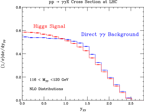
Figure 11: The signal and background distributions as a function of $y_{\gamma\gamma}$ for 116 GeV $<M_{\gamma\gamma}<$ 120 GeV. The renormalization and factorization scales are $\mu_{R}=\mu_{F}=0.5M_{\gamma\gamma}$ and the smooth cone isolation cuts are $R=1,\epsilon=1$. The Higgs mass is taken to be $m_{H}=118$ GeV.

The final distribution that we consider is that of $y_{\gamma\gamma}$, defined to be the rapidity of $p_{\gamma\gamma}=p_{\gamma_{1}}+p_{\gamma_{2}}$, the four-vector sum of the two photon momenta. For the case of the Higgs signal, this is just the rapidity of the Higgs boson. We plot the normalized distribution in $y_{\gamma\gamma}$ in Figure 11, for the same choice of mass bin, isolation cuts, and scale choices as for Figure 10. The difference between the signal and the background distributions can be mostly attributed to the different parton luminosities involved in the production; the Higgs signal is produced by a predominantly $gg$ initial state, whereas the di-photon background gets significant contributions from each of $q\bar{q}$, $qg$, and $gg$. In this case the use of $y_{\gamma\gamma}$ in a maximum likelihood function analysis would improve the significance by less than a percent.

V Conclusions and outlook

In this paper we presented a next-to-leading order study of the irreducible di-photon background, including the corrections to the gluon fusion subprocess $gg\rightarrow\gamma\gamma$. The NLO gluon fusion is the largest of the higher order contributions not included in previous studies TwoPhotonBkgd1 ; DIPHOX . The scale dependence of the gluon-fusion contribution at NLO is roughly the same as at LO if the renormalization and factorization scales are varied independently, but is significantly reduced if they are varied in unison. Moreover, the NLO corrections to the gluon-fusion component, as a contribution to the total irreducible background, were found to be modest, suggesting that this calculation is under adequate theoretical control. Indeed, the NLO $K$ factor for the $gg\rightarrow\gamma\gamma$ subprocess is only about 65% of the NLO $K$ factor for Higgs production. Experimental studies using the latter $K$ factor to estimate the former one CMS have therefore been a bit too conservative.

Using the improved calculation we investigated the statistical significance of Higgs production as a function of the photon isolation cuts. We found that the significance depends only weakly on the isolation cuts. Although we found a slight enhancement with more severe cuts, we noted that as isolation becomes tight, instrumental noise, soft hadrons and overlapping events can render the cuts experimentally unworkable. Moreover, the perturbative predictions become subject to large corrections and are unreliable. A better procedure is to include a veto on jets near the photon candidates. This can suppress the background without suffering from the drawbacks of tight photon isolation. As an example, we computed the extra suppression due to a jet veto when the effects of fragmentation can be neglected. We found that although the background is suppressed, the statistical significance is hardly altered. More generally one would need to also include a jet veto on the fragmentation contribution, but only a weak dependence may be anticipated. The most robust improvement we found in the statistical significance of the Higgs signal, albeit still modest, was obtained using the rapidity difference $y^{*}$ distribution of the decay photons. It would be interesting to explore other variables characterizing the distribution of hadronic energy in the events; a strategy which optimizes the use of this information without cutting out large numbers of events may be possible.

These results would need to be investigated further in a more realistic simulation than just the parton-level one we have done here. In particular, the effects of instrumental noise and overlapping events must be included Wielers . One would also need to include a detailed study of the reducible $\pi^{0}$ background contributions Tisserand ; Wielers ; PiBkgd . Once a more realistic study is set up, the entire range up to $m_{H}<140$ GeV would need to be investigated, instead of just the single choice of $m_{H}=118$ GeV used in section IV.3. When the LHC di-photon data becomes available, the information provided by the sideband regions will also be crucial.

As described in the introduction, there are a number of ${\cal O}(\alpha_{s}^{2})$ contributions that still have not been included. These corrections are all expected to be smaller than the ${\cal O}(\alpha_{s}^{3})$ gluon fusion contribution incorporated into the computation presented here. Nevertheless, for completeness as well as to confirm that there are no surprises, it would be useful to evaluate all remaining ${\cal O}(\alpha_{s}^{2})$ contributions. It would also be useful to incorporate a resummation of the large logarithms which appear at the kinematic edges of angular distributions CataniWebber and for small cone sizes GV ; CataniPhotons .

We are hopeful that further studies will lead to a better understanding of the di-photon background, and to an increased sensitivity for the Higgs search at the LHC.