IFT-02-10 UCD-02-08 DFF-385-03-02 hep-ph/0206192

The Scalar Sector of the Randall-Sundrum Model

Daniele DOMINICI${}^{\>1),\>}$ Bohdan GRZADKOWSKI${}^{\>2),\>}$
John F. GUNION${}^{\>3),\>}$ Manuel TOHARIA${}^{\>3),\>}$

ABSTRACT

We consider the scalar sector of the Randall-Sundrum model. We derive the effective potential for the Standard Model Higgs-boson sector interacting with Kaluza-Klein excitations of the graviton ($h_{\mu}^{\nu\,n}$) and the radion ($\phi$) and show that only the Standard Model vacuum solution of $\partial V(h)/\partial h=0$ ($h$ is the Higgs field) is allowed. We then turn to our main focus: the consequences of the curvature-scalar mixing $\xi\,R\,\widehat{H}^{\dagger}\widehat{H}$ (where $\widehat{H}$ is a Higgs doublet field on the visible brane), which causes the physical mass eigenstates $h$ and $\phi$ to be mixtures of the original Higgs and radion fields. First, we discuss the theoretical constraints on the allowed parameter space. Next, we give precise procedures for computing the $h$ and $\phi$ couplings given the physical eigenstate masses, $m_{h}$ and $m_{\phi}$, $\xi$ and the new physics scales of the model. Relations among these new-physics scales are discussed and a set of values not far above the smallest values required by precision electroweak constraints and RunI data is chosen. A simple result for the sum of the $ZZh$ and $ZZ\phi$ squared couplings relative to the $ZZh_{SM}$ squared coupling is derived. We demonstrate that this sum rule in combination with LEP/LEP2 data implies that not both the $h$ and $\phi$ can be light. We present explicit results for the still allowed region in the $(m_{h},m_{\phi})$ plane that remains after imposing the appropriate LEP/LEP2 upper limits coming from the Higgs-strahlung channel. In the remaining allowed region of parameter space, we examine numerically the couplings and branching ratios of the $h$ and $\phi$ for several cases with $m_{h}=120\;\hbox{GeV}$ and $m_{\phi}\leq 300\;\hbox{GeV}$. The resulting prospects for detection of the $h$ and $\phi$ at the LHC, a future LC and a $\gamma\gamma$ collider are reviewed. For moderate $|\xi|$, both the anomalous $h\to gg$ coupling and (when $m_{h}>2m_{\phi}$) the non-standard decay channel $h\to\phi\phi$ can substantially impact $h$ discovery. Presence of the latter is a direct signature for non-zero $\xi$. We find that $BR(h\to\phi\phi)$ as large as $30\div 40\,\%$ is possible when $|\xi|$ is large. Conversely, if $m_{\phi}>2m_{h}$ then $BR(\phi\to hh)$ is generally large. Detection of a light $\phi$ might require the LC. Detection of a heavy $\phi$ might need to take into account the $\phi\to hh$ channel. The feasibility of experimentally measuring the anomalous $gg$ and $\gamma\gamma$ couplings of the $h$ and $\phi$ is examined.

PACS: 04.50.+h, 12.60.Fr

Keywords: extra dimensions, Higgs-boson sector, Randall-Sundrum model

1 Introduction

The Standard Model (SM) of electroweak interactions describes successfully almost all existing experimental data. However the model suffers from many theoretical drawbacks. One of these is the hierarchy problem: namely, the SM can not consistently accommodate the weak energy scale ${\cal O}(1\;\hbox{TeV})$ and a much higher scale such as the Planck mass scale ${\cal O}(10^{19}\;\hbox{GeV})$. Therefore, it is commonly believed that the SM is only an effective theory emerging as the low-energy limit of some more fundamental high-scale theory that presumably could contain gravitational interactions. In the last few years there have been many models proposed that involve extra dimensions. These models have received tremendous attention since they could provide a solution to the hierarchy problem. One of the most attractive attempts has been formulated by Randall and Sundrum [1], who postulated a 5D universe with two 4D surfaces (“3-branes”). In the simplest version, all the SM particles and forces with the exception of gravity are assumed to be confined to one of the 3-branes called the visible brane. Gravity lives on the visible brane, on the second brane (the “hidden brane”) and in the bulk. All mass scales in the 5D theory are of the order of the Planck mass. By placing the SM fields on the visible brane, all the order Planck mass terms are rescaled by an exponential suppression factor (the “warp factor”) $\Omega_{0}\equiv e^{-m_{0}b_{0}/2}$, which reduces them down to the weak scale ${\cal O}(1\;\hbox{TeV})$ on the visible brane without any severe fine tuning. A ratio of $1\;\hbox{TeV}/M_{Pl}$ (where $M_{Pl}$ is the reduced Planck mass, $M_{Pl}\sim 2.4\times 10^{18}\;\hbox{GeV}$) corresponds to $m_{0}b_{0}/2\sim 35$. This is a great improvement compared to the original problem of accommodating both the weak and the Planck scale within a single theory.

In order to obtain a consistent solution to the Einstein equations corresponding to a low-energy effective theory on the visible brane with a flat metric, the branes must have equal but opposite cosmological constants and these must be precisely related to the bulk cosmological constant. The model is defined by the 5D action:

$$S = -\int d^{4}x\,dy\sqrt{-\widehat{g}}\left({R\over 16\pi G_{5}}+\Lambda\right)$$ (1)

$$+\int d^{4}x\,\sqrt{-g_{hid}}({\cal L}_{hid}-V_{hid})+\int d^{4}x\,\sqrt{-g_{vis}}({\cal L}_{vis}-V_{vis}),$$

where $\widehat{g}^{\widehat{\mu}\widehat{\nu}}$ ($\widehat{\mu},\widehat{\nu}=0,1,2,3,4$, where $4$ refers to the $y$ coordinate) is the bulk metric and $g_{hid}^{\mu\nu}(x)\equiv\widehat{g}^{\mu\nu}(x,y=0)$ and $g_{vis}^{\mu\nu}(x)\equiv\widehat{g}^{\mu\nu}(x,y=1/2)$ ($\mu,\nu=0,1,2,3$) are the induced metrics on the branes. We will use the notation $\epsilon^{2}=16\pi G_{5}=1/M_{Pl\,5}^{3}$.  One finds that if the bulk and brane cosmological constants are related by $\Lambda/m_{0}=-V_{hid}=V_{vis}=-12m_{0}/\epsilon^{2}$ and if periodic boundary conditions identifying $(x,y)$ with $(x,-y)$ are imposed, then the 5D Einstein equations lead to the following metric:

$$ds^{2}=e^{-2\sigma(y)}\eta_{\mu\nu}dx^{\mu}dx^{\nu}-b_{0}^{2}dy^{2},$$ (2)

where $\sigma(y)=m_{0}b_{0}\left[y(2\theta(y)-1)-2(y-1/2)\theta(y-1/2)\right]$; $b_{0}$ is a constant parameter that is not determined by the action, Eq. (1). Gravitational fluctuations around the above background metric will be defined through the replacements:

$$\eta_{\mu\nu}\to\eta_{\mu\nu}+\epsilon h_{\mu\nu}(x,y)\;\;\;\;\;\;b_{0}\to b_{0}+b(x)\,.$$ (3)

Below we will be expanding in powers of $\epsilon h_{\mu\nu}$ and eventually $b(x)/b_{0}$ as well.

The paper is organized as follows. First, in Sec. 2 we describe the basic framework for our analysis and derive the effective potential for the SM Higgs-boson sector interacting with Kaluza-Klein excitations of the graviton ($h_{\mu}^{\nu\,n}$) and the radion ($\phi$). We discuss the need to retain a full form in order to show that the only consistent minimum of this effective potential is the standard one. In Sec. 3, we introduce the the curvature-scalar mixing $\xi\,R\,\widehat{H}^{\dagger}\widehat{H}$ and discuss its consequences for couplings and interactions. Here, $\widehat{H}$ is the Higgs field on the visible brane before any rescalings required for canonical normalization. In Sec. 4, we detail the phenomenology of the scalar sector, including the particularly important possibility of $h\to\phi\phi$ decays, assuming that the new physics scale is large, $\Lambda_{\phi}=5\;\hbox{TeV}$ (where $\Lambda_{\phi}$ specifies the strength of the radion interactions with matter). We consider detection of the $h$ and $\phi$ at both the Large Hadron Collider (LHC) and a future linear collider (LC), as well as in $\gamma\gamma$ collisions at the latter. In Sec. 5, we discuss the even more dramatic features that would arise if $\Lambda_{\phi}=1\;\hbox{TeV}$, a choice that might be excluded with additional analysis of RunI Tevatron data and/or precision electroweak constraints. We summarize our results in Sec. 6. The Appendix presents a complete tabulation of the Feynman rules we employ.

There is already an extensive literature on the scalar sector phenomenology of the Randall-Sundrum model. Studies in the absence of mixing ($\xi=0$) include Refs. [3, 4, 5, 6, 7]. Some aspects of $\xi\neq 0$ phenomenology appear in Refs. [8, 9, 10, 11]. In this paper, we focus especially on the impacts of the tri-linear couplings that emerge only when $\xi\neq 0$ mixing is present.

2 The effective potential

Our first goal is to determine the effective potential that is defined as a collection of all non-derivative contributions to the 4D effective Lagrangian density. We wish to demonstrate that the the standard vacuum defined by the stationary point of the Higgs potential is the unique potential minimum. It turns out that this requires using a very complete form for the full effective potential.

In order to show that standard 4D gravity is reproduced by the model, and to identify scalar degrees of freedom related to fluctuations of $b_{0}$, let us assume temporarily that $h_{\mu\nu}$ is only a function of $x$. Integrating the bulk Lagrangian over the 5-th dimension one finds a contribution to the effective action (see, for example, [2]):

$$S_{eff}=\int d^{4}x\,\sqrt{-g}\left(-{(1-\Omega_{b}^{2})\over\epsilon^{2}m_{0}}\,R^{(4)}(g)+{6\over\epsilon^{2}m_{0}}\,(\partial_{\mu}\Omega_{b})\,(\partial^{\mu}\Omega_{b})+\cdots\right)$$ (4)

where $g_{\mu\nu}(x)$ denotes the $\eta_{\mu\nu}+\epsilon h_{\mu\nu}$ part of the metric, $R^{(4)}(g)$ is the 4D Ricci scalar and $\Omega_{b}(x)\equiv e^{-m_{0}[b_{0}+b(x)]/2}$. Standard 4D gravity is reproduced by requiring

$${M_{Pl}^{2}\over 2}={1-\Omega_{0}^{2}\over\epsilon^{2}m_{0}}.$$ (5)

where $\Omega_{0}\equiv e^{-m_{0}b_{0}/2}$ is known as the warp factor and $M_{Pl}\sim 2.4\times 10^{18}\;\hbox{GeV}$ is the reduced Planck mass defined as $1/\sqrt{8\pi G_{4}}$. The canonically normalized massless radion field $\phi_{0}(x)$ is defined by:

$$\phi_{0}(x)\equiv\left({12\over\epsilon^{2}m_{0}}\right)^{1/2}\Omega_{b}(x)\simeq\sqrt{6}M_{Pl}\Omega_{b}(x)\,.$$ (6)

For the Lagrangian of Eq. (4), the radion is massless and there is no potential leading to a definite vacuum expectation value for the radion field. This result is already apparent at the level of the RS solution of the Einstein equations, Eq. (2), where $b_{0}$ appeared as a free parameter. Therefore, some potential, $V(\phi_{0})$, for the radion field is necessary [12] in order to determine its vacuum expectation value and in consequence stabilize the distance between the branes: $\langle\phi_{0}\rangle\equiv\Lambda_{\phi}=\sqrt{6}M_{Pl}\Omega_{0}$.

The SM action for the Higgs doublet $\widehat{H}$ on the visible brane is

$$S_{vis}\equiv\int d^{4}x\,\sqrt{-g_{vis}}({\cal L}_{vis}-V_{vis})=\int d^{4}x\sqrt{-g}\left[\Omega_{b}^{2}D_{\mu}\widehat{H}^{\dagger}D^{\mu}\widehat{H}-\Omega_{b}^{4}V(\widehat{H})\right],$$

where we will show that $V(\widehat{H})$ must vanish at the potential minimum, implying $V(\widehat{H})=\lambda\left(\widehat{H}^{\dagger}\widehat{H}-{\textstyle{1\over 2}}\hat{v}^{2}\right)^{2}$, and in the first term the $\Omega_{b}^{4}$ from $\sqrt{-g_{vis}}$ is partially canceled by the $\Omega_{b}^{-2}$ from $g_{vis}$ in $g_{vis}^{\mu\nu}\partial_{\mu}\widehat{H}^{\dagger}\partial_{\nu}\widehat{H}$. (In the final form of Eq. (2) and in subsequent equations the flat metric $\eta_{\mu\nu}$ will be assumed whenever repeated indices are summed.)

Incorporating $\Omega_{0}$ into the definition of the Higgs doublet by the rescaling $H_{0}\equiv\Omega_{0}\widehat{H}$, and employing the radion field $\phi_{0}$ of Eq. (6), we can rewrite $S_{vis}$ as

$$S_{vis}=\int d^{4}x\sqrt{-g}\left[\left({\phi_{0}\over\Lambda_{\phi}}\right)^{2}D_{\mu}H_{0}^{\dagger}D^{\mu}H_{0}-\left({\phi_{0}\over\Lambda_{\phi}}\right)^{4}V(H_{0})\right],$$ (7)

where the above form of $V(\widehat{H})$ implies that $V(H_{0})=\lambda\left(H_{0}^{\dagger}H_{0}-{\textstyle{1\over 2}}v_{0}^{2}\right)^{2}$ with $v_{0}\equiv\Omega_{0}\widehat{v}$. Expanding around the (presumed) vacuum expectation values for the radion, $\phi_{0}\to\Lambda_{\phi}+\phi_{0}$, and for the Higgs-boson, $H_{0}\to{1\over\sqrt{2}}(v_{0}+h_{0}+ia_{0})$, and dropping terms involving the Goldstone boson $a_{0}$, one gets the following contribution to the effective action involving $\phi_{0}$ and $h_{0}$:

$$\int d^{4}x\sqrt{-g}\left\{{\cal L}^{SM}(h_{0})-{\phi_{0}\over\Lambda_{\phi}}T_{\mu}^{\mu}(h_{0})+\left({\phi_{0}\over\Lambda_{\phi}}\right)^{2}\left[{\textstyle{1\over 2}}\partial_{\mu}h_{0}\partial^{\mu}h_{0}-6V(h_{0})\right]+{\cal O}\left[\left({\phi_{0}\over\Lambda_{\phi}}\right)^{3}\right]\right\},$$ (8)

where ${\cal L}^{SM}(h_{0})$ denotes the SM piece, $T_{\mu}^{\mu}(h_{0})=4V(h_{0})-\partial_{\mu}h_{0}\partial^{\mu}h_{0}$ and the form of $V(h_{0})$ corresponding to the above $V(H_{0})$ is

$$V(h_{0})=\lambda\left(v_{0}h_{0}+{h_{0}^{2}\over 2}\right)^{2}\,.$$ (9)

That $V(h_{0})$ must indeed vanish as $h_{0}\to 0$ will be shown shortly.

From the form of the rescaled potential $V(h_{0})$ in Eq. (9), it is clear that even if the typical scale of the 5D theory is of the order of the reduced Planck scale, $\widehat{v}\sim M_{Pl}$, then $v_{0}=e^{-m_{0}b_{0}/2}\widehat{v}\sim 1\;\hbox{TeV}$ for moderate values of model parameters: $m_{0}b_{0}/2\sim 35$. Therefore, the existence of the warp factor provides a solution to the hierarchy problem, as it explains the large ratio of $M_{Pl}/1\;\hbox{TeV}$.

Keeping in mind that $h_{\mu\nu}(x,y)$ depends both on $x$ and $y$, we use the KK expansion in the extra dimension

$$h_{\mu\nu}(x,y)=\sum_{n}h_{\mu\nu}^{n}(x){\chi^{n}(y)\over\sqrt{b}_{0}}$$ (10)

on the visible brane ($y=1/2$) to obtain

$$\sqrt{-g} = 1+{\epsilon\over 2}h_{\rho}^{\rho}-{\epsilon^{2}\over 4}\left(h_{\sigma}^{\rho}h_{\rho}^{\sigma}-{1\over 2}h_{\rho}^{\rho}h_{\sigma}^{\sigma}\right)+\mathcal{O}(\epsilon^{3})$$

$$= 1+{1\over\widehat{\Lambda}_{W}}\sum_{n}h_{\rho}^{\rho\,n}-\left({1\over\widehat{\Lambda}_{W}}\right)^{2}\sum_{n,m}\left(h_{\sigma}^{\rho\,n}h_{\rho}^{\sigma\,m}-{\textstyle{1\over 2}}h_{\rho}^{\rho\,n}h_{\sigma}^{\sigma\,m}\right)+{\cal O}\left[\left({h^{n}\over\widehat{\Lambda}_{W}}\right)^{3}\right]\,,$$

where

$$\widehat{\Lambda}_{W}\equiv{2\sqrt{b_{0}}\over\epsilon\chi^{n}(1/2)}\sim\sqrt{2}M_{Pl}\Omega_{0}\,,$$ (12)

where we used $\chi^{n}(1/2)\sim\sqrt{m_{0}b_{0}}/\Omega_{0}$. The full effective potential for radion plus Higgs is constructed by using the expansion (LABEL:rootg) to obtain the effective potential parts of of Eq. (2) and by including a stabilizing potential for the radion parameterized by a radion mass, $m_{\phi_{0}}$:

$$V_{eff}^{brane} = \left[1+{1\over\widehat{\Lambda}_{W}}\sum_{n}h_{\rho}^{\rho\,n}-\left({1\over\widehat{\Lambda}_{W}}\right)^{2}\sum_{n,m}\left(h_{\sigma}^{\rho\,n}h_{\rho}^{\sigma\,m}-{\textstyle{1\over 2}}h_{\rho}^{\rho\,n}h_{\sigma}^{\sigma\,m}\right)+\cdots\right]\times$$ (13)

$$\left[\left(1+{\phi_{0}\over\Lambda_{\phi}}\right)^{4}V(h_{0})+{\textstyle{1\over 2}}m_{\phi_{0}}^{2}\phi_{0}^{2}\right]$$

where the shift to the perturbative $\phi_{0}$ fluctuation field $\phi_{0}\to\langle\phi_{0}\rangle+\phi_{0}=\Lambda_{\phi}+\phi_{0}$ has been performed. In particular, for the radion stabilization, it is enough to assume some non-zero vacuum expectation value $b_{0}$ and to introduce the mass term ${\textstyle{1\over 2}}m_{\phi_{0}}^{2}\phi_{0}^{2}$ for the fluctuation field.

Since we will later investigate the vacuum structure of the theory, it will be useful to restrict ourself to the trace part of $h_{\mu\nu}^{n}\sim{\textstyle{1\over 4}}\eta_{\mu\nu}\overline{h}^{n}$:

$$V_{eff}^{brane}=\left(1+{1\over\widehat{\Lambda}_{W}}\sum_{n}\overline{h}^{n}+{1\over 4\widehat{\Lambda}_{W}^{2}}\sum_{n}\sum_{m}\overline{h}^{n}\overline{h}^{m}+\cdots\right)\left[\left(1+{\phi_{0}\over\Lambda_{\phi}}\right)^{4}V(h_{0})+{\textstyle{1\over 2}}m_{\phi_{0}}^{2}\phi_{0}^{2}\right].$$ (14)

In order to derive the remaining contributions to the effective potential coming from the gravity fluctuation $h_{\mu\nu}$, we temporarily drop derivatives of $b(x)$ in Eq. (1) and expand in powers of $\epsilon h_{\mu\nu}$. The leading contribution ($\propto\epsilon^{-1}$) to the 5D Lagrangian density reads:

$$\left[{\cal L}_{branes}+{\cal L}_{bulk}\right]\longrightarrow-{1\over\epsilon[b_{0}+b(x)]}\partial_{y}\left[e^{-4\sigma(y)}\left(\partial_{y}h_{\rho}^{\rho}-h_{\rho}^{\rho}\sigma^{\prime}\right)\right]\,$$ (15)

where ${\cal L}_{bulk}$ and ${\cal L}_{branes}$ denote the bulk and brane Lagrangian densities, respectively. Thus, by proper matching of bulk and brane contributions, we obtain a total derivative, which vanishes upon integration over $y$. The values of $V_{hid}$ and $V_{vis}$ required to get this total derivative form are, of course, the same as required by the general relativity equations.

After some algebra, the $\mathcal{O}(1)$ term is found to be:

$$\left[{\cal L}_{branes}+{\cal L}_{bulk}\right]\longrightarrow-{1\over 4[b_{0}+b(x)]}e^{-4\sigma}\left\{(\partial_{y}h_{\mu\nu})(\partial_{y}h^{\mu\nu})-(\partial_{y}h_{\rho}^{\rho})^{2}\right\}\,.$$ (16)

In order to find the corresponding contribution to the 4D effective potential, one has to expand $h_{\mu\nu}$ in KK modes and then integrate over $y$. The KK modes satisfy the following orthogonality conditions:

$$\int_{-1/2}^{1/2}e^{-2\sigma(y)|_{b(x)=0}}\chi^{n}(y)\chi^{m}(y)dy=\delta_{mn}\,,$$ (17)

To apply the orthogonality relations, we will expand Eq. (16) in powers of $b(x)/b_{0}$. It is useful to keep in mind the expression for $b(x)$ in terms of the radion fluctuation $\phi_{0}(x)$:

$${b(x)\over b_{0}}=-{2\over m_{0}b_{0}}\ln\left[1+{\phi_{0}(x)\over\Lambda_{\phi}}\right]\,.$$ (18)

Since the solution of the hierarchy problem requires $2/(m_{0}b_{0})\simeq 1/35$, we will make the approximation of dropping powers of $b(x)/b_{0}$ relative to $1$. Moreover, we will later expand in powers of $\phi_{0}/\Lambda_{\phi}\ll 1$, which provides an extra justification for neglecting $b(x)/b_{0}$. With this approximation, after utilizing the orthogonality relations we find the final result for the KK-graviton mass term in the effective Lagrangian density:

$$V_{eff}^{KK}={1\over 4}\sum_{n}m_{n}^{2}\left\{h_{\mu\nu}^{n}h^{\mu\nu\,n}-h_{\mu}^{\mu\,n}h_{\nu}^{\nu\,n}\right\}\,,$$ (19)

where the KK-graviton masses are given by $m_{n}=m_{0}x_{n}\Omega_{0}$, with $x_{n}$ denoting the zeroes of the Bessel function $J_{1}(x)$ and $\Omega_{0}\equiv e^{-m_{0}b_{0}/2}$. Keeping in mind that the vacuum expectation value should satisfy $h_{\mu\nu}^{n}\sim{\textstyle{1\over 4}}\eta_{\mu\nu}\overline{h}^{n}$ we get

$$V_{eff}^{KK}=-{3\over 16}\sum_{n}m_{n}^{2}(\overline{h}^{n})^{2}\,.$$ (20)

That completes the determination of the total 4D effective potential:

$$V_{eff} = V_{eff}^{brane}+V_{eff}^{KK}=$$ (21)

$$\left(1+{1\over\widehat{\Lambda}_{W}}\sum_{n}\overline{h}^{n}+{1\over 4\widehat{\Lambda}_{W}^{2}}\sum_{n}\sum_{m}\overline{h}^{n}\overline{h}^{m}+\cdots\right)\left[\left(1+{\phi_{0}\over\Lambda_{\phi}}\right)^{4}V(h_{0})+{\textstyle{1\over 2}}m_{\phi_{0}}^{2}\phi_{0}^{2}\right]$$

$$-{3\over 16}\sum_{n}m_{n}^{2}(\overline{h}^{n})^{2}+\cdots\,,$$

where the dots refer to terms of the order of ${\cal O}[(\epsilon h_{\mu\nu})^{3}]$. Restricting ourself to the perturbative regime we will look for the minimum of $V_{eff}$ that satisfies $\sum_{n}\overline{h}^{n}/\widehat{\Lambda}_{W}\ll 1$ and $b(x)/b_{0}\ll 1$, the latter being equivalent to $\phi_{0}(x)/\Lambda_{\phi}\ll 1$. Keeping all the terms shown explicitly in Eq. (21) the extremum conditions are as follows:

$${\partial V_{eff}\over\partial\overline{h}^{n}}=0 \;\Rightarrow\; \left({1\over\widehat{\Lambda}_{W}}+\frac{1}{2\widehat{\Lambda}_{W}^{2}}\sum_{n}\overline{h}^{n}\right)\left[\left(1+{\phi_{0}\over\Lambda_{\phi}}\right)^{4}V(h_{0})+\frac{1}{2}m_{\phi_{0}}^{2}\phi_{0}^{2}\right]-{3\over 8}m_{n}^{2}\overline{h}^{n}=0$$

$${\partial V_{eff}\over\partial\phi_{0}}=0 \;\Rightarrow\; \left(1+{1\over\widehat{\Lambda}_{W}}\sum_{n}\overline{h}^{n}+{1\over 4\widehat{\Lambda}_{W}^{2}}\sum_{n}\sum_{m}\overline{h}^{n}\overline{h}^{m}\right)4\left(1+{\phi_{0}\over\Lambda_{\phi}}\right)^{3}{V(h_{0})\over\Lambda_{\phi}}+m_{\phi_{0}}^{2}\phi_{0}=0$$

$${\partial V_{eff}\over\partial h}=0 \;\Rightarrow\; \left(1+{1\over\widehat{\Lambda}_{W}}\sum_{n}\overline{h}^{n}+{1\over 4\widehat{\Lambda}_{W}^{2}}\sum_{n}\sum_{m}\overline{h}^{n}\overline{h}^{m}\right)\left(1+{\phi_{0}\over\Lambda_{\phi}}\right)^{4}{\partial V(h_{0})\over\partial h_{0}}=0\,.$$

There is only one solution of Eq. (LABEL:min3) consistent with $\phi_{0}/\Lambda_{\phi}\ll 1$ and $\overline{h}^{n}/\widehat{\Lambda}_{W}\ll 1$: namely, ${\partial V(h_{0})\over\partial h_{0}}|_{\langle h_{0}\rangle=0}=0$. For consistency of the RS model we must also require that $V(\langle h_{0}\rangle)=0$. If $V(\langle h_{0}\rangle)\neq 0$, then the visible brane tension would be shifted away from the very finely tuned RS solution to the Einstein equations. With these two ingredients, Eq. (LABEL:min2) requires that $\langle\phi_{0}\rangle=0$ at the minimum, implying that we have chosen the correct expansion point for $\phi_{0}$, and Eq. (LABEL:min1) then leads to $\langle\overline{h}^{n}\rangle=0$, i.e. we have expanded about the correct point in the $\overline{h}^{n}$ fields. However, it is only if $m_{\phi_{0}}^{2}>0$ that $\langle\phi_{0}\rangle=0$ is required by the minimization conditions. If $m_{\phi_{0}}=0$, then Eq. (LABEL:min1) still requires $\langle\overline{h}^{n}\rangle=0$ but all equations are satisfied for any $\langle\phi_{0}\rangle$.

We note that if one were to use the form $V_{eff}=\left(1+{1\over\widehat{\Lambda}_{W}}\sum_{n}\overline{h}^{n}+4{\phi_{0}\over\Lambda_{\phi}}\right)V(h_{0})+\left(1+{1\over\widehat{\Lambda}_{W}}\sum_{n}\overline{h}^{n}\right){\textstyle{1\over 2}}m_{\phi_{0}}^{2}\phi_{0}^{2}-{3\over 16}\sum_{n}m_{n}^{2}(\overline{h}^{n})^{2}$, then the linear term in $\overline{h}^{n}$ could be used to compensate the linear term in $\phi_{0}$ to obtain an extremum that is apparently deeper than the standard minimum, which minimum turns out to be tachyonic and, therefore, unphysical. The full form with the positive definite $(1+\phi_{0}/\Lambda_{\phi})^{4}$ factor makes such a deeper extremum impossible.

Finally, we note that since $\partial V(h_{0})/\partial h_{0}=0$ at the minimum (even after including interactions with the radion and KK gravitons) there are no terms in the potential that are linear in the Higgs field $h_{0}$ as shown in Eq. (9). We will return to this observation in the next section of the paper.

3 The curvature-scalar mixing

Having determined the vacuum structure of the model, we are in a position to discuss the possibility of mixing between gravity and the electroweak sector. The simplest example of the mixing is described by the following action [14]:

$$S_{\xi}=\xi\int d^{4}x\sqrt{g_{\rm vis}}R(g_{\rm vis})\widehat{H}^{\dagger}\widehat{H}\,,$$ (25)

where $R(g_{\rm vis})$ is the Ricci scalar for the metric induced on the visible brane, $g^{\mu\nu}_{\rm vis}=\Omega_{b}^{2}(x)(\eta^{\mu\nu}+\epsilon h^{\mu\nu})$, and we recall that $\widehat{H}$ is the Higgs field in the 5-D context before rescaling to canonical normalization on the brane. Using $H_{0}=\Omega_{0}\widehat{H}$ and $\Omega_{b}(x)=\Omega_{0}\Omega(x)$ as before, one obtains [9]

$$\xi\sqrt{g_{\rm vis}}R(g_{\rm vis})\widehat{H}^{\dagger}\widehat{H}=6\xi\Omega(x)\left(-\Box\Omega(x)+\epsilon h_{\mu\nu}\partial^{\mu}\partial^{\nu}\Omega(x)+\cdots\right)H_{0}^{\dagger}H_{0}\,.$$ (26)

To isolate the kinetic energy terms we again use the expansions

$$H_{0}={1\over\sqrt{2}}(v_{0}+h_{0})\,,\quad\Omega(x)=1+{\phi_{0}\over\Lambda_{\phi}}\,.$$ (27)

The $h_{\mu\nu}$ term of Eq. (26) does not contribute to the kinetic energy since a partial integration would lead to $h_{\mu\nu}\partial^{\mu}\partial^{\nu}\Omega=-\partial^{\mu}h_{\mu\nu}\partial^{\nu}\Omega=0$ by virtue of the gauge choice, $\partial^{\mu}h_{\mu\nu}=0$. We thus find the following kinetic energy terms:

$${\cal L}=-{\textstyle{1\over 2}}\left\{1+6\gamma^{2}\xi\right\}\phi_{0}\Box\phi_{0}-{\textstyle{1\over 2}}\phi_{0}m_{\phi_{0}}^{2}\phi_{0}-{\textstyle{1\over 2}}h_{0}(\Box+m_{h_{0}}^{2})h_{0}-6\gamma\xi\phi_{0}\Box h_{0}\,,$$ (28)

where

$$\gamma\equiv v_{0}/\Lambda_{\phi}\,.$$ (29)

In the above,

$$m_{h_{0}}^{2}=2\lambda v_{0}^{2}\,,$$ (30)

and $m_{\phi_{0}}^{2}$ are the Higgs and radion masses before mixing. Eq. (28) differs from Ref. [8] by the extra $\phi_{0}\Box\phi_{0}$ piece proportional to $\xi$.

We define the mixing angle $\theta$ by

$$\tan 2\theta\equiv 12\gamma\xi Z{m_{h_{0}}^{2}\over m_{\phi_{0}}^{2}-m_{h_{0}}^{2}(Z^{2}-36\xi^{2}\gamma^{2})}\,,$$ (31)

where

$$Z^{2}\equiv 1+6\xi\gamma^{2}(1-6\xi)\equiv\beta-36\xi^{2}\gamma^{2}\,.$$ (32)

In terms of these quantities, the states that diagonalize the kinetic energy and have canonical normalization are $h$ and $\phi$ with:

$$h_{0} = \left(\cos\theta-{6\xi\gamma\over Z}\sin\theta\right)h+\left(\sin\theta+{6\xi\gamma\over Z}\cos\theta\right)\phi\equiv dh+c\phi$$ (33)

$$\phi_{0} = -\cos\theta{\phi\over Z}+\sin\theta{h\over Z}\equiv a\phi+bh\,.$$ (34)

(Our sign convention for $\phi_{0}$ is opposite that chosen for $r$ in Ref. [9].) To maintain positive definite kinetic energy terms for the $h$ and $\phi$, we must have $Z^{2}>0$. (Note that this implies that $\beta>0$, see Eq. (32), is implicitly required.) The corresponding mass-squared eigenvalues are 

$$m_{\pm}^{2}={1\over 2Z^{2}}\left(m_{\phi_{0}}^{2}+\beta m_{h_{0}}^{2}\pm\left\{[m_{\phi_{0}}^{2}+\beta m_{h_{0}}^{2}]^{2}-4Z^{2}m_{\phi_{0}}^{2}m_{h_{0}}^{2}\right\}^{1/2}\right)\,.$$ (35)

We will identify the larger of $[m_{h},m_{\phi}]$ with $m_{+}$. This equation can be inverted to obtain

$$[\beta m_{h_{0}}^{2},m_{\phi_{0}}^{2}]={Z^{2}\over 2}\left[m_{+}^{2}+m_{-}^{2}\pm\left\{(m_{+}^{2}+m_{-}^{2})^{2}-{4\beta m_{+}^{2}m_{-}^{2}\over Z^{2}}\right\}^{1/2}\right]\,.$$ (36)

Using the symmetry of the inversion under $m_{+}^{2}\leftrightarrow m_{-}^{2}$, we could equally well write Eq. (36) using $m_{h}^{2}$ and $m_{\phi}^{2}$. Note that for the quantity inside the square root appearing in Eq. (36) to be positive, we require that: 

$${m_{+}^{2}\over m_{-}^{2}}>1+{2\beta\over Z^{2}}\left(1-{Z^{2}\over\beta}\right)+{2\beta\over Z^{2}}\left[1-{Z^{2}\over\beta}\right]^{1/2}\,,$$ (37)

where $1-Z^{2}/\beta=36\xi^{2}\gamma^{2}/\beta>0$. In other words, since we will identify $m_{+}$ with either $m_{h}$ or $m_{\phi}$, the physical states $h$ and $\phi$ cannot be too close to being degenerate in mass, depending on the precise values of $\xi$ and $\gamma$; extreme degeneracy is allowed only for small $\xi$ and/or $\gamma$. We also note that

$$\beta m_{h_{0}}^{2}+m_{\phi_{0}}^{2}=Z^{2}(m_{+}^{2}+m_{-}^{2})\,,\quad\beta m_{h_{0}}^{2}m_{\phi_{0}}^{2}=Z^{2}\beta m_{+}^{2}m_{-}^{2}\,.$$ (38)

This leaves a two-fold ambiguity in solving for $\beta m_{h_{0}}^{2}$ and $m_{\phi_{0}}^{2}$, corresponding to which we take to be the larger. We resolve this ambiguity by requiring that $m_{h_{0}}^{2}\to m_{h}^{2}$ in the $\xi\to 0$ limit. This means that for $\beta m_{h_{0}}^{2}$ we take the $+$ ($-$) sign in Eq. (36) for $m_{h}>m_{\phi}$ ($m_{h}<m_{\phi}$), i.e. for $m_{h}=m_{+}$ ($m_{h}=m_{-}$), respectively.

Given this choice, we complete the inversion by writing out the kinetic energy of Eq. (28) using the substitutions of Eqs. (33) and (34) and demanding that the coefficients of $-{\textstyle{1\over 2}}h^{2}$ and $-{\textstyle{1\over 2}}\phi^{2}$ agree with the given input values for $m_{h}^{2}$ and $m_{\phi}^{2}$. By using Eqs. (38), it is easy to show that these requirements are equivalent and imply

$$\sin 2\theta = {12\gamma\xi m_{h_{0}}^{2}\over Z\left(m_{\phi}^{2}-m_{h}^{2}\right)}\,.$$ (39)

Note that the sign of $\sin 2\theta$ depends upon whether $m_{h}^{2}>m_{\phi}^{2}$ or vice versa. It is convenient to rewrite the result for $\tan 2\theta$ of Eq. (31) using Eq. (38) in the form

$$\tan 2\theta={12\gamma\xi m_{h_{0}}^{2}\over Z\left(m_{\phi}^{2}+m_{h}^{2}-2m_{h_{0}}^{2}\right)}\,.$$ (40)

In combination, Eqs. (39) and (40) are used to determine $\cos 2\theta$. Together, $\sin 2\theta$ and $\cos 2\theta$ give a unique solution for $\theta$. As a useful point of reference, we note that $m_{\phi}^{2}=0$ corresponds to $m_{\phi_{0}}^{2}=0$, $\beta m_{h_{0}}^{2}=Z^{2}m_{h}^{2}$, $\sin 2\theta=-12\gamma\xi Z/\beta$, $\cos 2\theta=-(\beta-2Z^{2})/\beta$, $\sin\theta=-6\xi\gamma/\sqrt{\beta}$, and $\cos\theta=Z/\sqrt{\beta}$.

Using this inversion, for given $\xi$, $\gamma$, $m_{h}$ and $m_{\phi}$ we compute $Z^{2}$ from Eq. (32), $m_{h_{0}}^{2}$ and $m_{\phi_{0}}^{2}$ from Eq. (36), and then $\theta$ from Eq. (31). With this input, we can then obtain $a,b,c,d$ as defined in Eqs. (33) and (34).

Altogether, when $\xi\neq 0$ there are four independent  parameters that must be specified to completely fix the state mixing parameters $a,b,c,d$ of Eqs. (33) and (34) defining the mass eigenstates. These are:

$$\xi\,,\quad\Lambda_{\phi}\,,\quad m_{h}\,,\quad m_{\phi}\,,$$ (41)

where we recall that $\gamma\equiv v_{0}/\Lambda_{\phi}$ with $v_{0}=246\;\hbox{GeV}$. Two additional parameters are required to completely fix the phenomenology of the scalar sector, including all possible decays. These are

$$\widehat{\Lambda}_{W}\,,\quad m_{1}\,,$$ (42)

where $\widehat{\Lambda}_{W}$ will determine KK-graviton couplings to the $h$ and $\phi$ and $m_{1}$ is the mass of the first KK graviton excitation. The parameter $\widehat{\Lambda}_{W}$ is fixed in terms of $\Lambda_{\phi}$ while $m_{1}$ depends upon $\Lambda_{\phi}$ and the curvature parameter, $m_{0}/M_{Pl}$. We summarize the relations among all these parameters as given by our earlier formulae:

$$\widehat{\Lambda}_{W} \equiv {2\sqrt{b_{0}}\over\epsilon\chi^{n}(1/2)}\simeq\sqrt{2}M_{Pl}\Omega_{0}\,,$$

$$m_{n} = m_{0}x_{n}\Omega_{0}\,,$$

$$\Lambda_{\phi} = \sqrt{6}M_{Pl}\Omega_{0}=\sqrt{3}\widehat{\Lambda}_{W}\,,$$ (43)

where $\Omega_{0}M_{Pl}=e^{-m_{0}b_{0}/2}M_{Pl}$ should be of order a TeV to solve the hierarchy problem. In Eq. (43), the $x_{n}$ are the zeroes of the Bessel function $J_{1}$ ($x_{1}\sim 3.8$, $x_{2}\sim 7.0$). A useful relation following from the above equations is:

$$m_{1}=x_{1}{m_{0}\over M_{Pl}}{\Lambda_{\phi}\over\sqrt{6}}\,.$$ (44)

To set the scale of $m_{0}$ independently of $b_{0}$ requires additional argument. One line of reasoning is that of Ref. [4]. There it is argued that the 3-brane tension, $|V_{vis}|={12m_{0}\over\epsilon^{2}}$ with $\epsilon^{2}m_{0}\sim 2M_{Pl}^{-2}$, see Eq. (5), should be roughly the same as the tension, $\tau_{3}$, of a $D$ 3-brane in the heterotic string theory: $\tau_{3}={M_{s}^{4}\over g(2\pi)^{3}}$, where $g\sim 1$ is the string coupling constant and the string scale is $M_{s}\sim g_{YM}M_{Pl}$. Setting $|V_{vis}|=\tau_{3}$ gives

$${m_{0}\over M_{Pl}}\sim{g_{YM}^{2}\over\sqrt{6}(2\pi)^{3/2}}\sim 0.013\,,$$ (45)

using $g_{YM}\sim 0.7$. Although this precise value should probably not be taken too seriously, a reasonable range to consider is $0.01\mathrel{\raise 1.29167pt\hbox{$<$\kern-7.5pt\lower 4.30554pt\hbox{$\sim$}}}{m_{0}\over M_{Pl}}\mathrel{\raise 1.29167pt\hbox{$<$\kern-7.5pt\lower 4.30554pt\hbox{$\sim$}}}0.1$. This guarantees that the ratio of the bulk curvature $m_{0}$ to $M_{Pl\,5}$, ${m_{0}\over M_{Pl\,5}}\sim\left[{m_{0}\over M_{Pl}}\right]^{2/3}$, is small, as required for reliability of the Randall-Sundrum approach.

In choosing parameters for a more detailed phenomenological study of the scalar sector, we must be careful to avoid current bounds deriving from RunI Tevatron data and from precision electroweak constraints. These have been examined in Ref. [6] — see their Fig. 22. The smallest possible value for $m_{1}$ for which it is clear that KK excitation corrections to precision electroweak observables are not in conflict with existing bounds while at the same time all RunI bounds on KK excitations are satisfied is $m_{1}=450\;\hbox{GeV}$, for which ${m_{0}\over M_{Pl}}\sim 0.05$ is required for simultaneous consistency. Inserting these values into Eq. (44) gives $\Lambda_{\phi}\sim 5.8\;\hbox{TeV}$. At higher $m_{0}/M_{Pl}$, the naive RunI Tevatron restriction becomes much stronger than the precision electroweak constraint. Thus, for example, at $m_{0}/M_{Pl}\sim 0.1$ we employ the RunI Tevatron constraint of $m_{1}\mathrel{\raise 1.29167pt\hbox{$>$\kern-7.5pt\lower 4.30554pt\hbox{$\sim$}}}600\;\hbox{GeV}$ from Fig. 22 of [6] to obtain $\Lambda_{\phi}\mathrel{\raise 1.29167pt\hbox{$>$\kern-7.5pt\lower 4.30554pt\hbox{$\sim$}}}4\;\hbox{TeV}$. In our detailed study, we will employ $m_{0}/M_{Pl}=0.1$ and $\Lambda_{\phi}=5\;\hbox{TeV}$, corresponding [see Eq. (44)] to $m_{1}=750\;\hbox{GeV}$. We note that this large mass for the first KK excitation means that light (mass $\mathrel{\raise 1.29167pt\hbox{$<$\kern-7.5pt\lower 4.30554pt\hbox{$\sim$}}}300\;\hbox{GeV}$) Higgs bosons and radions cannot decay into KK excitations. The full phenomenology of this scenario is explored in Sec. 4.

Let us consider further the implications of our choice of $\Lambda_{\phi}=5\;\hbox{TeV}$. From Eq. (43), this choice gives $M_{Pl}\Omega_{0}\sim 2.04\;\hbox{TeV}$ and thence $\Omega_{0}\sim{2000\over 2.4\times 10^{18}}\sim 0.85\times 10^{-15}$. This value is equivalent to $m_{0}b_{0}\sim 69$. Again using Eq. (43), $\Lambda_{\phi}=5\;\hbox{TeV}$ implies $\widehat{\Lambda}_{W}\sim 3\;\hbox{TeV}$. For $m_{h}$ and $m_{\phi}$ we will consider a range of possibilities, but with some prejudice towards $m_{\phi}<m_{h}$. Indeed, in Ref. [9] (see also [15]) it is argued that $m_{\phi_{0}}\sim({\rm backreaction}){\Omega_{0}M_{Pl}\over 35}$, with $({\rm backreaction})<1$ needed for consistency of their expansion. Inserting $\Omega_{0}M_{Pl}\sim 2\;\hbox{TeV}$, as estimated above for $\Lambda_{\phi}=5\;\hbox{TeV}$, this would correspond to $m_{\phi_{0}}<57\;\hbox{GeV}$. In Ref. [12], it is argued that $m_{\phi_{0}}\sim\epsilon\;\hbox{TeV}$ where $\epsilon\ll 1$ makes the radion stabilization model most natural. This would again suggest the possibility of quite a light radion. In fact, we shall find that the case of a light radion $\phi$ eigenstate (which, even after mixing, still roughly corresponds to small $m_{\phi_{0}}$) presents a particularly rich phenomenology.

Although large $\Lambda_{\phi}>4\div 5\;\hbox{TeV}$ is guaranteed to avoid conflict with all existing constraints from LEP/LEP2 and RunI Tevatron data, it is by no means certain that such a large value is required. For example, if $\Lambda_{\phi}=1\;\hbox{TeV}$,

$$m_{1}={m_{0}\over M_{Pl}}1.55\;\hbox{TeV}$$ (46)

ranges from $\sim 75\;\hbox{GeV}$ to $\sim 1.55\;\hbox{TeV}$ as $m_{0}/M_{Pl}$ ranges from .05 to 1. For this case, if we take $m_{0}/M_{Pl}$ to be of order 1, then $m_{1}\sim 1.55\;\hbox{TeV}$ and there are no precision electroweak or RunI constraints. In fact, even RunII would not probe this scenario (see Fig. 13 of [6]). Of course, $m_{0}/M_{Pl}>0.1$ implies large 5-dimensional curvature, implying that corrections to the naive RS solution might be large. Nonetheless, in Sec. 5 we shall present results for $\Lambda_{\phi}=1\;\hbox{TeV}$ first assuming that $m_{1}$ is large. However, for $\Lambda_{\phi}=1\;\hbox{TeV}$ it is also very interesting to consider small $m_{0}/M_{Pl}$ and, hence, small $m_{1}$. As suggested in Ref. [6], the $h^{1}$ and subsequent resonances are very narrow for small $m_{1}$ and might have been missed at the Tevatron. Further, it is not clear that precision electroweak data rules out this kind of scenario. In principle, one should perform an analysis of precision electroweak constraints simultaneously taking into account the KK excitation effects and the radion and Higgs contributions. Compensation between these two classes of effects might be possible. Such an analysis is beyond the scope of this paper. However, we find it useful to entertain several such scenarios at $\Lambda_{\phi}=1\;\hbox{TeV}$ in order to explore the possible importance of Higgs decays to KK excitations. Thus, at the very end of Sec. 5 we will consider the values $m_{0}/M_{Pl}=0.065$ and $0.195$ corresponding to $m_{1}=100\;\hbox{GeV}$ and $300\;\hbox{GeV}$, respectively. Referring to Fig. 22 of [6], we see that both choices are well within the RunI Tevatron nominally excluded area, but would correspond to such narrow KK spikes that they might have been missed. The first choice also leads to $S$ and $T$ electroweak observable corrections that are too large on their own and would have to be compensated by other contributions. The second choice leads to KK excitation corrections to $S$ and $T$ that are small enough to be acceptable.

We now turn to the important interactions of the $h$, $\phi$ and $h_{\mu\nu}^{n}$. We begin with the $ZZ$ couplings of the $h$ and $\phi$. The $h_{0}$ has standard $ZZ$ coupling while the $\phi_{0}$ has $ZZ$ coupling deriving from the interaction $-{\phi_{0}\over\Lambda_{\phi}}T_{\mu}^{\mu}$ using the covariant derivative portions of $T_{\mu}^{\mu}(h_{0})$. After rewriting these interactions in terms of the mass eigenstates, the $\eta_{\mu\nu}$ portion of the $ZZ$ couplings is given by:

$$\overline{g}_{ZZh}=\frac{g\,m_{Z}}{c_{W}}\left(d+\gamma b\right)\equiv\frac{g\,m_{Z}}{c_{W}}g_{ZZh}\,,\quad\overline{g}_{ZZ\phi}=\frac{g\,m_{Z}}{c_{W}}\left(c+\gamma a\right)\equiv\frac{g\,m_{Z}}{c_{W}}g_{ZZ\phi}\,,$$ (47)

where $g$ and $c_{W}$ denote the $SU(2)$ gauge coupling and cosine of the Weinberg angle, respectively, and we have adopted a notation in which the $g$’s without the bar denote the ‘reduced’ coupling strength relative to SM strength. The $WW$ couplings are obtained by replacing $gm_{Z}/c_{W}$ by $gm_{W}$. As noted in [9], there are additional contributions to the $ZZh$ and $ZZ\phi$ couplings coming from $-{\phi_{0}\over\Lambda_{\phi}}T_{\mu}^{\mu}$ for the gauge fixing portions of $T_{\mu\nu}$. These terms vanish when contracted with on-shell $W$ or $Z$ polarizations, which is the physical situation we are interested in. In addition, these extra couplings vanish in the unitary gauge. Thus, we do not write these additional terms explicitly. Notice also an absence of $Zh\phi$ tree level couplings.

Next, we consider the fermionic couplings of the $h$ and $\phi$. The $h_{0}$ has standard fermionic couplings and the fermionic couplings of the $\phi_{0}$ derive from $-{\phi_{0}\over\Lambda_{\phi}}T_{\mu}^{\mu}$ using the Yukawa interaction contributions to $T_{\mu}^{\mu}$. One obtains results in close analogy to the $VV$ couplings just considered:

$$\overline{g}_{f\bar{f}h}=-\frac{g\,m_{f}}{2\,m_{W}}g_{ZZh}\,,\quad\overline{g}_{f\bar{f}\phi}=-\frac{g\,m_{f}}{2\,m_{W}}g_{ZZ\phi}\,;$$ (48)

i.e. the $f\overline{f}$ couplings are related to the SM couplings by the same factors as are the $VV$ couplings. These results for the $VV$ and $f\overline{f}$ couplings are summarized in Fig. 29 of the Appendix.

For small values of $\gamma$, the reduced couplings $g_{ZZh}$ and $g_{ZZ\phi}$ have the expansions:

$$g_{ZZh}=1+{\cal O}(\gamma^{2})\,,\;\;\;g_{ZZ\phi}=-\gamma\left(1+\frac{6\xi m_{\phi}^{2}}{m_{h}^{2}-m_{\phi}^{2}}\right)+{\cal O}(\gamma^{3})\,.$$ (49)

We note that if $1-6\xi>0$ (i.e. for $\xi$ smaller than the conformal limit of $\xi=1/6$), then it is always possible to choose parameters so that the $\phi$ decouples from $f\overline{f}$ and $VV$: $c+\gamma a=0$. This is achieved by taking

$$m_{+}^{2}={\rm max}\left\{{1\over Z^{2}},{1\over 1-6\xi}\right\}m_{h_{0}}^{2}\,,\quad m_{-}^{2}={\rm min}\left\{{1\over Z^{2}},{1\over 1-6\xi}\right\}m_{h_{0}}^{2}\,,$$ (50)

which corresponds to $m_{\phi_{0}}^{2}=m_{h_{0}}^{2}/(1-6\xi)$.

The following simple and exact sum rules (independently noted in [10]) follow from the definitions of $a,b,c,d$:

$${\overline{g}_{ZZh}^{2}+\overline{g}_{ZZ\phi}^{2}\over\left(\frac{g\,m_{Z}}{c_{W}}\right)^{2}}={\overline{g}_{f\overline{f}h}^{2}+\overline{g}_{f\overline{f}\phi}^{2}\over\left(\frac{gm_{f}}{2m_{W}}\right)^{2}}=g_{ZZh}^{2}+g_{ZZ\phi}^{2}=\left[1+{\gamma^{2}(1-6\xi)^{2}\over Z^{2}}\right]\equiv R^{2}\,.$$ (51)

Note that $R^{2}>1$ is a result of the non-orthogonality of the relations Eq. (33) and Eq. (34). Of course, $R^{2}=1$ in the conformal limit, $\xi=1/6$. It is important to note that $Z\to 0$ would lead to divergent $ZZ$ and $f\overline{f}$ couplings for the $\phi$. As noted earlier, this was to be anticipated since $Z\to 0$ corresponds to vanishing of the radion kinetic term before going to canonical normalization. After the rescaling that guarantees the canonical normalization, if $Z\to 0$ the radion coupling constants blow up: $g_{ZZ\phi}\sim(c+\gamma a)\simeq 1/(6\xi\gamma Z)+{\cal O}(Z)$. To have $Z^{2}>0$, $\xi$ must lie in the region:

$$\frac{1}{12}\left(1-\sqrt{1+\frac{4}{\gamma^{2}}}\right)\leq\xi\leq\frac{1}{12}\left(1+\sqrt{1+\frac{4}{\gamma^{2}}}\right)\,.$$ (52)

As an example, for $\Lambda_{\phi}=5\;\hbox{TeV}$, $Z^{2}>0$ corresponds to the range $-3.31\leq\xi\leq 3.47$. Of course, if we choose $\xi$ sufficiently close to the limits, $Z^{2}\to 0$ implies that the couplings, as characterized by $R^{2}$ will become very large. Thus, we should impose bounds on $\xi$ that keep $R^{2}$ moderate in size. For example, for $\Lambda_{\phi}=5\;\hbox{TeV}$, $R^{2}$ in Eq. (51) takes the values 2.48 and 1.96 at $\xi=-2.5$ and $\xi=2.5$, respectively. We will impose an overall restriction of $R\leq 5$. In practice, this bound seldom plays a role, being almost always superseded by the bound of Eq. (37) or by constraints from precision electroweak corrections related to the $h$ and/or $\phi$, which we roughly incorporate as described later.

Also of considerable phenomenological importance are the $h$ and $\phi$ couplings to $gg$ and $\gamma\gamma$. As shown in [9], these have anomalous contributions in addition to the usual one-loop contributions. (The latter must be computed after rescaling the $f\overline{f}$ and $VV$ couplings by $(d+\gamma b)$ for the $h$ and $(c+\gamma a)$ for the $\phi$.) These anomalous contributions can very significantly enhance the $gg$ coupling in particular. The Feynman rules for these vertices appear in the Appendix and some of their phenomenological implications will be discussed in the next section.

The final crucial ingredient for the phenomenology that we shall consider is the tri-linear interactions among the $h$ and $\phi$ and $h_{\mu\nu}^{n}$ fields. In particular, these are crucial for the decays of these three types of particles. The tri-linear interactions derive from four basic sources.

1. First, we have the cubic interactions coming from

   $${\cal L}\ni-V(H_{0})=-\lambda(H_{0}^{\dagger}H_{0}-\frac{1}{2}v_{0}^{2})^{2}=-\lambda(v_{0}^{2}h_{0}^{2}+v_{0}h_{0}^{3}+\frac{1}{4}h_{0}^{4})\,,$$ (53)

   after substituting $H_{0}=\frac{1}{\sqrt{2}}(v_{0}+h_{0})$. Here, the first term above implies that $\lambda$ is related to the bare Higgs mass as in Eq. (30). The $h_{0}^{3}$ interaction can then be expressed as

   $${\cal L}\ni-{m_{h_{0}}^{2}\over 2v_{0}}h_{0}^{3}\,.$$ (54)

2. Second, there is the interaction of the radion $\phi_{0}$ with the stress-energy momentum tensor trace:

   $${\cal L}\ni-{\phi_{0}\over\Lambda_{\phi}}T_{\mu}^{\mu}(h_{0})=-{\phi_{0}\over\Lambda_{\phi}}\left(-\partial^{\rho}h_{0}\partial_{\rho}h_{0}+4\lambda v_{0}^{2}h_{0}^{2}\right)\,.$$ (55)

3. Thirdly, we have the interaction of the KK-gravitons with the contribution to the stress-energy momentum tensor coming from the $h_{0}$ field:

   $${\cal L}\ni-{\epsilon\over 2}h_{\mu\nu}T^{\mu\nu}\ni-{1\over\widehat{\Lambda}_{W}}\sum_{n}h_{\mu\nu}^{n}\partial^{\mu}h_{0}\partial^{\nu}h_{0}\,,$$ (56)

   where we have kept only the derivative contributions and we have dropped (using the gauge $h_{\mu}^{\mu\,n}=0$) the $\eta^{\mu\nu}$ parts of $T^{\mu\nu}$.

4. Finally, we have the $\xi$-dependent tri-linear components of Eq. (26):

   $$6\xi\Omega(x)\left(-\Box\Omega(x)+\epsilon h_{\mu\nu}\partial^{\mu}\partial^{\nu}\Omega(x)\right)H_{0}^{\dagger}H_{0}\ni\Bigl{[}-3\frac{\xi}{\Lambda_{\phi}}h_{0}^{2}\Box\phi_{0}-6\xi\frac{v_{0}}{\Lambda_{\phi}^{2}}h_{0}\phi_{0}\Box\phi_{0}$$

   $$\quad-12\xi\frac{v_{0}}{\widehat{\Lambda}_{W}\Lambda_{\phi}}\sum_{n}h_{\mu\nu}^{n}\partial^{\mu}\phi_{0}\partial^{\nu}h_{0}-6\xi\frac{v_{0}^{2}}{\widehat{\Lambda}_{W}\Lambda_{\phi}^{2}}\sum_{n}h_{\mu\nu}^{n}\partial^{\mu}\phi_{0}\partial^{\nu}\phi_{0}\Bigr{]}$$ (57)

   where we have employed $\partial^{\mu}h_{\mu\nu}^{n}=0$, used the traceless gauge condition $h_{\mu}^{\mu\,n}=0$, and also used the symmetry of $h_{\mu\nu}$.

We discuss briefly why several kinds of tri-linear interactions are absent. First, there are no $h^{n}h_{0}h_{0}$ tri-linear vertices other than that appearing in Eq. (56). Other possible sources are zero in the gauge we employ. In particular, consider the $h^{n}h_{0}h_{0}$ interactions that arise in Eqs. (7) [after expanding $\sqrt{-g}$ as in Eq. (13)] from the kinetic energy derivative terms and from expanding $V(H_{0})$ about the minimum as in Eq. (53). The Lorentz structure of these (and other such tri-linear terms) can only be of the form $h_{\rho}^{\rho\,n}h_{0}^{2}$ or $h_{\rho}^{\rho\,n}\partial_{\mu}h_{0}\partial^{\mu}h_{0}$, both of which are absent in the $h_{\rho}^{\rho\,n}=0$ gauge. Next, there is the possibility of $\phi_{0}^{3}$ interactions. In our derivations we have considered only interactions generated after including the stabilizing ${\textstyle{1\over 2}}m_{\phi_{0}}^{2}\phi_{0}^{2}$ radion mass term. We have examined the expectation for the $\phi_{0}^{3}$ interaction in the context of the Goldberger-Wise stabilization mechanism [12]. Carrying their procedure to the $\phi_{0}^{3}$ level gives an interaction of strength $\sim{m_{\phi_{0}}^{2}\over M_{Pl}}\phi_{0}^{3}$. Thus, there seems to be at least one approach in which there is excellent justification for neglecting $\phi_{0}^{3}$ interactions in our treatment.

There is another generic class of tri-linear interaction term that can arise, involving two $h^{n}$’s and one $\phi$. For example, such an interaction arises if we retain the $b(x)/b_{0}$ term in the expansion of Eq. (16) [ $(b_{0}+b(x))^{-1}\sim b_{0}^{-1}(1-b(x)/b_{0}+\ldots)$] and use [see Eq. (18)], ${b(x)\over b_{0}}\sim{-2\over m_{0}b_{0}}{\phi_{0}(x)\over\Lambda_{\phi}}$. The resulting contribution to the Lagrangian takes the form

$$-{1\over 4}{1\over\Lambda_{\phi}}{2\over m_{0}b_{0}}\sum_{n}m_{n}^{2}\left\{h_{\mu\nu}^{n}h^{\mu\nu\,n}-h_{\mu}^{\mu\,n}h_{\nu}^{\nu\,n}\right\}\phi_{0}(x)\,.$$ (58)

Using our earlier numerical estimates, the effective coupling for this interaction is of order:

$${m_{1}^{2}\over 2\Lambda_{\phi}m_{0}b_{0}}\sim{(0.75\;\hbox{TeV})^{2}\over 10\;\hbox{TeV}\times 69}\sim 0.8\;\hbox{GeV}\,.$$ (59)

Keeping this interaction small is a natural result of having a small value of $m_{0}/M_{Pl}$. There are actually many other sources of $h^{n}h^{n}\phi$ interactions that could be retained by a more exact treatment of the various Lagrangian contributions. As another example, in the reduction to Eq. (4), one approximates $g_{\mu\nu}$ by $\eta_{\mu\nu}$ in obtaining the second term. If one instead inserts the full expansion of $\sqrt{g_{5}}$ in terms of the $h_{\mu\nu}(x,y)$ fields out to order $\epsilon^{2}$, and uses the eigenexpansion of Eq. (10), $h^{n}h^{n}\phi_{0}$ interactions are generated with a coefficient magnitude similar in size to that estimated above. Note that there has been some discussion of the possible nature of the $h^{n}h^{n}\phi$ coupling in Ref. [16], where it is stated that it can only appear at one loop. The coupling generated in the ways mentioned above does not conform to their assumptions. In any case, we saw earlier that the $h^{n}$ KK excitations must be very massive for choices of $m_{0}/M_{Pl}$ and $\Lambda_{\phi}\mathrel{\raise 1.29167pt\hbox{$>$\kern-7.5pt\lower 4.30554pt\hbox{$\sim$}}}4\div 5\;\hbox{TeV}$ that clearly satisfy the combined constraints from RunI Tevatron data and precision electroweak constraints. Even for the $\Lambda_{\phi}=1\;\hbox{TeV}$ choice discussed earlier, which requires relaxing the naive RunI and precision electroweak constraints, an $m_{1}$ value below $100\;\hbox{GeV}$ would be highly improbable. As a result, $h\to h^{n}h^{n}$ or $\phi\to h^{n}h^{n}$ decays (that would be induced by the above interactions after ‘rotating’ to the mass eigenstates, $\phi$ and $h$) are not relevant for the modest $m_{h}$ and $m_{\phi}$ values explored in the bulk of this paper. Thus, we have not worked out a full expression for this vertex.

To proceed with the tri-linear interactions enumerated earlier, we substitute for $h_{0}$ and $\phi_{0}$ in terms of the physical $h$ and $\phi$ states using Eqs. (33) and (34), respectively. The results for the tri-linear vertices generated, after this substitution into the enumerated interactions, appear in Fig. 30 in the Appendix. Note that the Feynman rules generated are specified in part by terms containing the parameter $m_{h_{0}}^{2}$; $m_{h_{0}}^{2}$ must be computed from $m_{h}^{2}$ and $m_{\phi}^{2}$ using the inversion procedure given earlier. Since the effective potential shown in Eq. (21) does not contain any interactions linear in the Higgs field, vertices like $\phi^{2}h$ and $h^{n}\phi h$ are a clear indication for the curvature-Higgs mixing. As we shall see, they could also be of considerable phenomenological importance. It is also useful to note that since the $\xi$-mixing angle $\theta$ for $\gamma\ll 1$ is proportional to $\gamma$, Eq. (31), the interaction terms, Eqs. (56) and (57), are suppressed by at least one power of $1/\Lambda_{\phi}$ or $1/\widehat{\Lambda}_{W}$ and as a result the related couplings will be of the order of $1/\Lambda_{\phi}^{2}$ or $1/(\Lambda_{\phi}\widehat{\Lambda}_{W})$. A useful reference is the small $\gamma$ limits of the couplings. For instance, the two couplings that vanish linearly as $\xi\to 0$ have the limits:

$$\overline{g}_{n\phi h}\widehat{\Lambda}_{W} = 12\gamma\xi\left(-3+{2\over x}\right)+{\cal O}(\gamma^{3})\,,$$ (60)

$$\overline{g}_{\phi\phi h}\Lambda_{\phi} = 12\gamma\xi m_{h}^{2}\left[-x(1-6\xi)+(4-21\xi)-{3(1-8\xi)\over x}-{9\xi\over x^{2}}\right]+{\cal O}(\gamma^{2})\,,$$ (61)

where we have employed the results for $\overline{g}_{n\phi h}$ and $\overline{g}_{\phi\phi h}$ given in Fig. 30 of the Appendix and defined $x\equiv 1-{m_{\phi}^{2}/m_{h}^{2}}$.

4 Phenomenology for $\Lambda_{\phi}=5\;\hbox{TeV}$

We begin by discussing the restrictions on the $h,\phi$ sector imposed by LEP Higgs-boson searches. LEP/LEP2 provides an upper limit for the coupling of a $ZZ$ pair to a scalar ($s$) as a function of the scalar mass. Because the decays of the $h$ and $\phi$ can be strongly influenced by the $\xi$ mixing, it is necessary to consider limits that are obtained both with and without making use of $b$ tagging. The most recent paper on the ‘flavor-blind’ limits obtained without $b$ tagging is Ref. [17]. Next, there is a preliminary OPAL note [19] in which decay-mode-independent limits on the $ZZs$ coupling are obtained that are considerably stronger than those of [17], but not as strong as those of [18]. For scalar masses above $60\;\hbox{GeV}$, the flavor-blind limits of the above references are superseded by the results found on the LEPHIGGS working group homepage [20], which extend up to $m_{s}\mathrel{\raise 1.29167pt\hbox{$<$\kern-7.5pt\lower 4.30554pt\hbox{$\sim$}}}113\;\hbox{GeV}$. We have chosen to employ [17] for $m_{s}<60\;\hbox{GeV}$ and [20] for $60\;\hbox{GeV}\leq m_{s}\leq 113\;\hbox{GeV}$. Including the stronger limits of [18] and/or [19] would have no impact on the plots presented. Next, we have the limits on $g_{ZZs}^{2}$ obtained using $b$ tagging and assuming that $BR(s\to b\overline{b})=BR(h_{SM}\to b\overline{b})$. The best limits that we have found are those contained in [17] for $m_{s}<60\;\hbox{GeV}$ and in [21] for $60\;\hbox{GeV}\leq m_{s}\leq 115\;\hbox{GeV}$. In implementing these limits, we correct the the difference between $BR(h\to b\overline{b})$ or $BR(\phi\to b\overline{b})$ compared to $BR(h_{SM}\to b\overline{b})$ computed assuming $m_{h_{SM}}=m_{h}$ or $m_{h_{SM}}=m_{\phi}$, respectively, and using $\Lambda_{\phi}=5\;\hbox{TeV}$.

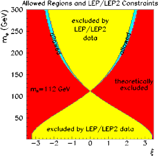
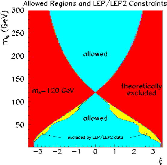
Figure 1: Allowed regions (see text) in $(\xi,m_{\phi})$ parameter space for $\Lambda_{\phi}=5\;\hbox{TeV}$ and $m_{h}=112\;\hbox{GeV}$. The dark red portion of parameter space is theoretically disallowed. The light yellow portion is eliminated by LEP/LEP2 constraints on the $ZZs$ coupling-squared $g_{ZZs}^{2}$ or on $g_{ZZs}^{2}BR(s\to b\overline{b})$, with $s=h$ or $s=\phi$.

Figure 2: As in Fig. 2 but for $m_{h}=120\;\hbox{GeV}$.

The first question that arises is whether both the $\phi$ and the $h$ could be light without either having been detected at LEP and LEP2. The sum rule of Eq. (51) implies that this is impossible since the couplings of the $h$ and $\phi$ to $ZZ$ cannot both be suppressed. For any given value of $m_{h}$ and $m_{\phi}$, the range of $\xi$ is limited by: (a) the constraint of Eq. (37) limiting $\xi$ according to the degree of $m_{h}$–$m_{\phi}$ degeneracy; (b) the constraint that $Z^{2}>0$, Eq. (32); and (c) the requirements that $g_{ZZh}^{2}$ and $g_{ZZ\phi}^{2}$ both lie below any relevant LEP/LEP2 limit. The regions in the $(\xi,m_{\phi})$ plane consistent with the first two constraints as well as $R<5$ are shown in Figs. 2 and 2 for $m_{h}=112\;\hbox{GeV}$ and $m_{h}=120\;\hbox{GeV}$, respectively, assuming a value of $\Lambda_{\phi}=5\;\hbox{TeV}$. For the most part, it is the degeneracy constraint (a) that defines the theoretically acceptable regions shown. The regions within the theoretically acceptable regions that are excluded by the LEP/LEP2 limits are shown by the yellow shaded regions, while the allowed regions are in blue. For $m_{h}=112\;\hbox{GeV}$, the LEP/LEP2 limits exclude a large portion of the theoretically consistent parameter space. For $m_{h}=110\;\hbox{GeV}$ (not plotted), the sum rule of Eq. (51) results in all of the theoretically allowed parameter space being excluded by LEP/LEP2 constraints. For $m_{h}=120\;\hbox{GeV}$, the LEP/LEP2 limits do not apply to the $h$ and it is only for $m_{\phi}\mathrel{\raise 1.29167pt\hbox{$<$\kern-7.5pt\lower 4.30554pt\hbox{$\sim$}}}115\;\hbox{GeV}$ and significant $g_{ZZ\phi}^{2}$ (requiring large $|\xi|$) that some points are ruled out by the LEP/LEP2 constraints. As a result, the allowed region is dramatically larger than for $m_{h}=112\;\hbox{GeV}$. The precise regions shown are somewhat sensitive to the $\Lambda_{\phi}$ choice, but the overall picture is always similar to that presented here for $\Lambda_{\phi}=5\;\hbox{TeV}$. This is illustrated in Sec. 5, where the allowed regions for $m_{h}=120\;\hbox{GeV}$ are shown in the case of $\Lambda_{\phi}=1\;\hbox{TeV}$.

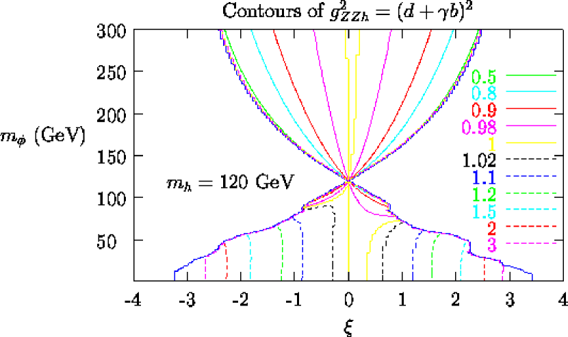
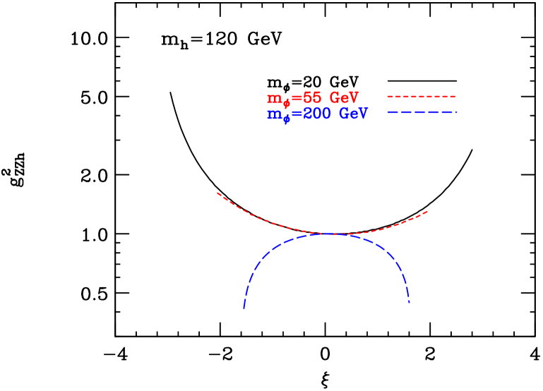
Figure 3: For $m_{h}=120\;\hbox{GeV}$ and $\Lambda_{\phi}=5\;\hbox{TeV}$, we plot the quantity $g_{ZZh}^{2}=(d+\gamma b)^{2}$ which specifies the ratio of the $h$’s $f\overline{f}$ and $VV$ couplings squared to the corresponding values for the SM Higgs boson, taking $m_{h_{SM}}=m_{h}$. In the upper figure we show contours; line colors/textures drawn actually on the boundary should be ignored. The lower figure presents results for $m_{\phi}=20$, $55$ and $200\;\hbox{GeV}$.

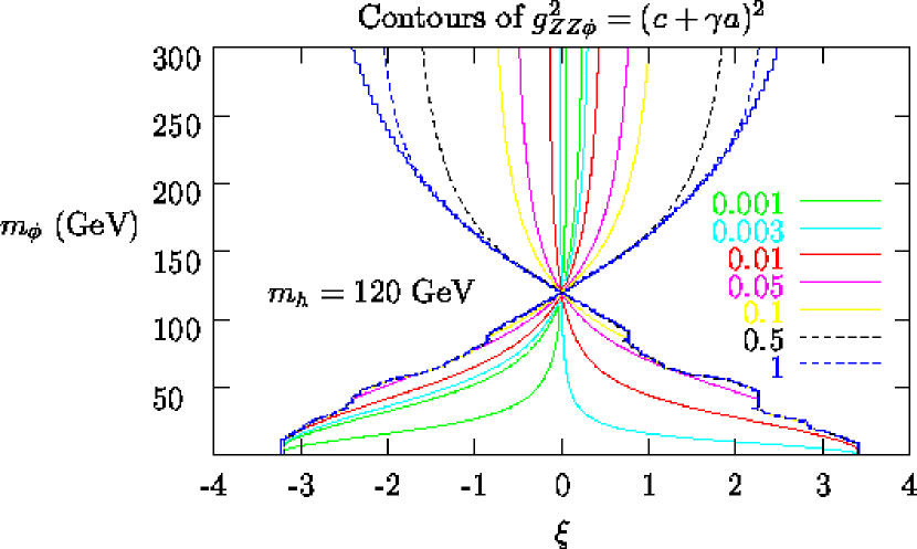
Figure 4: As in Fig. 3, except for the $\phi$. Note the zeroes in the middle of the allowed $\xi$ ranges.

Next, we discuss the couplings of the $h$ and $\phi$. We begin with their $f\overline{f}$ and $VV$ couplings-squared. These are illustrated in Figs. 3 and 4. There we consider $m_{h}=120\;\hbox{GeV}$ and $\Lambda_{\phi}=5\;\hbox{TeV}$ (for which the allowed region was plotted in Fig. 2) and plot (in the upper figures) contours of $g_{ZZh}^{2}\equiv(d+\gamma b)^{2}$ and $g_{ZZ\phi}^{2}\equiv(c+\gamma a)^{2}$. As in Eqs. (47) and (48), these quantities specify the ‘reduced’ couplings squared of the $h$ and $\phi$, respectively, to $f\overline{f}$ and $VV$ with respect to the squared coupling strength of the SM Higgs boson. The lower figures show the variation of these couplings with $\xi$ at fixed $m_{\phi}=20$, $55$ and $200\;\hbox{GeV}$. Large enhancements of $(d+\gamma b)^{2}$ are possible for small $m_{\phi}<m_{h}$ as are large suppressions when $m_{\phi}>m_{h}$. For the $\phi$, $(c+\gamma a)^{2}$ is smaller than 1 except for the largest $|\xi|$ values at high $m_{\phi}$. Indeed, $(c+\gamma a)^{2}\ll 1$ is the norm in the $m_{\phi}<m_{h}$ portion of parameter space and for small $|\xi|$ when $m_{\phi}>m_{h}$. In particular, there is a line along which $(c+\gamma a)^{2}=0$ between the paired contour lines corresponding to $(c+\gamma a)^{2}=0.001$; these zeroes are also apparent from the lower plot of Fig. 4.

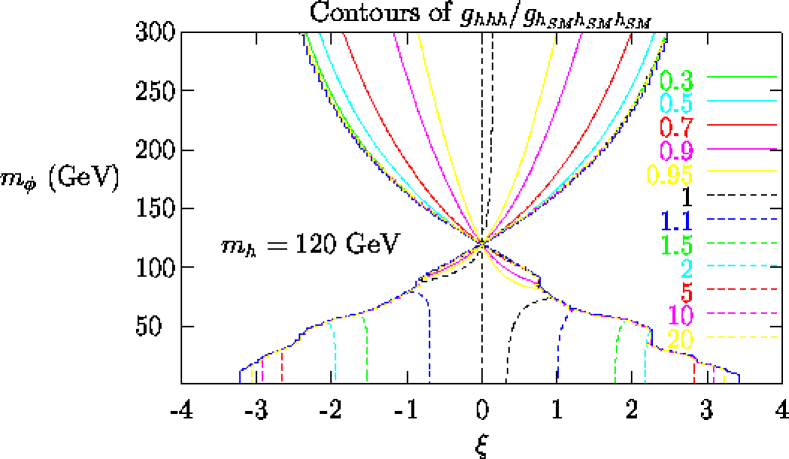
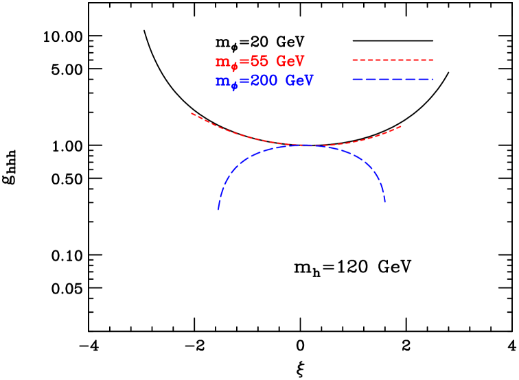
Figure 5: For $m_{h}=120\;\hbox{GeV}$ and $\Lambda_{\phi}=5\;\hbox{TeV}$, we plot the ratio, $g_{hhh}=\overline{g}_{hhh}/\overline{g}_{h_{SM}h_{SM}h_{SM}}$, of the $h^{3}$ self coupling to the SM prediction for the $h_{SM}^{3}$ coupling for $m_{h_{SM}}=m_{h}$. The first plot gives contours, while the 2nd plot shows results at the fixed values of $m_{\phi}=20$, $55$ and $200\;\hbox{GeV}$.

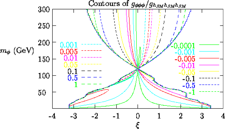
Figure 6: For $m_{h}=120\;\hbox{GeV}$ and $\Lambda_{\phi}=5\;\hbox{TeV}$, we plot the ratio, $g_{\phi\phi\phi}=\overline{g}_{\phi\phi\phi}/\overline{g}_{h_{SM}h_{SM}h_{SM}}$, of the $\phi^{3}$ self coupling to the SM prediction for the $h_{SM}^{3}$ coupling taking $m_{h_{SM}}=m_{\phi}$. The first plot gives contours, while the 2nd plot gives results for $|g_{\phi\phi\phi}|$ at $m_{\phi}=20$, $55$ and $200\;\hbox{GeV}$. In the latter plot, $g_{\phi\phi\phi}$ is: $<0$ for all $\xi$ at $m_{\phi}=20\;\hbox{GeV}$; $>0$ for $\xi<-1.87$ and $<0$ otherwise at $m_{\phi}=55\;\hbox{GeV}$; and $<0$ for $\xi<0.2$ and $>0$ for $\xi>0.2$ at $m_{\phi}=200\;\hbox{GeV}$.

A coupling of particular interest in testing the nature of electroweak symmetry breaking is the $h^{3}$ self coupling. The algebraic form of the $h^{3}$ coupling appears in the Appendix. The SM limit for this coupling corresponds to $d=-a=1$, $c=b=0$. In addition, one employs $\gamma^{-1}/\Lambda_{\phi}=1/v_{0}$. In Fig. 5, we plot the ratio $g_{hhh}\equiv{\overline{g}_{hhh}/\overline{g}_{h_{SM}h_{SM}h_{SM}}}$ of the $h^{3}$ coupling relative to the corresponding SM value computed for a SM Higgs boson mass equal to $m_{h}$. (Recall that, in our notation, a bar indicates the full coupling as opposed to the value relative to the SM, which ratio is indicated by a $g$ without a bar.) We see that there are typically rather substantial deviations that one could easily probe at a linear collider.

It is also interesting to examine the $\phi^{3}$ self coupling. Taking $m_{h_{SM}}=m_{\phi}$, we plot in the upper figure of Fig. 6 contours of $g_{\phi\phi\phi}\equiv\overline{g}_{\phi\phi\phi}/\overline{g}_{h_{SM}h_{SM}h_{SM}}$; in the lower figure, we plot $|g_{\phi\phi\phi}|$. As expected, $g_{\phi\phi\phi}$ vanishes for $\xi=0$. It is often negative (i.e. $\overline{g}_{\phi\phi\phi}$ has the opposite sign compared to $\overline{g}_{h_{SM}h_{SM}h_{SM}}$) and is generally $<1$, implying suppression relative to the SM case. Only for $m_{\phi}=200\;\hbox{GeV}$ and the largest allowed $|\xi|$ values can the $\phi^{3}$ coupling take values comparable to the SM strength. Thus, in general its measurement may be quite difficult. Of course, the ‘background diagrams’ contributing to the same final state ($e^{+}e^{-}\to t\overline{t}\phi\phi$ or $e^{+}e^{-}\to Z\phi\phi$) will also be suppressed in comparison to the SM case; they have two $f\overline{f}\phi$ or $VV\phi$ vertices proportional to $(c+\gamma a)^{2}$, and $(c+\gamma a)^{2}$ is substantially smaller than 1 for much of the parameter space being considered.

A particularly important feature of the above plots is that once $m_{h}$ is large enough ($m_{h}\mathrel{\raise 1.29167pt\hbox{$>$\kern-7.5pt\lower 4.30554pt\hbox{$\sim$}}}115\;\hbox{GeV}$ is sufficient) there is a substantial range of $\xi$ values for any $m_{\phi}<m_{h}/2$ (so that $h\to\phi\phi$ decays are possible) that cannot be excluded by LEP/LEP2 constraints. The reverse is also true; allowed parameter regions exist for which $\phi\to hh$ decays are possible once $m_{\phi}\mathrel{\raise 1.29167pt\hbox{$>$\kern-7.5pt\lower 4.30554pt\hbox{$\sim$}}}230\;\hbox{GeV}$. We now turn to a discussion of branching ratios, including the $h\to\phi\phi$ final mode.

The partial width of the $h$ in which we are most interested is that for $h\to\phi\phi$:

$$\Gamma(h\to\phi\phi)={\overline{g}_{\phi\phi h}^{2}\over 32\pi m_{h}}(1-4r_{\phi})^{1/2}\,.$$ (62)

In the above equation, $\lambda(1,r_{1},r_{2})\equiv 1+r_{1}^{2}+r_{2}^{2}-2r_{1}-2r_{2}-2r_{1}r_{2}$, $r_{\phi}=m_{\phi}^{2}/m_{h}^{2}$. We also give the expression for $h\to h^{n}\phi$:

$$\Gamma(h\to h^{n}\phi)=\frac{\overline{g}_{n\phi h}^{2}}{192\pi}{m_{h}^{3}}{\lambda^{5/2}(1,r_{\phi},r_{n})\over r_{n}^{2}}\,,$$ (63)

where $r_{n}=m_{n}^{2}/m_{h}^{2}$ (Corresponding results apply for $\phi\to hh$ and $\phi\to h^{n}h$.) Expanding in powers of $\gamma=v_{0}/\Lambda_{\phi}$ using Eq. (60), we find that $\Gamma(h\to h^{n}\phi)\sim m_{h}^{3}/r_{n}^{2}\sim m_{h}^{7}$.

It is interesting to investigate Higgs-boson branching ratios for various decay channels in the presence of the $\xi$-mixing. If we neglected the $gg$ and $\gamma\gamma$ anomalous couplings, we would have

$$\Gamma(h\to all)=(d+\gamma b)^{2}\Gamma_{SM}(h\to all)+\Gamma(h\to h^{n}\phi)+\Gamma(h\to\phi\phi)\,,$$ (64)

where $\Gamma_{SM}(h\to all)$ is the SM total width. However, the $gg$ width can be quite enhanced and this must be included. We have done this in the context of a modified version of HDECAY [22], which includes all relevant radiative corrections to couplings and branching ratios. In particular, the running $b$ mass decreases the $b\overline{b}$ branching ratio of the $h$, resulting in some increase in $BR(h\to\phi\phi)$.

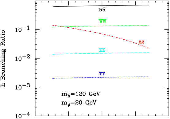
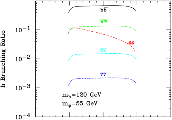
Figure 7: The branching ratios for $h$ decays to $b\overline{b}$, $gg$, $WW^{*}$, $ZZ^{*}$ and $\gamma\gamma$ for $m_{h}=120\;\hbox{GeV}$ and $\Lambda_{\phi}=5\;\hbox{TeV}$ as functions of $\xi$ for $m_{\phi}=20$, $55$ and $200\;\hbox{GeV}$.

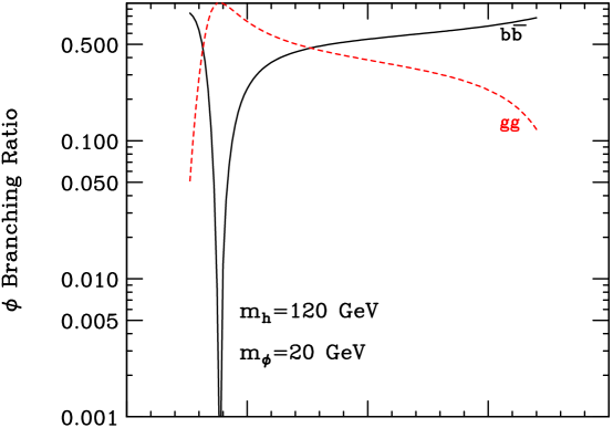
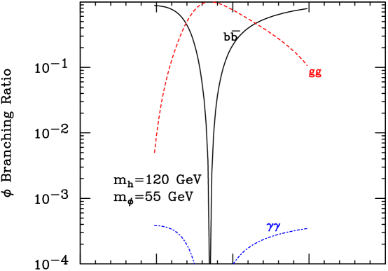
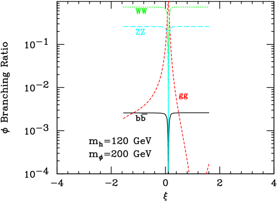
Figure 8: The branching ratios for $\phi$ decays to $b\overline{b}$, $gg$, $WW^{(*)}$, $ZZ^{(*)}$ and $\gamma\gamma$ for $m_{h}=120\;\hbox{GeV}$ and $\Lambda_{\phi}=5\;\hbox{TeV}$ as functions of $\xi$ for $m_{\phi}=20$, $55$ and $200\;\hbox{GeV}$.

In Fig. 7, we plot the branching ratios for $h\to b\overline{b}$, $gg$, $WW^{*}$, $ZZ^{*}$ and $\gamma\gamma$ as a function of the mixing parameter $\xi$, taking $m_{h}=120\;\hbox{GeV}$ and $\Lambda_{\phi}=5\;\hbox{TeV}$. Results are shown for three different $m_{\phi}$ values: $20$, $55$ and $200\;\hbox{GeV}$. (The case of $m_{\phi}=55\;\hbox{GeV}$ is one for which $BR(h\to\phi\phi)$ can be quite large when $m_{h}=120\;\hbox{GeV}$.) These plots are limited to $\xi$ values allowed by the theoretical constraints discussed earlier. We have chosen to not include a more restrictive bound on $g_{ZZh}^{2}$ as might be appropriate in order to guarantee that the $h$ contributions to precision electroweak observables be consistent with $S$ and $T$ remaining within the usual $95\%$ CL ellipse. Fig. 3 shows that $g_{ZZh}^{2}>2$ (a rough estimate of the needed bound) only at the very largest $|\xi|$ values when $m_{\phi}$ is small.

The most important features of Fig. 7 are the following. First, large values for the $gg$ branching ratio (due to the anomalous contribution to the $hgg$ coupling) are the norm. This suppresses the other branching ratios to some extent. (The anomalous contribution to the $h\gamma\gamma$ coupling is less important due to presence of the large $W$ loop contribution in this latter case.) Second, for $m_{\phi}=55\;\hbox{GeV}$, $BR(h\to\phi\phi)$ is large at large $|\xi|$ and suppresses the conventional branching ratios. In general, changes in the branching ratio of the $h$ with respect to the SM are modest, but nonetheless they are at an observable level, at least at the LC. Note, however, that the modest $BR$ changes belie the fact that the $f\overline{f}$ and $VV$ coupling-squared factor $(c+\gamma d)^{2}$ is often changing dramatically, implying dramatic changes in $h$ production rates with respect to expectations for a SM $h_{SM}$.

Results for the $\phi$ branching ratios are plotted in Fig. 8. We observe that the $gg$ decay is generally dominant over the $b\overline{b}$ mode and that it has the largest branching ratio until the $WW^{(*)},ZZ^{(*)}$ modes increase in importance at larger $m_{\phi}$. Of course, the zero in $g_{ZZ\phi}^{2}=(c+\gamma a)^{2}$ has a very large impact.

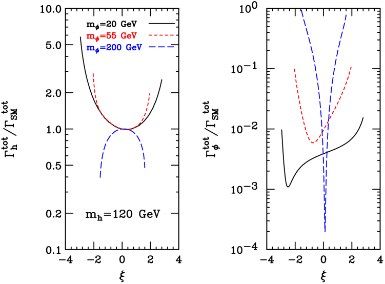
Figure 9: The total widths for the $h$ and $\phi$ relative to the value for a SM Higgs boson of the same mass are plotted as functions of $\xi$ for $m_{h}=120\;\hbox{GeV}$ and $\Lambda_{\phi}=5\;\hbox{TeV}$ taking $m_{\phi}=20$, $55$ and $200\;\hbox{GeV}$.

Also important for $h$ discovery is its total width. In the left-hand window of Fig. 9, we plot the ratio of the total $h$ width to the corresponding width of a SM Higgs boson of the same mass, $\Gamma_{h}^{\rm tot}/\Gamma_{SM}^{\rm tot}$, as a function of $\xi$ for $m_{\phi}=20$, $55$ and $200\;\hbox{GeV}$. Note that a substantially larger total width for the $h$ is possible if $m_{\phi}$ is small. In the right-hand window, we plot the ratio $\Gamma_{\phi}^{\rm tot}/\Gamma_{SM}^{\rm tot}$ (for $m_{h_{SM}}=m_{\phi}$) as a function of $\xi$. The $\phi$ is generally quite narrow. This is true even for $m_{\phi}=200\;\hbox{GeV}$, for which $WW/ZZ$ decays are allowed, near the zero in $(c+\gamma a)^{2}$.

Figure 10: The ratio of the rates for $gg\to h\to\gamma\gamma$ and $WW\to h\to\tau^{+}\tau^{-}$ (the latter is the same as that for $gg\to t\overline{t}h\to t\overline{t}b\overline{b}$) to the corresponding rates for the SM Higgs boson. Results are shown for $m_{h}=120\;\hbox{GeV}$ and $\Lambda_{\phi}=5\;\hbox{TeV}$ as functions of $\xi$ for $m_{\phi}=20$, $55$ and $200\;\hbox{GeV}$.

Experimentally, the above results imply that detection of the $h$ at the LHC could be significantly impacted if $|\xi|$ is large. To illustrate this, we plot in Fig. 10 the ratio of the rates for $gg\to h\to\gamma\gamma$, $WW\to h\to\tau^{+}\tau^{-}$ and $gg\to t\overline{t}h\to t\overline{t}b\overline{b}$ (the latter two ratios being equal) to the corresponding rates for the SM Higgs boson. For this figure, we take $m_{h}=120\;\hbox{GeV}$ and $\Lambda_{\phi}=5\;\hbox{TeV}$ and show results for $m_{\phi}=20$, $55$ and $200\;\hbox{GeV}$. In the case of $m_{\phi}=55\;\hbox{GeV}$, the $h\to\phi\phi$ decay, discussed in more detail later, is substantial for large $|\xi|$. The resulting suppression of the standard LHC modes at the largest allowed $|\xi|$ values is most evident in the $W^{+}W^{-}\to h\to\tau^{+}\tau^{-}$ curves. Another important impact of mixing is through communication of the anomalous $gg$ coupling of the $\phi_{0}$ to the $h$ mass eigenstate. The result is that prospects for $h$ discovery in the $gg\to h\to\gamma\gamma$ mode could be either substantially poorer or substantially better than for a SM Higgs boson of the same mass, depending on $\xi$ and $m_{\phi}$.

At the LC, the potential for $h$ discovery is primarily determined by $g_{ZZh}^{2}$. As shown in Fig. 3, this reduced coupling-squared (defined relative to the SM value) is often $>1$ (and can be as large as $\sim 5$), but can also fall to values as low as $\sim 0.4$, implying signficant suppression relative to SM expectations. The latter suppression is well within the reach of the $e^{+}e^{-}\to Zh$ recoil mass discovery technique at a LC with $\sqrt{s}=500\;\hbox{GeV}$ and $L=500~{}\mbox{fb${}^{-1}$}$. The techniques that have been developed for measuring the total width of a Higgs boson at the LC indirectly would remain applicable and could reveal the presence of $\xi\neq 0$ mixing through a sizable deviation with respect to the SM prediction.

Figure 11: The ratio of the rates for $gg\to\phi\to\gamma\gamma$ and for $WW\to\phi\to\tau^{+}\tau^{-}$ (the latter being the same as that for $gg\to t\overline{t}\phi\to t\overline{t}b\overline{b}$) to the corresponding rates for the SM Higgs boson. Results are shown for $m_{h}=120\;\hbox{GeV}$ and $\Lambda_{\phi}=5\;\hbox{TeV}$ as functions of $\xi$ for $m_{\phi}=20$, $55$ and $200\;\hbox{GeV}$.

Figure 12: As in Fig. 11, but for $m_{\phi}=110$ and $140\;\hbox{GeV}$.

Figure 13: The ratio of the rate for $gg\to\phi\to ZZ$ to the corresponding rate for a SM Higgs boson with mass $m_{\phi}$ assuming $m_{h}=120\;\hbox{GeV}$ and $\Lambda_{\phi}=5\;\hbox{TeV}$ as a function of $\xi$ for $m_{\phi}=110$, $140$ and $200\;\hbox{GeV}$. Recall that the $\xi$ range is increasingly restricted as $m_{\phi}$ becomes more degenerate with $m_{h}$.

What about prospects for $\phi$ detection at the LHC? In Figs. 11 and 12, we plot the same ratios for the $\phi$ as we did for the $h$ in Fig. 10. For this figure, we take $m_{h}=120\;\hbox{GeV}$ and $\Lambda_{\phi}=5\;\hbox{TeV}$ and show results for $m_{\phi}=20$, $55$ and $200\;\hbox{GeV}$ in Fig. 11 and for $m_{\phi}=110$ and $140\;\hbox{GeV}$ in Fig. 12. For all masses, the $gg\to\phi\to\gamma\gamma$ rate is generally significantly suppressed relative to the prediction for a SM Higgs boson, depending upon $\xi$ and $m_{\phi}$. The dip in the $\phi$ rates is due to a cancellation that zeroes the $\gamma\gamma$ coupling, and occurs very close to the point at which the $\phi$’s couplings to vector bosons and fermions, $(c+\gamma a)^{2}$, vanishes. Detection of the $\phi$ in $gg\to\phi\to\gamma\gamma$ will generally be quite difficult. The $WW\to\phi\to\tau^{+}\tau^{-}$ and $gg\to t\overline{t}\phi\to t\overline{t}b\overline{b}$ modes are generally also quite suppressed relative to SM rates and would probably not be visible. For $m_{\phi}\mathrel{\raise 1.29167pt\hbox{$>$\kern-7.5pt\lower 4.30554pt\hbox{$\sim$}}}110\;\hbox{GeV}$, in addition to the above three modes one can consider the standard $gg\to\phi\to ZZ^{(*)}\to 4\ell$ signal. The ratio for this rate relative to the SM prediction is plotted in Fig. 13 for $m_{\phi}=110$, $140$ and $200\;\hbox{GeV}$. For $m_{\phi}=200\;\hbox{GeV}$, the very high level of statistical significance predicted for the SM $ZZ$ final state signal at this mass implies that $\phi$ detection in this mode should be possible except near the zeroes in the $ZZ\phi$ coupling. For the $m_{\phi}=110$ and $140\;\hbox{GeV}$ cases, the dip region occupies a lot of the allowed $\xi$ range and suppression is generally present even away from the dip regions. Detection in the $4\ell$ mode would be unlikely.

At the LC, the potential for $\phi$ discovery is primarily determined by $g_{ZZ\phi}^{2}$. As shown in Fig. 4, this reduced coupling-squared is typically substantially suppressed relative to the SM value of 1. Still, because of the very high statistical significance associated with a SM Higgs signal in the $e^{+}e^{-}\to Z$+Higgs mode for $\sqrt{s}=500\;\hbox{GeV}$ and $L=500~{}\mbox{fb${}^{-1}$}$, detection of the $\phi$ will be possible except near the zero in the $ZZ\phi$ coupling. As discussed earlier, the width of the $\phi$ would be much smaller than anticipated. This could be checked using the techniques that have been developed for measuring the total width of a narrow Higgs boson at the LC indirectly.

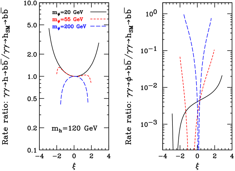
Figure 14: The rates for $\gamma\gamma\to h\to b\overline{b}$ and $\gamma\gamma\to\phi\to b\overline{b}$ relative to the corresponding rate for a SM Higgs boson of the same mass. Results are shown for $m_{h}=120\;\hbox{GeV}$ and $\Lambda_{\phi}=5\;\hbox{TeV}$ as functions of $\xi$ for $m_{\phi}=20$, $55$ and $200\;\hbox{GeV}$.

Also of considerable interest is how $\xi\neq 0$ would affect prospects for $h$ and $\phi$ detection at a $\gamma\gamma$ collider. To assess this, we plot in Fig. 14 the $\gamma\gamma\to h\to b\overline{b}$ and $\gamma\gamma\to\phi\to b\overline{b}$ rates relative to the SM rates evaluated for Higgs mass equal to $m_{h}$ or $m_{\phi}$, respectively. In the case of the $h$, the plot differs only slightly from Fig. 10 for the $WW\to h\to\tau^{+}\tau^{-}$ LHC discovery mode. This means that the anomaly contribution to the $\gamma\gamma h$ coupling is much smaller than that from the standard fermion and $W$ boson loops. In the case of the $\phi$, differences between these $\gamma\gamma\to\phi\to b\overline{b}$ curves and the corresponding $WW\to\phi\to\tau^{+}\tau^{-}$ curves of Fig. 11 are somewhat larger, especially in the vicinity of the zeroes.

To summarize the results, in the case of the $h$, for the parameters considered, the rate is suppressed by at most a factor of 0.5 and would thus be quite sufficient to yield a highly detectable and accurately measurable signal. The $\phi$ would typically be much more difficult to discover in $\gamma\gamma$ collisions. Large dips in the rate occur in the vicinity of the zero in the $\phi\to b\overline{b}$ coupling and branching ratio, which is at the same location as the zero in $g_{ZZ\phi}$. The $\gamma\gamma\to\phi\to gg$ channel is somewhat less suppressed in the dip region due to the anomalous contribution to the $\phi gg$ coupling. However, the signal is still small in the dip regions and this channel would have large backgrounds. Although it would be difficult to isolate, further study might be warranted.

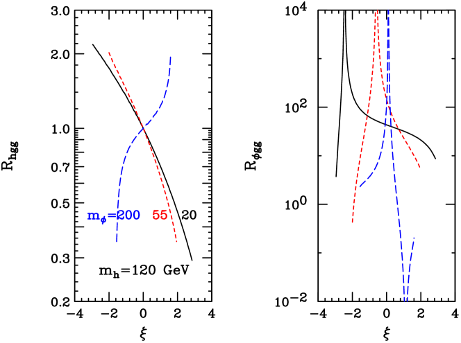
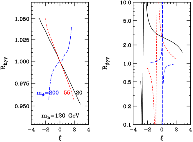
Figure 15: In the upper plots, we give the ratios $R_{hgg}$ and $R_{\phi gg}$ of the $hgg$ and $\phi gg$ couplings-squared including the anomalous contribution to the corresponding values expected in its absence. Results for the the analogous ratios $R_{h\gamma\gamma}$ and $R_{\phi\gamma\gamma}$ are presented in the lower plots. Results are shown for $m_{h}=120\;\hbox{GeV}$ and $\Lambda_{\phi}=5\;\hbox{TeV}$ as functions of $\xi$ for $m_{\phi}=20$, $55$ and $200\;\hbox{GeV}$. (The same type of line is used for a given $m_{\phi}$ in the right-hand figure as is used in the left-hand figure.)

An important question is whether the deviations due to the anomalous $\phi_{0}gg$ and $\phi_{0}\gamma\gamma$ couplings are sufficiently large to be measurable. To quantify this, we plot in Fig. 15 the ratios 

$$R_{sgg}\equiv{\overline{g}_{sgg}^{2}(\mbox{with anomaly})\over\overline{g}_{sgg}^{2}(\mbox{without anomaly})}\,,\quad\mbox{and}\quad R_{s\gamma\gamma}\equiv{\overline{g}_{s\gamma\gamma}^{2}(\mbox{with anomaly})\over\overline{g}_{s\gamma\gamma}^{2}(\mbox{without anomaly})}\,,$$ (65)

for $s=h$ and $s=\phi$. These ratios can be determined experimentally. First, (model-independent) measurements of the $g_{ZZh}^{2}=(d+\gamma b)^{2}$ and $g_{ZZ\phi}^{2}=(c+\gamma a)^{2}$ coupling factors for the $h$ and $\phi$ are obtained using $e^{+}e^{-}\to Zh$ and $e^{+}e^{-}\to Z\phi$ production at the linear collider. The $sgg$ and $s\gamma\gamma$ couplings ($s=h$ or $\phi$) expected from the standard fermion and $W$-boson loops in the absence of the anomalous contribution can then be computed. Meanwhile, the actual couplings-squared, $\overline{g}_{sgg}^{2}$ and $\overline{g}_{s\gamma\gamma}^{2}$, including any anomalous contribution, can be directly measured using a combination of $\gamma\gamma\to s\to b\overline{b}$ and $gg\to s\to\gamma\gamma$ data.

In more detail, we employ the following procedures.

• First, obtain $g_{ZZs}^{2}$ (defined relative to the SM prediction at $m_{h_{SM}}=m_{s}$) from $\sigma(e^{+}e^{-}\to Zs)$ (inclusive recoil technique).

• Next, determine $BR(s\to b\overline{b})=\sigma(e^{+}e^{-}\to Zs\to Zb\overline{b})/\sigma(e^{+}e^{-}\to Zs)$.

• Then, compute $\overline{g}_{s\gamma\gamma}^{2}$ from $\sigma(\gamma\gamma\to s\to b\overline{b})/BR(s\to b\overline{b})$.

• To display the contribution to the $s\gamma\gamma$ coupling-squared from the anomaly one would then compute

  $$R_{s\gamma\gamma}\equiv{\overline{g}_{s\gamma\gamma}^{2}(\mbox{from experiment})\over\overline{g}_{h_{SM}\gamma\gamma}^{2}(\mbox{as computed for $m_{h_{SM}}=m_{s}$})\times g_{ZZs}^{2}(\mbox{from experiment})}$$ (66)

• To determine $\overline{g}_{sgg}^{2}$ experimentally requires one more step. We must compute $\sigma(gg\to s\to\gamma\gamma)/BR(s\to\gamma\gamma)$. To obtain $BR(s\to\gamma\gamma)$, we need a measurement of $\Gamma_{s}^{\rm tot}$.

  Given such a measurement, we then compute

  $$BR(s\to\gamma\gamma)={\Gamma(s\to\gamma\gamma)(\mbox{computed from $\overline{g}_{s\gamma\gamma}^{2}$})\over\Gamma_{s}^{\rm tot}(\mbox{from experiment})}\,,$$ (67)

  where the above experimental determination of $\overline{g}_{s\gamma\gamma}^{2}$ is employed and the experimental techniques outlined in [23] are employed for $\Gamma_{s}^{\rm tot}$.

• The ratio analogous to Eq. (66) for the $gg$ coupling is then

  $$R_{sgg}\equiv{\overline{g}_{sgg}^{2}(\mbox{from experiment})\over\overline{g}_{h_{SM}gg}^{2}(\mbox{as computed for $m_{h_{SM}}=m_{s}$})\times g_{ZZs}^{2}(\mbox{from experiment})}\,.$$ (68)

For a light SM Higgs boson, the various cross sections and branching ratios needed for the $s\gamma\gamma$ coupling can be determined with errors of order a few percent [23]. We see from Fig. 15 that for large $\xi$ this level of accuracy is on the edge of being sufficient to detect the deviation in the case of the $h$. In the case of the $\phi$, the expected deviation is typically much larger, especially near the zeroes in the rates. Indeed, the size of the deviation is largest when the $\phi$ rate is smallest. A careful study is needed to assess the prospects. For the $gg$ coupling, errors might be dominated by the accuracy with which the total width can be determined. Estimates for this error in the case of the SM $h_{SM}$ are in the neighborhood of $10\%$ for $m_{h_{SM}}=120\;\hbox{GeV}$ [23], decreasing for higher $m_{h_{SM}}$. Thus, the factor of two deviations expected in the case of the $hgg$ coupling-squared at the higher $\xi$ values might well be discernable experimentally. Since the $\phi$ may prove difficult to detect at the LHC, a much more detailed study is required to see if deviations in the $\phi gg$ coupling due to the anomalous contribution could be detected.

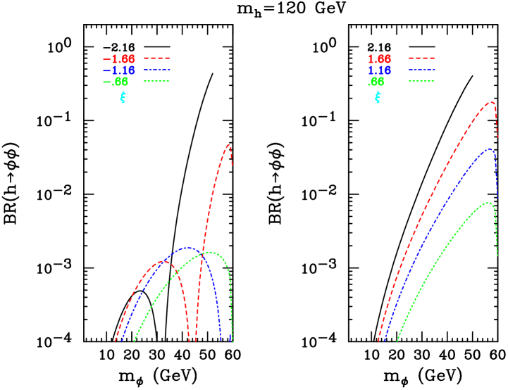
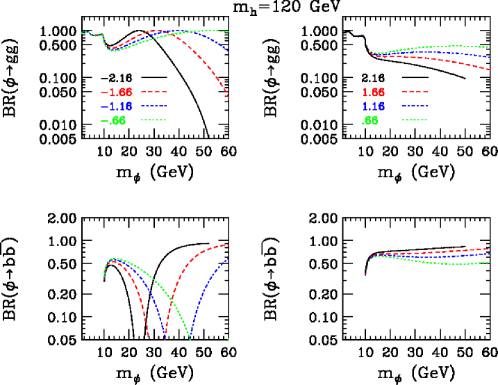
Figure 16: The branching ratios for $h\to\phi\phi$, $\phi\to gg$ and $\phi\to b\overline{b}$ for $m_{h}=120\;\hbox{GeV}$ and $\Lambda_{\phi}=5\;\hbox{TeV}$ as a function of $m_{\phi}$ for $\xi=-2.16$, $-1.66$, $-1.16$ and $-0.66$ (left-hand graphs) and for $\xi=0.66$, $1.16$, $1.66$, and $2.16$ (right-hand graphs).

We will now turn to a more thorough exploration of the parameter regions in which $h\to\phi\phi$ decays are large. The branching ratios for $h\to\phi\phi$ in the case of $m_{h}=120\;\hbox{GeV}$ and $\Lambda_{\phi}=5\;\hbox{TeV}$ are shown in Fig. 16 for various $\xi$ choices within the allowed region. The plots show that $h\to\phi\phi$ decays can be quite important at the largest $|\xi|$ values when $m_{\phi}$ is close to $m_{h}/2$. Detection of the $h\to\phi\phi$ decay mode could easily provide the most striking evidence for the presence of $\xi\neq 0$ mixing. In order to understand how to search for the $h\to\phi\phi$ decay mode, it is useful to know how the $\phi$ decays. In Fig. 16 we give detailed results for $BR(\phi\to gg)$ and $BR(\phi\to b\overline{b})$ for the same $m_{\phi}$ and $\xi$ values for which $BR(h\to\phi\phi)$ is plotted. (The $c\overline{c}$ and $\tau^{+}\tau^{-}$ channels supply the remainder.) For $\xi>0$, $BR(\phi\to b\overline{b})$ is always substantial and might make detection of the $h\to\phi\phi\to 4b$ and $h\to\phi\phi\to 2g2b$ final states possible. The $\phi\to\gamma\gamma$ decay mode always has a very tiny branching ratio and the related detection channels would not be useful.

One will probably first search for the $h$ in the modes that have been shown to be viable for the SM Higgs boson. We have given in Fig. 10 the rates for important LHC discovery modes relative to the corresponding SM values in the case of $m_{\phi}=55\;\hbox{GeV}$. Results for other $m_{\phi}<m_{h}/2$ values are similar in nature. We observe that the $WW\to h\to\tau^{+}\tau^{-}$ and $gg\to t\overline{t}h\to t\overline{t}b\overline{b}$ detection modes are generally sufficiently mildly suppressed that detection of the $h$ in these modes should be possible (assuming full $L=300~{}\mbox{fb${}^{-1}$}$ luminosity per detector). The $gg\to h\to\gamma\gamma$ detection mode could either be enhanced or significantly suppressed relative to the SM expectation. Once the $h$ has been detected in one of the SM modes, a dedicated search for the $h\to\phi\phi\to b\overline{b}b\overline{b}$ and $h\to\phi\phi\to b\overline{b}gg$ decay modes will be important. At the LHC, backgrounds for these modes will be substantial and a thorough Monte Carlo assessment is needed.

At the LC, since $g_{ZZh}^{2}$ is close to 1 (relative to the SM Higgs value), the $h$ will be readily detectable using the recoil mass procedure in $e^{+}e^{-}\to Zh$ events. Once the $h$ mass peak is detected, it should be possible to delineate in detail the $h$ and $\phi$ branching ratios.

As for detection of the $\phi$ at the LC, the most relevant quantity is $g_{ZZ\phi}^{2}$. Detailed plots of this quantity appear in Fig. 4. These plots indicate that LC detection of $e^{+}e^{-}\to Z\phi$ using the recoil mass method will require being far from the zero in $g_{ZZ\phi}^{2}$. For a significant portion of parameter space, it seems quite apparent that the only way to detect the $\phi$ would be through the $h\to\phi\phi$ decays.

In order to have substantial $BR(h\to\phi\phi)$ it is necessary that $m_{h}<2m_{W}$. As $m_{h}$ is increased above $2m_{W}$, the $WW$ and then $ZZ$ modes become strong and overwhelm the $\phi\phi$ decay mode. For example, for $m_{h}=200\;\hbox{GeV}$, the largest value found for $BR(h\to\phi\phi)$ is of order $1\div 2\,\%$, and such values are again achieved when $|\xi|$ is as large as possible and $m_{\phi}$ is just below $m_{h}/2$.

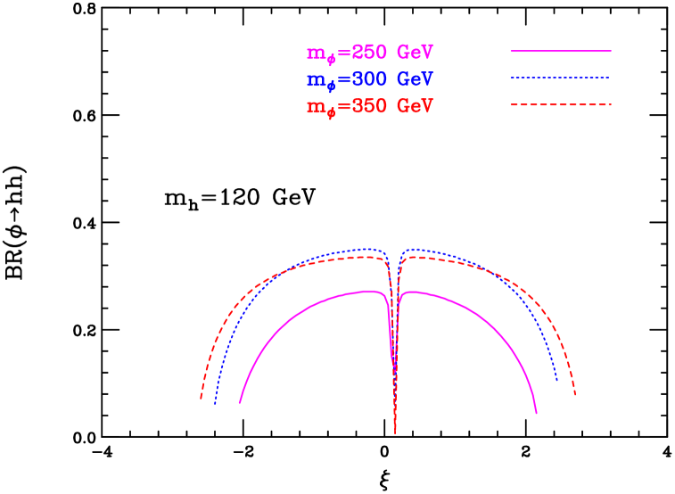
Figure 17: The $\phi\to hh$ branching ratio is plotted as a function of $\xi$ for $m_{h}=120\;\hbox{GeV}$ and $m_{\phi}=250$, $300$ and $350\;\hbox{GeV}$. We have taken $\Lambda_{\phi}=5\;\hbox{TeV}$ and assumed $m_{1}>m_{\phi}$.

Let us now discuss $\phi\to hh$ decays. For $m_{h}=120\;\hbox{GeV}$, these are present once $m_{\phi}\mathrel{\raise 1.29167pt\hbox{$>$\kern-7.5pt\lower 4.30554pt\hbox{$\sim$}}}240\;\hbox{GeV}$. When allowed, these decays will be quite strong since the $\phi hh$ coupling is typically larger than the $h\phi\phi$ coupling away from zeroes in the coupling. In addition, the $\phi$ decays to $f\overline{f}$ and $VV$ are typically suppressed compared to those of the $h$ because of the smaller size of $(c+\gamma a)^{2}$ compared to $(d+\gamma b)^{2}$ when $m_{\phi}>m_{h}$ (see Figs. 3 and 4) for all but the largest $|\xi|$ values. The importance of the $\phi\to hh$ decays is illustrated for $m_{h}=120\;\hbox{GeV}$ and $m_{\phi}=250$ $300$ and $350\;\hbox{GeV}$ in Fig. 17. Even though $m_{\phi}>2m_{W}$ in all these cases, $BR(\phi\to hh)$ is still of order $0.3\div 0.4$ for most of the allowed $\xi$ range not near a zero in the $\phi hh$ coupling.

5 Phenomenology for $\Lambda_{\phi}=1\;\hbox{TeV}$

In this section, we consider the more marginal choice of $\Lambda_{\phi}=1\;\hbox{TeV}$. For this case, we will consider first results obtained assuming $m_{1}$ is large ($>1\;\hbox{TeV}$). As discussed earlier, such large $m_{1}$ requires large curvature, $m_{0}/M_{Pl}\sim\mathcal{O}(1)$, that would presumably imply significant corrections to the RS ansatz. Nonetheless, the large-$m_{1}$ results provide a useful benchmark that might provide a reasonable first approximation in such a case. We also noted that for $\Lambda_{\phi}=1\;\hbox{TeV}$ and $m_{0}/M_{Pl}\sim 1$ large $m_{1}$ is needed to clearly avoid any constraints from RunI Tevatron data. We next consider results obtained in two small-curvature cases: $m_{0}/M_{Pl}\sim 0.065$ and $\sim 0.195$, corresponding to $m_{1}=100$ and $300\;\hbox{GeV}$, respectively. As discussed, such small $m_{1}$ values might or might not be inconsistent with constraints from current RunI Tevatron data and from the $S$ and $T$ electroweak observables. However, the very interesting physics associated with Higgs decays to KK excitations that emerges deserves attention just in case this scenario should arise. In our presentation for $\Lambda_{\phi}=1\;\hbox{TeV}$, we focus only on the significant changes as compared to $\Lambda_{\phi}=5\;\hbox{TeV}$.

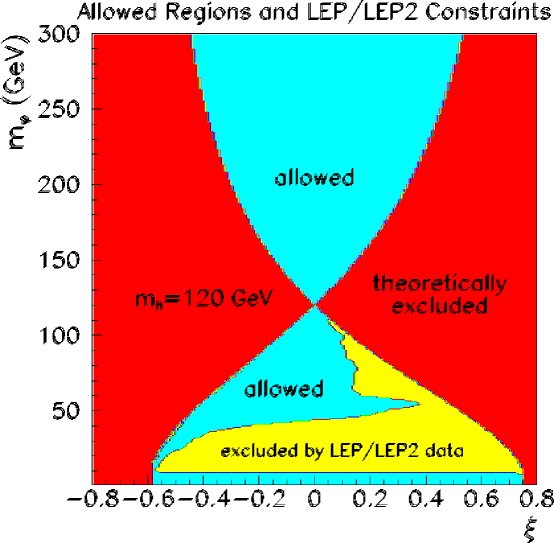
Figure 18: As in Fig. 2 but for $\Lambda_{\phi}=1\;\hbox{TeV}$. The region of theoretically allowed $\xi>0$ values below $\sim 0.45$ with $55\;\hbox{GeV}\mathrel{\raise 1.29167pt\hbox{$<$\kern-7.5pt\lower 4.30554pt\hbox{$\sim$}}}m_{\phi}\mathrel{\raise 1.29167pt\hbox{$<$\kern-7.5pt\lower 4.30554pt\hbox{$\sim$}}}115\;\hbox{GeV}$ that are in the yellow LEP/LEP2-excluded region will be referred to as the ‘LE’ region.

Figure 19: For $m_{h}=120\;\hbox{GeV}$ and $\Lambda_{\phi}=1\;\hbox{TeV}$, we plot contours for $g_{ZZ\phi}^{2}=(c+\gamma a)^{2}$ inside the region that can only be excluded if we assume the limits of [18] apply. The two thick (magenta) lines are the $\xi$ values such that $g_{ZZh}^{2}=2$. The region between these lines has $g_{ZZh}^{2}<2$ and is that most likely to be consistent with precision electroweak data.

First, we present the allowed region in $(\xi,m_{\phi})$ parameter space for $m_{h}=120\;\hbox{GeV}$ in Fig. 18. Of course, the allowed $\xi$ range is very much reduced compared to $\Lambda_{\phi}=5\;\hbox{TeV}$ since $\gamma$ is five times larger; see Eq. (52). As compared to Fig. 2, we see that there is a significant region with lower $m_{\phi}$, but with $m_{\phi}\mathrel{\raise 1.29167pt\hbox{$>$\kern-7.5pt\lower 4.30554pt\hbox{$\sim$}}}8\;\hbox{GeV}$, that is excluded by the LEP/LEP2 limits coming from untagged hadronic events and/or from $b$-tagged final states. A similar region is not excluded in the $\Lambda_{\phi}=5\;\hbox{TeV}$ case because the $g_{ZZ\phi}^{2}$ coupling for $\Lambda_{\phi}=5\;\hbox{TeV}$ is substantially smaller than for $\Lambda_{\phi}=1\;\hbox{TeV}$. Returning to the $\Lambda_{\phi}=1\;\hbox{TeV}$ case, points with $m_{\phi}\mathrel{\raise 1.29167pt\hbox{$<$\kern-7.5pt\lower 4.30554pt\hbox{$\sim$}}}8\;\hbox{GeV}$ are not exluded because the upper bound on $g_{ZZ\phi}^{2}$ coming from untagged hadronic final states rises very rapidly as one moves to lower masses and there are no limits from $b$-tagged final states. However, we should note that if the limits of [18] apply (we have assumed they do not because of the dominance of $\phi\to gg$ decays), for $\Lambda_{\phi}=1\;\hbox{TeV}$ the $m_{\phi}\mathrel{\raise 1.29167pt\hbox{$<$\kern-7.5pt\lower 4.30554pt\hbox{$\sim$}}}8\;\hbox{GeV}$ region would be excluded as well as the $m_{\phi}\mathrel{\raise 1.29167pt\hbox{$>$\kern-7.5pt\lower 4.30554pt\hbox{$\sim$}}}8\;\hbox{GeV}$ regions shown. As illustrated in Fig. 19, for $\Lambda_{\phi}=1\;\hbox{TeV}$ the magnitude of $g_{ZZ\phi}^{2}$ in this low-$m_{\phi}$ region is not so very small.

In what follows, it will be convenient to include in some of our plots some $(\xi,m_{\phi})$ values that are marked as LEP/LEP2-excluded in Fig. 18: namely, we include all those theoretically allowed $\xi>0$ values below $\sim 0.45$ with $55\;\hbox{GeV}\mathrel{\raise 1.29167pt\hbox{$<$\kern-7.5pt\lower 4.30554pt\hbox{$\sim$}}}m_{\phi}\mathrel{\raise 1.29167pt\hbox{$<$\kern-7.5pt\lower 4.30554pt\hbox{$\sim$}}}115\;\hbox{GeV}$ that are marked in yellow. We will refer to this region as region ‘LE’ in what follows.

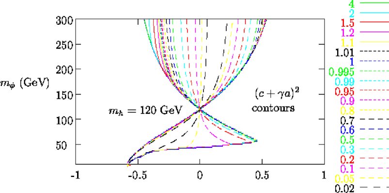
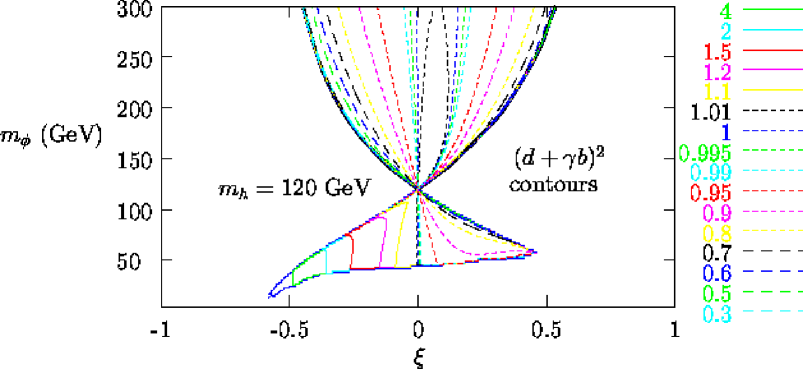
Figure 20: For $m_{h}=120\;\hbox{GeV}$ and $\Lambda_{\phi}=1\;\hbox{TeV}$, we plot contours for the quantities $(d+\gamma b)^{2}$ and $(c+\gamma a)^{2}$. For $(d+\gamma b)^{2}$, only the region $m_{\phi}\geq 15\;\hbox{GeV}$ is shown. For $(c+\gamma a)^{2}$, we show the narrow pipe that connects to the allowed region of very small $m_{\phi}$; see Fig. 19.

Contours of $g_{ZZh}^{2}=(d+\gamma b)^{2}$ and $g_{ZZ\phi}^{2}=(c+\gamma a)^{2}$ are presented in Fig. 20. There, we see that region LE is excluded by LEP/LEP2 data because in this region the $g_{ZZ\phi}^{2}$ value gets to be a reasonable fraction of one, the SM value. Globally speaking, the main difference between the couplings for $\Lambda_{\phi}=1\;\hbox{TeV}$ versus those for $\Lambda_{\phi}=5\;\hbox{TeV}$ of Figs. 3 and 4 is that $g_{ZZ\phi}^{2}$ is overall much larger in the $\Lambda_{\phi}=1\;\hbox{TeV}$ case.

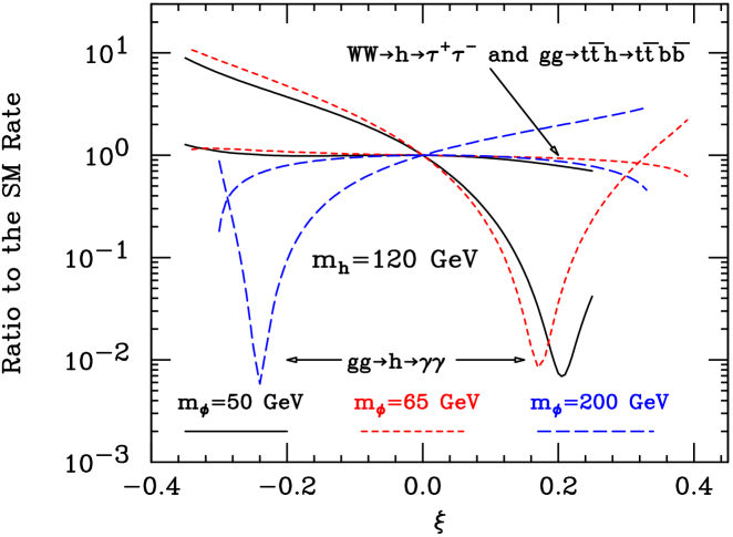
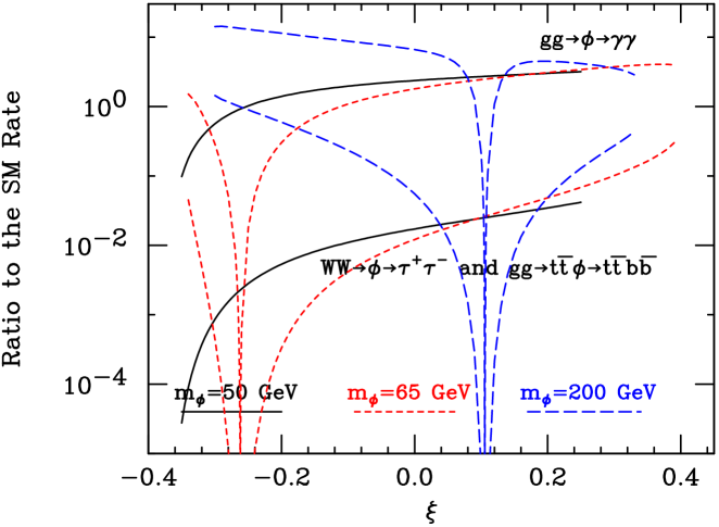
Figure 21: The ratio of the rates for $gg\to h\to\gamma\gamma$ and $WW\to h\to\tau^{+}\tau^{-}$ (the latter being the same as that for $gg\to t\overline{t}h\to t\overline{t}b\overline{b}$) to the corresponding rates for the SM Higgs boson. Results are shown for $m_{h}=120\;\hbox{GeV}$ and $\Lambda_{\phi}=1\;\hbox{TeV}$ as functions of $\xi$ for $m_{\phi}=50$, $65$ and $200\;\hbox{GeV}$.

Figure 22: The ratio of the rates for $gg\to\phi\to\gamma\gamma$ (the higher curves for a given $m_{\phi}$) and for $WW\to\phi\to\tau^{+}\tau^{-}$ (the latter being the same as that for $gg\to t\overline{t}\phi\to t\overline{t}b\overline{b}$) to the corresponding rates for the SM Higgs boson. Results are shown for $m_{h}=120\;\hbox{GeV}$ and $\Lambda_{\phi}=1\;\hbox{TeV}$ as functions of $\xi$ for $m_{\phi}=50$, $65$ and $200\;\hbox{GeV}$.

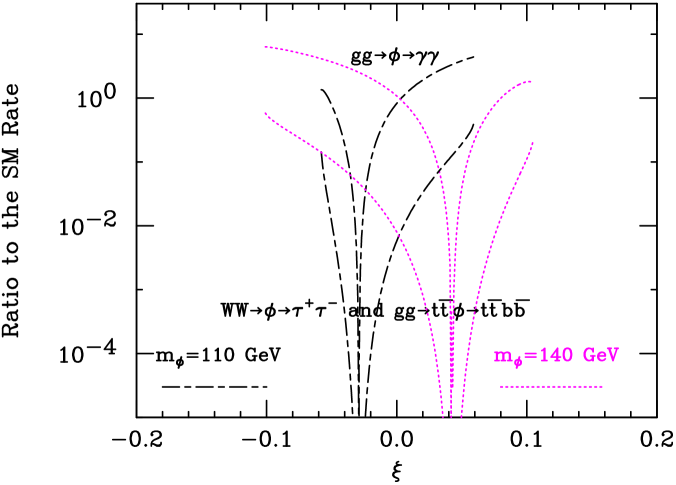
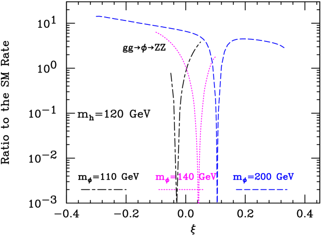
Figure 23: The ratio of the rates for $gg\to\phi\to\gamma\gamma$ (the higher curves for a given $m_{\phi}$) and for $WW\to\phi\to\tau^{+}\tau^{-}$ (the latter being the same as that for $gg\to t\overline{t}\phi\to t\overline{t}b\overline{b}$) to the corresponding rates for the SM Higgs boson. Results are shown for $m_{h}=120\;\hbox{GeV}$ and $\Lambda_{\phi}=1\;\hbox{TeV}$ as functions of $\xi$ for $m_{\phi}=110$ and $140\;\hbox{GeV}$.

Figure 24: The ratio of the rate for $gg\to\phi\to ZZ$ to the corresponding rate for a SM Higgs boson with mass $m_{\phi}$ assuming $m_{h}=120\;\hbox{GeV}$ and $\Lambda_{\phi}=1\;\hbox{TeV}$ as a function of $\xi$ for $m_{\phi}=110$, $140$ and $200\;\hbox{GeV}$. Recall that the $\xi$ range is increasingly restricted as $m_{\phi}$ becomes more degenerate with $m_{h}$.

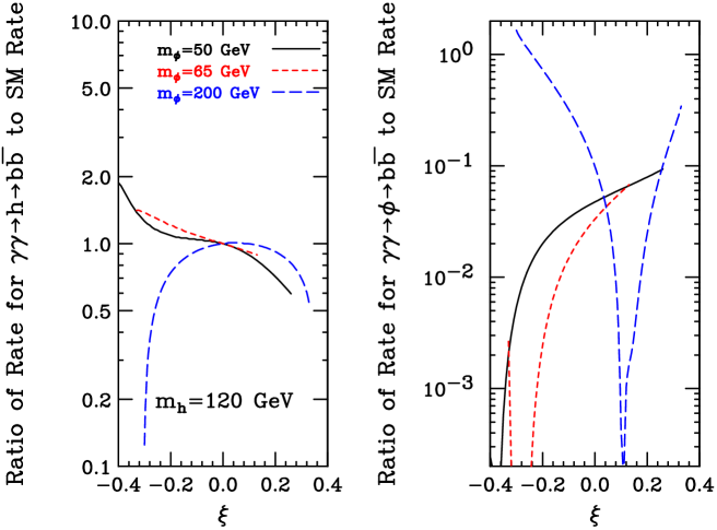
Figure 25: The rates for $\gamma\gamma\to h\to b\overline{b}$ and $\gamma\gamma\to\phi\to b\overline{b}$ relative to the corresponding rate for a SM Higgs boson of the same mass. Results are shown for $m_{h}=120\;\hbox{GeV}$ and $\Lambda_{\phi}=1\;\hbox{TeV}$ as functions of $\xi$ for $m_{\phi}=50$, $65$ and $200\;\hbox{GeV}$.

Next, we present the corresponding graphs related to LHC and $\gamma\gamma$ collider discovery. For these graphs, we have chosen to focus on $m_{h}=120\;\hbox{GeV}$ (as for $\Lambda_{\phi}=5\;\hbox{TeV}$) and on the values of $m_{\phi}=50$, $65$ and $200\;\hbox{GeV}$. The lowest value still gives a substantial range of allowed $\xi$ and will have significant $BR(h\to\phi\phi)$. For the middle value, these decays are forbidden. In all the LHC and $\gamma\gamma$ collider graphs, $m_{1}$ is assumed to be large, in particular large enough that decays of the Higgs or radion to $h^{1}$ are forbidden. The main implication of Figs. 22, 22, 24, 24 and 25 is that for $\Lambda_{\phi}=1\;\hbox{TeV}$, $\phi$ discovery at the LHC and in $\gamma\gamma$ collisions has much better prospects (away from the usual zeroes in the $\phi gg$ and $\phi\gamma\gamma$ couplings) than in the case of $\Lambda_{\phi}=5\;\hbox{TeV}$. It is still true that the anomalous contributions to the $h\gamma\gamma$ and $\phi\gamma\gamma$ couplings will be hard to isolate.

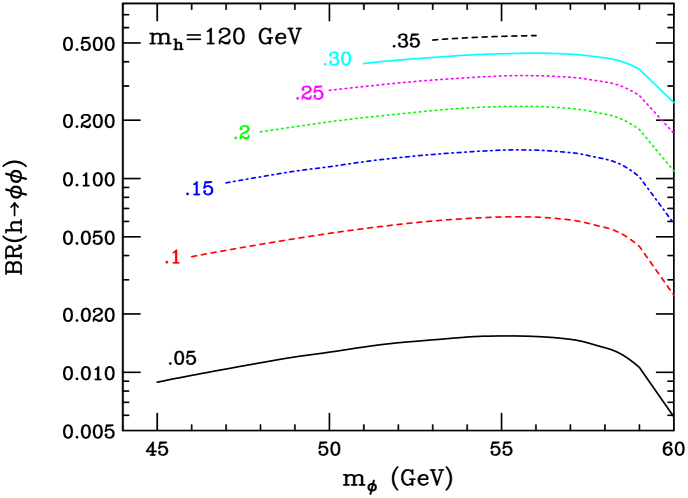
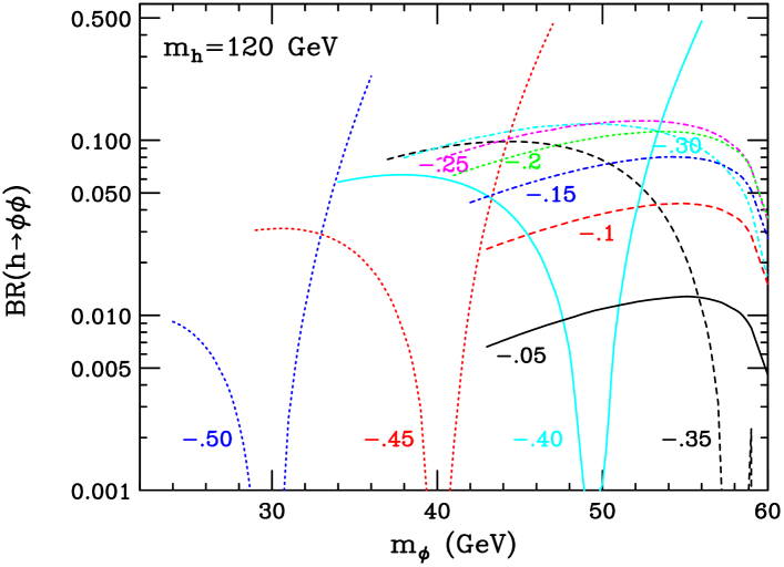
Figure 26: For various $\xi>0$ and $\xi<0$ values, the branching ratio for $h\to\phi\phi$ is plotted as a function of $m_{\phi}$, taking $m_{h}=120\;\hbox{GeV}$ and $\Lambda_{\phi}=1\;\hbox{TeV}$. Only points not excluded by LEP/LEP2 (the blue region of Fig. 18) are plotted. The curves terminate at low $m_{\phi}$ when the LEP/LEP2 limits of are encountered.

The greatest interest in the lower $\Lambda_{\phi}$ value derives from the fact that $h\to\phi\phi$ decays can be much more prominent and that $h,\phi$ decays to final states containing the 1st KK excitation $h^{1}$ become possible. The first point is illustrated in Fig. 26. $BR(h\to\phi\phi)$ can be as large as 50% at the highest allowed $|\xi|$ values.

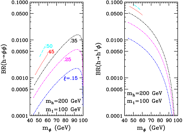
Figure 27: The $h\to\phi\phi$ and $h\to h^{1}\phi$ branching ratios as a function of $m_{\phi}$ for $m_{h}=200\;\hbox{GeV}$, $m_{1}=100\;\hbox{GeV}$, and $\Lambda_{\phi}=\sqrt{3}\widehat{\Lambda}_{W}=1\;\hbox{TeV}$, for various $\xi$ choices. Results are plotted only for $m_{\phi}$ values satisfying LEP/LEP2 bounds (the blue region of Fig. 18). The curve legend for the right-hand plot is the same as shown in the left-hand plot.

Let us now discuss what happens at higher $m_{h}$ values. The largest value that can be easily consistent with precision electroweak constraints is $m_{h}=200\;\hbox{GeV}$. For this value, we will require in our plots that $g_{ZZh}^{2}<1.2$ in order to be certain that $S,T$ lie within the 95% CL ellipse. In order to learn if the $h\to h^{1}\phi$ decay could be significant, we retain $\Lambda_{\phi}=1\;\hbox{TeV}$, for which Eq. (43) implies that $\widehat{\Lambda}_{W}=\Lambda_{\phi}/\sqrt{3}=577\;\hbox{GeV}$, and choose $m_{1}=100\;\hbox{GeV}$ [corresponding to $m_{0}/M_{Pl}\sim 0.065$, see Eq. (43)]. Results for $BR(h\to\phi\phi)$ and $BR(h\to h^{1}\phi)$ are plotted in Fig. 27 as a function of $m_{\phi}$ for selected values of $\xi>0$. (Only relatively small values of $|\xi|$ are not excluded by the $g_{ZZh}^{2}<1.2$ requirement when $\xi<0$.) The $h\to\phi\phi$ branching ratio can be significant, especially for the larger values of $\xi$ allowed by the theoretical constraint of $Z^{2}>0$. Certainly, these decays should be searched for at the LC as their presence would imply non-zero $\xi$ and would allow a measurement of this very fundamental parameter. The reason for the small size of the $h\to\phi\phi$ and $h\to h^{1}\phi$ branching ratios is the dominance of the $WW$ and $ZZ$ decay modes. Once these $VV$ decays become full strength, the $\phi\phi$ and $h^{1}\phi$ decays will be rare.

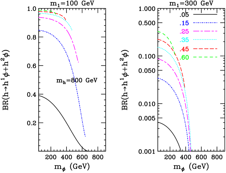
Figure 28: We plot the $h\to h^{1}\phi+h^{2}\phi$ branching ratio as a function of $m_{\phi}$ for $m_{h}=800\;\hbox{GeV}$ and $\Lambda_{\phi}=\sqrt{3}\widehat{\Lambda}_{W}=1\;\hbox{TeV}$, in the cases of $m_{1}=100\;\hbox{GeV}$ and $300\;\hbox{GeV}$, for various $\xi$ choices (as indicated in the right-hand window). Results are plotted only for $m_{\phi}$ values satisfying LEP/LEP2 bounds. In this plot, we have assumed that $h\to h^{1}h^{1}+\ldots$ decays (for which vertices do exist but have not been studied in detail in this paper) are unimportant even though they are kinematically allowed for the $m_{h}$ and $m_{1}$ choices of this figure.

As noted earlier, at still larger values of $m_{h}$ precision electroweak constraints become difficult to satisfy. A future paper will explore this region in more detail. Very roughly, the $\Gamma(h\to h^{n}\phi)\sim\widehat{\Lambda}_{W}^{-2}m_{h}^{7}/m_{n}^{4}$ behavior found earlier in Eq. (63) means that $h\to h^{n}\phi$ decays can dominate over the $WW$ and $ZZ$ decay modes that grow only as $m_{h}^{3}$, provided that $m_{1}$ is sufficiently small and that $\widehat{\Lambda}_{W}$ (and hence $\Lambda_{\phi}$) is of order a TeV. To illustrate, in Fig. 28 we plot $BR(h\to h^{1}\phi+h^{2}\phi)$ for $m_{h}=800\;\hbox{GeV}$ as a function of $m_{\phi}$ for a number of positive $\xi$ values and for the cases of $m_{1}=100\;\hbox{GeV}$ and $m_{1}=300\;\hbox{GeV}$. [$BR(h\to\phi\phi)$ is typically below or of order 0.01 for this large a value of $m_{h}$.] In obtaining the results shown, we have assumed that $h\to h^{1}h^{1}+\ldots$ decays (for which vertices do exist but have not been studied in detail in this paper) are unimportant even though they are kinematically allowed for the $m_{h}$ and $m_{1}$ choices of this figure. We also note that $BR(h\to h^{1}\phi)>11BR(h\to h^{2}\phi)$ for the cases studied, as anticipated from the $(m_{1}/m_{2})^{4}\sim(3.8/7)^{4}\sim 0.086$ scaling noted above. From Fig. 28, we see that $m_{1}=100\;\hbox{GeV}$ yields large values of $BR(h\to h^{1}\phi+h^{2}\phi)$ at small $m_{\phi}$ when $\xi$ is not small. For $m_{1}=300\;\hbox{GeV}$, $BR(h\to h^{1}\phi+h^{2}\phi)$ is much smaller than for $m_{1}=100\;\hbox{GeV}$, being of order $\sim 0.04\div 0.4$ for small values of $m_{\phi}$ and $\xi$ ranging from 0.05 to 0.60. Results for $\xi<0$ are very similar in nature.

6 Summary and Conclusions

We have discussed the scalar sector of the Randall-Sundrum model. The effective potential (defined as a set of interaction terms that contain no derivatives) for the Standard Model Higgs-boson ($h_{0}$) sector interacting with Kaluza-Klein excitations of the graviton ($h_{\mu}^{\mu\,n}$) field and the radion ($\phi_{0}$) field has been derived. Without specifying its origin, a stabilizing mass-term for the radion has been introduced. After including this term, we have shown that only the Standard Model vacuum determined by $\partial V(h_{0})/\partial h_{0}=0$ is allowed. Further, we find that consistency of the RS solution requires that the Higgs potential vanishes at the vacuum solution. Otherwise, the finely tuned matching required in the RS model between the bulk and branes would be violated. As a result, for the correct vacuum solution the effective potential does not contain any terms linear in the quantum Higgs field. The above results emerge only with a very full treatment of the effective potential. Truncation of its expansion in powers of the fields can lead to erroneous conclusions.

Having confirmed that the usually assumed vacuum properties are correct, we pursue in more detail the phenomenology of the RS scalar sector, focusing in particular on results found in the presence of a curvature-scalar mixing $\xi\,R\,\widehat{H}^{\dagger}\widehat{H}$ contribution to the Lagrangian. We delineate the somewhat tricky ‘inversion’ procedure for determining all the Lagrangian parameters given the masses of the physical eigenstates $h$ and $\phi$. A full set of Feynman rules for the resulting tri-linear interactions among the $h$, $\phi$ and $h^{n}$ mass eigenstates are then derived. We also summarize the Feynman rules for couplings to standard channels: $b\overline{b},WW,\ldots$ as well as $gg$ and $\gamma\gamma$ (including the anomalous contributions to the latter). Simple sum rules that relate Higgs-boson and radion couplings to pairs of vector bosons and fermions are given. Of particular interest is the fact that non-zero $\xi$ induces interactions linear in the Higgs field: $\phi^{2}h$ and $h^{n}h\phi$. The explicit forms of these interactions must be obtained using the above-mentioned full treatment of the effective potential as well as a similarly full treatment of the related derivative terms in the Lagrangian.

We summarize the connections between the parameters of the model and the lower bounds on the new physics scales among these parameters required by precision electroweak and Tevatron RunI constraints. We explore the behavior of the couplings in the range of parameter space allowed by theoretical and existing experimental constraints. In particular, we derive the regions of parameter space that are excluded by direct LEP/LEP2 limits on scalar particles with $ZZ$ coupling as function of scalar mass. Of particular note is the fact that the sum rule for $ZZh$ and $ZZ\phi$ squared-couplings noted above implies that it is impossible for both the $h$ and $\phi$ to be light.

We note that precision electroweak data is most naturally satisfied if the $h$ and $\phi$ masses are modest in size, $\mathrel{\raise 1.29167pt\hbox{$<$\kern-7.5pt\lower 4.30554pt\hbox{$\sim$}}}200\;\hbox{GeV}$. We focus on the case of small to moderate $m_{h}$ and $m_{\phi}$, and discuss expectations for $h$ and $\phi$ production/detection at the LHC and a LC in comparison to the SM Higgs boson. In the regions of parameter space allowed by theoretical and current experimental constraints, we find that LHC detection of the $\phi$ is likely to be quite difficult. In addition, LHC detection of the $h$ is not guaranteed.

One particularly interesting complication for $\xi\neq 0$ is the presence of the non-standard decay channel $h\to\phi\phi$. The $h\to\phi\phi$ decay could easily be present since in the context of the RS model there is a possibility (perhaps even a slight preference) for the $\phi$ to be substantially lighter than the $h$. In particular, $m_{\phi}<m_{h}/2$ is a distinct possibility. We study in detail the phenomenology when $m_{\phi}\leq 60\;\hbox{GeV}$ for $m_{h}=120\;\hbox{GeV}$, for which $h\to\phi\phi$ is possible.

In the main phenomenology section, Sec. 4, we consider the new physics scales of $\Lambda_{\phi}=5\;\hbox{TeV}$ and $m_{1}\sim 750\;\hbox{GeV}$ for the first KK resonance, $h^{1}$. These values imply that constraints from precision electroweak data and from RunI Tevatron data are clearly satisfied. For this case, the $h\to h^{1}\phi+\ldots$ modes, which are also potentially very interesting, are forbidden for the moderate $m_{h}$ and $m_{\phi}$ values explored here.

For $m_{h}=120\;\hbox{GeV}$, for the largest allowed $|\xi|$ values and for $m_{\phi}$ close to $m_{h}/2$, the $h\to\phi\phi$ mode will substantially dilute the rates for the usual search channels. In fact, we find that $BR(h\to\phi\phi)$ could easily be as large as $30\div 40\,\%$. Regardless of the magnitude of $BR(h\to\phi\phi)$, detection of this decay would be very important as it provides a crucial experimental signature for non-zero $\xi$.

Of course, it is also possible that $m_{\phi}>2m_{h}$. Because of the typically large size of the $\phi hh$ coupling, we find that $\phi\to hh$ decays will have a large branching ratio even when $m_{\phi}>2m_{W}$.

We give additional details regarding direct detection of the $\phi$ for the portion of parameter space for which $h\to\phi\phi$ decays are important. Prospects for direct detection at the LHC are not encouraging. At the LC, one should be able to detect $e^{+}e^{-}\to Z\phi$ using the recoil mass technique; $b$-tagging is not necessarily reliable due to the possibility that $\phi$ decays will be dominated by the $gg$ mode.

In addition to the above, we give a first assessment of whether or not the anomalous contribution to the $hgg$, $h\gamma\gamma$, $\phi gg$ and $\phi\gamma\gamma$ couplings could be observed experimentally. Deviations in these couplings-squared due to the anomalous contribution are plotted and compared to the errors expected from the outlined experimental procedures for extracting such deviations. Prospects in the case of the $h$ are relatively encouraging.

In a second phenomenology section, Sec. 5, we consider the case of much lighter new physics scales set by $\Lambda_{\phi}=1\;\hbox{TeV}$. In this case, we consider both large $m_{1}$, which avoids precision EW and RunI constraints, but requires large five-dimensional curvature, and the small curvature values of $m_{1}=100\;\hbox{GeV}$ and $300\;\hbox{GeV}$. It is not clear if these latter cases are ruled out by precision electroweak and/or RunI Tevatron data. If such low scales are allowed, the $h\to\phi\phi$ branching ratio becomes even more prominent for our sample choice of $m_{h}=120\;\hbox{GeV}$. For $m_{h}=200\;\hbox{GeV}$ and above, $h\to h^{1}\phi$ decays rapidly emerge and become dominant for $m_{h}\mathrel{\raise 1.29167pt\hbox{$>$\kern-7.5pt\lower 4.30554pt\hbox{$\sim$}}}500\;\hbox{GeV}$ in the case of $m_{1}=100\;\hbox{GeV}$. However, it must be kept in mind that for such large $m_{h}$ values other new physics must compensate the consequent large precision electroweak contributions from the Higgs loop graphs.

Overall, the Randall-Sundrum scenario leads to a fascinating extension of the usual Higgs phenomenology, especially if radion-Higgs mixing is present, as is most naturally the case.

Note added. In the course of preparing this paper, another article appeared dealing with the variations of the couplings of the $h$ and $\phi$ and their branching ratios due to the curvature-scalar mixing [24].

ACKNOWLEDGMENTS

B.G. thanks Zygmunt Lalak, Krzysztof Meissner and Jacek Pawelczyk for useful discussions. J.F.G would like to thank J. Wells for useful discussions. B.G. is supported in part by the State Committee for Scientific Research under grant 5 P03B 121 20 (Poland). J.F.G. is supported by the U.S. Department of Energy and by the Davis Institute for High Energy Physics.

7 Appendix: Feynman Rules

In this Appendix, we summarize the relevant Feynman rules for the mass eigenstates $\phi$, $h$ and $h_{\mu\nu}^{n}$. Rules for the $VV$ couplings of the $\phi$ and $h$, the $f\overline{f}$ couplings of the $\phi$ and $h$, and the tri-linear self-couplings among the $\phi$, $h$ and $h_{\mu\nu}^{n}$ fields are given. We note that we are employing a normalization in which $\sum_{\mu\nu}[\epsilon_{\mu\nu}^{i}]^{*}\epsilon^{j\,\mu\nu}=2\delta^{ij}$. In this case, the spin sum for the $h_{\mu\nu}^{n}$ state polarizations is $\sum_{i=1,5}\epsilon_{\mu\nu}^{i}(k)\epsilon_{\rho\sigma}^{i\,*}(k)=B_{\mu\nu\rho\sigma}(k)$, where

$$B_{\mu\nu\rho\sigma}(k) = \left(\eta_{\mu\rho}-{k_{\mu}k_{\rho}\over m_{n}^{2}}\right)\left(\eta_{\nu\sigma}-{k_{\nu}k_{\sigma}\over m_{n}^{2}}\right)+\left(\eta_{\mu\sigma}-{k_{\mu}k_{\sigma}\over m_{n}^{2}}\right)\left(\eta_{\nu\rho}-{k_{\nu}k_{\rho}\over m_{n}^{2}}\right)$$ (69)

$$-{2\over 3}\left(\eta_{\mu\nu}-{k_{\mu}k_{\nu}\over m_{n}^{2}}\right)\left(\eta_{\rho\sigma}-{k_{\rho}k_{\sigma}\over m_{n}^{2}}\right)\,.$$

The parameters $a,b,c,d$ define the mixing between the $\xi=0$ states and the $\xi\neq 0$ mass eigenstates. They are defined in Eqs. (33) and (34). In the $\xi=0$ limit, $d=-a=1$, $c=b=0$. The auxiliary functions for the $gg$ and $\gamma\gamma$ couplings of the $h$ and $\phi$ (Fig. 29) are given by

$$F_{1/2}(\tau) = -2\tau[1+(1-\tau)f(\tau)]\,,$$ (70)

$$F_{1}(\tau) = 2+3\tau+3\tau(2-\tau)f(\tau)\,,$$ (71)

for spin-1/2 and spin-1 loop particles, respectively, with

$$f(\tau) = -{\textstyle{1\over 4}}\ln\left[-{1+\sqrt{1-\tau}\over 1-\sqrt{1-\tau}}\right]^{2}\,$$ (74)

$$= \left\{\begin{array}[]{cl}{\rm\arcsin}^{2}(1/\sqrt{\tau})\,,&\qquad\tau\geq 1\,,\\ -\frac{1}{4}\left[\ln\left(\frac{1+\sqrt{1-\tau}}{1-\sqrt{1-\tau}}\right)-i\pi\right]^{2}\,,&\qquad\tau\leq 1\,.\end{array}\right.$$

The variable $\tau$ for a given loop is defined as $\tau\equiv 4m^{2}/M^{2}$, where $m$ is the mass of the internal loop particle and $M$ is the mass of the scalar state, $h$ or $\phi$. In Fig. 30, the $\overline{g}$ couplings used in the branching ratio formulae, Eqs. (62) and (63), are defined. In the $\xi=0$ SM limit, $\overline{g}_{hhh}=-3m_{h}^{2}/v_{0}$ (where $m_{h}=m_{h_{0}}$ at $\xi=0$). We have not derived detailed results for the $hh^{n}h^{n}$ and $\phi h^{n}h^{n}$ couplings, although, as explained in the text, such couplings do exist.

Figure 29: Feynman rules for the $VV$ and $f\overline{f}$ couplings of the scalars $h$ and $\phi$. Note: Since there are no pseudoscalars, there are no single $V$ vertices. We have dropped the extra terms related to gauge fixing, see Ref. [9], as appropriate when considering on-shell $W$’s or $Z$’s or when working in the unitary gauge. For $gg,\gamma\gamma$ final states, we give only the on-shell rules. There, $\tau_{i}=4m_{i}^{2}/m_{h,\phi}^{2}$ where $m_{i}$ is the mass of the internal loop particle. The auxiliary functions for spin-1/2 and spin-1 loop particles are defined in the Appendix text. The SU(3)$\times$SU(2)$\times$U(1) $\beta$ function coefficients are $b_{3}=7$, $b_{2}=19/6$ and $b_{Y}=-41/6$. For $c_{g}$, the $\sum_{i}$ is over all colored fermions (assumed to have $N_{c}^{i}=3$). For $c_{\gamma}$, the $\sum_{i}$ comprises all charged fermions (including quarks, with $N_{c}^{i}=3$ and $e_{i}=2/3$ or $-1/3$, and leptons, with $e_{i}=-1$ and $N_{c}^{i}=1$) and the $W$ boson (with $e_{i}=1$ and $N_{c}^{i}=1$). For the $h$, $g_{fV}=g_{ZZh}=d+\gamma b$ and $g_{r}=\gamma b$. For the $\phi$, $g_{fV}=g_{ZZ\phi}=c+\gamma a$ and $g_{r}=\gamma a$.

Figure 30: Feynman rules for the tri-linear vertices in the scalar sector. All momenta are outward flowing. In the $h_{\mu\nu}^{n}$ vertices, we have made use of the symmetry of $h_{\mu\nu}^{n}$ under $\mu\leftrightarrow\nu$.

References

[1]
L. Randall, R. Sundrum,
Phys. Rev. Lett. 83, 3370 (1999), hep-ph/9905221;
L. Randall, R. Sundrum,
Phys. Rev. Lett. 83, 4690 (1999), hep-th/9906064.
[2]
C. Csaki, M. Graesser, L. Randall and J. Terning,
Phys. Rev. D 62, 045015 (2000)
[arXiv:hep-ph/9911406].
[3]
S. B. Bae, P. Ko, H. S. Lee and J. Lee,
Phys. Lett. B 487, 299 (2000)
[arXiv:hep-ph/0002224].
[4]
H. Davoudiasl, J. L. Hewett and T. G. Rizzo,
Phys. Rev. Lett. 84, 2080 (2000)
[arXiv:hep-ph/9909255].
[5]
K. Cheung,
Phys. Rev. D 63, 056007 (2001)
[arXiv:hep-ph/0009232].
[6]
H. Davoudiasl, J. L. Hewett and T. G. Rizzo,
Phys. Rev. D 63, 075004 (2001)
[arXiv:hep-ph/0006041].
[7]
S. C. Park, H. S. Song and J. Song,
Phys. Rev. D 63, 077701 (2001)
[arXiv:hep-ph/0009245].
[8]
G. Giudice, R. Rattazzi, J. Wells,
Nucl. Phys. B 595, 250 (2001), hep-ph/0002178.
[9]
C. Csaki, M.L. Graesser, G.D. Kribs,
Phys. Rev. D 63, 065002-1 (2001), hep-th/0008151.
[10]
T. Han, G. D. Kribs and B. McElrath,
Phys. Rev. D 64, 076003 (2001)
[arXiv:hep-ph/0104074].
[11]
M. Chaichian, A. Datta, K. Huitu and Z. h. Yu,
Phys. Lett. B 524, 161 (2002)
[arXiv:hep-ph/0110035].
[12]
W. D. Goldberger and M. B. Wise,
Phys. Rev. Lett. 83, 4922 (1999), hep-ph/9907447.
[13]
C. Charmousis, R. Gregory and V. A. Rubakov,
Phys. Rev. D 62, 067505 (2000), hep-th/9912160.
[14]
J.J. van der Bij,
Acta Phys. Polon. B 25, 827 (1994);
R. Raczka, M. Pawlowski,
Found. Phys. 24, 1305 (1994), hep-th/9407137.
[15]
G. D. Kribs,
in Proc. of the APS/DPF/DPB Summer Study on the Future of Particle Physics (Snowmass 2001) ed. R. Davidson and C. Quigg,
arXiv:hep-ph/0110242.
[16]
R. Delbourgo and D.S. Liu,
Austral. J. Phys. 53, 647 (2001)
[arXiv:hep-ph/0004156].
[17]
G. Abbiendi et al. [OPAL Collaboration],
Eur. Phys. J. C 7, 407 (1999), hep-ex/9811025.
[18]
D. Buskulic et al. [ALEPH Collaboration],
Phys. Lett. B 313, 312 (1993).
[20] LEP seminar, July 10, 2001, P Teixeira-Dias,
on behalf of the LEPHIGGS working group.
[21]
[LEP Higgs Working Group for Higgs boson searches Collaboration],
arXiv:hep-ex/0107029.
[22] A. Djouadi, J. Kalinowski, M. Spira, Comput. Phys.
Commun. 108, 46 (1998).
[23]
T. Abe et al. [American Linear Collider Working Group Collaboration],
in Proc. of the APS/DPF/DPB Summer Study on the Future of Particle Physics (Snowmass 2001) ed. R. Davidson and C. Quigg,
arXiv:hep-ex/0106056. See sections 8.5 and 8.6, and Table 3.2.
[24]
J. L. Hewett and T. G. Rizzo,
hep-ph/0202155.