Vacuum polarization energy losses of high energy cosmic rays.

Abstract

The process of the vacuum polarization energy losses of high energy cosmic rays propagating in the extragalactic space is considered. The process is due to the polarization of Cosmic Background Radiation by a moving charged particle. With the goal of the description of the process, the photon mass, refractive indices and permittivity function for low and high energy photons are found. Calculations show the rather noticeable level of the energy losses for propagating protons with the energies more than $10^{6}-10^{7}GeV$. The influence of the polarization energy losses on propagation of cosmic rays is discussed.

1 Introduction

The problems of the origin and propagation of high energy cosmic rays is widely discussed in recent years (see, for example [1, 2, 3] and literature therein). The photoproduction of mesons and $e^{\pm}$-pairs in the Cosmic Background Radiation was considered as the main reason of the energy losses of charged particles propagating in the extragalactic space[2, 4, 5]. However, the simulations of the spectral distributions of cosmic rays on this basis do not provide a close agreement with observed data [2], and some peculiarities in the spectrum like the ”knee” [6] and GZK-cutoff [7, 8] do not find recognized explanation. In this connection the determination of another reason of the energy losses is important and interesting.

In this paper we consider the possible mechanism by which cosmic rays lose their energy in the extragalactic space. It is the polarization energy losses of a charged particle moving in the electromagnetic vacuum. In the presence of an external electromagnetic field the polarization of vacuum was considered first in the pioneer papers [9]. The vacuum polarization leads to different effects [10] such as the nonlinearity of the Maxwell equations, appearance of nonzero photon mass, birefringence of light, etc. The description of the various methods in the QED of vacuum one can find in literature ( see [11] and references therein). In parallel with other methods the traditional method, based on the introduction of the permittivity tensor, may be used for the effective description of different phenomena in the electromagnetic vacuum. In this case the vacuum described by the Maxwell equations which are similar to equations of the classical electrodynamics for continuous media[12, 13]. As an example, one can point out the well known low energy permittivity and permeability tensors for constant electric and magnetic fields [10]. In paper [14] the connection between the polarization and permittivity tensors is established. The using of the permittivity tensor is convenient because this approach allows to consider the QED vacuum and matter with the unit point of view.

2 The mass of photon, propagating in an isotropic photon gas

The photon mass $m_{\gamma}$ in an isotropic medium is defined by the refractive index $\tilde{n}$ of monochromatic photons propagating in this medium

$$m_{\gamma}^{2}c^{4}=2E_{\gamma}^{2}(1-\tilde{n}(E_{\gamma}))$$ (1)

where $E_{\gamma}$ is the photon energy. From this equation one can see the equivalence of finding of the photon mass and the refractive index. Note that in the general case the refractive index is a complex value. However, in a transparent medium its imaginary part is a negligibly small quantity.

Our calculations of photon mass in an isotropic photon gas are based on the results of papers [15, 16], where propagation of $\gamma$-quanta in the field of monochromatic and dichromatic laser waves was considered. In these papers the permittivity tensor was derived for such media. Knowing this tensor one can find the refractive indices of photon and other characteristics of the propagation process. The imaginary components of the tensor are connected with the energy losses due to $e^{\pm}$-pair production in the laser wave. The real components of the permittivity tensor are derived with the help of dispersion relations. In the case of an isotropic photon gas the energy losses one can describe by the following relation (see, for example[17]):

$$L_{\gamma\gamma}^{-1}(E_{\gamma})={1\over{8E_{\gamma}^{2}}}\int_{\epsilon_{min}}^{\infty}{d\epsilon{n(\epsilon)\over\epsilon^{2}}\int_{s_{min}}^{s_{max}}{\sigma_{\gamma\gamma}sds}}$$ (2)

where $\L_{\gamma\gamma}$ is the reciprocal of the mean free path for collisions, $n(\epsilon)$ is the differential photon gas number density for the photon energy equal to $\epsilon$, $s$ is the center of momentum frame energy squared, $\sigma_{\gamma\gamma}(s)$ is the total cross section of $e^{\pm}$-pair production, $E_{\gamma}$ is the energy of photon propagating in a medium, $s_{min}=4m^{2}c^{4}$, $s_{max}=4\epsilon E_{\gamma}$, $\epsilon_{min}=s_{min}/4E_{\gamma}$, m is the electron mass and $c$ is the speed of light in the vacuum. All relations in this paper will be valid for the laboratory coordinate system, which determined as the system where the mean momentum of the background photons is equal to zero. From Eq.(2) one can find the imaginary part of refractive index $\tilde{n}$

$$Im(\tilde{n}(E_{\gamma}))={{L_{\gamma\gamma}^{-1}\hbar c}\over{2E_{\gamma}}}$$ (3)

The explicit form of this relation is:

$$Im(\tilde{n}(E_{\gamma}))={{\pi r_{e}^{2}\lambda_{e}}\over{mc^{2}}}\int_{\epsilon_{min}}^{\infty}{{\cal{F}}_{im}(z_{m})n(\epsilon)\epsilon d\epsilon},$$ (4)

$${\cal{F}}_{im}(z_{m})=z_{m}^{3}\int_{z_{m}}^{1}{[(1+z-z^{2}/2)\ln{{1+\sqrt{1-z}}\over{1-\sqrt{1-z}}}-\sqrt{1-z}(1+z)}]{dz\over z^{2}}$$ (5)

where $r_{e}$ and $\lambda_{e}$ are the classical radius of electron and its Compton wavelength, $z=4m^{2}c^{4}/s$ and $z_{m}=4m^{2}c^{4}/s_{max}=m^{2}c^{4}/(\epsilon E_{\gamma})$. The corresponding real part of the photon refractive index is:

$$Re(\tilde{n}(E_{\gamma}))-1={{2r_{e}^{2}\lambda_{e}}\over{mc^{2}}}\int_{0}^{\infty}{{\cal{F}}_{re}(z_{m})n(\epsilon)\epsilon d\epsilon},$$ (6)

where function ${\cal{F}}_{re}(z)$ is determined by the following relation:

$${\cal{F}}_{re}(z_{m})=z_{m}^{3}\int_{z_{m}}^{\infty}\Phi(z){dz\over z^{2}}$$ (7)

$$\Phi(z)=\cases{-3-(1+z-{z^{2}\over 2}){1\over 4}L^{2}_{-}-(1-(z+{z^{2}\over 2})){1\over 4}L^{2}_{+}+\cr+{{(1+z)\sqrt{1-z}}\over{2}}L_{-}-{{(z-1)\sqrt{z+1}}\over{2}}L_{+}+{\pi^{2}\over 4}(1+z-{{z^{2}}\over 2}),\;0<z\leq 1,\cr-3+(1+z-{z^{2}\over 2})\mathop{\rm arccot}\nolimits^{2}(\sqrt{z-1})-(1-(z+{z^{2}\over 2})){1\over 4}L^{2}_{+}+\cr+(1+z)\sqrt{z-1}\mathop{\rm arccot}\nolimits\sqrt{z-1}-{{(z-1)\sqrt{1+z}}\over{2}}L_{+},\;z>1.\cr}$$ (8)

The functions $L_{-},\,L_{+}$ are equal to:

$$L_{-}=\ln{{1+\sqrt{1-z}}\over{1-\sqrt{1-z}}},\quad L_{+}=\ln{{\sqrt{1+z}+1}\over{\sqrt{1+z}-1}}.$$

The obtained here relations for refractive indices are valid for low and high energy photons propagating in a photon gas. Now one can calculate the refractive indices of the photon propagating in the extragalactic space. As the first approximation of this medium one can take the model of the space which is filled by the Cosmic Background Radiation. In this case the number density is defined by well known equation:

$$n(\epsilon)d\epsilon={1\over{\pi^{2}c^{3}\hbar^{3}}}{{\epsilon^{2}d\epsilon}\over{\exp(\epsilon/T)-1}}\,,$$ (9)

where $T$ is the temperature. For low energy photons one can find the following relation for real part of the refractive index:

$$Re(\tilde{n}(0))-1={{44r_{e}^{2}\lambda_{e}}\over{135mc^{2}}}\int_{0}^{\infty}{n(\epsilon)\epsilon d\epsilon}={{44\pi^{2}\alpha^{2}}\over 2025}{{T^{4}}\over{m^{4}c^{8}}}\,.$$ (10)

The real and imaginary parts of refractive indices are connected by the dispersion relation:

$$Re(\tilde{n}(E_{\gamma}))-1={2\over\pi}{\cal{P}}\int_{0}^{\infty}{{\hat{E}_{\gamma}Im(\tilde{n}(\hat{E_{\gamma}}))d\hat{E}_{\gamma}}\over{\hat{E}_{\gamma}^{2}-E_{\gamma}^{2}}}$$ (11)

At present temperature $T=2.726^{o}\,K$ the real part of refractive index for low energy photons is $5.1\,10^{-43}$. These results are in agrement with the similar calculations [18, 19, 20] of the low energy refractive indices in an isotropic photon gas.

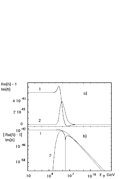
Figure 1: The real minus unit (1) and imaginary (2) parts of refractive index (in linear (a) and logarithmic (b) scales) in Cosmic Background Radiation as functions of the photon energy. The absolute value $|Re{\tilde{n}}-1|$ is shown in logarithmic scale.

Fig.1 illustrates the results of calculation of the photon refractive indices in the simplest model of the extragalactic medium (in the Cosmic Background Radiation). One can see that the real part is nearly constant in the wide energy range from 0 till $2\,10^{5}$ GeV with the flat maximum ($\approx 6\,10^{-43}$) at $E_{\gamma}\approx 3\,10^{5}GeV$. At energies more than $2.5\,10^{6}GeV$ the real part of index is negative. The imaginary part has maximum value $\approx 4\,10^{-43}$ at $E_{\gamma}=8\,10^{5}GeV$.

Knowing the refractive indices one can find the energy dependence of the permittivity function of a photon gas. However, this function is not uniquely defined and it depends on the relation between magnetic induction vector $B$ and intensity of magnetic field $H$ (see [12, 13]). In [15] the Maxwell equations are written with $H=B$ and in this case the permittivity function $\varepsilon$ is

$$\varepsilon(E_{\gamma})=\tilde{n}^{2}\approx 1+2Re(\tilde{n}-1)+2iIm(\tilde{n}).$$ (12)

3 Energy losses of particle moving in a medium

Propagating in the Cosmic Background Radiation charged cosmic rays produce polarization of this medium. As result the cosmic rays lose the initial energy. This process is similar in many respects to the ionization losses of energy of charged particles moving in matter. It is clear that the vacuum polarization is many times more weak process, however it may be noticeable on a large distances of particle propagation in such a specific medium as the extragalactic space.

Our consideration will be based on the Landau theory of ionization energy losses of relativistic particles in a matter [12]. However, a small adaptation of the theory will be done with the goal of the elimination of divergences in the final result.

The Maxwell equations in a medium have the following form:

$$\mathop{\rm div}\nolimits{{\bf{B}}}=0,\qquad\mathop{\rm rot}\nolimits{{\bf{E}}}=-{1\over c}{\partial{{\bf{B}}}\over\partial{t}},$$ (13)

$$\mathop{\rm div}\nolimits{\hat{\varepsilon}{\bf{E}}}=4\pi\rho,\,\,\,\mathop{\rm rot}\nolimits{{\bf{B}}}={1\over c}{\partial{\hat{\varepsilon}}{\bf{E}}\over\partial{t}}+{4\pi\over c}{\bf{j}}.$$ (14)

where ${\bf{E}}$ is the intensity of electric field and $\bf{B}$ is the magnetic induction vector, $\rho$ and ${\bf{j}}$ are the charge and current densities, $\hat{\varepsilon}$ is the permittivity operator (see[12]), t is the time.

The charge and current distributions one can take in the following form:

$$\rho=e\rho({\bf{r}}-{\bf{v}}t),\quad{\bf{j}}=e\rho({\bf{r}}-{\bf{v}}t){\bf{v}},\qquad\int_{V}{\rho(\bf{r})d{\bf{r}}}=1,$$ (15)

where $e$ is the particle charge. The field potentials we write in the usual form:

$${\bf{B}}=\mathop{\rm rot}\nolimits{{\bf{A}}},\qquad{\bf{E}}=-{1\over c}{\partial{{\bf{A}}}\over\partial{t}}-\mathop{\rm grad}\nolimits\varphi$$ (16)

In accordance with [12] we use the further condition for potentials:

$$\mathop{\rm div}\nolimits{{\bf{A}}}+{1\over c}{\partial{\hat{\varepsilon}}\varphi\over\partial{t}}=0.$$ (17)

The substitution Eq(17) in Eq(15) allows to get the following relations for potentials:

$$\Delta{\bf{A}}-{\hat{\varepsilon}\over c^{2}}{\partial^{2}{\bf{A}}\over\partial{t^{2}}}=-{4\pi\over c}e\rho({\bf{r}}-{\bf{v}}t){\bf{v}},$$ (18)

$$\hat{\varepsilon}(\Delta\varphi-{\hat{\varepsilon}\over c^{2}}{\partial^{2}\varphi\over\partial{t^{2}}})=-4\pi e\rho({\bf{r}}-{\bf{v}}t).$$ (19)

These equations for Fourier components have the form:

$$k^{2}{\bf{A_{k}}}+{\hat{\varepsilon}\over c^{2}}{\partial^{2}{{\bf{A_{k}}}}\over\partial{t^{2}}}={4\pi\over c}eF_{\bf{k}}{\bf{v}}\exp({-i{\bf{kv}}t}),$$ (20)

$$\hat{\varepsilon}(k^{2}\varphi_{\bf{k}}+{\hat{\varepsilon}\over c^{2}}{\partial^{2}\varphi_{\bf{k}}\over\partial{t^{2}}})=4\pi eF_{\bf{k}}\exp{(-i{\bf{kv}}t)}.$$ (21)

where $F_{\bf{k}}=\int{\rho({\bf{r}})\exp({-i{\bf{kr}}})d{\bf{r}}}$. One can see that the functions ${\bf{A_{k}}}$ and $\varphi$ depend on the time as $\exp{(-i{\bf{kv}})}$. As it shown in [12], the result of action of $\hat{\varepsilon}$-operator on $\exp{(-i\omega t)}$- function is its multiplication on $\varepsilon(\omega)$-function. Now from Eqs.(21-22) one can get:

$${\bf{A_{k}}}={4\pi e\over c}\,{F_{\bf{k}}{\bf{v}}\over k^{2}-{(\bf{kv}})^{2}\varepsilon({{\bf{kv}}})/c^{2}}\exp{(-i{\bf{kv}}t)},$$ (22)

$$\varphi_{\bf{k}}={4\pi e\over\varepsilon({{\bf{kv}})}}\,{F_{\bf{k}}\over k^{2}-{(\bf{kv}})^{2}\varepsilon({{\bf{kv}}})/c^{2}}\exp{(-i{\bf{kv}}t)}.$$ (23)

The Fourier component of the intensity of electric field has the following form:

$${\bf{E_{k}}}={i{\bf{kv}}\over c}{\bf{A_{k}}}-i{\bf{k}}\varphi_{\bf{k}}.$$ (24)

Now we find the damping force, which act on the extended charge. For this purpose we use the following well known relation:

$${d\over dt}({{\bf{DE}}+B^{2}\over 8\pi})=-{\bf{jE}}-\mathop{\rm div}\nolimits{\bf{S}},\quad{\bf{S}}={c\over 4\pi}[{\bf{EB}}],$$ (25)

where $\bf{D}$ is the electrical induction vector. After integration over some volume $V$ one can get:

$${d{\cal{H}}\over dt}=-e{\bf{v}}\int_{V}{\rho({\bf{r}}){\bf{E}}({\bf{r}})d{\bf{r}}}-\oint_{\sigma}{S_{n}d\sigma},\qquad{\cal{H}}=\int_{V}{{{{{\bf{DE}}+B^{2}}\over 8\pi}\,dV}},$$ (26)

where $\sigma$ is the bounding surface. It is clear, that at ${\bf{r}}\rightarrow\infty$ the surface integral tends to zero. Then the damping force has the following form:

$${\bf{{\cal{F}}}}=-{e{\bf{v}}\over v}\int_{V}{\rho({\bf{r}}){\bf{E}}({\bf{r}})\,d{\bf{r}}}$$ (27)

Obviously that Fouirier component of electric intensity has the form: ${\bf{E_{k}}}={\bf{\Phi}}({\bf{k}})\exp{-i{\bf{kv}}t}$, where ${\bf{\Phi}}({\bf{k}})$ is the known function (see Eqs.(23-25)). Then we can write the following relation:

$$e{\bf{v}}\int_{V}{\rho({\bf{r}}-{\bf{v}}t){\bf{E}}\,d{\bf{r}}}=\qquad\qquad\qquad\qquad\qquad\qquad\quad$$ (28)

$${e{\bf{v}}\over(2\pi)^{3}}\int{\{\int_{V}\rho({\bf{r}}-{\bf{v}}t)\exp{i{\bf{k}}({\bf{r}}-{\bf{v}}t)}d{\bf{r}}\}\Phi({\bf{k}})d{\bf{k}}}={e{\bf{v}}\over(2\pi)^{3}}\int{F_{\bf{k}}{\bf{\Phi}}({\bf{k}})\,d{\bf{k}}},$$

Obviously, the damping force is directed against the velocity of particle. Let us name $k_{x}v=\omega$ and $q=\sqrt{k_{y}^{2}+k_{z}^{2}}$, where $x$-coordinate axis is along the direction of motion, $\omega$ is the photon frequency. Now one can obtain the following equation for the absolute value of the damping force:

$${\cal{F}}={ie^{2}\over\pi}\int_{-\infty}^{\infty}{\int_{0}^{\infty}{{F^{2}_{\bf{k}}(k)({1\over v^{2}}-{\varepsilon\over c^{2}})\omega q\,dqd\omega}\over{\varepsilon[q^{2}+\omega^{2}({1\over v^{2}}-{\varepsilon\over c^{2}})]}}}$$ (29)

One can see that these relation is differ from similar relation in [12] by $F^{2}(k)$-multiplier. This multiplier is the charge distribution of the moving particle in ${\bf{k}}$-space (the axial symmetry of the charge distribution around x-axis is assumed). For next we can write that $\varepsilon\approx 1+\Delta\varepsilon^{\prime}+i\Delta\varepsilon^{\prime\prime},\,|\Delta\varepsilon^{\prime}|<<1,\Delta\varepsilon^{\prime\prime}<<1$. Then we extract the real and imaginary parts of the integrand function in Eq.(30). Thus, we get the sum of two integrals: $I_{1}+iI_{2}$. Besides, it needs to take into account that $\Delta\varepsilon^{\prime}$ and $\Delta\varepsilon^{\prime\prime}$ are even and odd functions of the frequency. One can show that $I_{2}=0$, and therefore the damping force is:

$${\cal{F}}={2e^{2}\over\pi v^{2}}\int_{0}^{\infty}{\int_{0}^{\infty}{{F^{2}(q^{2}+{\omega^{2}\over v^{2}\gamma^{2}})\Delta{\varepsilon^{\prime\prime}}(\omega)(q^{2}+{\omega^{2}\over\gamma^{4}v^{2}})\omega q\,d\omega dq\over(q^{2}+{\omega^{2}\over v^{2}\gamma^{2}}-{\omega^{2}\Delta\varepsilon^{\prime}\over c^{2}})^{2}+{\omega^{4}\Delta\varepsilon^{\prime\prime 2}\over c^{4}}}}}$$ (30)

where $\gamma$ is the Lorentz factor of the particle. Besides, in this equation $F$ is the charge form factor of the particles (i.e. the charge distribution in ${\bf{k}}$-space in the particle rest frame). The Eq.(31) for the damping force is final. The two integrals in this equation are converged. The integral over $q$ is converged due to the form factor of the particle, and the integral over $\omega$ is converged due to relation:$\varepsilon\rightarrow 1$ at $\omega\rightarrow\infty$.

4 Energy losses of cosmic rays

For cosmic rays Eq.(31) one can simplify. It is well known that the maximum observed energy of cosmic rays is less than $10^{12}\,GeV$. One can see that energy losses depend on the real and imaginary parts of the permittivity function. However, one can neglect of this dependence in the denominator. It is really that $\gamma^{-2}>>|\Delta\varepsilon^{\prime}|,\,\Delta\varepsilon^{\prime\prime}$(see Fig.1 and [21]). Now one can write the damping force for cosmic rays in the following form:

$${\cal{F}}={2e^{2}\over\pi\hbar^{2}v^{2}}\int_{0}^{\infty}{\int_{0}^{\infty}{{F^{2}(\bar{q}^{2}+{E_{\gamma}^{2}\over v^{2}\gamma^{2}})\varepsilon^{\prime\prime}(E_{\gamma})(\bar{q}^{2}+{E\gamma^{2}\over v^{2}\gamma^{4}})E_{\gamma}\bar{q}\,dE_{\gamma}d\bar{q}\over(\bar{q}^{2}+{E_{\gamma}^{2}\over\gamma^{2}v^{2}})^{2}}}}\,$$ (31)

where $\bar{q}=\hbar q$ and $E_{\gamma}=\hbar\omega$. Here we use relation: $\varepsilon^{\prime\prime}=\Delta\varepsilon^{\prime\prime}$. For the next calculations we take the empirical electric proton form factor [22]:

$$F(Q)=(1+{Q^{2}\over M^{2}_{V}})^{-2}.$$ (32)

where $Q$ is the three-dimensional transfer momentum, the empirical constant $M^{2}_{V}=(0.84GeV/c)^{2}$. Then we find the integral over $\bar{q}$ and get the following relation:

$${\cal{F}}={e^{2}\over\pi\hbar^{2}v^{2}}\int_{0}^{\infty}{\varepsilon^{\prime\prime}(E_{\gamma})(S_{1}(E_{\gamma})+S_{2}(E_{\gamma}))E_{\gamma}\,dE_{\gamma}}\,$$ (33)

$$S_{1}(E_{\gamma})=-\ln(xy)-{y^{3}\over 3}-{y^{2}\over 2}-y,$$ (34)

$$S_{2}(E_{\gamma})=x({1\over\gamma^{2}}-1)(4\ln(xy)+{y^{3}\over 3}+y^{2}+3y+{1\over x}),$$ (35)

$$x={E_{\gamma}^{2}\over\gamma^{2}v^{2}M^{2}_{V}},\qquad\qquad\qquad\qquad y={1\over 1+x}.$$ (36)

It is helpful to obtain the inexact but simple estimation relation for the damping force. It is possible to make for the large $\gamma$-factors $(>10^{8})$ of the cosmic rays. This relation is:

$${\cal{F}}\sim{e^{2}\over\pi\hbar^{2}v^{2}}\ln({\gamma M_{V}v\over<E_{\gamma}>})\int_{0}^{E_{\gamma,b}}{\varepsilon^{\prime\prime}(E_{\gamma})E_{\gamma}dE_{\gamma}}$$ (37)

where $<E_{\gamma}>$ is some value of the $\gamma$-quantum energy range, where the integrand has noticeable quantities, $E_{\gamma,b}$ is the boundary value of the energy range and it is satisfied the condition $E_{\gamma,b}\gg\gamma M_{V}v$. For example, one can define the $\bar{E_{\gamma}}$ by the following equation:

$$\bar{E_{\gamma}}=\int_{0}^{E_{\gamma,b}}{\varepsilon^{\prime\prime}(E_{\gamma})E_{\gamma}dE_{\gamma}}\,\,/\,\,\int_{0}^{\infty}{\varepsilon^{\prime\prime}(E_{\gamma})dE_{\gamma}}.$$ (38)

According to calculations $<E_{\gamma}>\approx 8\,10^{7}GeV$ and the quantity of the integral in the numerator of Eq.(39) is equal to $\approx 10^{-28}GeV^{2}$ at $E_{\gamma,b}\sim 10^{13}\,GeV$. The choice of $E_{\gamma,b}$ in the energy range from $10^{10}$ till $10^{14}\,GeV$ is weakly changed the result. Then we get the following estimation:

$${\cal{F}}\sim{\alpha Z^{2}\over\pi\hbar c}10^{-28}\ln{\gamma M_{V}c\over<E_{\gamma}>},$$ (39)

where $Z$ is the particle charge in the elementary one units. From here one can see that energy losses of high energy cosmic rays (protons) is about some hundreds of GeV per light year. This value is the same order as the $e^{\pm}$-pair production in the Cosmic Background Radiation. Fig.2 illustrates the calculation of vacuum polarization energy losses of protons in accordance with Eq.(34).

5 Discussion

The results of calculations of the vacuum polarization energy losses of the high energy cosmic rays show that losses are reasonably large, and, because of this, it is necessary to take into account this process for true description of the particle propagation in the extragalactic space. Fig.3 illustrates the relative polarization energy losses of protons and iron nuclei in the extragalactic space. The results of calculation [2] of the energy losses due to the photoproduction processes ($p\,+\,\gamma\rightarrow\,p\,+\,e^{+}\,+\,e^{-},\,p\,+\,\gamma\rightarrow\,p\,+\,\pi^{0},...$) are also shown on the figure. One can see the following peculiarities of the considered process:

i) the spectral distribution of polarization energy losses are rather broad, and the flat maximum of the relative losses is at $E_{p,max}\approx 4\,10^{7}GeV$ and $E_{Fe,max}\approx 1.4\,10^{10}GeV$ for protons and iron nuclei, correspondingly;

ii) the relative value of the polarization energy losses has the same order as the losses due to the photoproduction processes (at proton energies in the range $10^{7}-10^{10}\,GeV$);

iii) the strong drop of polarization losses take place for particle energies $\ll E_{p,max},\,E_{Fe,max}$;

iv) the spectral behavior of proton and iron polarization losses is the same, but there is valuable energy shift between the curves on Figs.2-3. As result at energies $<\,10^{9}\,GeV$ the polarization losses of protons is more, than ones for iron nuclei. The reverse situation is observed at energies $>\,10^{9}\,GeV$;

v) our calculations show that the points of inflection are exist for the both curves on Fig.2 (when $d^{2}{\cal{F}}/d^{2}E=0$). It takes place when the energies of particles are equal to $1.5\,10^{7}$ and $1.4\,10^{10}\,GeV$ for protons and iron nuclei, correspondingly.

The behavior of energy losses for iron nuclei one can understand if taken into account that the losses are proportional to the square of charge but the form factor cuts of the value of damping force more strong for iron, than for proton (the constant $M_{V}=0.13GeV/c$ ).

Now we make attempt to explain some experimental data in the observation of the cosmic ray spectrum. The absence of the clear photoabsorbtion threshold in the spectrum [2, 5] one can explain by the common continuous character of the summary energy losses. Really, from fig.3 we see that the polarization energy losses sewed together with the photoabsorbtion ones. It means that clear photoproduction threshold can not be detected on this background.

The ”knee”-effect is another misunderstand area in the spectrum of the cosmic rays. One can suggest that the ”knee” is a point where the character of cosmic ray propagation is changed. At energies above the ”knee”-level the particles lose their relative energy and after passing the ”knee”-point the energy losses are decreased and accumulation particles in this area takes place.

Some remarks concerning the composition of cosmic rays. The composition is dominated by protons at the lowest energies, and then the fraction of light nuclei increases with energy[6, 23, 24]. However, at energies $>5\,10^{9}GeV$ the protons is again dominated. We can see on Fig.2 that at low energies the polarization losses of protons in many times exceed the same losses for iron nuclei. On the other hand, at energies $>5\,10^{9}$ polarization losses for iron nuclei are large. In particular, the composition of cosmic rays is determined by lifespan in which a cosmic particle keeps the energy. Note, the ”knee” is observed only for proton fraction, and it is absent for iron nuclei with energies $\leq 10^{9}GeV$. From our point of view this fact is obvious. We believe that the iron ”knee” is at energies more than $5\,10^{9}\,GeV$ near the point of inflection for the iron energy losses curve.

In the case if the considered here mechanism of vacuum polarization energy losses is true the following statement take place: the initial number (or the speed of production) of cosmic rays ( with energies above the ”knee”-point) is more, than it is commonly supported.

These our conclusions have the qualitative character. However, no doubt they may be tested by simulation of the propagation process of cosmic rays.

In conclusion, we have touched on the nature of the considered phenomenon. The using of methods of the electrodynamics of the continuous media allow to describe mathematically the mechanism of the vacuum polarization energy losses of relativistic particles without detailed description of the primary processes, which are responsible for this phenomenon. From this standpoint the moving charged particles polarize the medium. It requires some energy and the particles give back its to the medium. In the case of the electromagnetic vacuum this energy go into creation of virtual $e^{\pm}$-pairs. According to Eq.(39) the spectrum of the virtual pairs is the rather broad and its upper bound is near the energy of particles. Although the quantities of the permittivity function $\varepsilon^{\prime\prime}$ are rather small, the noticeable value of the energy losses is generated due to broad and high energy spectrum of virtual pairs in the laboratory coordinate system. It is obvious that these pairs are low energetic in the rest frame of the cosmic charged particle. Then the real photons from the Cosmic Background Radiation and virtual ones can interact effectively in between at the condition $\epsilon E_{\gamma v}>m^{2}c^{4}$, where $E_{\gamma v}$ is the energy of the virtual state.

It should be noted, that we do not consider the influence of the red shift on the energy losses. It needs to make in the case when propagation of the cosmic rays is investigated on long distances. Besides, we think that the contribution in the vacuum polarization energy losses of cosmic rays from another background fields is possible.

6 Conclusion

On the basic of determination such characteristics as the photon mass, refractive indices and permittivity function in the Cosmic Background Radiation the vacuum polarization losses of high energy cosmic rays are considered. The calculations show the high level of these losses for protons with energies more than $\approx 10^{7}GeV$. The proposed mechanism of losses leads to a revision of the existing propagation models of cosmic rays. With our point of view the propagation of the high energy cosmic rays in the extragalactic space is the dynamic process to a greater extent than it is expected. Experimental and theoretical ivestigations of these processes will help to understand the nature and origin of the cosmic rays in the Universe.

The author would like to thank H. Zaraket for critical questions, remarks and useful references.

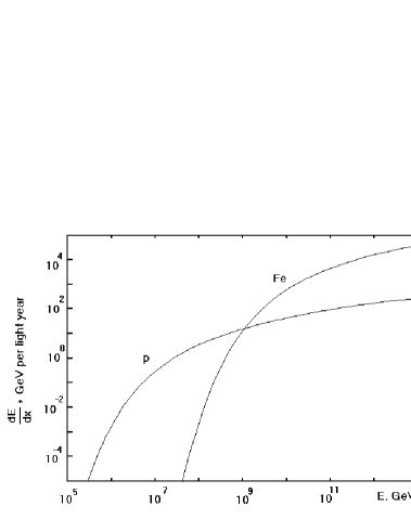
Figure 2: The vacuum polarization energy losses of protons and iron nuclei propagating in the extragalactic space as function of the energy.

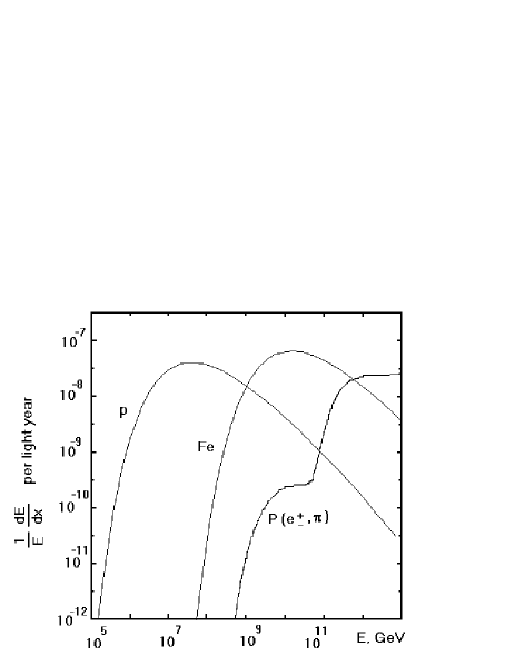
Figure 3: The relative vacuum polarization energy losses of protons and iron nuclei propagating in the extragalactic space as function of the energy. On the right the similar value for photoproduction energy losses (from [2]) is presented for comparison.

References

- [1] M.Nagano and A.A.Wilson, Rev. Mod. Phys. 72 (2000), 689.
- [2] V.Berezinsky, A.Z.Gazizov and S.I.Grigorieva hep-ph/0204357.
- [3] L.Anchordoqui, T.Paul, S. Reucraft, J.Swain hep-ph/0206072.
- [4] S. Lee, Phys. Rev. D, 58 (1998), 043004.
- [5] F.W.Stecker, hep-ph/0101072
- [6] K.-H.Kampert et. al., astro-ph/0102266.
- [7] K.Greisen, Phys. Rev. Lett. 16 (1966), 748.
- [8] G.T. Zatsepin and V.A.Kuzmin, JETP Lett. 4 (1966), 78.
- [9] J. Schwinger, Phys. Rev. 75 (1949), 1912; 82 (1951), 664.
- [10] V.B.Berestetskii, E.M.Lifshitz, L.P.Pitaevskii, Quantum Electrodynamics, Pergamon, Oxford, 1982.
- [11] E.S. Fradkin, D.M. Gitman and Sh. M. Shvartsman. Quantum Electrodynamics with Unstable Vacuum, Springer 1991.
- [12] L.D.Landau, E.M.Lifshitz, Electrodynamics of Continuous Media, Pergamon, New York, 1984.
- [13] V.M.Agranovich and V.L.Ginzburg, Crystal Optics with Spatial Dispersion, and Excitons, 2nd ed., Springer-Verlag, Berlin - New York (1984).
- [14] V.N.Baier, V.N.Katkov, Phys.Lett. A 216 (2001), 299.
- [15] V.A.Maisheev, Zh. Eksp. Teor. Fiz. 112 (1997) 2016 [in Russian]; JETP 85 (1997) 1102
- [16] V.A.Maisheev, Nucl. Inst. and Meth. B 168 (2000), 11.
- [17] R.J.Protheroe and H.Meyer, Phys. Lett. B493 (2000),1; astro-ph/0005349.
- [18] G.Barton, Phys. Lett. B 237 (1990), 559.
- [19] J.I.LaTorre, P.Pascual and R.Tarrach, Nucl. Phys. B437 (1995), 60.
- [20] M.H.Thoma, Europhys. Lett. 52 (2000), 498.
- [21] I.M.Dremin, Pisma v ZhETF 75(2002),199; JETP Lett. 75(2002),4.
- [22] D.H.Perkins, Introduction to high energy physics, Addison - Wesley Com, Inc., 1987.
- [23] T.H. Burnett et. al., Astrophys. J. 349 (1990), L25.
- [24] K.Bernlohr, et. al., Astropat. Phys. 8,(1998), 253.