Nonlinear Behavior of Quarkonium Formation and Deconfinement Signals

Abstract

We anticipate new features of quarkonium production in heavy ion collisions at RHIC and LHC energies which differ from a straightforward extrapolation of results at CERN SPS energy. General arguments indicate that one may expect quarkonium formation rates to increase more rapidly with energy and centrality than the production rate of the heavy quarks which they contain. This is due to new formation mechanisms in which independently-produced quarks and antiquarks form a bound quarkonium state. This mechanism will depend quadratically on the total number of initially-produced heavy quark pairs, and becomes numerically significant only at RHIC and LHC energy. When viewed as a signal of color deconfinement, a transition from suppression to enhancement may be observed. Explicit model calculations are presented, in which one can follow striking variations of final quarkonium production within a range of parameter space.

1 Introduction

The production of heavy quarkonium states in high energy hadronic interactions proceeds through creation of the corresponding flavor heavy quark-antiquark pair. Given the heavy quark mass to provide a perturbative scale, one can employ a perturbative QCD calculation for this initial process Altarelli (2002). The spectrum of heavy quarkonium states can be described by essentially non-relativistic heavy quarks interacting via a static potential. Phenomenological extraction of the potential leads to a linear rise at large separation, which provides the observed quark confinement. This potential can also be directly calculated via lattice methods Karsch (2002), and confirms these general properties. These lattice methods can also be utilized for QCD at finite temperature, which reveals that at sufficiently high T the QCD spectrum will change from confined hadrons to colored degrees of freedom. The corresponding heavy quark static potential in this case shows a decrease in the long range part, and disappears above the deconfinement temperature. The goal of high energy heavy ion collision experiments is to create a region of space-time within which these finite temperature predictions can be tested.

A signature of color deconfinement which utilizes heavy quarkonium production rates was proposed more than 15 years ago Matsui and Satz (1986). One invokes the argument that in the deconfined region where the color-confining force has disappeared, a heavy quark and antiquark cannot form a quarkonium bound state, and they may diffuse away from each other to separations larger than typical hadronic dimensions. As the system cools and the confining potential reappears, these heavy quarks will not be able to “find” each other and form heavy quarkonium. They will then bind with quarks which are close by to them at hadronization. Since these quarks are predominantly the lighter u, d, and s flavors, they will most likely form a final hadronic state with “open” heavy flavor. The result will be a decreased population of heavy quarkonium relative to those which would have formed if a region of deconfinement had not been present. This scenario as applied to the charm sector is known as $J/\psi$ suppression. There are now extensive data on $J/\psi$ production using nuclear targets and beams. Results from the NA50 experiment at the CERN SPS reveal an “anomalous” suppression, prompting claims that this effect could be the expected signature of deconfinement M. C. Abreu (2000). Measurements at higher energies of RHIC, and eventually at the heavy ion runs at LHC, should be able to provide enough information to either support or refute these claims. Straightforward extension of the deconfinement scenarios to these higher energies anticipate that $J/\psi$ suppression would be virtually complete at all centralities Vogt (1999).

The purpose of this work is to point out that there will be another consequence of the increased beam energy for the suppression scenario. This is because one expects that multiple pairs of charm-anticharm quarks will be produced in the initial partonic stage of the collision. Perturbative QCD estimates predict about 10 charm pairs at RHIC energy, and several hundred pairs at LHC McGaughey et al. (1995). This situation provides a “loophole” in the Matsui-Satz argument, since there will be many more heavy quarks in the interaction region with which to combine. In order for this to happen, however, one must invoke a physical situation in which quarkonium states can be formed from all combinations of the heavy quark pairs. If this is possible, then the rate of quarkonium formation from $N$ initially-produced quark-antiquark pairs would initially be proportional to $N^{2}$. If the total number of quarkonium states remains a small fraction of the total number of pairs, then the final population will retain this quadratic dependence. Although still small compared with $N$, this number can be much larger than the “ordinary” expectations which are linear in $N$.

In the next section, we go through the pQCD methods and results which lead to the large $N$-values at high energy. The variation of these quantities with centrality is also explored. The following section presents generic arguments for the properties of quarkonium formation in any physical situation for which the quadratic process is allowed. The last two sections present results specific to two physical models which share some of these properties.

2 Heavy Quark Production in A-A Collisions

The calculation of heavy quark production by hadrons is based on perturbative QCD processes at the parton level. The perturbative approach requires a large scale to justify the expansion in powers of $\alpha_{s}$, which is provided by the heavy quark mass. One then uses hadronic structure functions measured in other reactions (e.g. Deep Inelastic Scattering and Drell-Yan) plus factorization to calculate the hadronic cross section. The general expression is of the form

$$\sigma(s,m_{Q},\mu_{F},\mu_{R})=\sum_{i,j}\int dx_{1}\int dx_{2}F_{i}(x_{1},\mu_{F})F_{j}(x_{2},\mu_{F}){\hat{\sigma}}_{ij}(\hat{s},m_{Q},\mu_{R})$$ (1)

where $i$ and $j$ label the initial state partons, F(x,$\mu_{F}$) are the structure functions, evaluated at a factorization scale $\mu_{F}$, and ${\hat{\sigma}}_{ij}$ are the partonic cross sections for producing a heavy quark-antiquark pair, which depend on the partonic process subenergy $\hat{s}=x_{1}x_{2}s$, the heavy quark mass $m_{Q}$ and the renormalization scale $\mu_{R}$.

The partonic cross sections have been calculated Nason et al. (1988),Mangano et al. (1993),Frixone et al. (1994) to lowest order (LO), in which quark-antiquark annihilation and gluon-gluon fusion and annihilation into $Q\bar{Q}$ contribute to order ${\alpha_{s}}^{2}(\mu_{R})$, and also in next to leading order (NLO), where real gluons emitted in the final states of the LO processes, plus processes involving quark or antiquark plus gluon in the initial state, plus virtual loop corrections all contribute to order ${\alpha_{s}}^{3}(\mu_{R})$. There is additional dependence on $\mu_{R}$ in NLO, in the form of terms proportional to $ln({\mu_{R}^{2}}/{m_{Q}^{2}}).$ In practice one usually takes $\mu_{R}=\mu_{F}\equiv\mu$, but in general they are independent parameters of the calculation, along with $m_{Q}$. In addition, there are several sets of parton distribution functions which can be utilized. In order to constrain these parameters, a comprehensive comparison with existing charm production data in N-N and $\pi$-N reactions was undertaken McGaughey et al. (1995). For a recent update of this procedure, see Reference Vogt (2002).

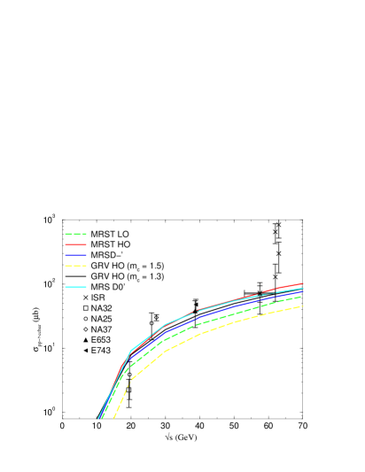
Figure 1: pQCD calculated cross section for $pp\rightarrow c\bar{c}$.

The charm mass $m_{c}$ was allowed to vary between 1.2 and 1.5 GeV, and $\mu$ was varied between $m_{c}$ and 2$m_{c}$. The results for the cross section $pp\rightarrow c\bar{c}$ in the energy interval 10 GeV ¡ $\sqrt{s}$ ¡ 70 GeV are shown in Figure 1.

Results from the original structure function sets MRSD0 and MRSD-^′ are shown, and supplemented by the more recent sets of structure functions MRST HO and GRV HO. The difference in predictions between these sets is in general smaller than the experimental uncertainties, except for the GRV with large $m_{c}$ and the low order set MRST LO, which is only shown for comparison (for consistency one must use the NLO version of the structure functions together with NLO partonic cross sections). However, we must remember that the x-values probed in these calculations are always greater than $m_{c}/\sqrt{s}$, which is large enough such that all structure functions are very well constrained by the DIS and DY data. What one may worry about is the large change in cross section between the LO alone and the total LO + NLO. The ratio of these values (the K-factor) typically varies between 1.5 and 2.5 in this energy region. Thus one might expect that higher order terms in the perturbative expansion (NNLO) might also be as significant as the NLO. In this case, a satisfactory fit to the data would probably require different values of the mass and scale parameters, thus altering the predictions at higher energy.

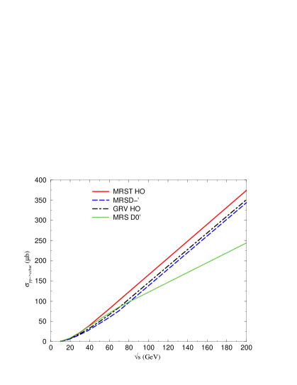
Figure 2: pQCD calculated cross section for $pp\rightarrow c\bar{c}$ extrapolated to RHIC energy.

The extrapolation of these calculations up to RHIC energies is shown in Figure 2. We show only the four structure function sets which agree with the low energy data. One sees that there is some divergence at the highest $\sqrt{s}$ = 200 GeV. However, this plot is on a linear scale, which maximizes the appearance of the differences.

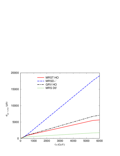
Figure 3: pQCD calculated cross section for $pp\rightarrow c\bar{c}$ extrapolated to LHC energy.

Finally, we show in Figure 3 the extrapolation of these calculations to the LHC heavy ion energy region. The scale is again linear, and there is almost a factor of 10 difference between the old structure function sets. This can be attributed to the low x-values probed at $\sqrt{s}$ = 5500 GeV, down to about $x\approx 3\times 10^{-3}$. The more recent structure functions include DIS data from HERA which is sensitive to these low x-values, and we see that both the MRST and GRV HO sets follow each other much more closely. Note however, that we have not used the complete set of modern structure functions and parameter space values which fit the low energy data. The calculations in Reference Vogt (2002) which do include all of these possibilities predict a range which differs by a factor of 2.3 between highest and lowest values.

We now use these cross sections to predict the number of heavy quark pairs which will be produced in heavy ion collisions. In the simplest case when we assume that the heavy ion collision is just an incoherent superposition of N-N collisions (no shadowing corrections), we only need calculate the integrated N-N luminosity in a single A-A collision. For a central collision between identical nuclei, geometry tells us this should be of the form $A^{2}/\pi R_{A}^{2}\propto A^{4\over 3}$.

For a more general calculation, one needs a parameterization of the nuclear density $\rho_{A}(\vec{s},z)$, where z is the coordinate along the beam direction and $\vec{s}$ is the 2-dimensional position vector in the transverse plane. Then one can calculate a nuclear thickness function

$$T_{A}(\vec{s})=\int dz\,\rho_{A}(\vec{s},z)$$ (2)

which is normalized to the total nuclear number

$$\int d^{2}\,\vec{s}\>T_{A}(\vec{s})=A.$$ (3)

Then consider a collision of two nuclei which are incident along paths parallel to the z-axis separated in the transverse plane by a vector $\vec{b}$ (the magnitude of $\vec{b}$ is the impact parameter b). The integrated N-N luminosity is then just the product of the two nuclear thickness functions integrated over each overlap point in the transverse plane. This is called the nuclear overlap function:

$$\int d^{2}\,\vec{s}\;T_{A}(\vec{s})\,T_{B}(\vec{b}-\vec{s})\equiv T_{AB}(b)$$ (4)

which by axial symmetry can only depend on the impact parameter b.

Calculations using standard nuclear density profiles produce a typical value for heavy ion (e.g. Pb-Pb or Au-Au) of $T_{AA}(b=0)\approx 30mb^{-1}.$ This leads to the estimates of $N_{c\bar{c}}$ for central collisions at the various experimental facilities. Taking average values for the open charm cross section calculations, we obtain $N_{c\bar{c}}$(b=0) = 0.2 (SPS), 10 (RHIC200), and 200 (LHC). The energy dependence and variation with structure function set are shown in Figures 4 and 5.

The first RHIC measurement of open charm has been reported at this institute Zajc (2002),K. Adcox et. al. (2002). From observation of high-$p_{T}$ electrons by the PHENIX Collaboration from the 130 GeV run, an equivalent value of the p-p open charm cross section can be extracted. For central collisions, the reported value is $\sigma(pp\rightarrow c\bar{c})=380\pm 200\mu b$. Although the uncertainties are still quite large, we can already draw some conclusions and make some interesting speculations.

The corresponding $N_{c\bar{c}}$ values for b = 0 collisions are overlayed on Figure 4 and shown in Figure 6. One sees that the magnitude of the calculated values are consistent with the measurement within errors. However, the central value is well above the calculated values, even exceeding the nominal prediction at the higher 200 GeV energy. A simple extrapolation of this central point to $\sqrt{s}$ = 200 GeV would imply $N_{c\bar{c}}$ between 15 and 20. This is substantially above the nominal estimate of 10, and could enhance the expected nonlinear effects for $J/\psi$ formation. This situation is somewhat surprising, since these values are extracted just from nuclear geometry and calculations using structure functions of nucleons. One might expect that there will be a depletion of gluons in a heavy nucleus relative to free nucleons, similar to the shadowing of quark structure functions observed for DIS with nuclear targets Eskola et al. (1999). These speculations, of course, are only relevant assuming the eventual uncertainties of the measured value will converge toward the current central value.

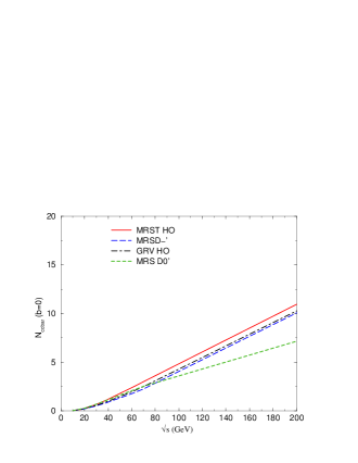
Figure 4: Energy dependence of central $N_{c\bar{c}}$ in RHIC region.

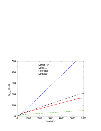
Figure 5: Energy dependence of central $N_{c\bar{c}}$ in LHC region.

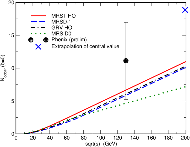
Figure 6: Comparison of PHENIX measurement with pQCD calculations of central $N_{c\bar{c}}$.

We can also use the overlap function $T_{AA}(b)$ to predict the centrality dependence. However, the impact parameter $b$ is not directly measurable. Instead, the number of participant nucleons $N_{p}$ is generally used as a connection between nuclear geometry and experimental measurables. Most experiments measure the transverse energy $E_{T}$ of each event and relate this to centrality. For this, one needs a model for $N_{p}$. One popular choice is the wounded nucleon model Białas et al. (1976), in which every nucleon which undergoes at least one inelastic collision is called “wounded” and is counted as a participant nucleon. The utility is reinforced by the experimental observation that $N_{p}$ and $E_{T}$ are linearly-related over quite a wide range in centrality Margetis et al., NA49 Collaboration (1995). We show in Figure 7 the calculated dependence of $N_{w}$ on impact parameter, using standard nuclear density profiles and an inelastic N-N cross section of 50 mb. A similar behavior to that of the nuclear overlap function $T_{AA}$ is evident. Also shown for future reference (dotted line) is the wounded nucleon density in impact parameter space (evaluated at the center of the overlap area). We can then recast the centrality dependence of $T_{AA}$(b) in terms of the participant (or in this case wounded) nucleon number. This is shown in Figure 8.

One sees that there is a power law dependence, $T_{AA}\propto N_{w}^{4/3}$. This relationship could have been anticipated from the general arguments concerning equivalent N-N integrated luminosity, but it is pleasing to verify in an explicit model.

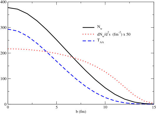
Figure 7: Wounded nucleon and nuclear overlap dependence on impact parameter.

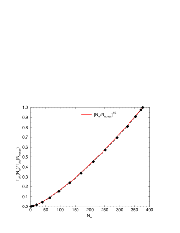
Figure 8: Centrality dependence of $T_{AA}$ in terms of $N_{w}$.

Finally, one can plot the predictions for $N_{c\bar{c}}$ as a function of centrality, using participant nucleon number $N_{p}$ as a label. This is shown in Figure 9 for SPS, RHIC200, and LHC energies. The multiple points in each curve come from using several structure function sets. The decrease with centrality just follows the power law behavior of $T_{AA}$, and one sees that at sufficiently peripheral collisions the average number of charm pairs produced will decrease below unity for all energies considered. This behavior will be a very useful constraint on the models to be considered.

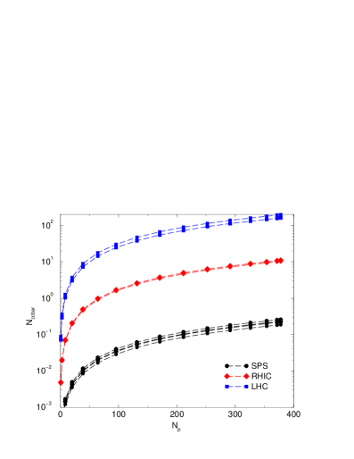
Figure 9: Centrality dependence of $N_{c\bar{c}}$.

3 Quarkonium Formation from Uncorrelated Pairs

As shown in the previous section for heavy ion collision energies at RHIC and LHC, the initial number of heavy quark pairs produced in each collision will be qualitatively different than the number produced at SPS energies. To be specific, let us consider charm quarks and the subsequent production/formation of $J/\psi$. Typically, the number of charm quark pairs is expected to be of the order of ten at RHIC and several hundred at LHC in the most central collisions McGaughey et al. (1995). Let us attempt to extract features of $J/\psi$ formation from the initially-produced charm quarks which are independent of detailed dynamics Thews (2002).

We consider scenarios in which the formation of $J/\psi$ is allowed to proceed through any combination of one of the $N_{c}$ charm quarks with one of the $N_{\bar{c}}$ anticharm quarks which result from the initial production of $N_{c\bar{c}}$ pairs in a central heavy ion collision. This of course would be expected to be valid in the case that a space-time region of color deconfinement is present, but is not necessarily limited to this possibility. For a given charm quark, one expects then that the probability $\cal{P}$ to form a $J/\psi$ is proportional to the number of available anticharm quarks relative to the number of light antiquarks,

$${\cal{P}}\propto N_{\bar{c}}/N_{\bar{u},\bar{d},\bar{s}}\approx N_{c\bar{c}}/N_{ch}.$$ (5)

In the second step we have replaced the number of available anticharm quarks by the total number of pairs initially produced, which assumes that the total number of bound states formed remains a small fraction of the total. Also, we normalize the number of light antiquarks by the number of produced charged hadrons. Since this probability is generally very small, one can simply multiply by the total number of charm quarks $N_{c}$ to obtain the number of $J/\psi$ expected in a given event.

$$N_{J/\psi}\propto{N_{c\bar{c}}}^{2}/N_{ch},$$ (6)

where the use of the initial values $N_{c\bar{c}}=N_{c}=N_{\bar{c}}$ is again justified by the relatively small number of bound states formed. For an ensemble of events, the average number of $J/\psi$ per event is calculated from the average value of initial charm $<N_{c\bar{c}}>$, and we neglect fluctuations in $N_{ch}$.

$$<J/\psi>=\lambda(<N_{c\bar{c}}>+1)<N_{c\bar{c}}>/N_{ch},$$ (7)

where we place all dynamical dependence in the parameter $\lambda$.

One can extend this formula to the case where $J/\psi$ formation is effective not over the entire rapidity range $Y_{total}$, but only if the quark and antiquark are within the same rapidity interval $\Delta y$. There is a significant simplification if the rapidity dependence of the charm quark pairs and the charged hadrons (or equivalently the light antiquarks) are the same. In this case the entire effect is just the replacement $<N_{c\bar{c}}>+1\rightarrow<N_{c\bar{c}}>+Y_{total}/\Delta y$. However, one must remember that the prefactor $\lambda$ will in general contain some dependence on the size of the rapidity interval.

The essential property of this result is that the growth with energy of the term quadratic in total charm McGaughey et al. (1995) is expected to be much stronger than the growth of total particle production in heavy ion collisions Wang and Gyulassy (2001). $J/\psi$ production without this quadratic mechanism is typically some small energy-independent fraction of total initial charm production Gavai et al. (1995), so that we can expect the quadratic formation to become dominant at high energy.

We show numerical results in Table 1 for these quantities with a prefactor $\lambda$ of unity. Estimates for the charm and particle numbers are very approximate, but serve to show the anticipated trend with energy. At SPS, this formation mechanism is most probably insignificant. At RHIC it is comparable with “normal” formation, while at LHC one might expect it to be dominant. Of course, the exact result will depend on the details of the physics which controls the formation.

Table 1: Comparison of $J/\psi$ formation variation with energy

	$SPS$	$RHIC$	$LHC$
$\sqrt{s}$ (GeV)	18	200	5500
$<N_{c\bar{c}}>$	0.2	10	200
$N_{ch}$	1350	3250	16500
$<N_{J/\psi}>$	0.00018	0.034	2.4
$N_{J/\psi}^{initial}$	0.0012	0.06	1.2

We can also estimate the centrality dependence of $J/\psi$ production from Equation 7. The number of charm quark pairs should obey

$$N_{c\bar{c}}\propto{N_{p}}^{4/3}$$ (8)

from the properties of the nuclear overlap function. The number of hadrons produced generally scales with the number of participants,

$$N_{ch}\propto{N_{p}}^{\alpha},$$ (9)

where one has measured values $\alpha=1.07\pm 0.04$ at SPS M.M.Agarwal et al. (WA98 Collaboration) and $\alpha=1.13\pm 0.05$ at RHIC-130 K. Adcox etal Phenix Collaboration (2001). At LHC, one might anticipate that hadron production would become dominated by QCD minijets Wang and Gyulassy (2001), so that $\alpha\approx 4/3$. However, a comparison of RHIC results at 130 and 200 GeV does not indicate a dramatic effect in this energy range. B. B. Back (2002),I. G. Bearden (2001)

Given these values, one can predict

$$N_{J/\psi}\propto{N_{p}}^{\beta={8\over 3}-\alpha}$$ (10)

for collisions in which $<N_{c\bar{c}}>\;\;\gg 1$, and

$$N_{J/\psi}\propto{N_{p}}^{\beta={4\over 3}-\alpha}$$ (11)

for collisions in which $<N_{c\bar{c}}>\;\;\ll 1$.

One can make an indirect check of the prediction at SPS energy, utilizing the NA50 data M. C. Abreu (2000) on ($J/\psi$)/DY as a function of transverse energy $E_{T}$. Since there is a linear relationship between $E_{T}$ and $N_{p}$ over almost the entire measured range, we can just multiply the measured ratios at each $E_{T}$ by the expected centrality dependence of the Drell-Yan process, ${E_{T}}^{4/3}$. This is shown in Figure 10.

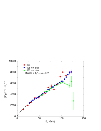
Figure 10: Centrality dependence of $J/\psi$ inferred from measured ratio $J/\psi$/Drell-Yan by NA50 at SPS.

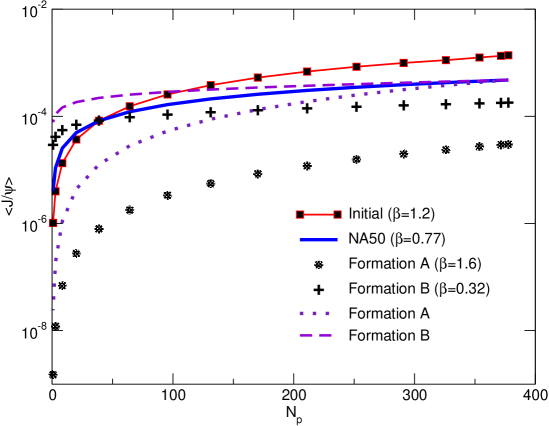
Figure 11: Generic $J/\psi$ production at SPS

A power-law fit to the resulting points yields an exponent $\beta\approx 0.77$. This value is significantly higher than one would predict from the generic arguments above, since at SPS with $<N_{c\bar{c}}>\,\ll 1$, $\beta\approx{4\over 3}-\alpha\approx 0.26$. Figure 11 illustrates this feature.

As a reference, the expected centrality dependence for initial $J/\psi$ production is shown, which includes the hard production process followed by normal nuclear absorption. The parameterization of the absorption cross section is taken from Kharzeev et al. (1997), which leads to an effective power law exponent $\beta\approx 1.2$ The solid line shows the centrality dependence implied by the NA50 data described above, and is normalized such that it coincides with the initial production value for sufficiently peripheral collisions. The predictions of the generic quadratic formation formula are shown by the stars (labeled A). Of course, the initial charm production at SPS energies is certainly small enough such that the linear dependence is dominant. This effect is shown by the plus symbols (labeled B), which include both the quadratic and linear terms. A single power law fit to this composite curve yields $\beta$ = 0.32, again indicative that the linear term with its own $\beta$ = 0.26 is dominant. Also shown by the dotted and dashed lines are these same curves, but normalized for central collisions to coincide with the “NA50” curve for ease of comparison. It is clear that the centrality dependence implied by the NA50 data is not reproduced by the generic expectations. In this respect it is fortunate that the expected magnitude of $J/\psi$ formation implied by the generic arguments is likely to be insignificant at SPS energies.

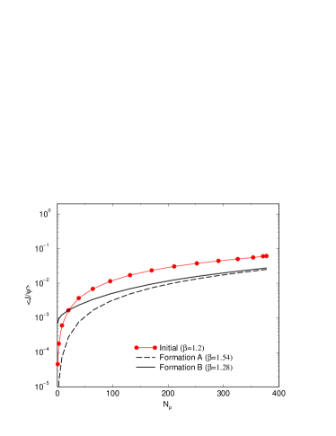
Figure 12: Generic $J/\psi$ production at RHIC

The corresponding results at RHIC energy are shown in Figure 12. Again the generic formation curves use the prefactor $\lambda$ = 1. Here we have used the expected charm yield of 10 pairs per central collision at 200 GeV, but used the measured $\alpha$ value at 130 GeV. At RHIC, one expects to see the quadratic dependence for central collisions (Curve A) gradually convert to linear dependence as appropriate for the small number of $N_{c\bar{c}}$ for peripheral collisions. Curve B shows the combination of linear and quadratic components, which is fit by a single power $\beta$ = 1.28 (indicates the quadratic component dominates over most of the centrality range). Figure 13 contains the same calculations at LHC energy. Here the purely quadratic formula (B) is dominant over the entire centrality region, since the number of charm pairs for central collisions is so large ($\approx 200$). We have assumed at LHC energy that the particle production centrality dependence has increased as appropriate for total domination by minijets. If this is not correct, the $\beta$ values will be even higher but the dominance of the quadratic term will remain.

We compile in Figure 14 the expected centrality dependence for all energies considered. The absolute magnitudes correspond to the prefactor $\lambda$ = 1. Also shown is the dependence implied by the NA50 data, which is normalized to coincide with the generic SPS curve for the most central point. Certainly the centrality dependence at RHIC and LHC will be crucial for the interpretation of any enhanced $J/\psi$ production.

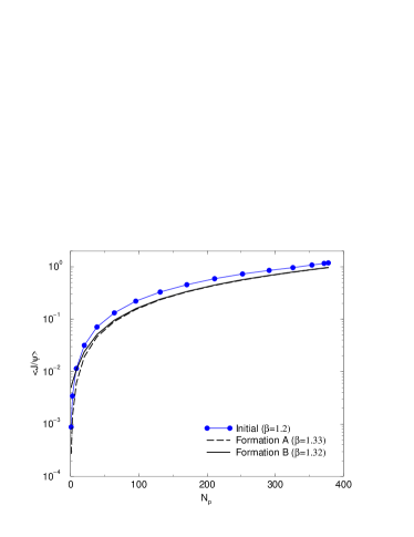
Figure 13: Generic $J/\psi$ production at LHC

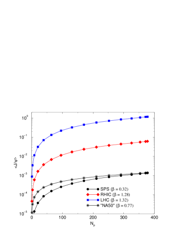
Figure 14: Centrality dependence of generic $J/\psi$ production with dynamical factor $\lambda$ = 1.

4 STATISTICAL HADRONIZATION MODEL

This model is motivated by the success of attempts to explain the relative abundances of light hadrons produced in high energy interactions in terms of the predictions of a hadron gas in chemical and thermal equilibrium Braun-Munzinger et al. (2001). Such fits, however, are not able to describe the abundances of hadrons containing charm quarks. This can be understood in terms of the long time scales required to approach chemical equilibrium for heavy quarks. However, it is expected that for high energy heavy ion collisions the initial production of charm quark pairs exceeds the number expected at chemical equilibrium as determined by the light hadron abundances. As an illustration, we show in Figure 15 the density of charm quarks in equilibrium over a range of temperatures. This is compared with the charm quark density which results from distributing the initially-produced charm quark pairs over the volume of a deconfined region. Each line in the figure corresponds to a different initial temperature. The decrease in the density as temperature decreases is due to the expansion of the deconfined region. (We use nominal RHIC conditions for central collisions, $N_{c\bar{c}}$ = 10, initial volume $V_{o}=\pi R^{2}\tau_{o}$ with $\tau_{o}$ = 1 fm, and isentropic longitudinal expansion, $VT^{3}$ = constant.) One sees that at temperatures below typical deconfinement transitions, the initial charm densities all exceed that expected for thermal equilibrium. (This will always happen at some finite T, since the decrease of equilibrium density is exponential while the initial densities only decrease due to power law volume expansion.)

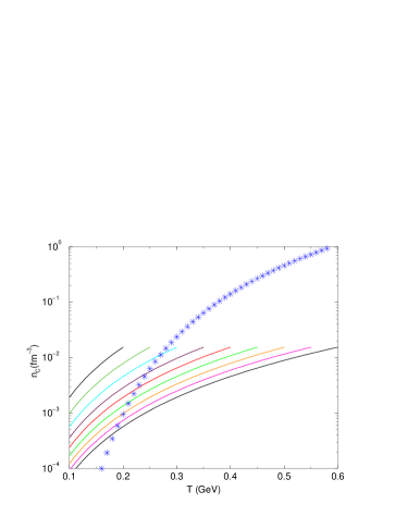
Figure 15: Charm quark density.

The statistical hadronization model assumes that at hadronization these charm quarks are distributed into hadrons according to chemical and thermal equilibrium, but adjusted by a factor $\gamma_{c}$ which accounts for oversaturation of charm density. One power of this factor multiplies a given thermal hadron population for each charm or anticharm quark contained in the hadron. Thus the relative abundance of $J/\psi$ to that of D mesons, for example, will be enhanced in this model. The enhancement factor is determined by conservation of charm, again using the time scale argument to justify neglecting pair production or annihilation before hadronization.

$$N_{c\bar{c}}={1\over 2}\gamma_{c}N_{open}+{\gamma_{c}}^{2}N_{hidden},$$ (12)

where $N_{open}$ is the number of hadrons containing one charm or anticharm quark and $N_{hidden}$ is the number of hadrons containing a charm-anticharm pair. (The contribution of multiply-charmed baryons or antibaryons are generally neglected since their large mass leads to very small thermal densities.) Note that the actual particle numbers, not just the densities, are required in this approach. Thus the volume of the thermal system is an additional parameter which must be included.

For most applications, $N_{hidden}$ in Equation 12 can be neglected compared with $N_{open}$ due to the hadronic mass differences. Thus the charm enhancement factor is simply

$$\gamma_{c}={2N_{c\bar{c}}\over N_{open}}.$$ (13)

This is easily seen to predict a quadratic dependence of the population of hidden charm hadrons. Using the thermal densities allows one to calculate the prefactor $\lambda$ from the previous section.

$$N_{J/\psi}={\gamma_{c}}^{2}{N_{J/\psi}}^{thermal}$$ (14)

It is important to note at this time that $N_{J/\psi}^{thermal}$ includes the thermal population of all hidden charm states which decay into the observed $J/\psi$. Since all of the individual terms are multiplied by the same charm factor $\gamma_{c}^{2}$, the statistical hadronization model predicts that all ratios of various hidden charm state populations are identical to those predicted by the thermal densities alone. It was first noted in Reference Sorge et al. (1997) that the measured ratio ${\Psi^{\prime}/\Psi}$ for heavy ion interactions at SPS was quite close to that expected in thermal equilibrium at temperature close to the deconfinement transition for sufficiently central collisions.

We replace the one remaining factor of system volume by the ratio of charged particle number to density to compare with the generic expectations in Equation 6.

$$N_{J/\psi}=4{n_{ch}n_{J/\psi}\over{n_{open}}^{2}}{N_{c\bar{c}}^{2}\over N_{ch}}$$ (15)

This is the result contained in the initial formulation of the statistical hadronization model Braun-Munzinger and Stachel (2000), where the goal was to compare with results of the NA50 experiment on $J/\psi$ production. It was soon realized Braun-Munzinger and Stachel (2001), Gorenstein et al. (2001) that for such an application, an important correction must be applied to Equation 12. We have tacitly assumed up to now that the thermal particle numbers $N_{open}$ and $N_{hidden}$ have been calculated in the grand canonical formalism, and that they are large enough such that charm conservation is satisfied by the average values with fluctuations suppressed by these large particle numbers. However, one knows that at SPS energies the average thermal charm numbers per collision are much less than unity for all collision centrality. Even at RHIC and LHC, sufficiently non-central events will always involve small particle numbers. In these cases, one cannot satisfy exact charm conservation on the average, and one must utilize the canonical formalism to calculate the thermal particle numbers. This is obvious in the limiting case where each collision produces either one or zero charm quark pairs, and they can go only into either one hidden charm hadron or one charm and one anticharm hadron Redlich et al. (2002).

There is a simple correction factor which can be applied to calculate the canonical particle number $N_{can}$ from the grand canonical particle number $N_{gc}$ for a thermal system in which the conserved quantity (charm in this case) population in baryons can be neglected (justified by large masses).

$$N_{can}=N_{gc}{{I_{1}(N_{gc})}\over{I_{0}(N_{gc})}}.$$ (16)

which just involves the modified Bessel functions $I_{n}$ Cleymans et al. (1991). One uses this expression with $N_{gc}=\gamma_{c}N_{open}$ to revise Equation 12. Note that there is no canonical correction for $N_{hidden}$, which has zero total charm.

$$N_{c\bar{c}}={1\over 2}\gamma_{c}N_{open}{{I_{1}(\gamma_{c}N_{open})}\over{I_{0}(\gamma_{c}N_{open})}}+{\gamma_{c}}^{2}N_{hidden},$$ (17)

In the limit of large $N_{gc}$, the ratio of Bessel functions approaches unity, and one recovers the grand canonical result. In the opposite limit when $N_{gc}$ approaches zero, the ratio of Bessel functions goes to ${1\over 2}N_{gc}$, and the solution for the charm enhancement factor is

$$\gamma_{c}\rightarrow{2\sqrt{N_{c\bar{c}}}\over N_{open}}.$$ (18)

The net effect in this limit is then just to change the dependence on $N_{c\bar{c}}$ in Equation 15 from quadratic to linear.

In general, a solution for $\gamma_{c}$ as a function of $N_{c\bar{c}}$ must be obtained numerically. Such a solution is shown in Figure 16, using some specific values of $N_{open}$ and $N_{hidden}$ for charm. One sees the quadratic behavior in the large $N_{c\bar{c}}$ limit and also the linear behavior in the small $N_{c\bar{c}}$ limit. Also shown on this plot is a curve which follows the exact solution for Equation 12, but with $N_{c\bar{c}}$ replaced by $(N_{c\bar{c}}(N_{c\bar{c}}+1))^{1\over 2}$.

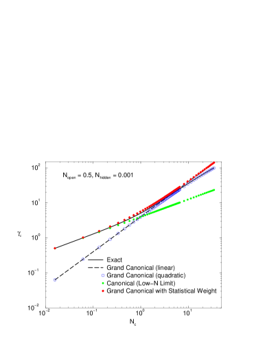
Figure 16: Relation between charm enhancement factor and total number of charm quarks for statistical hadronization model.

It is interesting to note that this replacement allows the grand canonical solutions to incorporate the behavior of the canonical corrections to an impressive degree of accuracy. It appears that the ad hoc substitution above could be motivated by an averaging procedure for $N_{c\bar{c}}^{2}$, which has been noted previously for the two limiting cases Gorenstein et al. (2001). However, apparent general validity of this procedure requires further study, and may involve the properties of the kinetic equations which describe the approach to equilibrium.

This formalism was originally applied to the NA50 measurement of $J/\psi$ production in fixed-target heavy ion collisions at the CERN SPS. There remain uncertainties in the absolute magnitude of $J/\psi$ yields, which has lead to different approaches in the literature. One method is to assume knowledge of $N_{c\bar{c}}$ from measurements in N-N interactions scaled up to heavy ion interactions as appropriate for a point-like process, Then the $J/\psi$ can be predicted, including the centrality dependence. The other approach takes $N_{c\bar{c}}$ as a parameter to be fixed by the measured $J/\psi$ yields. In both cases Braun-Munzinger and Stachel (2001), Gorenstein et al. (2001), a common conclusion appears to emerge. One must require that the magnitude of charm production must be a factor of 3-5 greater than that inferred from N-N interactions, and the centrality dependence must increase much more rapidly than the ${N_{p}}^{4\over 3}$ expected for the pQCD production process. This conclusion may be related to the observation of an excess of dileptons in the intermediate mass region by NA50 M. C. Abreu (2002) for which one source could be enhanced charm production. This situation underscores the need for separate measurements of both total charm and charmonium production in order to test the production mechanisms. Experiment NA60 is expected to provide this information at SPS.

Next we look at applications of the statistical hadronization model at RHIC and LHC. Since the general properties of this model obey the generic expectations of the previous section, we can utilize the generic expectations for centrality dependence. The overall magnitudes are determined by the thermal parameters (including volume), and are generally taken from existing thermal fits to light hadron species. We choose to show the ratio $<J/\psi>$/charm, which is less sensitive to the normalization of total charm production the absolute number of $J/\psi$.

Figure 17 shows several applications for RHIC conditions.

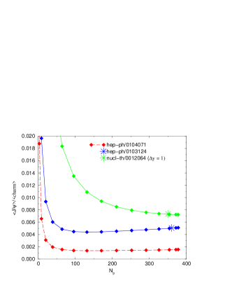
Figure 17: Ratio $<J/\psi>$ over initial charm at RHIC for several applications of the statistical hadronization model.

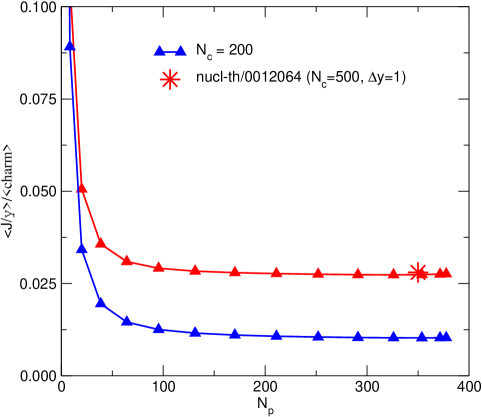
Figure 18: Ratio $<J/\psi>$ over initial charm at LHC for two applications of the statistical hadronization model.

The centrality dependence is modeled by the number of nucleon participants, and one sees the change in shape due to the transition between canonical and grand canonical formalism. The absolute magnitudes of $<J/\psi>$/charm are comparable with the initial production estimates of a fraction of a percent, indicating that this process may overwhelm suppression for central collisions at RHIC. The lowest curve is the calculation of Reference Gorenstein et al. (2001), which includes the centrality dependence. The next higher is from Reference Grandchamp and Rapp (2001) which only included the most central collision point. The same is true for the highest curve from Reference Braun-Munzinger and Stachel (2001), which uses rapidity intervals of width $\Delta y$ = 1 as a requirement for the quarks to form the $J/\psi$. I have completed the calculation of implied centrality dependence for these two calculations. Note that the highest curve exhibits a stronger rise for lower centrality events than the others, since with total charm quark numbers limited by one unit of rapidity, the region which receives a substantial canonical ensemble correction extends further toward very central events.

Corresponding information is shown in Figure 18 for LHC energy. Here we have completed the centrality dependence for one case considered in the literature Braun-Munzinger and Stachel (2001), and contrast it with the generic calculation with no constraint on rapidity interval. Typical magnitudes are factors of 3-5 above the corresponding predictions for RHIC, indicating a strong enhancement of $J/\psi$ formation in the statistical hadronization model.

5 KINETIC FORMATION MODEL

In this model Thews et al. (2001),Thews and Rafelski (2002) , we investigate the possibility to form $J/\psi$ directly in a deconfined medium. The formation will take advantage of the mobility of initially-produced charm quarks in a spatial region of deconfinement. Then one expects that interactions can occur between a charm quark which was produced along with its anticharm partner in one of the initial nucleon-nucleon collisions, and an anticharm quark which was produced with its own charm partner in an entirely different initial nucleon-nucleon collision. Thus all combinations of a charm plus anticharm quarks in the initial $N_{c\bar{c}}$ are allowed to participate in the formation of charmonium states. Of course, there is an upper limit of $N_{c\bar{c}}$ itself on the total number of charmonium states which can be formed, but in practice this limit will never be approached. Since the rates of formation are quadratic in the number of unbound charm pairs, one anticipates that the final charmonium population will be approximately quadratic in the initial value $N_{c\bar{c}}$. In this respect, it then fits in with the generic expectations previously derived based on probabilities of quark number combinations. However, the additional dependence of that generic expectation on hadron production will come about in an entirely different manner.

For the purposes of this study, we consider a physical picture of deconfinement in which the “standard” quarkonium suppression mechanism is via collisions with free gluons in the deconfined medium Kharzeev and Satz (1994). The dominant formation process, in which a quark and an antiquark in a relative color octet state are captured into a color singlet bound quarkonium state and emit a color octet gluon, is simply the inverse of the the breakup reaction which is responsible for the suppression. It is then an inevitable consequence of this picture of suppression that the corresponding formation process must also take place.

At this point one might ask about the effect of color screening in this picture. One view might be that the most deeply bound quarkonium states can still exist above the deconfinement temperature, and that this formation mechanism (and of course the competing dissociation mechanism) will only exist for temperatures above the deconfinement temperature (since we require mobile heavy quarks) but still below some critical temperature $T_{screen}$ which defines the point at which the quarkonium state can no longer exist. In this case the new formation mechanism will just modify the dissociation effectiveness, although in the case of very large numbers of quark pairs this modification will be sufficient to actually change the sign of the effect. In this study we advocate an alternate viewpoint. In this viewpoint, both the color screening mechanism and the gluon dissociation reaction are the same physical phenomenon, but manifest themselves in two different limiting cases. In the limit of very large time scales, the screening view is appropriate, since it assumes that the heavy quarks are subject to a static potential which determines the bound state spectrum. In the limit of very small time scales, the quarkonium states cannot be expected to follow the fluctuations of the color fields due to the light quarks and gluons, and it is assumed that a collisional description will be appropriate. Work is underway Sucipto and Thews (2002) on quantifying these arguments. Initial results indicate that the time necessary to completely screen away a deeply bound quarkonium state is comparable to estimated lifetimes for a deconfined state in heavy ion collisions.

Given the above assumptions, we consider the dynamics of charm quark pairs and $J/\psi$’s in a region of color deconfinement populated by a thermal density of gluons. The time evolution if the $J/\psi$ population is given by the rate equation

$$\frac{dN_{J/\psi}}{d\tau}=\lambda_{\mathrm{F}}N_{c}\,N_{\bar{c}}[V(\tau)]^{-1}-\lambda_{\mathrm{D}}N_{J/\psi}\,\rho_{g}\,,$$ (19)

with $\rho_{g}$ the number density of gluons, $\tau$ the proper time and $V(\tau)$ the volume of the deconfined spatial region. The reactivities $\lambda_{F,D}$ are the reaction rates $\langle\sigma v_{\mathrm{rel}}\rangle$ averaged over the momentum distribution of the initial participants, i.e. $c$ and $\bar{c}$ for $\lambda_{F}$ and $J/\psi$ and $g$ for $\lambda_{D}$. The gluon density is determined by the equilibrium value in the QGP at each temperature. For simplicity, it is assumed to be spatially homogeneous, as are the charm quark and $J/\psi$ distributions.

We enforce exact charm conservation in solving this equation, but in practice this means that the number of charm quarks $N_{c}$ and anticharm quarks $N_{\bar{c}}$ are always approximately equal to the number of initial pairs $N_{c\bar{c}}$ for the following reasons: (a) Reactions in which charm quark-antiquark pairs annihilate into light quarks or gluons are small since the charm density due to initial charm is less than the thermal equilibrium value over during most of the time; (b) Production of additional charm quark pairs from interactions of light quarks and gluons is negligible during the time of deconfinement Rafelski et al. (1996); (c) Formation of other states in the charmonium spectrum is a small fraction of initial charm (as is the fraction of $J/\psi$ itself); and (d) Disappearance of single charm quarks or antiquarks via formation of open charm mesons is effectively reversed immediately because the time scale for dissociation of these large states with small binding energy is typically less than a fraction of a fermi.

To illustrate this last point and set the relevant time scales, we show in Figure 19 the dissociation rates for thermal gluons on various states of quarkonium, as a function of gluon temperature. The reaction cross section used will be discussed below.

Figure 19: Dissociation rates of various bound states of charm due to interactions with thermal gluons.

The behavior with binding energy and spatial bound state size is evident. Certainly the open charm mesons will have typical dissociation times much less than 1 fm. It is also clear that the heavy quarkonium bound states have dissociation times between 1 and 100 fm for typical QGP temperatures, making this process relevant during the time of deconfinement. Note that the temperature dependence arises from two effects. The initial rapid increase in the low temperature region starts when average gluon energies are able to overcome the dissociation threshold, and the continued rise for large temperature is due to the continuing increase in gluon density.

We allow the system to undergo a longitudinal isentropic expansion, which fixes the time-dependence of the volume V($\tau$) = $V_{o}\tau/\tau_{o}.$ The expansion is taken to be isentropic, $VT^{3}$ = constant, which then provides a generic temperature-time profile.

It is evident that the solution of Equation 19 grows quadratically with initial charm $N_{c\bar{c}}$, as long as the total $J/\psi\ll N_{c\bar{c}}$. In this case we can write an analytic expression

$$N_{J/\psi}(\tau_{f})=\epsilon(\tau_{f})\times[N_{J/\psi}(\tau_{0})+N_{c\bar{c}}^{2}\int_{\tau_{0}}^{\tau_{f}}{\lambda_{\mathrm{F}}\,[V(\tau)\,\epsilon(\tau)]^{-1}\,d\tau}],$$ (20)

where $\tau_{f}$ is the hadronization time determined by the initial temperature ($T_{0}$ is a variable parameter) and final temperature ($T_{f}$ ends the deconfining phase). The function $\epsilon(\tau_{f})=e^{-\int_{\tau_{0}}^{\tau_{f}}{\lambda_{\mathrm{D}}\,\rho_{g}\,d\tau}}$ would be the suppression factor in this scenario if the formation mechanism were neglected. During the remainder of these calculations, we concentrate on solutions in which the initial number of produced $J/\psi$ is zero. Then the additional term due to the new formation mechanism represents the final number of $J/\psi$ which result from a competition between the formation and dissociation reactions during the lifetime of the deconfined region. Note that this number is always positive, since one cannot dissociate more bound states than are formed.

We can then compare this additional term with what is anticipated from the generic considerations summarized in Equation 7. The quadratic factor $N_{c\bar{c}}^{2}$ is present as expected. The normalizing factor of $N_{ch}$ does not appear automatically. (Remember that this factor was obtained in the statistical hadronization model by replacing a factor of system volume $V$ by the ratio of $N_{ch}$ over the thermal charged hadron density.) In the kinetic model result, the additional formation term in Equation 20 also has a volume term present. This volume is present to account for the decreasing charm quark density during expansion. It also has some other essential differences. First, the kinetic model volume is time-dependent, and is integrated over the duration of deconfinement. Second, the transverse area of the volume is determined not just by nuclear geometry, but by the dynamics which determine over which region there will be deconfinement. Finally, the factor $\epsilon(\tau_{f})/\epsilon(\tau)$ due to dissociation processes during deconfinement will play a role. These differences will be seen explicitly when the centrality dependence is considered.

For our quantitative estimates, we utilize a cross section for the dissociation of $J/\psi$ due to collisions with gluons which is based on the operator product expansion Peskin (1979),Bhanot and Peskin (1979):

$$\sigma_{D}(k)={2\pi\over 3}\left({32\over 3}\right)^{2}\left({2\mu\over\epsilon_{o}}\right)^{1/2}{1\over 4\mu^{2}}{(k/\epsilon_{o}-1)^{3/2}\over(k/\epsilon_{o})^{5}},$$ (21)

where $k$ is the gluon momentum, $\epsilon_{o}$ the binding energy, and $\mu$ the reduced mass of the quarkonium system. This form assumes the quarkonium system has a spatial size small compared with the inverse of $\Lambda_{QCD}$, and its bound state spectrum is close to that in a nonrelativistic Coulomb potential. These assumptions are somewhat marginal for the charmonium spectrum, but should be better satisfied for the upsilon states.

The magnitude of the cross section is controlled just by the geometric factor ${4\mu^{2}}$, and its rate of increase in the region just above threshold is due to phase space and the p-wave color dipole interaction. This same cross section is utilized with detailed balance factors to calculate the primary formation rate for the capture of a charm and anticharm quark into the $J/\psi$.

We use parameter values for thermalization time $\tau_{0}$ = 0.5 fm, initial volume $V_{0}=\pi R^{2}\tau_{0}$ with R = 6 fm, deconfinement temperature $T_{f}$ = 150 MeV, and a wide range of initial temperatures 200 MeV $<T_{0}<$ 600 MeV. We begin by showing some results which assume also thermal charm quark momentum distributions, but this will be generalized later.

Shown in Figure 20 is one typical time evolution of $J/\psi$ taken from our numerical solutions. Also shown are the time dependence of the formation and dissociation reactions.

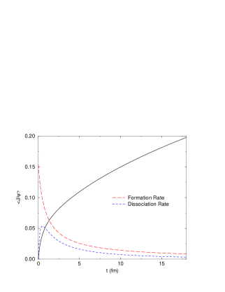
Figure 20: Time dependence of formation and dissociation rates and total $<N_{J/\psi}>$ at RHIC energy.

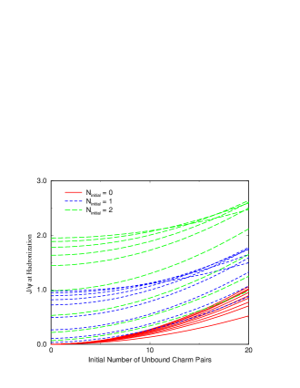
Figure 21: Quadratic dependence of $<J/\psi>$ as a function of total initial charm.

falls due to the decrease in charm quark density with the expanding volume. The dissociation rate starts out at zero since there are no initial $J/\psi$’s, but then jumps up to follow the $J/\psi$ population. This rate also eventually decreases due to the drop in average gluon energy related to the falling temperature. The net number of $J/\psi$ formed continues to increase with time as the formation and dissociation rates both slowly decrease. One might wonder at what point one would reach equilibrium, where the two rates would cancel exactly. The answer is that in this case we have controlled the temperature by external means, and equilibrium is never attained during the lifetime of the deconfinement. If we had assumed a constant temperature and volume, there would of course be an equilibrium point beyond which the $J/\psi$ population would become constant.

Figure 21 shows the final $J/\psi$ population as a function of $N_{c\bar{c}}$ for a range of values which include that expected for central collisions at RHIC.

For these calculations, we also allowed the initial $J/\psi$ number to be nonzero. The solid, short dashed, and dashed lines correspond to $N_{J/\psi}(\tau_{o})$ = 0, 1, and 2, respectively. Variation within these line types is from variation of the initial temperature parameter $T_{o}$, which also controls the volume expansion and lifetime. One sees the expected quadratic dependence on $N_{c\bar{c}}$ for all parameter choices. The solid curves are the quantity of main interest, where the initial $J/\psi$ is zero. At the expected $N_{c\bar{c}}$ = 10, one sees final $J/\psi$ in the range of 0.1 to 0.3 per central collision. This is at or above the number one would expect from 10 initial ccbar pairs in N-N interactions, and suggests that the formation process will be competitive at RHIC energy. The two sets of dashed curves show how the dissociation of the initial population adds to the final number, and the expected temperature dependence of this dissociation.

At this point we digress somewhat to examine the effects of varying some of our parameters or assumptions.

• 

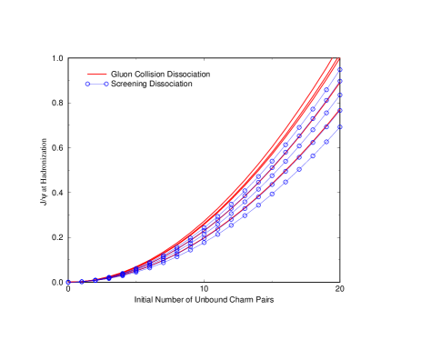
  Figure 22: Comparison of screening and collisional dissociation scenarios.

• In our model of a deconfined region, we have used the vacuum values for masses and binding energy of $J/\psi$, and assumed that the effects of deconfinement are completely included by the dissociation via gluon collisions. For a complementary viewpoint, we have also employed a deconfinement model in which the $J/\psi$ is completely dissociated when temperatures exceed some critical screening value $T_{s}$. Below that temperature, the new formation mechanism will still be able to operate, and we use the same cross sections and kinematics.

  We find that for $T_{s}$ = 280 MeV, the final $J/\psi$ population is approximately unchanged. This behavior is shown in Figure 22. The solid lines are our previous yield curves using gluon collision dissociation for various $T_{o}$, and the circles show the corresponding results with a screening cutoff temperature $T_{s}$ = 280 MeV. One finds that for lower values of $T_{s}$ the formation mechanism produces fewer $J/\psi$, since the most effective formation period is during the initial times when the total volume is small and the corresponding charm quark densities are large. Shown in Figure 23 is the variation of the final yields with $T_{s}$, for various temperature-time profiles. One sees that one could get reductions in formation up to factors of 2 or 3 in this scenario.

• The validity of the cross section used assumes strictly nonrelativistic bound states, which is somewhat marginal for the $J/\psi$. All of the existing alternative models predict larger values for this cross section. If we arbitrarily increase the cross section by a factor of two, or alternatively set the cross section to its maximum value (1.5 mb) at all energies, we find an increase in the final $J/\psi$ population of about 15%. This occurs because the kinetics always favors formation over dissociation, and a larger cross section just allows the reactions to approach completion more easily within the lifetime of the QGP. This behavior is shown in Figure 24.

• A nonzero transverse expansion will be expected at some level, which will reduce the lifetime of the QGP and reduce the efficiency of the new formation mechanism. We have calculated results for central collisions with variable transverse velocity, and find a decrease in the equivalent $\lambda$ factor of about 15% for each increase of 0.2 in the transverse velocity. This behavior is shown in Figure25.

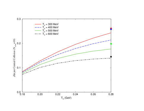
Figure 23: Predictions of kinetic model for $<J/\psi>$ with maximum temperature bounded by screening.

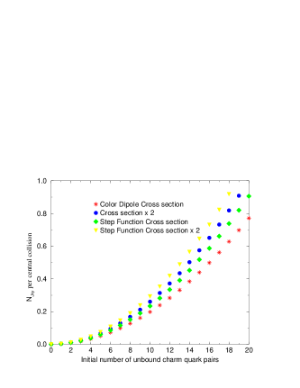
Figure 24: Variation of formation results with input cross section.

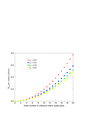
Figure 25: Variation of formation results with nonzero transverse expansion.

The new formation mechanism exhibits a significant sensitivity to the charm quark momentum distribution, as might be anticipated. In the calculation of the formation reactivity $\lambda_{F}$, momenta of any given pair will determine the reaction energy which in turn determines the effective value of the cross section. In addition, the charm quark energies enter into the formation rate through the usual formulas for non-collinear reactions. Thus we consider a large range of possibilities for these distributions. At one extreme, we model the distribution to simulate the initial production distribution from the pQCD calculations McGaughey et al. (1995). The transverse momentum $p_{T}$ distribution is taken to be Gaussian with a width of 1 $GeV^{2}$. The rapidity dependence is taken as flat, with the width of the plateau $\Delta$y = 4. We then allow for thermalization and energy loss processes in the deconfinement region by reducing the $\Delta$y, terminating at one unit. This corresponds approximately to the charm quark momentum distribution if complete thermalization were attained for all charm quarks in the central rapidity unit.

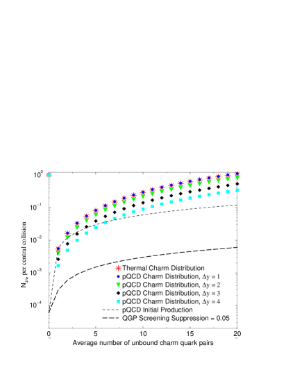
Figure 26: Predictions of kinetic model variation of $<J/\psi>$ due to charm momentum distributions.

The results of the calculations are shown in Figure 26. Shown are curves for final $N_{J/\psi}$ for central RHIC collisions as a function of $N_{c\bar{c}}$. All of the curves for various charm quark momentum distributions use zero initial $J/\psi$ and an initial temperature $T_{o}$ = 300 MeV to specify the gluon density and the lifetime of the deconfined region. Also shown for reference is the number of initial $J/\psi$ which would be produced without any nuclear or final state effects, which we approximate by $0.01N_{c\bar{c}}$ Gavai et al. (1995). The lowest curve just scales the initial production curve down by a factor 0.05, which is a typical suppression factor for RHIC conditions estimated from applications of suppression-only deconfinement models Vogt (1999). It is seen that over even this wide range of charm quark momentum distributions, the formation predictions are above the initial production estimate, thus indicating an enhancement in $J/\psi$. (This enhancement is even more extreme if the base is taken to be the suppressed initial number without any formation mechanism.)

We also show Figure 27 the equivalent energy dependence of these results, using RHIC conditions for the deconfinement properties but replacing $N_{c\bar{c}}$ by $\sqrt{s}$ from the pQCD expectations.

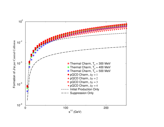
Figure 27: Predictions of kinetic model variation of $<J/\psi>$ as a function of $(\sqrt{s})_{NN}$ for RHIC conditions.

The centrality dependence will provide another prediction of this model. The most significant effect of varying centrality is to sweep through a range of $N_{c\bar{c}}$ from the centrality dependence of initial production as modeled by $T_{AA}(b)$, which we will change to the participant number dependence $T_{AA}(N_{p})$. However, a number of other components of the kinetic model will change with centrality, through the effect of nuclear geometry on the initial conditions and spatial properties of the deconfined region.

The initial temperature $T_{o}$ is expected to decrease with increasing impact parameter $b$, due to a decrease in the local energy density. We model the energy density in terms of the local density of participant nucleons in the transverse plane $n_{w}(b,s=0)$, which is shown in Figure 7. The dependence is then

$$T_{o}(b)=T_{o}(0)[n_{w}(b,s=0)/n_{w}(0,s=0)]^{1\over 4}$$ (22)

This dependence however is not very significant until the very peripheral region is reached.

One also needs the initial transverse size of the deconfined region. We model this area as the ratio of the participant number to the local density of participants, effectively using the fall-off of density to define the effective area within which the total number of participants would result if their density remained at its maximum value. Again this is not an absolute statement, since we normalize all of the centrality-dependent quantities to their values at b = 0.

$$A_{T}(b)=A_{T}(b=0)[N_{w}(b)n_{w}(0,s=0)/N_{w}(0)n_{w}(b,s=0)]$$ (23)

The results are most conveniently displayed in terms of the ratio $N_{J/\psi}/N_{c\bar{c}}$, which eliminates the trivial dependence on one power of $N_{c\bar{c}}$ expected in any physical mechanism for production of $J/\psi$. The centrality dependence of this ratio should be proportional to $N_{p}^{4/3-\alpha}$, where now $\alpha$ contains the net effect of the kinetic model centrality dependence.

The results for RHIC conditions are shown in Figure 28. The canonical $N_{c\bar{c}}$ = 10 value for central collisions is assumed, and required to vary with centrality as previously discussed. One sees the increase with large centrality due to the quadratic behavior of formation, which is a characteristic signature of this type of mechanism. It contrasts nicely with the initial production curve, which has the opposite behavior due to nuclear absorption of the initially-produced $J/\psi$. (The corresponding suppression-model curves would decrease even more rapidly with increasing centrality). The behavior for very peripheral collisions is probably an artifact of the procedure to determine the volume of the deconfinement region, and should not be taken at face value. One also sees the range of absolute values which result from variation of the charm quark momentum distribution. For sufficiently central collisions, all of these distributions predict final $J/\psi$ which exceed the initial production, i.e. enhancement.

Also shown for comparison are the statistical hadronization model calculations previously presented in Figure 17. The magnitudes are somewhat lower for the cases considered, but probably can be made compatible with some variation in parameters. The primary difference would appear to be the sharp increase for peripheral collisions due to the canonical corrections for small particle numbers.

Figure 29 shows the corresponding predictions for LHC. Here we have used $N_{c\bar{c}}$ = 200 for a central Pb-Pb collision at LHC. The range of charm quark momentum distributions has been increased to include up to $\Delta$y = 7 to account for the increased energy. It is clear that the absolute magnitudes of $N_{J/\psi}/N_{c\bar{c}}$ are larger than at RHIC. This is due to the increase in $N_{c\bar{c}}$ as contained in the quadratic dependence of the new formation mechanism.

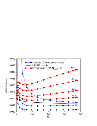
Figure 28: Predictions of kinetic model for $<J/\psi>$ over initial charm at RHIC energy.

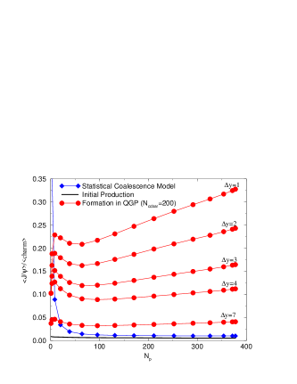
Figure 29: Predictions of kinetic model for $<J/\psi>$ over initial charm at LHC energy.

6 SUMMARY

Expectations based on general grounds for enhanced formation of heavy quarkonium in relativistic heavy ion collisions have been verified in two different models. In particular, one expects at RHIC and LHC to see an enhancement in the heavy quarkonium formation rate, even when compared to unsuppressed production via elementary nucleon-nucleon collisions in vacuum. The magnitude of this effect is expected to grow with the centrality of the heavy ion collision, just opposite to the predictions of various suppression scenarios. The physics bases for these models, however, are quite distinct. Their differences should manifest themselves in details of the magnitudes and centrality dependence. In this regard, it is essential to have a simultaneous measurement of open flavor production to serve as an unambiguous baseline.

References

- Altarelli (2002) Altarelli, G., Lectures on Perturbative QCD, these proceedings.
- Karsch (2002) Karsch, F., Lectures on Lattice QCD at Finite Temperature, these proceedings.
- Matsui and Satz (1986) Matsui, T., and Satz, H., Phys. Lett. B178, 416 (1986).
- M. C. Abreu (2000) M. C. Abreu et al., NA50 Collaboration, Phys. Lett. B477, 28–36 (2000).
- Vogt (1999) Vogt, R., Nucl Phys. A661, 250c (1999).
- McGaughey et al. (1995) McGaughey, P. L., Quack, E., Ruuskanen, P. V., Vogt, R., and Wang, X.-N., Int. J. Mod. Phys. A10, 2999–3042 (1995).
- Nason et al. (1988) Nason, P., Dawson, S., and Ellis, R. K., Nucl. Phys. B303, 607 (1988).
- Mangano et al. (1993) Mangano, M. L., Nason, P., and Ridolfi, G., Nucl.Phys. B405, 507–535 (1993).
- Frixone et al. (1994) Frixone, S., Mangano, M. L., Nason, P., and Ridolfi, G., Nucl.Phys. B431, 453–483 (1994).
- Vogt (2002) Vogt, R., “Systematics of heavy quark production at RHIC”, hep-ph/0203151 (2002).
- Zajc (2002) Zajc, W. A., Lectures on Phenix at RHIC, these proceedings.
- K. Adcox et. al. (2002) K. Adcox et al., PHENIX Collaboration, Phys. Rev. Lett. 88, 192303 (2002).
- Eskola et al. (1999) Eskola, K., Kolhinen, V., and Salgado, C., Eur. Phys. J. C9, 61–68 (1999).
- Białas et al. (1976) Białas, A., Bleszyński, M., and Czyz, W., Nucl. Phys. B111, 461 (1976).
- Margetis et al., NA49 Collaboration (1995) Margetis, S. et al., NA49 Collaboration, Nucl. Phys. A590, 355c (1995).
- Thews (2002) Thews, R. L., Nucl. Phys. A702, 341–345 (2002).
- Wang and Gyulassy (2001) Wang, X.-N., and Gyulassy, M., Phys. Rev. Lett. 86, 3496–3499 (2001).
- Gavai et al. (1995) Gavai, R., Kharzeev, D., Satz, H., Schuler, G., Sridhar, K., and Vogt, R., Int. J. Mod. Phys. A10, 3043–3070 (1995).
- M.M.Agarwal et al. (WA98 Collaboration) Agarwal, M. M. et al., WA98 Collaboration, Eur. Phys. J. C18, 651–663 (2001).
- K. Adcox etal Phenix Collaboration (2001) Adcox, K. et al., PHENIX Collaboratiion, Phys. Rev. Lett. 87, 052301 (2001).
- B. B. Back (2002) Back, B. B. et al., PHOBOS Collaboration, Phys. Rev. Lett. 88, 022302 (2002).
- I. G. Bearden (2001) Bearden, I. G. et al., BRAHMS Collaboration, nucl-ex/0112001.
- Kharzeev et al. (1997) Kharzeev, D., Lourenco, C., Nardi, M., and Satz, H., Z. Phys. C74, 307–318 (1997).
- Braun-Munzinger et al. (2001) Braun-Munzinger, P., Magestro, D., Redlich, K., and Stachel, J., Phys. Lett. B518, 41–46 (2001).
- Sorge et al. (1997) Sorge, H., Shuryak, E., and Zahed, I., Phys. Rev. Lett. 79, 2775–2778 (1997).
- Braun-Munzinger and Stachel (2000) Braun-Munzinger, P., and Stachel, J., Phys. Lett. B490, 196–202 (2000).
- Braun-Munzinger and Stachel (2001) Braun-Munzinger, P., and Stachel, J., Nucl. Phys. A690, 119–126 (2001).
- Gorenstein et al. (2001) Gorenstein, M., Kostyuk, A., Stocker, H., and Greiner, W., Phys. Lett. B509, 277–282 (2001).
- Redlich et al. (2002) Redlich, K., Koch, V., and Tounsi, A., Nucl. Phys. A702, 326–335 (2002).
- Cleymans et al. (1991) Cleymans, J., Redlich, and Suhonen, E., Z. Phys. C51, 137–141 (1991).
- Gorenstein et al. (2001) Gorenstein, M., Kostyuk, A., Stocker, H., and Greiner, W., hep-ph/0110269.
- M. C. Abreu (2002) Abreu, M. C. et al., NA38/50 Collaboration, Nucl. Phys. A698, 539–542 (2002).
- Grandchamp and Rapp (2001) Grandchamp, L., and Rapp, R., Phys. Lett. B523, 60–66 (2001).
- Thews et al. (2001) Thews, R. L., Schroedter, M., and Rafelski, J., Phys. Rev. C63, 054905 (2001).
- Thews and Rafelski (2002) Thews, R. L., and Rafelski, J., Nucl. Phys. A698, 575–578 (2002).
- Kharzeev and Satz (1994) Kharzeev, D., and Satz, H., Phys. Lett. B334, 155–162 (1994).
- Sucipto and Thews (2002) Sucipto, E., and Thews, R. L., work in progress.
- Rafelski et al. (1996) Rafelski, J., Letessier, J., and Tounsi, A., Heavy Ion Phys. 4, 181–192 (1996).
- Peskin (1979) Peskin, M. E., Nucl Phys. B156, 365 (1979).
- Bhanot and Peskin (1979) Bhanot, G., and Peskin, M. E., Nucl Phys. B156, 391 (1979).