1 Introduction

An important unresolved question in strong interaction physics concerns the parameterization of power-suppressed long-distance effects to hard processes that do not admit an operator product expansion (OPE). For a large class of processes of this type the principal difficulty arises from the presence of collinear modes, i.e. highly energetic, but nearly massless particles.

In a series of papers [1, 2, 3, 4, 5] Bauer et al. have developed an effective field theory framework that allows one for the first time to formulate the problem of soft-collinear factorization in terms of fields and operators, rather than the factorization properties of Feynman diagrams. Assuming that the field content of the effective theory correctly includes all long-distance modes, the effective field theory formulation simplifies or renders more transparent the factorization proofs that form the conceptual basis of high-energy QCD phenomenology [6, 7]. The effective theory has been formulated only to leading order in an expansion in the hard scale up to now, as have been the diagrammatic factorization methods.

In this paper we extend the formulation of soft-collinear effective theory to second order in a power series in the inverse of the hard scale. We give the effective Lagrangian and the expansion of “currents” that produce collinear particles in heavy quark decay. This is the first step towards a theory of power corrections to hard processes that do not admit an OPE. Previous approaches to this problem include the renormalon approach (reviewed in [8]), where power corrections have been identified through the asymptotics of the perturbative series at leading power. This approach is severely limited since only those power corrections can be included that are related through renormalization to operators appearing already at leading power. The effective theory approach is free from this limitation.

The outline of this paper is as follows: in Section 2 we set up the notation, power counting rules, fields and gauge transformations of the effective theory. In Sections 3 and 4 we derive the effective Lagrangian of soft-collinear effective theory (SCET) and the effective heavy-to-light currents, respectively, to second order in the expansion parameter of the effective theory. We then discuss in Section 5 power-suppressed effects that break the symmetries between heavy-to-light meson transition form factors at large recoil, extending previous work of two of us [9] on perturbative symmetry-breaking corrections. We conclude in Section 6.

2 Power counting and fields

We begin with detailing the power counting rules and fields from which the effective theory will be constructed. This discussion is a repetition of previous work [2], using our preferred notation, except for two aspects. Bauer et al. use a hybrid momentum-position space representation in their formulation of the effective theory, where collinear fields are labelled by the large part of the collinear momentum of the particles they create and destroy. The corresponding derivatives are replaced by “label operators”. We find it more convenient, especially for the extension to power corrections, to stay within the conventional position space representation, where the effective field theory can be formulated in more familiar field theory terminology. The second modification concerns the definition of gauge transformations and Wilson lines, and is necessary to extend the theory beyond leading order. The position space representation also requires that one expands ultrasoft fields in their position arguments. This will be explained in Section 3.

2.1 Kinematical definitions

The effective theory is designed to expand a physical process in powers of a small ratio of scales, $\lambda$. In perturbative computations the relevant scales are determined by specifying the external momenta of certain Green functions. In a real hadronic process these external momentum configurations are enforced by hadronic wavefunctions or the selection of specific final states by the observer. The situation we are interested in here consists of a cluster of nearly collinear particles moving with large momentum of order $m$ into a direction $n_{-}$, such that the total invariant mass is of order $(m\lambda)^{2}$. This acquires a Lorentz-invariant meaning if there is a source for collinear particles. We may think for instance of a heavy quark of mass $m$ at rest, which decays semileptonically into a set of partons with large energy and small invariant mass, as is relevant to exclusive decays, see Figure 1. More complicated situations often arise in jet physics, where the final state can consist of several clusters moving into different well-separated directions. However, in this paper we restrict ourselves to the case of a single direction $n_{-}$.

Figure 1: Kinematics of heavy quark decay into a single cluster of collinear and ultrasoft particles.

We decompose the momentum $p$ of a collinear particle as

$$p^{\mu}=(n_{+}p)\,\frac{n_{-}^{\mu}}{2}+p_{\perp}^{\mu}+(n_{-}p)\frac{n_{+}^{\mu}}{2},$$ (1)

where $n_{\pm}^{\mu}$ are two light-like vectors, $n_{+}^{2}=n_{-}^{2}=0$ with $n_{+}n_{-}=2$. The individual momentum components are assumed to have the following scaling behaviour,

$$n_{+}p\sim m,\quad p_{\perp}\sim m\lambda,\quad n_{-}p\sim m\lambda^{2},$$ (2)

such that $p^{2}\sim m^{2}\lambda^{2}$ as required. In the following we shall put $m=1$ in scaling relations such as (2), understanding that the dimension of any quantity is restored by inserting the appropriate power of $m$.

The invariant mass of the final state is not altered if we add to it a particle with momentum $k$ whose components are all of order $\lambda^{2}$. The effective theory therefore also contains such ultrasoft particles. The effective theory does not contain soft particles, whose momentum components are all of order $\lambda$, as external states, since adding such a particle (with momentum $k$) to a cluster of collinear particles with momentum $p$ implies an invariant mass $(p+k)^{2}\sim\lambda$ in contradiction with our kinematical assumption.

2.2 Fields

We construct an effective field theory by introducing separate collinear and ultrasoft fields that destroy and create collinear and ultrasoft (anti-)particles, respectively. It follows that an ultrasoft field $\phi_{\rm us}(x)$ varies significantly only over distances of order $x\sim 1/\lambda^{2}$, so derivatives acting on these fields scale as

$$\partial_{\mu}\phi_{\rm us}\sim\lambda^{2}\phi_{\rm us}.$$ (3)

Collinear fields have significant variations over $n_{-}x\sim 1$, and $x_{\perp}\sim 1/\lambda$. Derivatives acting on collinear fields $\phi_{c}$ therefore scale as

$$n_{+}\partial\phi_{c}\sim\phi_{c},\quad\partial_{\perp}\phi_{c}\sim\lambda\phi_{c},\quad n_{-}\partial\phi_{c}\sim\lambda^{2}\phi_{c}.$$ (4)

The effective theory is constructed to reproduce the Green functions of QCD under the kinematical assumption above as an expansion in $\lambda$. With a large scale $m$ present, quantum fluctuations with virtuality $m^{2}$ also contribute. These hard modes can be integrated out perturbatively. In practice, this amounts to Taylor-expanding the loop integrals in $\lambda$, assuming that all loop momenta scale as $m$. The effective theory accounts for those loop momentum regions where this expansion breaks down, i.e. for those configurations where some propagators become on-shell as $\lambda\to 0$. For the given kinematics this leads to the collinear, soft and ultrasoft modes defined above. Since soft modes do not appear as external states, they can be integrated out. This will be understood in the following, but since (with the exception of Section 3.4) this paper is concerned with power corrections in $\lambda$ at tree level, the details of integrating out soft modes will not be important.

In the case of QCD we introduce collinear and ultrasoft quark and gluon fields and assign a scaling rule to them. A collinear quark field has two large and two small components. The decomposition of the spinor is as follows:

$$\psi_{c}(x)=\xi(x)+\eta(x),\qquad\xi(x)\equiv\frac{\not\!n_{-}\!\!\not\!n_{+}}{4}\,\psi_{c}(x),\quad\eta(x)\equiv\frac{\not\!n_{+}\!\!\not\!n_{-}}{4}\,\psi_{c}(x),$$ (5)

where $(n\hskip-4.49997pt/_{\mp}n\hskip-4.49997pt/_{\pm})/4$ are projection operators, and $n\hskip-4.49997pt/_{-}\xi=n\hskip-4.49997pt/_{+}\eta=0$. The scaling of these components is obtained from the projection of the QCD quark propagator. For $\xi$ fields

$$\langle 0|T\xi(x)\bar{\xi}(y)|0\rangle=\frac{\not\!n_{-}\!\!\not\!n_{+}}{4}\,\langle 0|T\psi_{c}(x)\bar{\psi}_{c}(y)|0\rangle\frac{\not\!n_{+}\!\!\not\!n_{-}}{4}=\int\frac{d^{4}p}{(2\pi)^{4}}\,\frac{n\hskip-4.49997pt/_{-}}{2}\frac{in_{+}p}{p^{2}+i\epsilon}\,e^{-ip(x-y)}.$$ (6)

For collinear momentum $p$ the right-hand side is of order $\lambda^{2}$. From this and the analogous equation for $\eta$ with $n_{-}$ and $n_{+}$ interchanged, we conclude

$$\xi\sim\lambda,\qquad\eta\sim\lambda^{2}.$$ (7)

The small $\eta$ field will later be integrated out. The corresponding argument for an ultrasoft quark field, which we denote by $q$, dictates

$$q\sim\lambda^{3}$$ (8)

for all components of the spinor. Here $k^{2}\sim\lambda^{4}$ and $d^{4}k\sim\lambda^{8}$ for ultrasoft momentum has been used.

The scaling of the collinear gluon field is determined by projecting the gluon propagator (in a covariant gauge with gauge fixing parameter $\alpha$)

$$\langle 0|TA_{c}^{\mu}(x)A_{c}^{\nu}(y)|0\rangle=\int\frac{d^{4}p}{(2\pi)^{4}}\,\frac{i}{p^{2}+i\epsilon}\left[-g^{\mu\nu}+(1-\alpha)\,\frac{p^{\mu}p^{\nu}}{p^{2}}\right]e^{-ip(x-y)}$$ (9)

on its various components. This requires the gluon fields to scale identically to a collinear momentum,

$$n_{+}A_{c}\sim 1,\quad A_{\perp c}\sim\lambda,\quad n_{-}A_{c}\sim\lambda^{2}.$$ (10)

For an ultrasoft gluon field,

$$A_{\rm us}^{\mu}\sim\lambda^{2}$$ (11)

for all components. Comparing the scaling properties of derivatives with those of gluon fields we see that collinear and ultrasoft covariant derivatives have homogeneous scaling rules: the terms in a covariant collinear derivative $iD_{c}^{\mu}\phi_{c}=(i\partial^{\mu}+gA_{c}^{\mu})\phi_{c}$ acting on a collinear field all scale in the same manner. A corresponding statement holds for $iD_{\rm us}^{\mu}\phi_{\rm us}=(i\partial^{\mu}+gA_{\rm us}^{\mu})\phi_{\rm us}$ acting on ultrasoft fields.

In cases where collinear particles are produced in the decay of a heavy quark, we also need an effective heavy quark field. When collinear modes interact with a nearly on-shell heavy quark, the heavy quark will subsequently be off-shell by an amount of order 1. These off-shell modes are removed from the effective theory, and heavy quarks interact only with ultrasoft gluons. It is therefore appropriate to remove the large component $mv$ of a heavy quark momentum $p=mv+k$ just as in heavy quark effective theory by introducing the field

$$h_{v}(x)=\frac{1+v\hskip-4.49997pt/}{2}\,e^{im\,v\cdot x}\,Q(x)$$ (12)

which varies significantly only over distances $x\sim 1/\lambda^{2}$, since $k$ is ultrasoft. The momentum space propagator of $h_{v}$ is $1/(vk)$, so $h_{v}\sim\lambda^{3}$ just as the massless ultrasoft quark field.

We finally need to assign a scaling to the integration element $d^{4}x$ in each term of the effective action, which must reproduce the power counting for Feynman graphs in momentum space. Expressing each field through its Fourier transform, $\phi_{i}(x)=\int d^{4}p_{i}\,e^{-ixp_{i}}\tilde{\phi}_{i}(p_{i})$, we see that the integral over $x$ in the action eliminates one momentum integral

$$\int d^{4}x\,\left(\prod_{i=1}^{n}d^{4}p_{i}\right)\exp(-ix\sum_{i=1}^{n}p_{i})=\int\left(\prod_{i=1}^{n-1}d^{4}p_{i}\right)d^{4}p_{n}\,(2\pi)^{4}\delta^{(4)}(p_{n}+\sum_{i=1}^{n-1}p_{i})$$ (13)

in a term with $n$ fields. The scaling of $d^{4}x$ is thus $1/\lambda^{4}$ if the eliminated integral $\int d^{4}p_{n}$ is over a collinear momentum, and $1/\lambda^{8}$ if it is ultrasoft. For products involving both collinear and ultrasoft fields, one must choose the eliminated momentum to be collinear and thus count $d^{4}x$ as $1/\lambda^{4}$. This is because eliminating the ultrasoft integration in an integral such as $\int d^{4}p_{1c}\,d^{4}p_{2c}\,d^{4}p_{3us}$ would no longer ensure that the momentum $p_{3}=-(p_{1c}+p_{2c})$ is ultrasoft.

2.3 Gauge transformations

The effective theory must have a remnant gauge symmetry from gauge functions $U(x)$ that can themselves be classified as collinear or ultrasoft.

It is clear that ultrasoft fields cannot transform under collinear gauge transformations, since this would turn the ultrasoft field into a collinear field. Under ultrasoft gauge transformations ultrasoft fields transform in the usual way. The collinear quark field $\xi$ is also multiplied by $U$ under both collinear and ultrasoft gauge rotations. Since ultrasoft gluon fields can be added to collinear gluon fields without changing the character of the collinear field, ultrasoft gluons can be viewed as slowly varying background fields for the collinear ones. Then $A_{c}$ transforms covariantly under ultrasoft gauge transformations, while it transforms inhomogeneously under collinear gauge transformations, but with the derivative replaced by the covariant derivative with respect to the background field. These properties are summarized by:

$$\begin{array}[]{lll}\mbox{collinear: }&\displaystyle A_{c}\to U_{c}\,A_{c}\,U^{\dagger}_{c}+\frac{i}{g}\,U_{c}\left[D_{\rm us},U^{\dagger}_{c}\right],&\xi\to U_{c}\,\xi,\\[5.69046pt] &A_{\rm us}\to A_{\rm us},&q\to q,\\[8.5359pt] \mbox{ultrasoft: }&A_{c}\to U_{\rm us}\,A_{c}\,U^{\dagger}_{\rm us},&\xi\to U_{\rm us}\,\xi,\\[2.84544pt] &\displaystyle A_{\rm us}\to U_{\rm us}\,A_{\rm us}\,U^{\dagger}_{\rm us}+\frac{i}{g}\,U_{\rm us}\left[\partial,U^{\dagger}_{\rm us}\right],&q\to U_{\rm us}\,q,\end{array}$$ (18)

where $D^{\mu}_{\rm us}=\partial^{\mu}-igA^{\mu}_{\rm us}$ is an ultrasoft covariant derivative. The heavy quark field $h_{v}$ has transformation properties identical to $q$. Note that the sum $A_{c}+A_{\rm us}$ transforms in the standard way under both types of gauge transformations.

Under collinear transformations the components $n_{+}A_{c}$ and $A_{c\perp}$ acquire a component of order $\lambda^{2}$ due to the ultrasoft gluon field in the transformation rule. Ultrasoft gauge transformations are homogeneous in $\lambda$, i.e. all terms in the transformation law have the same scaling in $\lambda$, but operators such as $iD_{\perp c}\xi$ transform inhomogeneously in $\lambda$ under ultrasoft transformations as well. A consequence of this is that operators that have a definite scaling with $\lambda$ are in general not covariant with respect to gauge transformations as defined above, but should be combined with higher-order terms in the $\lambda$ expansion into a gauge-covariant object. In the following, we will always keep gauge invariance manifest as far as possible, before we switch to the strict $\lambda$ expansion of the effective operators.

2.4 Wilson lines

The effective theory makes extensive use of various Wilson lines. We collect the relevant definitions and properties here. The basic Wilson line is defined as

$$W(x)=P\exp\left(ig\int_{-\infty}^{0}\!ds\,n_{+}A(x+sn_{+})\right),$$ (19)

where $P$ denotes path-ordering defined as $P[A(x)A(x+sn_{+})]=A(x)A(x+sn_{+})$, if $s<0$. Here $A=A_{c}+A_{\rm us}$ denotes the sum of the collinear and ultrasoft gluon fields. The Wilson line is a unitary operator, $WW^{\dagger}=W^{\dagger}W=1$, and has the following useful properties

$$in_{+}D\,W=W\,in_{+}\partial,\qquad(in_{+}D+i\epsilon)^{-1}=W\,(in_{+}\partial+i\epsilon)^{-1}\,W^{\dagger}.$$ (20)

Under general gauge transformations $U(x)$, $W(x)$ transforms as

$$W(x)\to U(x)W(x)U^{\dagger}(x-\infty\,n_{+}).$$ (21)

The particular form of the transformation matrix at $n_{-}x\to\infty$ turns out to be irrelevant, since Wilson lines always appear in combinations where the transformation at infinite distance drops out. An example is the finite-distance Wilson line $W(x)W^{\dagger}(x+sn_{+})$, which corresponds to a line integral between $x+sn_{+}$ and $x$, and which transforms as

$$W(x)W^{\dagger}(x+sn_{+})\to U(x)W(x)W^{\dagger}(x+sn_{+})U^{\dagger}(x+sn_{+}).$$ (22)

It is therefore consistent to choose $U(x-\infty\,n_{+})=1$ and this choice will be adopted in the following. Under collinear and ultrasoft gauge transformations we then have

$$W\to U_{c}\,W,\qquad W\to U_{\rm us}\,W.$$ (23)

We also introduce the ultrasoft Wilson line $Z$ that is defined as in (19) but with the full gauge field replaced by the ultrasoft one, $A_{\rm us}$. This Wilson line is invariant under collinear gauge transformations and transforms as

$$Z\to U_{\rm us}\,Z$$ (24)

under ultrasoft ones. A particularly important quantity is the product of Wilson lines, $W\!Z^{\dagger}$. It fulfills the equalities

$$in_{+}D\,W\!Z^{\dagger}=W\!Z^{\dagger}\,in_{+}D_{\rm us},\qquad(in_{+}D+i\epsilon)^{-1}W\!Z^{\dagger}=W\!Z^{\dagger}\,(in_{+}D_{\rm us}+i\epsilon)^{-1}$$ (25)

and transforms as

$$W\!Z^{\dagger}\to U_{c}\,W\!Z^{\dagger},\qquad W\!Z^{\dagger}\to U_{\rm us}\,W\!Z^{\dagger}\,U^{\dagger}_{\rm us}$$ (26)

under collinear and ultrasoft gauge transformations. Furthermore we specify the two limiting cases

$$W\!Z^{\dagger}\to 1\qquad\mbox{for $A_{c}\to 0$},$$

$$W\!Z^{\dagger}\to W_{c}\equiv P\exp\left(ig\int_{-\infty}^{0}\!ds\,n_{+}A_{c}(x+sn_{+})\right)\qquad\mbox{for $A_{\rm us}\to 0$}.$$ (27)

Note that the purely collinear Wilson line $W_{c}$ defined above does not have a simple behaviour under gauge transformations as soon as ultrasoft gauge fields are taken into account.

The integration measure $ds$ in the definition of the Wilson line counts as $1/\lambda^{2}$ if the integrand contains ultrasoft fields only, but it counts as $1$, if the integrand contains a collinear field. This can be seen in the momentum space representation, where $\int ds$ corresponds to $1/(n_{+}p)$. It follows that all three Wilson lines, $W$, $Z$, $W_{c}$ count as order $1$. In contrast to $Z$ and $W_{c}$, however, $W$ is not homogeneous in $\lambda$ due to the occurrence of both, collinear and ultrasoft gauge fields. Due to the case-dependent counting rule for $ds$, $W$ does not even have a useful expansion in $\lambda$, where ultrasoft fields should appear as corrections. What we actually need below is the $\lambda$ expansion of the product $W\!Z^{\dagger}$, which is well-behaved. To construct the expansion we rewrite (25) as

$$in_{+}D_{c}\,W\!Z^{\dagger}=\Big{[}W\!Z^{\dagger},gn_{+}A_{\rm us}\Big{]},$$ (28)

where the derivative acts only on $W\!Z^{\dagger}$, and solve this equation iteratively with the “boundary condition” $W\!Z^{\dagger}\to 1$ when $A_{c}\to 0$. We obtain

$$W\!Z^{\dagger}(x)=W_{c}(x)+W_{c}\,(in_{+}\partial+i\epsilon)^{-1}\,W_{c}^{\dagger}\Big{[}W_{c},gn_{+}A_{\rm us}\Big{]}+{\cal O}(\lambda^{4})$$

$$=W_{c}(x)\left(1-i\int_{-\infty}^{0}ds\,W_{c}^{\dagger}(x+sn_{+})\Big{[}W_{c},gn_{+}A_{\rm us}\Big{]}(x+sn_{+})\right)+{\cal O}(\lambda^{4}),$$ (29)

where we used that the inverse of $in_{+}\partial$, here defined with a $+i\epsilon$-prescription, acts as

$$\frac{1}{in_{+}\partial+i\epsilon}\,\phi(x)=-i\int_{-\infty}^{0}\!ds\,\phi(x+sn_{+}).$$ (30)

Note that the commutator term in (29), $[W_{c},gn_{+}A_{\rm us}]=[W_{c}-1,gn_{+}A_{\rm us}]$, has at least one collinear field when the exponential is expanded, and therefore counts as a collinear field. The integration element $ds$ then counts as $O(1)$, which is crucial to ensure that the second term in (29) is $\lambda^{2}$ suppressed. In a similar manner one sees that $(1-W\!Z^{\dagger})$ is also a collinear field. On the other hand, the Wilson lines $W_{c}$ and $W\!Z^{\dagger}$ without the unity subtracted do not qualify as collinear fields and expressions such as

$$\int_{-\infty}^{0}ds\,[W\!Z^{\dagger}f_{\rm us}](x+sn_{+})$$ (31)

where $f_{\rm us}(x)$ denotes a product of only ultrasoft fields, do not have a well-defined $\lambda$ scaling behaviour and must be avoided.

3 Effective Lagrangian

In this section we construct the effective Lagrangian for collinear and ultrasoft quarks and gluons including all interactions suppressed by one or two powers of $\lambda$. We shall first derive the Lagrangian in a form that is manifestly gauge-invariant, but where the operators do not have a homogeneous $\lambda$ scaling. Each operator generates a series in $\lambda$ and is counted by its largest term in the $\lambda$ expansion. In a second step each operator is expanded in a series of terms each of which has a definite $\lambda$ scaling. We then show that the effective Lagrangian obtained by tree level matching is not renormalized to any order in the coupling $\alpha_{s}$, provided a Poincaré-invariant regularization procedure such as dimensional regularization can be chosen. This remarkable non-renormalization property extends to all orders in $\lambda$.

3.1 Collinear Lagrangian

We begin with deriving the Lagrangian for collinear quarks interacting with collinear and ultrasoft gluons, neglecting the ultrasoft quark field for now. This will be corrected for in the next subsection. The QCD Lagrangian for massless quarks is

$${\cal L}_{c}=\bar{\psi}_{c}\left(i\!\not\!\!D+i\epsilon\right)\psi_{c},$$ (32)

where $\psi_{c}$ is a four-component spinor, assumed to describe a nearly on-shell particle with large momentum in the $n_{-}$ direction. The covariant derivative is defined as $D=\partial-igA$, where $A$ is the sum of the collinear and ultrasoft gluon fields. Inserting the decomposition (5) into the QCD Lagrangian, we obtain

$${\cal L}_{c}=\bar{\xi}\,\frac{\not\!n_{+}}{2}\,in_{-}D\,\xi+\bar{\eta}\,\frac{\not\!n_{-}}{2}\,in_{+}D\,\eta+\bar{\xi}\left(i\!\not\!\!D_{\perp}+i\epsilon\right)\eta+\bar{\eta}\left(i\!\not\!\!D_{\perp}+i\epsilon\right)\xi.$$ (33)

Here we indicated explicitly that the $i\epsilon$ prescription of the original Lagrangian is attached to the transverse derivatives. Having this in mind, we will suppress it in the following.

We proceed by integrating out the small field $\eta$ from the path integral. Since the Lagrangian is quadratic this amounts to solving the classical equation of motion, which gives

$$\eta(x)=-\frac{\not\!n_{+}}{2}\left(in_{+}D+i\epsilon\right)^{-1}i\!\not\!\!D_{\perp}\,\xi(x)=i\,\frac{\not\!n_{+}}{2}\,W(x)\int_{-\infty}^{0}ds\,\left[W^{\dagger}\,i\!\not\!\!D_{\perp}\,\xi\right](x+sn_{+}),$$ (34)

where we have used (20) and (30) to obtain the second equality. This is consistent with $\eta\sim\lambda^{2}$ as stated in (7). In writing the solution for $\eta$ we have defined the inverse of $in_{+}D$ with a $+i\epsilon$ prescription. This prescription is not given by the QCD Lagrangian, and we could have chosen the opposite sign or a principal value prescription. The ambiguity in this prescription cancels out in physical quantities, but the prescription is needed to define individual terms that appear in the calculation. This is similar to the need to define a treatment of spurious singularities of gluon propagators in light-cone gauge. The functional determinant of the operator $in_{+}D$, which appears upon integrating out $\eta$, amounts to an irrelevant gauge-field independent constant and can be dropped. To see this, note that the determinant is gauge-invariant so that we can evaluate it in light-cone gauge $n_{+}A=0$, where $in_{+}D=in_{+}\partial$. The result for the collinear quark Lagrangian is then simply given by inserting (34) into (33), and reads

$${\cal L}_{c} = \bar{\xi}\,in_{-}D\,\frac{n\hskip-4.49997pt/_{+}}{2}\,\xi+\bar{\xi}\,iD\hskip-5.89996pt/_{\perp}\frac{1}{in_{+}D+i\epsilon}\,iD\hskip-5.89996pt/_{\perp}\frac{n\hskip-4.49997pt/_{+}}{2}\,\xi$$ (35)

$$= \bar{\xi}(x)\,in_{-}D\,\frac{n\hskip-4.49997pt/_{+}}{2}\,\xi(x)+i\int_{-\infty}^{0}\!ds\,\bigg{[}\bar{\xi}\,i\overleftarrow{D\hskip-5.89996pt/}_{\perp}W\bigg{]}(x)\,\bigg{[}W^{\dagger}\,iD\hskip-5.89996pt/_{\perp}\frac{n\hskip-4.49997pt/_{+}}{2}\,\xi\bigg{]}(x+sn_{+}),$$

where $\overleftarrow{D}=\overleftarrow{\partial}+igA$ is the covariant derivative acting to the left. Note that the effective Lagrangian is formally not hermitian because of the $+i\epsilon$ prescription on $(in_{+}D)^{-1}$, which also implies that products of fields $\phi(x_{1})\cdots\phi(x_{n})$ are “ordered” along the $n_{+}$ direction, $n_{-}x_{1}\geq\ldots\geq n_{-}x_{n}$. The hermitian conjugate of the Lagrangian corresponds to the $-i\epsilon$ prescription. The non-hermiticity is of no consequence, since it is related to modes with $n_{+}p=0$, while collinear modes have $n_{+}p\sim 1$. Concretely, the non-local quark-gluon vertices that follow from expanding the Wilson line in the gauge field individually contain factors $1/(n_{+}p+i\epsilon)$, but these unphysical poles cancel in the sum of all diagrams.

The Lagrangian (35) is equivalent to the Lagrangian derived in [2] in the hybrid momentum-position space representation, when $W$ is replaced by the collinear Wilson line $W_{c}$ and when the ultrasoft gluon field is neglected in $iD\hskip-5.89996pt/_{\perp}$. Using the power counting rules developed in Section 2 it is easy to see that this corresponds to the leading term in the expansion in $\lambda$. The result (35) is the exact collinear Lagrangian to all orders in $\lambda$. It is manifestly collinear and ultrasoft gauge-invariant, which follows from the transformation properties (23) of $W$, or directly from the first line of (35). The expansion of (35) in $\lambda$ will be discussed below, after ultrasoft quarks have been included.

The derivation of the Lagrangian did in fact not require the assumption that $\psi_{c}$ or $\xi$ are collinear fields. It can also be viewed as integrating out two of the components of the quark spinor field in full QCD, with $n_{-}$ and $n_{+}$ chosen arbitrarily. This makes it clear that the Lagrangian (35) is equivalent to the quark Lagrangian of full QCD, including all hard and soft modes (and ultrasoft quarks), provided we consider $\xi$ as a field that destroys and creates all these modes, not only collinear ones. This peculiar result follows because the notion of a collinear particle has no Lorentz-invariant meaning in the absence of sources that create such particles. The collinear Lagrangian must therefore exactly reproduce the Green functions of full QCD (projected appropriately as in (6)), when they are evaluated in a frame where all particles have large momentum in the $n_{-}$ direction. This interpretation is also confirmed by the observation that the equation of motion that follows from (35) and the expression for $\eta$ is identical to what one obtains in a treatment of full QCD in the infinite momentum frame [11] or in light-cone quantization [12, 13]. In the following we shall not pursue this interpretation further since the Lagrangian will eventually be coupled to sources of collinear particles and we are interested in performing an expansion in $\lambda$, which implies that fields must be classified as collinear and ultrasoft.

3.2 Including ultrasoft quarks

We now incorporate the ultrasoft light quark field, $q$, into the effective Lagrangian. The QCD Lagrangian gives rise to the following tree-level interactions among collinear and ultrasoft fields:

$${\cal L} = \bar{\xi}\,\frac{n\hskip-4.49997pt/_{+}}{2}\,in_{-}D\,\xi+\bar{\eta}\,\frac{n\hskip-4.49997pt/_{-}}{2}\,in_{+}D\,\eta+\bar{\xi}\,iD\hskip-5.89996pt/_{\perp}\,\eta+\bar{\eta}\,iD\hskip-5.89996pt/_{\perp}\,\xi$$ (36)

$$+\,\bar{\xi}\,gA\hskip-5.89996pt/_{c}\,q+\bar{\eta}\,gA\hskip-5.89996pt/_{c}\,q+\bar{q}\,gA\hskip-5.89996pt/_{c}\,\xi+\bar{q}\,gA\hskip-5.89996pt/_{c}\,\eta+\bar{q}\,iD\hskip-5.89996pt/_{\rm us}\,q,$$

where $iD_{\rm us}=i\partial+gA_{\rm us}$. Note that terms such as $\bar{\xi}\,iD\hskip-5.89996pt/_{\rm us}\,q$ vanish by momentum conservation enforced by the $d^{4}x$ integral in the action. Collinear gauge invariance is not manifest in (36). We now integrate out the $\eta$ field as before and order the terms in an expansion in $\lambda$. In this process we use the field equation for $\xi$, which is equivalent to a field redefinition such that the final Lagrangian will be manifestly gauge-invariant under the transformations (18).

Since the Lagrangian (36) is still quadratic in the $\eta$ field, it can be integrated out straightforwardly. The $\eta$ field is now given by

$$\eta = -\frac{1}{in_{+}D+i\epsilon}\,\frac{n\hskip-4.49997pt/_{+}}{2}\left(iD\hskip-5.89996pt/_{\perp}\xi+gA\hskip-5.89996pt/_{c}\,q\right).$$ (37)

In the following $(in_{+}D)^{-1}$ will always be understood with a $+i\epsilon$ prescription. Inserting (37) into (36) results in

$${\cal L} = {\cal L}_{c}+{\cal L}_{\rm us}+\bar{\xi}\,gA\hskip-5.89996pt/_{c}\,q+\bar{q}\,gA\hskip-5.89996pt/_{c}\,\xi-\bar{q}\,gA\hskip-5.89996pt/_{c}\,\frac{1}{in_{+}D}\frac{n\hskip-4.49997pt/_{+}}{2}\,gA\hskip-5.89996pt/_{c}\,q$$ (38)

$$-\,\bar{\xi}\,iD\hskip-5.89996pt/_{\perp}\,\frac{1}{in_{+}D}\frac{n\hskip-4.49997pt/_{+}}{2}\,gA\hskip-5.89996pt/_{c}\,q-\bar{q}\,gA\hskip-5.89996pt/_{c}\,\frac{1}{in_{+}D}\frac{n\hskip-4.49997pt/_{+}}{2}\,iD\hskip-5.89996pt/_{\perp}\xi,$$

with ${\cal L}_{c}$ given by (35), and ${\cal L}_{\rm us}=\bar{q}\,iD\hskip-5.89996pt/_{\rm us}\,q$ the purely ultrasoft Lagrangian. Note that both ${\cal L}_{c}$ and ${\cal L}_{\rm us}$ are order one terms in the action, since the integration measure $d^{4}x$ counts as $\lambda^{-4}$ in $\int d^{4}x\,{\cal L}_{c}$ but counts as $\lambda^{-8}$ in $\int d^{4}x\,{\cal L}_{\rm us}$, where the integrand involves only ultrasoft fields. The mixed terms in the Lagrangian are subleading contributions in $\lambda$ to the action, beginning at order $\lambda$.

The new terms at order $\lambda$ involving the ultrasoft quark field are

$${\cal L}^{(1)} = \bar{\xi}\left(gA\hskip-5.89996pt/_{\perp c}-iD\hskip-5.89996pt/_{\perp}\,\frac{1}{in_{+}D}\,gn_{+}A_{c}\right)q+\bar{q}\left(gA\hskip-5.89996pt/_{\perp c}-gn_{+}A_{c}\,\frac{1}{in_{+}D}\,iD\hskip-5.89996pt/_{\perp}\right)\xi.$$ (39)

This can be simplified with the identity

$$\frac{1}{in_{+}D}\,gn_{+}A_{c}\,\phi_{\rm us} = (1-W\!Z^{\dagger})\,\phi_{\rm us}-\frac{1}{in_{+}D}\,(1-W\!Z^{\dagger})\,in_{+}D_{\rm us}\,\phi_{\rm us},$$ (40)

which follows from (25) and is easily verified by acting with $in_{+}D$ from the left. The key point to note about this identity is that the first term on the right-hand side is of order $1$, but the second is of order $\lambda^{2}$ due to the ultrasoft derivative. For this to be correct it is essential that $(1-W\!Z^{\dagger})$ is a collinear field, which ensures that $(in_{+}D)^{-1}$ counts as 1 and not as $1/\lambda^{2}$. Thus, neglecting terms of order $\lambda^{3}$, we can write

$$\left(gA\hskip-5.89996pt/_{\perp c}-iD\hskip-5.89996pt/_{\perp}\,\frac{1}{in_{+}D}\,gn_{+}A_{c}\right)q=\left(gA\hskip-5.89996pt/_{\perp c}-iD\hskip-5.89996pt/_{\perp}\,(1-W\!Z^{\dagger})\right)q=\left(iD\hskip-5.89996pt/_{\perp}W\!Z^{\dagger}-iD\hskip-5.89996pt/_{\perp\rm us}\right)q.$$ (41)

The last term gives $\bar{\xi}iD\hskip-5.89996pt/_{\perp\rm us}\,q$, which vanishes in the action by momentum conservation, so ${\cal L}^{(1)}$ takes the final form

$${\cal L}^{(1)} = \bar{\xi}iD\hskip-5.89996pt/_{\perp}W\!Z^{\dagger}q+\bar{q}ZW^{\dagger}iD\hskip-5.89996pt/_{\perp}\xi+{\cal O}(\lambda^{3}{\cal L}_{c}),$$ (42)

which is manifestly gauge-invariant.

With a similar reasoning we can bring the terms of order $\lambda^{2}$ in (38) into a manifestly gauge-invariant form. Consider first the term involving two ultrasoft quark fields, which using (40) can be approximated as

$$-\bar{q}\,gA\hskip-5.89996pt/_{c}\,\frac{1}{in_{+}D}\frac{n\hskip-4.49997pt/_{+}}{2}\,gA\hskip-5.89996pt/_{c}\,q\approx-\bar{q}\,gn_{+}A_{c}\,(1-W\!Z^{\dagger})\,\frac{n\hskip-4.49997pt/_{-}}{2}\,q.$$ (43)

Writing $\,gn_{+}A_{c}=in_{+}D-in_{+}D_{\rm us}$, using the property (25) of the Wilson line and momentum conservation, we see that this term is in fact of order $\lambda^{4}$ and can be neglected. This leaves us with the remaining terms at order $\lambda^{2}$,

$${\cal L}^{(2)}=\bar{\xi}\left(gn_{-}A_{c}+iD\hskip-5.89996pt/_{\perp}\,\frac{1}{in_{+}D}\,gA\hskip-5.89996pt/_{\perp c}\right)\frac{n\hskip-4.49997pt/_{+}}{2}\,q+\bar{q}\,\frac{n\hskip-4.49997pt/_{+}}{2}\left(gn_{-}A_{c}+gA\hskip-5.89996pt/_{\perp c}\,\frac{1}{in_{+}D}\,iD\hskip-5.89996pt/_{\perp}\right)\xi.$$ (44)

Consider the term with $\bar{q}$ to the left. Using momentum conservation $gn_{-}A_{c}$ can be replaced by $in_{-}D$. Then we can rewrite this term as

$$\bar{q}\,ZW^{\dagger}\,in_{-}D\,\frac{n\hskip-4.49997pt/_{+}}{2}\xi+\bar{q}\,(1-ZW^{\dagger})\,in_{-}D\,\frac{n\hskip-4.49997pt/_{+}}{2}\xi+\bar{q}\,gA\hskip-5.89996pt/_{\perp c}\,\frac{1}{in_{+}D}\,iD\hskip-5.89996pt/_{\perp}\frac{n\hskip-4.49997pt/_{+}}{2}\xi.$$ (45)

The point of introducing the Wilson lines is that we can now use the leading-order equation of motion for the $\xi$ field,

$$in_{-}D\,\frac{n\hskip-4.49997pt/_{+}}{2}\,\xi=-iD\hskip-5.89996pt/_{\perp}\frac{1}{in_{+}D}\,iD\hskip-5.89996pt/_{\perp}\frac{n\hskip-4.49997pt/_{+}}{2}\,\xi,$$ (46)

in the second term. This would not be correct in a term with $ZW^{\dagger}$ or $1$ in place of $1-ZW^{\dagger}$. The field equation cannot be used when multiplied from the left by a field which is not collinear, because it has been obtained by functional differentiation of the action with respect to the collinear field $\bar{\xi}$. Multiplying the field equation with an ultrasoft field would project out the ultrasoft component of the operators in (46) which is not consistent with their original appearance as collinear operators in the action. Now (45) reads

$$\bar{q}\,ZW^{\dagger}\,in_{-}D\,\frac{n\hskip-4.49997pt/_{+}}{2}\xi-\bar{q}\,\left[(1-ZW^{\dagger})iD\hskip-5.89996pt/_{\perp}-gA\hskip-5.89996pt/_{\perp c}\right]\,\frac{1}{in_{+}D}\,iD\hskip-5.89996pt/_{\perp}\frac{n\hskip-4.49997pt/_{+}}{2}\xi.$$ (47)

The square bracket equals

$$-\left(ZW^{\dagger}iD\hskip-5.89996pt/_{\perp}-iD\hskip-5.89996pt/_{\perp\rm us}ZW^{\dagger}\right)+iD\hskip-5.89996pt/_{\perp\rm us}\,(1-ZW^{\dagger}).$$ (48)

We can integrate the ultrasoft derivative by parts in the last term to see that it is higher-order in $\lambda$. Here it is again crucial that $(1-ZW^{\dagger})$ is a collinear field. On the contrary, the first two terms individually are not collinear fields and only the difference of the two ensures that $(in_{+}D)^{-1}$ in (47) does not count as $1/\lambda^{2}$. This gives the final result

$$\bar{q}\,ZW^{\dagger}\,in_{-}D\,\frac{n\hskip-4.49997pt/_{+}}{2}\xi+\bar{q}\,\left(ZW^{\dagger}iD\hskip-5.89996pt/_{\perp}-iD\hskip-5.89996pt/_{\perp\rm us}ZW^{\dagger}\right)\,\frac{1}{in_{+}D}\,iD\hskip-5.89996pt/_{\perp}\frac{n\hskip-4.49997pt/_{+}}{2}\xi,$$ (49)

for one of the two terms of (44), which is now manifestly gauge-invariant. The other term can be manipulated in a similar way, where we must now use the leading-order equation of motion for $\bar{\xi}$, obtained by taking the functional derivative of ${\cal L}_{c}$ with respect to $\xi$,

$$\bar{\xi}\,in_{-}\overleftarrow{D}\,\frac{n\hskip-4.49997pt/_{+}}{2}={}-\bar{\xi}\,i\overleftarrow{D\hskip-5.89996pt/}_{\perp}\left(in_{+}\!\overleftarrow{D}-i\epsilon\right)^{-1}i\overleftarrow{D\hskip-5.89996pt/}_{\perp}\frac{n\hskip-4.49997pt/_{+}}{2},$$ (50)

where we have introduced $(in_{+}\!\overleftarrow{D}-i\epsilon)^{-1}=W^{\dagger}\,(in_{+}\!\overleftarrow{\partial}-i\epsilon)^{-1}\,W$ and

$$\phi(x)\left(in_{+}\!\overleftarrow{\partial}-i\epsilon\,\right)^{-1}\equiv i\int^{\infty}_{0}\!ds\,\phi(x+sn_{+}).$$ (51)

Collecting all terms in the expansion we find our final result for the soft-collinear effective Lagrangian,

$${\cal L} = \bar{\xi}\,\left(in_{-}D+iD\hskip-5.89996pt/_{\perp}\frac{1}{in_{+}D}\,iD\hskip-5.89996pt/_{\perp}\right)\frac{n\hskip-4.49997pt/_{+}}{2}\xi+\bar{q}\,iD\hskip-5.89996pt/_{\rm us}\,q+\bar{\xi}iD\hskip-5.89996pt/_{\perp}W\!Z^{\dagger}q+\bar{q}ZW^{\dagger}iD\hskip-5.89996pt/_{\perp}\xi$$

$$+\,\bar{\xi}\,\frac{n\hskip-4.49997pt/_{+}}{2}\,in_{-}D\,W\!Z^{\dagger}\,q+\bar{\xi}\,\frac{n\hskip-4.49997pt/_{+}}{2}\,iD\hskip-5.89996pt/_{\perp}\,\frac{1}{in_{+}D}\,\left(iD\hskip-5.89996pt/_{\perp}W\!Z^{\dagger}-W\!Z^{\dagger}iD\hskip-5.89996pt/_{\perp\rm us}\right)q$$

$$+\,\bar{q}\,ZW^{\dagger}\,in_{-}D\,\frac{n\hskip-4.49997pt/_{+}}{2}\xi+\bar{q}\,\left(ZW^{\dagger}iD\hskip-5.89996pt/_{\perp}-iD\hskip-5.89996pt/_{\perp\rm us}ZW^{\dagger}\right)\,\frac{1}{in_{+}D}\,iD\hskip-5.89996pt/_{\perp}\frac{n\hskip-4.49997pt/_{+}}{2}\xi+{\cal O}(\lambda^{3}{\cal L}_{c}).$$

The terms containing only $\xi$ and only $q$ are leading in $\lambda$, where one must remember that the integration element $d^{4}x$ in the effective action counts as $\lambda^{-8}$ for a purely ultrasoft term and as $\lambda^{-4}$ for all others. The remaining two terms in the first line are order $\lambda$ interactions and the remaining two lines are order $\lambda^{2}$. The effective Lagrangian is manifestly invariant under collinear and ultrasoft gauge transformations. The quark-gluon Lagrangian (3.2) is supplemented by the pure Yang-Mills Lagrangian, which at this first step of the $\lambda$ expansion retains its original form.

3.3 Expansion in $\lambda$

In deriving (3.2) we counted the operators by their smallest power of $\lambda$. Each term in the effective Lagrangian (3.2) gives rise to a tower of operators which have a homogeneous scaling behaviour, meaning that the insertion of such operators gives a contribution of order $\lambda^{n}$ to the scattering matrix element, where $n$ is a certain fixed number that can be determined from the power counting rules. In a typical application of the effective theory we calculate the scattering matrix element to some order in $\lambda$, so we must determine the Feynman rules that follow from the Lagrangian order by order in $\lambda$. The expansion in terms with a definite (homogeneous) scaling in $\lambda$ is also necessary to define effective theories with multiple scales in dimensional regularization [10].

We now discuss this further expansion of the effective Lagrangian (3.2). We must first split $iD_{\perp}=iD_{\perp c}+gA_{\perp\rm us}$, the first term being of order $\lambda$ and the second of order $\lambda^{2}$, and expand the Wilson lines in $\lambda$. The expansion of $W\!Z^{\dagger}$ has already been discussed in Section 2.4. The combination $W(x)W^{\dagger}(x+sn_{+})$ of Wilson lines along the finite distance from $x+sn_{+}$ to $x$, which appears in the Lagrangian, also has to be expanded in the ultrasoft gluon field. Contrary to $W(x)$ itself, this combination can be expanded in $\lambda$, since it stands between collinear fields so that $s$ counts as order 1. We obtain with $|s|\sim 1$

$$W(x)W^{\dagger}(x+sn_{+})=W_{c}(x)W_{c}^{\dagger}(x+sn_{+})$$

$$\hskip 28.45274pt+\,i\int_{s}^{0}dt\,W_{c}(x)\Big{[}W_{c}^{\dagger}\,gn_{+}A_{\rm us}\,W_{c}\Big{]}(x+tn_{+})W_{c}^{\dagger}(x+sn_{+})+{\cal O}(\lambda^{4}).$$ (53)

We need this to expand the inverse differential operator as

$$\frac{1}{in_{+}D}=\frac{1}{in_{+}D_{c}}-\frac{1}{in_{+}D_{c}}gn_{+}A_{\rm us}\frac{1}{in_{+}D_{c}}+{\cal O}(\lambda^{4}),$$ (54)

where $iD_{c}=i\partial+gA_{c}$. This expansion holds if collinear fields appear both to the left and to the right of the operator.

In addition we must expand the position arguments of ultrasoft fields in the transverse direction and the direction of $n_{+}$, since the ultrasoft fields vary more slowly than collinear fields in these directions. Defining $x_{-}=\frac{1}{2}(n_{+}x)\,n_{-}$, the relevant expansion is

$$\phi_{\rm us}(x) = \phi_{\rm us}(x_{-})+\Big{[}x_{\perp}\partial\phi_{\rm us}\Big{]}(x_{-})$$ (55)

$$+\,\frac{1}{2}\,n_{-}x\Big{[}n_{+}\partial\,\phi_{\rm us}\Big{]}(x_{-})+\frac{1}{2}\Big{[}x_{\mu\perp}x_{\nu\perp}\partial^{\mu}\partial^{\nu}\phi_{\rm us}\Big{]}(x_{-})+{\cal O}(\lambda^{3}\phi_{\rm us}).$$

The collinear field multiplying this expansion varies over distances $x_{\perp}\sim 1/\lambda$ and $n_{-}x\sim 1$, hence the term with $\partial_{\perp}\phi_{\rm us}$ is of relative order $\lambda$ and the terms with $n_{+}\partial\phi_{\rm us}$ and $\partial_{\perp}\partial_{\perp}\phi_{\rm us}$ are of relative order $\lambda^{2}$, since all derivatives on ultrasoft fields scale as $\lambda^{2}$. In terms of momentum space Feynman rules this Taylor-expansion corresponds to the fact that in a collinear-ultrasoft vertex the momentum transfer by the ultrasoft lines to collinear lines is small in the transverse direction and the direction of $n_{+}$ compared to the momentum carried by collinear lines. To obtain a homogeneous expansion in $\lambda$ the momentum space diagrams must be expanded in these small momentum components. As a consequence of this momentum is not conserved at the interaction vertices. In coordinate space this corresponds to a breaking of manifest translation invariance due to the Taylor-expansion of ultrasoft fields around an arbitrary point in the transverse and $n_{+}$ direction. Of course translation invariance is recovered order by order in $\lambda$.

Performing this “multipole” expansion up to order $\lambda^{2}$, the Lagrangian reads

$${\cal L}={\cal L}_{\xi}^{(0)}+{\cal L}_{\xi}^{(1)}+{\cal L}_{\xi}^{(2)}+{\cal L}_{\xi q}^{(1)}+{\cal L}_{\xi q}^{(2)}+\cal{L}_{\rm us},$$ (56)

where the various terms are given by

$${\cal L}^{(0)}_{\xi} = \bar{\xi}\left(in_{-}D+iD\hskip-5.89996pt/_{\perp c}\frac{1}{in_{+}D_{c}}\,iD\hskip-5.89996pt/_{\perp c}\right)\frac{n\hskip-4.49997pt/_{+}}{2}\,\xi,$$

$${\cal L}^{(1)}_{\xi} = \bar{\xi}\left(iD\hskip-5.89996pt/_{\perp c}\frac{1}{in_{+}D_{c}}\,gA\hskip-5.89996pt/_{\perp\rm us}+gA\hskip-5.89996pt/_{\perp\rm us}\frac{1}{in_{+}D_{c}}\,iD\hskip-5.89996pt/_{\perp c}+\left[(x_{\perp}\partial)\,(gn_{-}A_{\rm us})\right]\right)\frac{n\hskip-4.49997pt/_{+}}{2}\,\xi,$$

$${\cal L}^{(2)}_{\xi} = \bar{\xi}\,gA\hskip-5.89996pt/_{\perp\rm us}\frac{1}{in_{+}D_{c}}\,gA\hskip-5.89996pt/_{\perp\rm us}\frac{n\hskip-4.49997pt/_{+}}{2}\xi-\bar{\xi}\,iD\hskip-5.89996pt/_{\perp c}\frac{1}{in_{+}D_{c}}\,gn_{+}A_{\rm us}\,\frac{1}{in_{+}D_{c}}\,iD\hskip-5.89996pt/_{\perp c}\frac{n\hskip-4.49997pt/_{+}}{2}\xi$$ (57)

$$+\,\bar{\xi}\left(iD\hskip-5.89996pt/_{\perp c}\frac{1}{in_{+}D_{c}}\,\left[(x_{\perp}\partial)\,gA\hskip-5.89996pt/_{\perp\rm us}\right]+\left[(x_{\perp}\partial)\,gA\hskip-5.89996pt/_{\perp\rm us}\right]\frac{1}{in_{+}D_{c}}\,iD\hskip-5.89996pt/_{\perp c}\right)\frac{n\hskip-4.49997pt/_{+}}{2}\,\xi$$

$$+\,\bar{\xi}\Bigg{(}\frac{1}{2}\,(n_{-}x)\left[(n_{+}\partial)(gn_{-}A_{\rm us})\right]+\frac{1}{2}\,x_{\perp}^{\mu}x_{\perp}^{\nu}\left[\partial_{\mu}\partial_{\nu}\,(gn_{-}A_{\rm us})\right]\Bigg{)}\frac{n\hskip-4.49997pt/_{+}}{2}\,\xi$$

for the part of the Lagrangian without ultrasoft quark fields, and

$${\cal L}^{(1)}_{\xi q} = \bar{\xi}\,iD\hskip-5.89996pt/_{\perp c}W_{c}\,q+\bar{q}\,W_{c}^{\dagger}iD\hskip-5.89996pt/_{\perp c}\,\xi,$$

$${\cal L}^{(2)}_{\xi q} = \bar{\xi}\,gA\hskip-5.89996pt/_{\perp\rm us}W_{c}\,q+\bar{\xi}\,\frac{n\hskip-4.49997pt/_{+}}{2}\left(in_{-}D+iD\hskip-5.89996pt/_{\perp c}\,\frac{1}{in_{+}D_{c}}\,iD\hskip-5.89996pt/_{\perp c}\right)W_{c}\,q$$ (58)

$$+\,\bar{\xi}\,iD\hskip-5.89996pt/_{\perp c}\,W_{c}\left[(x_{\perp}\partial)\,q\right]+\mbox{``h.c.''}$$

for the interactions between collinear and ultrasoft quarks. In the last line “+ h.c.” refers to the terms of the form $\bar{q}[\ldots]\xi$. In these expressions, and in the remainder of this subsection, all ultrasoft fields are understood to be evaluated at position $x_{-}$. For instance, $in_{-}D$ at point $x$ equals $in_{-}\partial+gn_{-}A_{c}(x)+gn_{-}A_{\rm us}(x_{-})$. The square bracket means that the derivative operates only inside the bracket, and that all ultrasoft fields or their derivatives are evaluated at $x=x_{-}$ after the derivatives are taken. On the other hand, in an expression such as $iD\hskip-5.89996pt/_{\perp c}W_{c}\,q$, the field $q$ is evaluated at $x_{-}$ so that the transverse derivative effectively acts only on $W_{c}$. Note that we cannot use the equation of motion for $\bar{\xi}$ to drop the second term in ${\cal L}^{(2)}_{\xi q}$, since $W_{c}\,q$ to the right of the operator is not a collinear field. The terms in the Lagrangian without the ultrasoft quark field and without factors of $x$ from the multipole expansion appear to be equivalent to the corresponding terms in the hybrid momentum-position space representation of the Lagrangian given in [14] on the basis of reparameterization invariance. The derivation presented here shows that (leaving aside the terms generated by the multipole expansion and those involving the ultrasoft quark field which have not been considered in [14]) these are the only terms that appear in the effective Lagrangian at order $\lambda$ and $\lambda^{2}$.

The individual terms ${\cal L}^{(i)}$ of the effective Lagrangian (56) are no longer invariant under ultrasoft and collinear gauge transformations. The transformations (18) mix terms of different order in the $\lambda$ expansion, so that only the sum $\sum_{i=0}^{n}{\cal L}^{(i)}$ is gauge-invariant up to higher-order corrections. This is related to the inhomogeneous transformation of collinear fields under multipole-expanded ultrasoft gauge transformations,

$$\xi(x) \to U_{\rm us}(x)\,\xi(x)=U_{\rm us}(x_{-})\,\xi(x)+[(x_{\perp}\partial)\,U_{\rm us}](x_{-})\,\xi(x)+\ldots,$$

$$A_{c}(x) \to U_{\rm us}(x_{-})\,A_{c}(x)\,U_{\rm us}^{\dagger}(x_{-})+[(x_{\perp}\partial)\,U_{\rm us}](x_{-})\,A_{c}(x)\,U_{\rm us}^{\dagger}(x_{-})$$ (59)

$$+\,U_{\rm us}(x_{-})\,A_{c}(x)\,[(x_{\perp}\partial)\,U^{\dagger}_{\rm us}](x_{-})+\ldots,$$

and similarly for $W_{c}(x)$. Furthermore, under collinear gauge transformations (18) the collinear gluon projections $(n_{+}A_{c})$ and $A_{\perp c}$ receive $\lambda$ suppressed contributions from ultrasoft gluon fields. The only gauge invariance that remains manifest for every term in the $\lambda$ expanded effective Lagrangian (56) is for ultrasoft gauge transformations $U_{\rm us}(x_{-})$ that depend only on $x_{-}$. In this case collinear fields transform homogeneously with $U_{\rm us}(x_{-})$. The same is true for partial derivatives $[\partial_{\perp}q]$, $[(n_{+}\partial)\,q]$ and ultrasoft gluon field components $A_{\perp\rm us}$, $n_{+}A_{\rm us}$. Although the lack of manifest gauge invariance causes no problem for the calculation of on-shell Green functions in the effective theory, it would be desirable to cast the Lagrangian into a form which is manifestly gauge-invariant under the full class of gauge transformations (18). This can be achieved by making use of the equations of motion for collinear quarks and gluons, which is equivalent to a redefinition of the corresponding fields in the effective Lagrangian. In the following we demonstrate how this can be done for the simpler case of abelian gauge fields.

In the abelian theory ultrasoft and collinear gauge fields do not interact, and the collinear gluon field does not transform at all under ultrasoft gauge transformations. Using the equation of motion for the collinear quark field is then sufficient to rewrite the effective Lagrangian in the desired form. The terms ${\cal L}_{\xi}^{(0)}$ and ${\cal L}_{\xi q}^{(1)}$ do not contain ultrasoft gluon fields and already take their final form. The remaining order $\lambda$ corrections to the soft-collinear Lagrangian can be rewritten with the help of the commutator identity

$$i\left[x_{\perp}^{\mu},\,iD\hskip-5.89996pt/_{\perp c}\,\frac{1}{in_{+}D_{c}}\,iD\hskip-5.89996pt/_{\perp c}\right]=\gamma_{\perp}^{\mu}\,\frac{1}{in_{+}D_{c}}\,iD\hskip-5.89996pt/_{\perp c}+iD\hskip-5.89996pt/_{\perp c}\,\frac{1}{in_{+}D_{c}}\,\gamma_{\perp}^{\mu}.$$ (60)

This results in

$${\cal L}^{(1)}_{\xi}=\bar{\xi}\left(i\left[(gx_{\perp}A_{\rm us}),\,iD\hskip-5.89996pt/_{\perp c}\frac{1}{in_{+}D_{c}}iD\hskip-5.89996pt/_{\perp c}\right]+\left[(x_{\perp}\partial)\,(gn_{-}A_{\rm us})\right]\right)\frac{n\hskip-4.49997pt/_{+}}{2}\,\xi.$$ (61)

We can now use the leading-order equations of motion for $\xi$ and $\bar{\xi}$ to obtain the final result for ${\cal L}^{(1)}_{\xi}$

$${\cal L}^{(1)}_{\xi}=\bar{\xi}\left(x_{\perp}^{\mu}n_{-}^{\nu}\,gF_{\mu\nu}^{\rm us}\right)\frac{n\hskip-4.49997pt/_{+}}{2}\,\xi\qquad\mbox{(abelian gauge field)},$$ (62)

where $F$ denotes the field-strength tensor. This interaction term is the light-front equivalent of the electric dipole interaction $\vec{x}\cdot\vec{E}$ of ultrasoft photons with non-relativistic electrons.

Similar manipulations bring the second-order terms ${\cal L}^{(2)}_{\xi}$, ${\cal L}^{(2)}_{\xi q}$ into a form in which $A_{\rm us}$ appears only in $in_{-}D$ or the field-strength tensor. To derive the new form of the Lagrangian, one has to keep track of the changes of the Lagrangian at order $\lambda^{2}$ induced after every application of the equation of motion at order $\lambda$. The details of this derivation are given in Appendix A. The result is that (for abelian gauge fields) ${\cal L}^{(2)}_{\xi}$, ${\cal L}^{(2)}_{\xi q}$ take the form

$${\cal L}^{(2)}_{\xi} = \frac{1}{2}\,\bar{\xi}\left((n_{-}x)\,n_{+}^{\mu}n_{-}^{\nu}\,gF_{\mu\nu}^{\rm us}+x_{\perp}^{\mu}n_{-}^{\nu}\left[(x_{\perp}\partial)\,gF_{\mu\nu}^{\rm us}\right]\right)\frac{n\hskip-4.49997pt/_{+}}{2}\,\xi$$ (63)

$$+\,\frac{1}{2}\,\bar{\xi}\left(iD\hskip-5.89996pt/_{\perp c}\,\frac{1}{in_{+}D_{c}}\,x_{\perp}^{\mu}\gamma_{\perp}^{\nu}\,gF_{\mu\nu}^{\rm us}+x_{\perp}^{\mu}\gamma_{\perp}^{\nu}\,gF_{\mu\nu}^{\rm us}\,\frac{1}{in_{+}D_{c}}\,iD\hskip-5.89996pt/_{\perp c}\right)\frac{n\hskip-4.49997pt/_{+}}{2}\,\xi,$$

$${\cal L}^{(2)}_{\xi q} = \bar{\xi}\,\frac{n\hskip-4.49997pt/_{+}}{2}\left(in_{-}D+iD\hskip-5.89996pt/_{\perp c}\,\frac{1}{in_{+}D_{c}}\,iD\hskip-5.89996pt/_{\perp c}\right)W_{c}\,q+\,\bar{\xi}\,iD\hskip-5.89996pt/_{\perp c}W_{c}\left[(x_{\perp}D_{\rm us})\,q\right]$$ (64)

$$+\mbox{ ``h.c.''}.$$

The various applications of the equations of motion for $\xi$ are equivalent to the change of variables

$$\xi\to\left(1+igx_{\perp}A_{\rm us}-\frac{1}{2}\,(gx_{\perp}A_{\rm us})^{2}+\frac{i}{2}\,(n_{-}x)\,(gn_{+}A_{\rm us})+\frac{1}{2}\,x_{\perp}^{\mu}x_{\perp}^{\nu}\,[ig\,\partial_{\nu}A_{\mu,\rm us}]\right)\xi.$$ (65)

The new collinear field $\xi$ on the right-hand side of (65) can be shown to transform as

$$\xi(x)\to U_{\rm us}(x_{-})\,\xi(x)+{\cal O}(\lambda^{3}\xi),$$ (66)

i.e. up to higher orders in $\lambda$ it transforms homogeneously with $U_{\rm us}(x_{-})$ under the original transformation $U_{\rm us}(x)$ that depends on all space-time components of $x$. The new effective Lagrangian is now manifestly invariant under the full set of gauge transformations, because ultrasoft gluon fields and space-time derivatives appear in covariant derivatives or field strength tensors only. Note that invariance of the Lagrangian under collinear and ultrasoft gauge transformations forces covariant derivatives in the $x_{-}$ directions to always appear as $in_{-}D$ or $in_{-}D_{\rm us}$ but not as $in_{-}D_{c}$.

The derivation of the corresponding results for non-abelian gauge fields is more complicated because of the interactions between ultrasoft and collinear gluons. This requires a careful treatment of the $\lambda$ expansion of the Yang-Mills Lagrangian which is left for future work.

3.4 No renormalization

The effective Lagrangian constructed so far reproduces the propagation and interaction of collinear and ultrasoft particles, but it does not yet include the effect of hard and soft fluctuations (loops) that contribute to a scattering process in full QCD. These effects are included by matching perturbatively the QCD Lagrangian to the effective Lagrangian. In general, this modifies the coefficients of the various operators in the effective Lagrangian, and may induce new operators, so that

$${\cal L}_{\rm tree}=\sum_{i}{\cal O}_{i}\quad\longrightarrow\quad{\cal L}=\sum_{i^{\prime}}C_{i^{\prime}}{\cal O}_{i^{\prime}}.$$ (67)

We now show that the tree-level ultrasoft-collinear effective Lagrangian (3.2) or (56) is not renormalized at any order in the strong coupling, and at any order in the $\lambda$-expansion, provided a factorization scheme can be used that does not break Lorentz invariance, such as dimensional regularization. In other words, no new operators are induced in higher orders in the matching and all coefficient functions retain their tree-level values, while the strong coupling evolves as in full QCD.

Consider an $N$-loop diagram in full QCD, where all loop momenta $l_{i}$ are hard, which means that all components are of order $\lambda^{0}$, and where all linear combinations of the $l_{i}$ are hard. The external momenta (not necessarily on-shell) of the diagram consist of a number of collinear momenta $p_{j}$, soft momenta $k_{m,\rm s}$ and ultrasoft momenta $k_{n,\rm us}$. We include soft momenta here, because such hard diagrams can appear as subdiagrams in a larger diagram with soft loop momenta. Included in the definition of a hard subgraph is the instruction to Taylor-expand the integrand in all quantities that are subleading in $\lambda$. All integrals are assumed to be defined in dimensional regularization. The resulting structure is a polynomial in external momenta except for the large components of collinear momenta. This precisely matches the structure of the operators that appear in the effective Lagrangian before integrating out also soft modes. The procedure outlined here defines a factorization scheme for the Wilson coefficients $C_{i}$ and is similar to the scheme used to define non-relativistic effective theories in dimensional regularization [10, 15].

The initial $N$-loop diagram before Taylor-expansion takes the form

$$\int\prod_{i=1}^{N}d^{d}l_{i}\,\prod_{k}\frac{1}{(\sum l_{i}+\sum p_{j}+\sum k_{m,\rm s}+\sum k_{n,\rm us})^{2}}\times{\rm polynomial},$$ (68)

where the product over $k$ refers to the internal lines and the sums denote line-specific linear combinations of momenta with coefficients $\pm 1,0$, which we denote by $L_{k,\rm h}$, $P_{k,c}$, $K_{k,\rm s}$ and $K_{k,\rm us}$. Using the scaling rules for the various momenta, we find

$$(L_{k,\rm h}+P_{k,c}+K_{k,\rm s}+K_{k,\rm us})^{2}=L_{k,\rm h}^{2}+(n_{+}P_{k,c})(n_{-}L_{k,\rm h})+{\cal O}(\lambda).$$ (69)

The integrand of (68) must be Taylor-expanded in all the terms of order $\lambda$ and higher, and we obtain a sum of terms of the form

$$\int\prod_{i=1}^{N}d^{d}l_{i}\,\prod_{k}\frac{1}{(L_{k,\rm h}^{2}+(n_{+}P_{k,c})(n_{-}L_{k,\rm h}))^{a_{k}}}\times{\rm polynomial}$$ (70)

with integers $a_{k}$. But all these integrals vanish in dimensional regularization, because they could only depend on scalar products of the vectors $(n_{+}P_{k,c})\,n_{-}^{\mu}$, which vanish because $n_{-}^{2}=0$. It follows that the soft-collinear Lagrangian is not corrected by hard loops in the factorization scheme defined above. This unusual non-renormalization property is connected to the fact that, before fields are restricted to describe particular momentum modes, the collinear Lagrangian is in fact equivalent to full QCD as noted earlier, and acquires a Lorentz-invariant meaning only once it is coupled to a source that produces collinear particles. These sources are renormalized by hard fluctuations, but the Lagrangian is not.

A similar reasoning can be used to show that soft fluctuations do not correct the soft-collinear effective Lagrangian either. Note that soft modes have virtualities of order $\lambda^{2}$, equal in magnitude to the virtuality of collinear modes. Nonetheless, soft modes can be integrated out, because they cannot appear as external modes under our basic kinematical assumption. A general soft diagram has all loop momenta $l_{i}$ soft, which means that all components are of order $\lambda^{1}$, and all linear combinations of the $l_{i}$ are also soft. The external momenta of the diagram consist of a number of collinear momenta $p_{j}$ and ultrasoft momenta $k_{n}$. The matching onto the soft-collinear Lagrangian is again defined by Taylor-expanding the loop integrand in all small quantities and by evaluating all diagrams in dimensional regularization. With the same definitions as above the propagator denominators of a soft loop integral are

$$(L_{k,\rm s}+P_{k,c}+K_{k,\rm us})^{2} = (n_{+}P_{k,c})(n_{-}L_{k,\rm s})$$ (71)

$$+\,\Big{[}L_{k,\rm s}^{2}+L_{\perp k,\rm s}P_{\perp k,c}+P_{k,c}^{2}+(n_{+}P_{k,c})(n_{-}K_{k,\rm us})\Big{]}+{\cal O}(\lambda^{3}),$$

where the first term on the right-hand side is of order $\lambda$ and all others explicitly given are of order $\lambda^{2}$. For generic collinear momenta $n_{+}P_{k,c}={\cal O}(1)$, or else $P_{m,c}=0$ if no collinear external momentum flows through line $m$. The soft matching correction then only involves integrals of the form

$$\int\prod_{i=1}^{N}d^{d}l_{i}\,\prod_{k}\frac{1}{((n_{+}P_{k,c})(n_{-}L_{k,\rm s})+i\epsilon)^{a_{k}}}\prod_{m}\frac{1}{(L_{m,\rm s}^{2}+i\epsilon)^{a_{m}}}\times{\rm polynomial}$$ (72)

with integers $a_{k,m}$. These integrals are again zero in dimensional regularization.

This argument does not cover exceptional configurations where collinear particles are nearly comoving, such that a subset of external collinear momenta sum up to nearly zero in an internal line $n$, i.e. $n_{+}P_{n,c}\sim\lambda$. In this case the soft matching correction involves integrals of the form

$$\int\prod_{i=1}^{N}d^{d}l_{i}\,\prod_{n}\frac{1}{((n_{+}P_{n,c})(n_{-}L_{n,\rm s})+L_{n,\rm s}^{2}+L_{\perp n,\rm s}P_{\perp n,c}+P_{n,c}^{2}+i\epsilon)^{a_{n}}}$$

$$\quad\times\prod_{k}\frac{1}{((n_{+}P_{k,c})(n_{-}L_{k,\rm s})+i\epsilon)^{a_{k}}}\prod_{m}\frac{1}{(L_{m,\rm s}^{2}+i\epsilon)^{a_{m}}}\times{\rm polynomial}$$ (73)

with integers $a_{k,m,n}$, and these integrals are not obviously zero in dimensional regularization. We checked for some one- and two-loop diagrams that these integrals do vanish, because there is always at least one $(n_{+}l_{i})$ integration where all poles lie on the same side of the real axis, but we do not have an all-order proof of this result.

Under our kinematical assumption there are no tree diagrams involving soft particles. We therefore conclude that (barring the potential contribution from exceptional configurations discussed above) soft modes are not relevant for the construction of the effective Lagrangian.

3.5 Heavy quark Lagrangian

We will later discuss the production of collinear particles in the decay of a heavy quark near mass-shell. Heavy quarks near mass-shell are described by the Lagrangian of heavy quark effective theory (HQET), ${\cal L}_{\rm HQET}$ [16, 17, 18]. In our framework this Lagrangian corresponds to the interaction of heavy quarks with ultrasoft gluons. An interaction of a near-on-shell massive quark with a collinear gluon will throw the heavy quark off mass-shell and the corresponding process would have to be added to the effective theory as an explicit matching correction. The question we would like to address here is whether, when we combine the heavy quark with collinear and ultrasoft modes, the Lagrangian for the combined system is

$${\cal L}={\cal L}_{\rm HQET}+{\cal L}_{\rm SCET},$$ (74)

where ${\cal L}_{\rm SCET}$ is the soft-collinear Lagrangian, or whether the newly present collinear modes require that we add terms to the effective heavy-quark Lagrangian not present in the HQET Lagrangian with ultrasoft gluons only. Note that at this point we do not discuss sources (currents) which can convert a heavy quark into collinear particles.

Before turning to this question we briefly review the standard HQET formalism for later use. Starting from the QCD Lagrangian with a heavy quark field $Q$, we define the four-component ultrasoft heavy-quark field $Q_{v}(x)=e^{im\,v\cdot x}\,Q(x)$, which varies only over distances $x\sim 1/\lambda^{2}$, $m$ being the heavy quark mass. In terms of this new field the heavy quark Lagrangian reads

$${\cal L} = \bar{Q}_{v}\left(iD\hskip-5.89996pt/-m\,(1-v\hskip-4.49997pt/)\right)Q_{v}\ =\ \bar{Q}_{v}\left(iD\hskip-5.89996pt/_{\rm us}-m\,(1-v\hskip-4.49997pt/)\right)Q_{v},$$ (75)

where to obtain the second equality we dropped the term containing the collinear gluon field, which vanishes by momentum conservation. In other words, the ultrasoft heavy quark does not interact with collinear gluons in the effective theory. One then performs the projection onto large and small components,

$$h_{v}=\frac{1+v\hskip-4.49997pt/}{2}\,Q_{v},\qquad H_{v}=\frac{1-v\hskip-4.49997pt/}{2}\,Q_{v},$$ (76)

and integrates out the small field $H_{v}$. This gives the tree-level effective Lagrangian

$${\cal L}_{\rm HQET} = \bar{h}_{v}\left[ivD_{\rm us}+\frac{(iD\hskip-5.89996pt/_{\rm us})^{2}}{2m}+{\cal O}(\lambda^{6})\right]h_{v},$$ (77)

and the leading-order equation of motion,

$$ivD_{\rm us}\,h_{v}={\cal O}(\lambda^{4})\,h_{v}.$$ (78)

Using (78) $Q_{v}$ can be expressed as

$$Q_{v}=h_{v}+H_{v} = \left(1+\frac{iD\hskip-5.89996pt/_{\rm us}}{2m}+{\cal O}(\lambda^{4})\right)h_{v}.$$ (79)

One also derives from the propagator of $h_{v}$ that $h_{v}\sim\lambda^{3}$ and $H_{v}\sim\lambda^{5}$. Under ultrasoft gauge-transformations, $h_{v}\to U_{\rm us}\,h_{v}$, but $h_{v}\to h_{v}$ under collinear gauge transformations.

Figure 2: Collinear interaction of the heavy quark.

Now consider the interaction of a heavy quark with a collinear quark through two collinear gluons as in Figure 2, where it is implied that both external heavy quark lines are near mass-shell. As a consequence of this the large components of the collinear gluon momenta must add to something of order $\lambda^{2}$. The intermediate heavy quark propagator is off-shell, and at first sight it might appear that this results in a new effective interaction of $h_{v}$ with collinear gluons or quarks which is not present in the HQET Lagrangian. However, diagrams of this type do in fact not represent permitted configurations for the physical process to which the effective theory applies.

To see this, recall that the effective theory diagrams correspond exactly to those configurations of momenta where the QCD diagram develops on-shell singularities. According to a theorem by Coleman and Norton [19] these singularities correspond to classically allowed scattering processes. A heavy quark cannot emit or absorb two collinear particles without going off-shell, so that in such a classical scattering process one collinear particle must be in the initial and the other in the final state. In the effective theory for the decay of a $B$ meson into collinear particles through a weak interaction current, there are no initial-state collinear particles. The invariant mass of the initial state is close to the mass of the heavy quark, and this excludes collinear particles in the initial state – $B$ mesons consist only of ultrasoft heavy quarks and ultrasoft light quarks and gluons. We note that the same is true for soft particles: even if they appeared as degrees of freedom in the effective theory, there would be no vertex between a heavy-quark line and two or more soft quarks or gluons.

The conclusion of this discussion is that the combined heavy quark and soft-collinear system (in the absence of external sources, i.e. heavy-to-light currents) is described by the sum of the two Lagrangians (74) with no additional interaction terms.

4 Heavy-to-light current to order $\lambda^{2}$

In this section we discuss the representation of weak currents $\bar{\psi}\Gamma Q$, where $\Gamma$ denotes a Dirac matrix, in the effective theory. We consider the kinematic region where large momentum is transferred from the heavy quark to the final state light quarks and gluons.

4.1 Derivation of the effective current

Figure 3: Tree-level matching of the heavy quark current.

The purpose of this subsection is to derive the effective heavy-to-light current at tree level, including corrections of order $\lambda$ and $\lambda^{2}$. This extends previous work [2], where the effective current has been derived at order $\lambda^{0}$. The emission of a collinear gluon from the heavy quark puts the heavy quark off mass-shell by an amount of order $m^{2}$. The corresponding diagrams with off-shell heavy quark lines are not part of the effective theory, but must be reproduced by the effective current. Once a collinear gluon has been emitted from the heavy quark, the heavy quark stays off-shell when further collinear or ultrasoft gluons are radiated until the heavy quark decays into a light quark. The infinite number of tree diagrams that correspond to the emission of collinear and ultrasoft gluons has to be summed into the effective current as sketched in Figure 3.

In position space we obtain

$$J_{\rm QCD}(x) = \bar{\psi}(x)\,\Gamma\,\sum\limits_{n=0}^{\infty}\int dz_{1}\cdots dz_{n}\,D_{F}(x-z_{1})\,igA\hskip-5.89996pt/(z_{1})\cdots D_{F}(z_{n-1}-z_{n})\,igA\hskip-5.89996pt/_{c}(z_{n})\,Q(z_{n})$$ (80)

$$= \bar{\psi}(x)\,\Gamma\,\sum\limits_{n=0}^{\infty}\,\frac{1}{i\partial\hskip-4.49997pt/-m}\,\Big{(}-gA\hskip-5.89996pt/(x)\Big{)}\cdots\frac{1}{i\partial\hskip-4.49997pt/-m}\,\Big{(}-gA\hskip-5.89996pt/_{c}(x)\Big{)}\,Q(x)$$

$$= e^{-im\,v\cdot x}\ \bar{\psi}\,\Gamma\left(1-\frac{1}{iD\hskip-5.89996pt/-m\,(1-v\hskip-4.49997pt/)}\,gA\hskip-5.89996pt/_{c}\right)Q_{v},$$

where $D_{F}$ denotes the heavy-quark propagator and the covariant derivative $\partial_{\mu}-igA_{\mu}$ contains collinear and ultrasoft gluons, $A=A_{c}+A_{\rm us}$. The collinear gluon field next to the heavy quark field arises because the gluon at the beginning of the quark line must be collinear to put the quark off-shell. We omitted the $i\epsilon$ prescription in the heavy quark propagators, since they are far off-shell by construction. The field $Q_{v}$ is defined in (79). The light-quark field $\bar{\psi}$ will be discussed below. In the expression  (80) gauge invariance of the current is not evident, since the collinear gluon field $A_{c}^{\mu}$ appears explicitly. Formally, gauge invariance can be made explicit by writing

$$g\,A\hskip-5.89996pt/_{c}\,Q_{v}=\left[iD\hskip-5.89996pt/-m\,(1-v\hskip-4.49997pt/)\right]Q_{v}-\left[iD\hskip-5.89996pt/_{\rm us}-m\,(1-v\hskip-4.49997pt/)\right]Q_{v}=\left[iD\hskip-5.89996pt/-m\,(1-v\hskip-4.49997pt/)\right]Q_{v}$$ (81)

where we used the equation of motion following from (75).

Our first task is to expand

$${\cal Q}\equiv\left(1-\frac{1}{iD\hskip-5.89996pt/-m\,(1-v\hskip-4.49997pt/)}\,gA\hskip-5.89996pt/_{c}\right)Q_{v}$$ (82)

in powers of $\lambda$. As before, we organize this expansion such that every term is covariant under the gauge transformations (18). For the discussion of reparameterization invariance it will be convenient not to use the canonical definition $v^{\mu}\equiv(n_{+}^{\mu}+n_{-}^{\mu})/2$ but to keep $v$ as an independent vector. Consistency with our power counting scheme requires only that

$$n_{+}v\sim 1,\qquad n_{-}v\sim 1,\qquad v_{\perp}\sim\lambda$$ (83)

together with $v^{2}=1$, $n_{\pm}^{2}=0$, and $n_{+}n_{-}=2$. To expand ${\cal Q}$, we decompose the collinear gluon field into its different components and expand the inverse differential operator in $iD\hskip-5.89996pt/_{\perp}$ and $in_{-}D$. We do not (yet) separate the smaller ultrasoft gluon field in expressions such as $(in_{+}A)$ or $A_{\perp}^{\mu}$, since this would not allow us to maintain invariance under the transformations (18). The leading term in the inverse differential operator can be written as

$$S_{0}\equiv\frac{1}{(in_{+}D)\,n\hskip-4.49997pt/_{-}/2-m(1-v\hskip-4.49997pt/)}=\frac{1}{n_{-}v}\left(\frac{1+v\hskip-4.49997pt/}{in_{+}D}+\frac{n\hskip-4.49997pt/_{-}}{2m}\right),$$ (84)

where here and in the following the inverse $(in_{+}D)^{-1}$ is understood to be defined with the $+i\epsilon$ prescription. We then obtain

$${\cal Q} = \left(1-S_{0}\,g\,n_{+}A_{c}\,\frac{\!\not\!n_{-}}{2}\right)\left(1+\frac{i\!\!\not\!\!D_{\rm us}}{2m}\right)h_{v}$$ (85)

$$-\,S_{0}\left[\left(-i\!\!\not\!\!D_{\perp}\right)S_{0}\,g\,n_{+}A_{c}\,\frac{\!\not\!n_{-}}{2}+g\!\not\!\!A_{\perp c}\right]h_{v}$$

$$-\,S_{0}\left[\left(-in_{-}D\,\frac{\!\not\!n_{+}}{2}\right)S_{0}\,g\,n_{+}A_{c}\,\frac{\!\not\!n_{-}}{2}+g\,n_{-}A_{c}\,\frac{\!\not\!n_{+}}{2}\right]h_{v}$$

$$-\,S_{0}\left(-i\!\!\not\!\!D_{\perp}\right)S_{0}\left[\left(-i\!\!\not\!\!D_{\perp}\right)S_{0}\,g\,n_{+}A_{c}\,\frac{\!\not\!n_{-}}{2}+g\!\not\!\!A_{\perp c}\right]h_{v}+{\cal O}(\lambda^{3}h_{v}).$$

Defining

$$T_{0}=\frac{1}{in_{+}D}\,g\,n_{+}A_{c},$$ (86)

and using some Dirac algebra, the above expansion is rewritten as

$${\cal Q} = \left(1-T_{0}\right)h_{v}+\left(1-\frac{1}{n_{-}v}\,(1+\!\not\!v)\,\frac{\!\not\!n_{-}}{2}T_{0}\right)\frac{i\!\!\not\!\!D_{\rm us}}{2m}h_{v}$$ (87)

$$-\,\frac{1}{n_{-}v}\,\frac{\!\not\!n_{-}}{2m}\Big{(}\left(-i\!\!\not\!\!D_{\perp}\right)T_{0}+g\!\not\!\!A_{\perp c}\Big{)}h_{v}-\,\frac{1}{n_{-}v}\,\frac{\!\not\!n_{-}}{2m}\frac{\!\not\!n_{+}}{2}\Big{(}\left(-in_{-}D\right)T_{0}+g\,n_{-}A_{c}\Big{)}h_{v}$$

$$-\,\frac{1}{n_{-}v}\Big{(}2v_{\perp}^{\mu}+\,(n_{+}v)\,n_{-}^{\mu}\Big{)}\frac{1}{in_{+}D}\Big{(}\left(-iD_{\mu}\right)T_{0}+gA_{\mu,c}\Big{)}h_{v}$$

$$+\,\frac{1}{n_{-}v}\,\frac{1}{m}\,\frac{1}{in_{+}D}\left(-i\!\!\not\!\!D_{\perp}\right)\Big{(}\left(-i\!\!\not\!\!D_{\perp}\right)T_{0}+g\!\not\!\!A_{\perp c}\Big{)}h_{v}+{\cal O}(\lambda^{3}h_{v}).$$

This simplifies considerably when one uses (40) to expand $T_{0}h_{v}$ in $\lambda$, and then the identity

$$\left(-iD^{\mu}\right)(1-WZ^{\dagger})+gA_{c}^{\mu}=iD^{\mu}WZ^{\dagger}-iD^{\mu}_{\rm us}.$$ (88)

The term involving $v_{\perp}$ can be eliminated because

$$\frac{1}{n_{-}v}\Big{(}2v_{\perp}+(n_{+}v)n_{-}\Big{)}=\frac{2v}{n_{-}v}-n_{+}.$$ (89)

Combining various terms of similar structure and making use of the property (25) of $W\!Z^{\dagger}$, we find

$${\cal Q} = W\!Z^{\dagger}\left(1+\frac{i\!\!\not\!\!D_{\rm us}}{2m}\right)h_{v}-\,\frac{1}{n_{-}v}\,\frac{\!\not\!n_{-}}{2m}\Big{(}i\!\!\not\!\!DW\!Z^{\dagger}-W\!Z^{\dagger}\,i\!\!\not\!\!D_{\rm us}\Big{)}h_{v}$$ (90)

$$-\,\frac{1}{n_{-}v}\,\frac{1}{in_{+}D}\left(\left\{2ivD+\frac{i\!\!\not\!\!D_{\perp}i\!\!\not\!\!D_{\perp}}{m}\right\}W\!Z^{\dagger}-2ivD_{\rm us}-\frac{i\!\!\not\!\!D_{\perp}i\!\!\not\!\!D_{\perp\rm us}}{m}\right)h_{v}$$

$$+\,{\cal O}(\lambda^{3}h_{v}).$$

Neglecting corrections of order $\lambda^{3}$ or smaller, the last two terms involving ultrasoft covariant derivatives can be modified by inserting $W\!Z^{\dagger}$ to the left and by replacing $i\!\!\not\!\!D_{\perp}$ by $i\!\!\not\!\!D_{\perp\rm us}$. This gives the final result

$${\cal Q} = W\!Z^{\dagger}\left(1+\frac{i\!\!\not\!\!D_{\rm us}}{2m}\right)h_{v}-\,\frac{1}{n_{-}v}\,\frac{\!\not\!n_{-}}{2m}\Big{(}i\!\!\not\!\!DW\!Z^{\dagger}-W\!Z^{\dagger}\,i\!\!\not\!\!D_{\rm us}\Big{)}h_{v}$$ (91)

$$-\,\frac{1}{n_{-}v}\,\frac{1}{in_{+}D}\Bigg{(}\left\{2ivD+\frac{i\!\!\not\!\!D_{\perp}i\!\!\not\!\!D_{\perp}}{m}\right\}W\!Z^{\dagger}-W\!Z^{\dagger}\left\{2ivD_{\rm us}+\frac{i\!\!\not\!\!D_{\perp\rm us}i\!\!\not\!\!D_{\perp\rm us}}{m}\right\}\Bigg{)}h_{v}$$

$$+\,{\cal O}(\lambda^{3}h_{v}).$$

Note that the term with the derivative $2ivD=(n_{-}v)(in_{+}D)+2iv_{\perp}D_{\perp}+(n_{+}v)(in_{-}D)$ is of order $\lambda^{2}$, since the apparent order $\lambda^{0}$ term, $in_{+}DW\!Z^{\dagger}$, cancels in the combination $in_{+}DW\!Z^{\dagger}-W\!Z^{\dagger}in_{+}D_{\rm us}=0$. Hence (91) does give a valid $\lambda$ expansion of ${\cal Q}$. It is also manifestly collinear and ultrasoft gauge-covariant. In the absence of the collinear gluon field ${\cal Q}$ reduces to $Q_{v}$ as it should.

Before we continue the discussion of $\bar{\psi}\Gamma{\cal Q}$ using (91), we briefly mention an equivalent derivation of (91). Rather than summing tree diagrams we solve the Dirac equation

$$(iD\hskip-5.89996pt/-m)Q=0$$ (92)

in the presence of collinear gluon fields $A_{c}^{\mu}$, together with the boundary condition that in the absence of a collinear field the solution reduces to the ultrasoft case (79),

$$Q(x) \to e^{-imvx}\,Q_{v}(x)\qquad\mbox{for $A_{c}^{\mu}\to 0$}\ .$$ (93)

This equivalence can be seen from inserting (81) into (82), which implies that $e^{-im\,v\cdot x}\,{\cal Q}(x)$ is determined by the solution of the Dirac equation (92). We expand ${\cal Q}={\cal Q}^{(0)}+\lambda\,{\cal Q}^{(1)}+\lambda^{2}\,{\cal Q}^{(2)}+\ldots$ and solve the Dirac equation

$$\left[\left(\frac{n\hskip-4.49997pt/_{-}}{2}\,in_{+}D-m\,(1-v\hskip-4.49997pt/)\right)+iD\hskip-5.89996pt/_{\perp}+\frac{n\hskip-4.49997pt/_{+}}{2}\,in_{-}D\right]\left[{\cal Q}^{(0)}+\lambda\,{\cal Q}^{(1)}+\lambda^{2}\,{\cal Q}^{(2)}+\ldots\right]=0$$ (94)

iteratively in $\lambda$ subject to the boundary condition (93). The advantage of this procedure is that collinear and ultrasoft gauge invariance is manifest at every step of the derivation. For instance, to order $\lambda^{0}$ the equation is

$$\left(\frac{n\hskip-4.49997pt/_{-}}{2}\,(in_{+}D)-m\,(1-v\hskip-4.49997pt/)\right){\cal Q}^{(0)}=0,$$ (95)

which is solved by ${\cal Q}^{(0)}=W\!Z^{\dagger}h_{v}$ up to terms of order $\lambda^{2}$ and also satisfies the boundary condition up to terms of this order. Substituting this into (94) yields the equation for ${\cal Q}^{(1)}$. We solve this equation and satisfy the boundary condition by adding terms of the form $W\!Z^{\dagger}f_{\rm us}$, where $f_{\rm us}$ is an ultrasoft field. When this program is carried out to order $\lambda^{2}$ one reproduces the result (91) for ${\cal Q}$. In this approach the particular form $f(D^{\mu})\,W\!Z^{\dagger}-W\!Z^{\dagger}\,f(D^{\mu}_{\rm us})$ of many terms in (91) can be traced back to the requirement that ${\cal Q}\to Q_{v}$ is demanded in the absence of collinear fields.

Returning to the derivation of the effective current, we now have

$$e^{im\,v\cdot x}\,J_{\rm QCD}\equiv J=\left(\bar{\xi}+\bar{\eta}+\bar{q}\right)\Gamma{\cal Q}$$ (96)

with ${\cal Q}$ given by (91). Inserting for $\bar{\eta}$ the expression that corresponds to (37) and expanding this to the required order in $\lambda$ does not give the correct result. The reason for this is that the effective current is constructed such that it reproduces the on-shell matrix elements with a current insertion in QCD. In the effective theory this amounts to calculating insertions of the effective current together with time-ordered products with terms of higher order in $\lambda$ in the effective Lagrangian. Different forms of the effective Lagrangian which are equivalent by the equations of motion give different results for the effective current beyond leading order in $\lambda$. The correct current is automatically determined by matching the matrix elements in the full and in the effective theory. In order to avoid the explicit calculation of the time-ordered product terms, we couple the current to a weak external field $B$ and add the terms

$${\cal L}_{j}=e^{-im\,v\cdot x}\,\bar{\psi}\Gamma{\cal Q}B+\mbox{``h.c.''}\equiv(\bar{\xi}+\bar{\eta}+\bar{q})j+\mbox{``h.c.''}$$ (97)

to the Lagrangian (36). We now repeat the derivation of the effective Lagrangian (3.2) in Section 3.2 and follow the modifications induced by the presence of the additional source term. The solution for the field $\eta$ in (37) now reads

$$\eta=-\frac{1}{in_{+}D}\,\frac{n\hskip-4.49997pt/_{+}}{2}\left(iD\hskip-5.89996pt/_{\perp}\xi+gA\hskip-5.89996pt/_{c}\,q+j\right).$$ (98)

Inserting this into (36) and (97) results in

$${\cal L}_{j} = \left(\bar{\xi}+\bar{q}-\left(\bar{\xi}\ i\!\overleftarrow{D\hskip-5.89996pt/}_{\perp}\,+\bar{q}gA\hskip-5.89996pt/_{c}\right)\left(in_{+}\!\overleftarrow{D}\right)^{-1}\,\frac{n\hskip-4.49997pt/_{+}}{2}\right)\,j+\mbox{``h.c.''}$$ (99)

$$= \left(\bar{\xi}-\bar{\xi}\ i\!\overleftarrow{D\hskip-5.89996pt/}_{\perp}\,\left(in_{+}\!\overleftarrow{D}\right)^{-1}\,\frac{n\hskip-4.49997pt/_{+}}{2}+\bar{q}-\bar{q}\,\frac{\not\!n_{-}n\hskip-4.49997pt/_{+}}{4}\,(1-ZW^{\dagger})\right)\,j+\mbox{``h.c.''}$$

where we expanded in $\lambda$ up to second order, used (40) and neglected terms quadratic in the weak field $B$. In Section 3.2 we used the $\xi$ equation of motion to pass from (45) to (47). With the term ${\cal L}_{j}$ added, the leading-order equation of motion (46) for the collinear quark field $\xi$ is modified to

$$in_{-}D\,\frac{n\hskip-4.49997pt/_{+}}{2}\,\xi=-iD\hskip-5.89996pt/_{\perp}\frac{1}{in_{+}D}\,iD\hskip-5.89996pt/_{\perp}\frac{n\hskip-4.49997pt/_{+}}{2}\,\xi-\frac{n\hskip-4.49997pt/_{+}n\hskip-4.49997pt/_{-}}{4}j.$$ (100)

so that in passing to (47) one picks up an additional contribution

$$-\bar{q}\,(1-ZW^{\dagger})\frac{\not\!n_{+}n\hskip-4.49997pt/_{-}}{4}j+\mbox{``h.c.''}$$ (101)

to ${\cal L}_{j}$. We then obtain the result

$${\cal L}_{j}=\left(\bar{\xi}-\bar{\xi}\ i\!\overleftarrow{D\hskip-5.89996pt/}_{\perp}\left(in_{+}\!\overleftarrow{D}\right)^{-1}\frac{n\hskip-4.49997pt/_{+}}{2}+\bar{q}ZW^{\dagger}\right)j+\mbox{``h.c.''}$$ (102)

for the source Lagrangian in the effective theory with the Lagrangian (3.2), which implies the effective current

$$J=\left(\bar{\xi}-\bar{\xi}\ i\!\overleftarrow{D\hskip-5.89996pt/}_{\perp}\left(in_{+}\!\overleftarrow{D}\right)^{-1}\frac{n\hskip-4.49997pt/_{+}}{2}+\bar{q}ZW^{\dagger}\right)\Gamma{\cal Q},$$ (103)

where it is understood that derivatives and their inverse do not act on the overall phase factor $e^{-imvx}$. The field redefinition

$$\xi\to\xi-(1-W\!Z^{\dagger})\frac{\not\!n_{-}n\hskip-4.49997pt/_{+}}{4}\,q$$ (104)

implicit in using the field equation for $\xi$ in (45) has rendered this expression for $J$ manifestly invariant under the gauge transformations (18), contrary to the original expression (96). Under a gauge transformation the external current transforms as $j\to Uj$, which is compensated by the transformation of the round bracket in (102). This is similar to the structure of the effective Lagrangian, where (3.2) is invariant but the starting expression (36) is not. In other words, it is the field $\xi$ after the (implicit) field redefinition (104) that transforms according to the gauge transformations (18) but not the original field $\xi$.

The ultrasoft quark field does in fact not contribute to the heavy-to-light current at relative order $\lambda^{2}$. Since $\bar{q}$ scales as $\lambda^{3}$, we have

$$\bar{q}ZW^{\dagger}\Gamma{\cal Q}\approx\bar{q}ZW^{\dagger}\Gamma\,W\!Z^{\dagger}h_{v}=\bar{q}\,\Gamma\,h_{v}\simeq 0$$ (105)

for colour-singlet currents. The final term $\bar{q}\Gamma h_{v}$ can be set to zero, because we assume that there is large momentum transfer to the final state, so that the operator must contain at least one collinear field in order to contribute to such final states. Inserting the result for ${\cal Q}$ from (91) into (103), we obtain for the current including corrections of order $\lambda^{2}$:

$$\left[\bar{\psi}(x)\,\Gamma\,Q(x)\right]_{\rm QCD}=e^{-imv\cdot x}\,\Big{[}J^{(0)}+J^{(1)}+J^{(2)}+\ldots\Big{]}$$ (106)

with

$$J^{(0)} = \bar{\xi}\,\Gamma\,W\!Z^{\dagger}h_{v},$$

$$J^{(1)} = -\bar{\xi}\,i\!\overleftarrow{D\hskip-5.89996pt/}_{\perp}\left(in_{+}\!\overleftarrow{D}\right)^{-1}\frac{n\hskip-4.49997pt/_{+}}{2}\,\Gamma\,W\!Z^{\dagger}h_{v}-\frac{1}{n_{-}v}\,\bar{\xi}\,\Gamma\,\frac{\not\!n_{-}}{2m}\,\Big{[}\Big{[}i\!\!\not\!\!D_{\perp}W\!Z^{\dagger}\Big{]}\Big{]}\,h_{v},$$ (107)

$$J^{(2)} = \bar{\xi}\,\Gamma\,W\!Z^{\dagger}\frac{i\!\!\not\!\!D_{\rm us}}{2m}\,h_{v}+\frac{1}{n_{-}v}\,\bar{\xi}\,i\!\overleftarrow{D\hskip-5.89996pt/}_{\perp}\left(in_{+}\!\overleftarrow{D}\right)^{-1}\frac{n\hskip-4.49997pt/_{+}}{2}\,\Gamma\,\frac{\not\!n_{-}}{2m}\,\Big{[}\Big{[}i\!\!\not\!\!D_{\perp}W\!Z^{\dagger}\Big{]}\Big{]}\,h_{v}$$

$$-\,\frac{1}{n_{-}v}\,\bar{\xi}\,\Gamma\,\frac{n\hskip-4.49997pt/_{-}n\hskip-4.49997pt/_{+}}{4m}\,\Big{[}\Big{[}in_{-}D\,W\!Z^{\dagger}\Big{]}\Big{]}\,h_{v}-\frac{1}{n_{-}v}\,\bar{\xi}\,\Gamma\,\frac{1}{in_{+}D}\,\left[\left[\left\{2ivD+\frac{i\!\!\not\!\!D_{\perp}i\!\!\not\!\!D_{\perp}}{m}\right\}W\!Z^{\dagger}\right]\right]h_{v},$$

where the double-bracket is defined by

$$\Big{[}\Big{[}f(D)W\!Z^{\dagger}\Big{]}\Big{]}\equiv f(D)W\!Z^{\dagger}-W\!Z^{\dagger}f(D_{\rm us}).$$ (108)

The double-bracket structures generically appear in (107), because they guarantee that the power counting of the various terms is preserved when the collinear gluon field is taken to vanish. Each double-bracket vanishes separately in this limit, so that terms with $1/(in_{+}D)$ are never enhanced.

4.2 Reparameterization constraints

Contrary to the soft-collinear effective Lagrangian, the effective heavy-to-light current does receive radiative corrections, which may induce non-trivial Wilson coefficients multiplying the operators that appear at tree level, as well as new operators with Wilson coefficients whose expansion begins at higher orders in $\alpha_{s}$. We discuss in the following how the various operators are related by reparameterizations of the velocity vector $v$ and the light-like vectors $n_{\pm}$, which can be used to restrict the number of independent Wilson coefficients. Such reparameterizations of the soft-collinear effective theory have been used in [14, 20, 21] to constrain the renormalization of some of the power-suppressed operators in the effective Lagrangian. In Section 3.4 we have seen that none of the possible operators in the effective Lagrangian can acquire a Wilson coefficient different from its tree-level value, so reparameterization invariance does not provide further information on the Lagrangian. In the following we show how reparameterizations relate the various terms of the current (107). We do not attempt a complete analysis, which would have to treat the set of all possible operators at order $\lambda$ and $\lambda^{2}$, not only those that appear at tree-level.

The effective current depends on the arbitrary velocity vector $v$ defining the projection $h_{v}$ of the heavy quark field. As in heavy quark effective theory the current must be invariant under a velocity transformation $v\to v^{\prime}=v+\delta v$ with $(v^{\prime})^{2}=1$, where $\delta v\sim\lambda^{2}$, since $\delta v$ is related to the ambiguity in splitting a heavy quark momentum in its kinematical piece $mv$ and a residual momentum of order $\lambda^{2}$. Invariance of the QCD current implies that $J(x)$ or, equivalently, ${\cal Q}(x)$ should transform as

$${\cal Q}(x)\to e^{im\delta v\cdot x}\,{\cal Q}(x).$$ (109)

Working out the transformations of the various terms in (91), we find that velocity reparameterization invariance ties

$$W\!Z^{\dagger}\,\frac{iD\hskip-5.89996pt/_{\rm us}}{2m}\,h_{v},$$ (110)

which appears at order $\lambda^{2}$, to the leading-order term $W\!Z^{\dagger}\,h_{v}$ just as in heavy quark effective theory, but no other relations are enforced at order $\lambda^{2}$. Invariance under velocity reparameterizations implies, however, that the two terms in the definition of the double-bracket (108) should not be separated.

Manifest reparameterization invariance is achieved by expressing all operators in terms of the field $Q_{v}$ defined in (79) and the differential operator

$${\cal V}^{\mu}\equiv v^{\mu}+\frac{iD^{\mu}}{m}$$ (111)

rather than $h_{v}$, $v^{\mu}$ and $iD^{\mu}$ [22], since

$$Q_{v}(x)\to e^{im\delta v\cdot x}\,Q_{v}(x),\qquad f({\cal V}^{\mu})\,Q_{v}(x)\to e^{im\delta v\cdot x}\,f({\cal V}^{\mu})\,Q_{v}(x).$$ (112)

We can indeed cast the expression (91) for ${\cal Q}$ into this form, the result being

$${\cal Q} = W\!Z^{\dagger}Q_{v}-\,\frac{1}{n_{-}{\cal V}}\,\frac{\!\not\!n_{-}}{2}\Big{[}\Big{[}{\cal V}\hskip-5.89996pt/\,W\!Z^{\dagger}\Big{]}\Big{]}Q_{v}$$ (113)

$$-\,\frac{1}{{\cal V}^{2}-1}\,\Big{[}\Big{[}\left\{n_{-}{\cal V}\,n_{+}{\cal V}+{\cal V}\hskip-5.89996pt/_{\perp}{\cal V}\hskip-5.89996pt/_{\perp}\right\}W\!Z^{\dagger}\Big{]}\Big{]}Q_{v}+{\cal O}(\lambda^{3}Q_{v}).$$

Here we have used that up to higher orders in $\lambda$ we can approximate $1/(n_{-}v)\approx 1/(n_{-}{\cal V})$ and $m/(n_{-}v\,in_{+}D)\approx 1/({\cal V}^{2}-1)$. This can be written even more concisely by noting that

$$n_{-}{\cal V}\,n_{+}{\cal V}+{\cal V}\hskip-5.89996pt/_{\perp}{\cal V}\hskip-5.89996pt/_{\perp}={\cal V}\hskip-5.89996pt/\,{\cal V}\hskip-5.89996pt/-in_{+}D\,\frac{n\hskip-5.89996pt/_{-}}{2m}\left(\frac{n\hskip-5.89996pt/_{+}}{2}\,n_{-}{\cal V}+{\cal V}\hskip-5.89996pt/_{\perp}\right)+{\cal O}(\lambda^{3})$$ (114)

under the double-bracket, so that

$${\cal Q}=W\!Z^{\dagger}Q_{v}-\frac{1}{{\cal V}^{2}-1}\,\Big{[}\Big{[}{\cal V}\hskip-5.89996pt/\,{\cal V}\hskip-5.89996pt/\,W\!Z^{\dagger}\Big{]}\Big{]}Q_{v}+{\cal O}(\lambda^{3}Q_{v}).$$ (115)

By the same line of reasoning the light-like vectors $n_{+}$ and $n_{-}$ that characterize collinear particles in the effective theory are not uniquely determined. The allowed reparameterizations that are consistent with the power-counting scheme for fields and derivatives, and leave $n_{+}n_{-}=2$ and $n_{\pm}^{2}=0$ invariant, can be divided into three classes that correspond to particular Lorentz transformations of the vectors $n_{+}$ and $n_{-}$ [7, 11, 14]:

$$\begin{array}[]{lll}\mbox{a) longitudinal boosts: }&n_{+}\to\alpha\,n_{+},&n_{-}\to\alpha^{-1}\,n_{-},\\[3.00003pt] \mbox{b) ``minus-transverse'' boosts: }&n_{+}\to n_{+},&n_{-}\to n_{-}+2e_{\perp}-e_{\perp}^{2}\,n_{+},\\[3.00003pt] \mbox{c) ``plus-transverse'' boosts: }&n_{-}\to n_{-},&n_{+}\to n_{+}+2f_{\perp}-f_{\perp}^{2}\,n_{-}.\end{array}$$

The velocity vector is considered as independent of $n_{\pm}$ and remains fixed under all three transformations. Here $e_{\perp}$ and $f_{\perp}$ are arbitrary vectors in the transverse plane, and power-counting for $n_{-}D$, $D_{\perp}$ and $v_{\perp}$ requires $\alpha\sim 1$, and $e_{\perp},f_{\perp}\sim\lambda$ or smaller. Of course, each single operator in the effective theory must still be manifestly invariant under rotations within the transverse plane (which leave $n_{+}$ and $n_{-}$ unaffected).

The requirement that a vector $a$ remains invariant under the above transformations allows us to deduce the transformation of its transverse, plus- and minus-components. Under longitudinal boosts a)

$$n_{+}a\to\alpha\,n_{+}a,\qquad n_{-}a\to\alpha^{-1}\,n_{-}a,\qquad a_{\perp}\to a_{\perp}.$$ (116)

Under minus-transverse boosts b)

$$n_{+}a \to n_{+}a,$$

$$n_{-}a \to n_{-}a+2e_{\perp}a-e_{\perp}^{2}\,n_{+}a,$$

$$a_{\perp}^{\mu} \to a_{\perp}^{\mu}-n_{+}a\,e_{\perp}^{\mu}-e_{\perp}a\,n_{+}^{\mu}+e_{\perp}^{2}n_{+}a\,n_{+}^{\mu},$$ (117)

while under plus-transverse boosts c)

$$n_{+}a \to n_{+}a+2f_{\perp}a-f_{\perp}^{2}\,n_{-}a,$$

$$n_{-}a \to n_{-}a,$$

$$a_{\perp}^{\mu} \to a_{\perp}^{\mu}-n_{-}a\,f_{\perp}^{\mu}-f_{\perp}a\,n_{-}^{\mu}+f_{\perp}^{2}n_{+}a\,n_{-}^{\mu}.$$ (118)

The transformation of $\xi$ follows from the invariance of the full spinor $\psi_{c}$ and the definition $\xi=(n\hskip-5.89996pt/_{-}n\hskip-5.89996pt/_{+})\,\psi_{c}/4$, which gives

$$\xi\stackrel{{\scriptstyle a)}}{{\to}}\xi,\qquad\xi\stackrel{{\scriptstyle b)}}{{\to}}\xi+\frac{\not\!e_{\perp}n\hskip-5.89996pt/_{+}}{2}\,\xi,\qquad\xi\stackrel{{\scriptstyle c)}}{{\to}}\xi+\not f_{\perp}\frac{1}{in_{+}D}\,iD\hskip-5.89996pt/_{\perp}\xi.$$ (119)

The Wilson line $W\!Z^{\dagger}$ is invariant under the transformations a) and b) and transforms under plus-transverse boosts as

$$W\!Z^{\dagger}\to W\!Z^{\dagger}-\frac{2}{in_{+}D}\,\Big{[}\Big{[}\,if_{\perp}D_{\perp}W\!Z^{\dagger}\Big{]}\Big{]}+{\cal O}(\lambda^{3}).$$ (120)

We now discuss the implications of the different reparametrizations of collinear fields in turn. Longitudinal boosts constrain the allowed operators in the effective theory, but do not relate different operators. It is easy to see that for each operator in the effective heavy-to-light current (107) the powers of $\alpha$ induced by the rescaling of $n_{+}$ and $n_{-}$ compensate each other, so each term is invariant.

In contrast, transverse boosts lead to non-trivial relations between different operators in the heavy-to-light current. In particular, the leading order current $\bar{\xi}\,\Gamma\,W\!Z^{\dagger}h_{v}$ is not invariant under transverse boosts. It is easy to see that the transformation of $\bar{\xi}$ is compensated by that of

$$-\bar{\xi}\,i\!\overleftarrow{D\hskip-5.89996pt/}_{\perp}\,\left(in_{+}\!\overleftarrow{D}\right)^{-1}\,\frac{n\hskip-4.49997pt/_{+}}{2},$$ (121)

which suggests that we express the current in terms of

$$\bar{\Xi}\equiv\bar{\xi}-\bar{\xi}\,i\!\overleftarrow{D\hskip-5.89996pt/}_{\perp}\,\left(in_{+}\!\overleftarrow{D}\right)^{-1}\,\frac{n\hskip-4.49997pt/_{+}}{2},$$ (122)

which is simply $\bar{\xi}+\bar{\eta}$ in the absence of the ultrasoft quark field. This relates the first term of $J^{(1)}$ in (107) to the leading-order current and the second term in $J^{(2)}$ to the second term in $J^{(1)}$. To exploit transverse boost invariance further, we write (107) as

$$J = \bar{\Xi}\,\Gamma\,W\!Z^{\dagger}Q_{v}-\frac{1}{n_{-}v}\,\bar{\Xi}\,\Gamma\,\frac{\not\!n_{-}}{2m}\,\Big{[}\Big{[}i\!\!\not\!\!D_{\perp}W\!Z^{\dagger}\Big{]}\Big{]}\,Q_{v}-\,\frac{1}{n_{-}v}\,\bar{\Xi}\,\Gamma\,\frac{n\hskip-4.49997pt/_{-}n\hskip-4.49997pt/_{+}}{4m}\,\Big{[}\Big{[}in_{-}D\,W\!Z^{\dagger}\Big{]}\Big{]}\,Q_{v}$$ (123)

$$-\,\frac{1}{n_{-}v}\,\bar{\Xi}\,\Gamma\,\frac{1}{in_{+}D}\,\Big{[}\Big{[}2ivD\,W\!Z^{\dagger}\Big{]}\Big{]}\,Q_{v}-\,\frac{1}{n_{-}v}\,\bar{\Xi}\,\Gamma\,\frac{1}{in_{+}D}\,\left[\left[\frac{i\!\!\not\!\!D_{\perp}i\!\!\not\!\!D_{\perp}}{m}W\!Z^{\dagger}\right]\right]Q_{v}+\ldots$$

$$\equiv \sum_{i=0}^{4}J_{i},$$

where the $J_{i}$ are defined by the successive five terms in the expression for $J$.

We consider first the plus-transverse boosts c). The leading-order term $J_{0}$ is not invariant due to the transformation (120) of $W\!Z^{\dagger}$. The non-invariant term is cancelled by the transformation of the term $J_{3}$ containing the derivative $2ivD$, so the Wilson coefficients of these two operators must be related. We note that if we had written $2ivD$ in terms of $in_{+}D$, $in_{-}D$ and $2iv_{\perp}D$, reparameterization invariance would have tied all these terms together into $2ivD$. Plus-transverse boosts yield no further relations up to order $\lambda^{2}$, since the variations of $J_{1,2,4}$ are all of order $\lambda^{3}$.

The leading term $J_{0}$ is invariant under minus-transverse boosts b). The order-$\lambda$ term $J_{1}$ is not invariant. Its variation reads

$$\delta_{b)}J_{1}=-\frac{1}{n_{-}v}\,\bar{\Xi}\,\Gamma\,\frac{1}{2m}\,\Big{[}\Big{[}\left\{2\!\not\!e_{\perp}i\!\!\not\!\!D_{\perp}-n\hskip-5.89996pt/_{-}n\hskip-5.89996pt/_{+}ie_{\perp}D\right\}W\!Z^{\dagger}\Big{]}\Big{]}\,Q_{v}+\ldots.$$ (124)

The first term in curly brackets is cancelled by the transformation of $J_{4}$, the second by the transformation of $J_{2}$. This implies a relation among the Wilson coefficients of these terms. We note that if we had decomposed $i\!\!\not\!\!D_{\perp}i\!\!\not\!\!D_{\perp}$ into its symmetric and anti-symmetric part, both parts would have taken part in the cancellation of $\delta_{b)}J_{1}$.

We conclude from this that for a given Dirac structure $\Gamma$ the operators in the effective heavy-to-light current that appear at tree level are divided into two sets that correspond to $\{J_{0},J_{3}\}$ and $\{J_{1},J_{2},J_{4}\}$ in (123). The Wilson coefficients of the operators in each set are related by reparameterization invariance. The fact that the operator structure $J_{1}$ is not related to $J_{0}$ under transverse boosts has already been noted in [23].

Upon renormalization we may also encounter new power-suppressed operators, which are not present at tree level. These operators will also be related by reparameterization symmetries, but the derivation of the complete set of relations is beyond the scope of the present paper. Note that the terms $J_{3}$ and $J_{4}$ involving $2ivD$ and $iD\hskip-5.89996pt/_{\perp}iD\hskip-5.89996pt/_{\perp}/m$, respectively, are not separately invariant under heavy quark velocity reparameterizations, but their sum is. This suggests that there may be a further relation that connects the two sets of operators defined above, but since the non-invariant term in $J_{3,4}$ is of order $\lambda^{3}$, one would need to analyze the set of higher-order operators to draw a definite conclusion. Having exploited the reparameterization invariances we will from here on present our results with the particular choice $v=(n_{+}+n_{-})/2$ for the heavy quark velocity vector.

4.3 Expansion in $\lambda$

The expansion of the effective heavy-to-light current in terms of operators with definite (homogeneous) $\lambda$ scaling is performed in the same manner as for the collinear Lagrangian in Section 3.3. The derivatives and inverse derivatives in the current that operate on $\bar{\xi}$ to the left are expanded as

$$\bar{\xi}\,i\!\overleftarrow{D\hskip-5.89996pt/}_{\perp}\left(in_{+}\overleftarrow{D}\right)^{-1}\frac{n\hskip-4.49997pt/_{+}}{2}=\bar{\xi}\left\{i\!\overleftarrow{D\hskip-5.89996pt/}_{\perp c}\left(in_{+}\overleftarrow{D_{c}}\right)^{-1}\frac{n\hskip-4.49997pt/_{+}}{2}-gA\hskip-5.89996pt/_{\perp\rm us}\left(in_{+}\overleftarrow{D_{c}}\right)^{-1}\frac{n\hskip-4.49997pt/_{+}}{2}+\ldots\right\},$$ (125)

where $A_{\rm us}$ is now evaluated at $x=x_{-}$. Similarly, the quantity ${\cal Q}$ in (91) is expanded using (29) for $W\!Z^{\dagger}$, and all ultrasoft fields are multipole-expanded according to (55). Multiplying everything together we obtain the equivalent of (107), where now every term has a definite scaling in $\lambda$. To present the result we find it convenient to split the heavy-to-light current in the effective theory into two terms (denoted $J^{(A)}$ and $J^{(B)}$) which are separately invariant under the reparameterizations of $n_{\pm}$ discussed in the previous subsection. Neglecting terms beyond order $\lambda^{2}$, we obtain

$$\left[\bar{\psi}(x)\,\Gamma\,Q(x)\right]_{\rm QCD} \to e^{-imv\cdot x}\,\Big{\{}J^{(A)}+J^{(B)}\Big{\}}$$ (126)

$$= e^{-imv\cdot x}\,\Big{\{}J^{(A0)}+J^{(A1)}+J^{(A2)}+J^{(B1)}+J^{(B2)}\Big{\}}$$ (127)

with

$$J^{(A0)} = \bar{\xi}\,\Gamma\,W_{c}\,h_{v},$$

$$J^{(A1)} = \bar{\xi}\,\Gamma\,W_{c}\,\left[x_{\perp}\partial\,h_{v}\right]-\bar{\xi}\,i\!\overleftarrow{D\hskip-5.89996pt/}_{\perp c}\left(in_{+}\overleftarrow{D}_{c}\right)^{-1}\frac{n\hskip-4.49997pt/_{+}}{2}\,\Gamma\,W_{c}\,h_{v},$$

$$J^{(A2)} = \bar{\xi}\,\Gamma\,W_{c}\left(\frac{1}{2}(n_{-}x)\left[(n_{+}\partial)\,h_{v}\right]+\frac{1}{2}\,x_{\mu\perp}x_{\nu\perp}\left[\partial^{\mu}\partial^{\nu}\,h_{v}\right]+\left[\frac{i\!\!\not\!\!D_{\rm us}}{2m}h_{v}\right]\right)$$

$$-\,\bar{\xi}\,\Gamma\,\frac{1}{in_{+}D_{c}}\,\Big{[}\Big{[}in_{-}D\,W_{c}\Big{]}\Big{]}\,h_{v}+\bar{\xi}\,\Gamma\,\frac{1}{in_{+}D_{c}}\,\Big{[}W_{c},\,gn_{+}A_{\rm us}\Big{]}\,h_{v}$$

$$-\,\bar{\xi}\,i\!\overleftarrow{D\hskip-5.89996pt/}_{\perp c}\left(in_{+}\overleftarrow{D_{c}}\right)^{-1}\frac{n\hskip-4.49997pt/_{+}}{2}\,\Gamma\,W_{c}\,\left[x_{\perp}\partial\,h_{v}\right]+\bar{\xi}\,gA\hskip-5.89996pt/_{\perp\rm us}\left(in_{+}\overleftarrow{D_{c}}\right)^{-1}\frac{n\hskip-4.49997pt/_{+}}{2}\,\Gamma\,W_{c}\,h_{v},$$

and

$$J^{(B1)} = -\bar{\xi}\,\Gamma\,\frac{n\hskip-4.49997pt/_{-}}{2m}\,iD\hskip-5.89996pt/_{\perp c}\,W_{c}\,h_{v},$$ (129)

$$J^{(B2)} = -\bar{\xi}\,\Gamma\,\frac{n\hskip-4.49997pt/_{-}}{2m}\,x_{\mu\perp}\,iD\hskip-5.89996pt/_{\perp c}\,W_{c}\left[\partial^{\mu}\,h_{v}\right]-\bar{\xi}\,\Gamma\,\frac{n\hskip-4.49997pt/_{-}}{2m}\left(\Big{[}gA\hskip-5.89996pt/_{\perp\rm us},W_{c}\Big{]}+\Big{[}\Big{[}in_{-}D\,W_{c}\Big{]}\Big{]}\right)h_{v}$$

$$-\,\bar{\xi}\,\Gamma\,\frac{1}{in_{+}D_{c}}\,\frac{iD\hskip-5.89996pt/_{\perp\rm c}\,iD\hskip-5.89996pt/_{\perp\rm c}}{m}\,W_{c}\,h_{v}+\bar{\xi}\,i\!\overleftarrow{D\hskip-5.89996pt/}_{\perp c}\left(in_{+}\overleftarrow{D_{c}}\right)^{-1}\frac{n\hskip-4.49997pt/_{+}}{2}\,\Gamma\,\frac{n\hskip-4.49997pt/_{-}}{2m}\,iD\hskip-5.89996pt/_{\perp c}\,W_{c}\,h_{v},$$

where on the right-hand sides the ultrasoft fields $h_{v}$ and $A_{\rm us}$ are evaluated at $x=x_{-}$, and derivatives on ultrasoft fields only act within square brackets. The leading-order current $J^{(A0)}$ coincides with the result derived in [2] by summing momentum space Feynman diagrams. When we compare our terms at order $\lambda$ with the result obtained in [20], we find agreement for the term $J^{(A1)}$ (except for the first term coming from the multipole expansion of the heavy quark field), but find that the term $J^{(B1)}$ has been missed there. The second-order corrections in $J^{(A2)}$ and $J^{(B2)}$ have not been considered before.

The $\lambda$ expansion of the heavy-to-light current as given by (4.3) and (129) corresponds to the effective Lagrangian (56). Gauge invariance is therefore manifest only for ultrasoft gauge transformations restricted to depend only on $x_{-}$. The same steps that led us (for abelian gauge fields) from the expanded Lagrangian (56) to the Lagrangian with terms (62)-(64), automatically convert the current into an expression where ultrasoft gauge fields appear only in covariant derivatives and field-strength tensors as in the corresponding Lagrangian. This is derived most conveniently by noting that the manipulations of the Lagrangian correspond to the field redefinition of the collinear quark field $\xi$ given in (65). Inserting this into the source term for the heavy-to-light current in (102) we find that partial derivatives and ultrasoft gauge fields in the heavy-to-light current given by (4.3) and (129) recombine into covariant derivatives. The currents $J^{(A0)}$ and $J^{(B1)}$ in (4.3) and (129) already assume their final form. For the other terms we obtain (for abelian gauge fields only)

$$J^{(A1)} = \bar{\xi}\,\Gamma\,W_{c}\,\left[x_{\perp}D_{\rm us}\,h_{v}\right]-\bar{\xi}i\!\overleftarrow{D\hskip-5.89996pt/}_{\perp c}\left(in_{+}\overleftarrow{D}_{c}\right)^{-1}\,\frac{n\hskip-4.49997pt/_{+}}{2}\,\Gamma\,W_{c}\,h_{v},$$

$$J^{(A2)} = \bar{\xi}\,\Gamma\,W_{c}\left(\frac{1}{2}(n_{-}x)\left[(n_{+}D_{\rm us})\,h_{v}\right]+\frac{1}{2}\,x_{\mu\perp}x_{\nu\perp}\left[D^{\mu}_{\rm us}D^{\nu}_{\rm us}\,h_{v}\right]+\left[\frac{i\!\!\not\!\!D_{\rm us}}{2m}\,h_{v}\right]\right)$$

$$-\,\bar{\xi}\,\Gamma\,\frac{1}{in_{+}D_{c}}\,\Big{[}\Big{[}in_{-}D\,W_{c}\Big{]}\Big{]}\,h_{v}-\bar{\xi}\,i\!\overleftarrow{D\hskip-5.89996pt/}_{\perp c}\left(in_{+}\overleftarrow{D_{c}}\right)^{-1}\frac{n\hskip-4.49997pt/_{+}}{2}\,\Gamma\,W_{c}\,[x_{\perp}D_{\rm us}\,h_{v}],$$

$$J^{(B2)} = -\bar{\xi}\,\Gamma\,\frac{n\hskip-4.49997pt/_{-}}{2m}\,x_{\mu\perp}\,iD\hskip-5.89996pt/_{\perp c}\,W_{c}\,\left[D^{\mu}_{\rm us}\,h_{v}\right]-\bar{\xi}\,\Gamma\,\frac{n\hskip-4.49997pt/_{-}}{2m}\,\Big{[}\Big{[}in_{-}D\,W_{c}\Big{]}\Big{]}\,h_{v}$$

$$-\,\bar{\xi}\,\Gamma\,\frac{1}{in_{+}D_{c}}\,\frac{iD\hskip-5.89996pt/_{\perp\rm c}\,iD\hskip-5.89996pt/_{\perp\rm c}}{m}\,W_{c}\,h_{v}+\bar{\xi}\,i\!\overleftarrow{D\hskip-5.89996pt/}_{\perp c}\left(in_{+}\overleftarrow{D_{c}}\right)^{-1}\frac{n\hskip-4.49997pt/_{+}}{2}\,\Gamma\,\frac{n\hskip-4.49997pt/_{-}}{2m}\,iD\hskip-5.89996pt/_{\perp c}\,W_{c}\,h_{v}.$$

This form of the current corresponds to the manifestly gauge-invariant effective Lagrangian given by (62)-(64) for abelian gauge fields. The non-abelian case is left for future work.

5 Form factors for heavy-to-light meson decays

We now apply soft-collinear effective theory to the heavy quark expansion of transition form factors for $B$ decays into light pseudoscalar or vector mesons in the kinematic region where the energy of the final state meson is of order of the heavy quark mass $m$. Because of the large momentum transfer to light partons, collinear modes are relevant in this kinematic region.

The transition form factors encode the hadronic effects relevant to semi-leptonic decays, but also provide important non-perturbative input to rare and non-leptonic $B$ decays in the QCD factorization approach [24, 25, 26]. In QCD one defines three independent form factors for $B$ decays into pseudoscalars, and seven independent form factors for decays into vector mesons. At leading order in an expansion in $1/m$, the number of independent form factors for $B$ decays into light pseudoscalar (vector) mesons is reduced to one (two) [9, 27]. This leads to form factor relations which reduce the hadronic uncertainties in the calculation of exclusive $B$ decays.

In [9] two of us have shown (to first order in the strong coupling $\alpha_{s}$) that the form factors factorize at leading order in $1/m$ into a soft-overlap contribution multiplied by a short-distance coefficient $C_{i}$ and an additive hard spectator-scattering correction $\Delta f_{i}$. For instance, the three form factors $f_{i}(q^{2})$ describing the decay into a light pseudoscalar meson can be written as

$$f_{i}(q^{2})=C_{i}^{(0)}(E)\,\xi_{P}^{(0)}(E)+\frac{\alpha_{s}C_{F}}{4\pi}\,\Delta f_{i}(E),$$ (131)

where the energy $E$ of the final state meson is related to the momentum transfer $q^{2}$ by $E=(m_{B}^{2}+m_{P}^{2}-q^{2})/(2m_{B})$ and $\xi_{P}^{(0)}$ is the universal “soft” form factor defined in the effective theory which parameterizes the soft-overlap contribution at leading order in $1/m$. The tree-level coefficients $C_{i}^{(0)}$ are given by calculable kinematical factors. Radiative corrections to $C_{i}^{(0)}$ and the hard scattering corrections $\Delta f_{i}$ have been obtained in [9] in a “physical” factorization scheme defining the soft-overlap form factors. The radiative corrections to $C_{i}^{(0)}$ have also been computed in soft-collinear effective theory [2] with $\overline{\rm MS}$ subtractions. The implications of the two calculations coincide for QCD form factor ratios from which the soft-overlap form factors drop out. The effective theory approach provides the appropriate tools to prove a factorization formula such as (131) to all orders in $\alpha_{s}$. A first step has been taken in [2], where it was shown that the relations among the soft-overlap contributions to the QCD form factors hold to all orders in the absence of hard spectator interactions. To complete the proof one would have to demonstrate that the infrared contributions that appear in the calculation of the hard scattering term can be absorbed into the universal soft-overlap form factor to all orders in $\alpha_{s}$.

Combining the soft-overlap and hard scattering terms requires an extension of the effective theory that has not been formulated so far. In the following discussion we focus on the soft-overlap contributions beyond leading order in the $1/m$ expansion. These are contributions where the spectator quark in the $B$ meson does not undergo a large-momentum transfer interaction, so that the final state consists of the ultrasoft spectator quark together with other small momentum modes, and a cluster of partons with large momentum that evolves out of the $b\to$ light quark transition. The invariant mass of this cluster of partons is of order $m\Lambda$, where $\Lambda$ is the strong interaction scale, since the interaction of an ultrasoft gluon with momentum $\Lambda$ and a nearly on-shell quark or gluon with momentum of order $m$ puts the large momentum parton off-shell by an amount $m\Lambda$. This implies that we should take the scaling $\lambda\sim(\Lambda/m)^{1/2}$ for the expansion parameter in soft-collinear effective theory. We may then write

$$f_{i}(q^{2})|_{\,\rm soft\,\,overlap}=C_{i}^{(0)}\,\xi^{(0)}+\sum_{j}\left(C_{ij}^{(1)}\,\xi_{j}^{(1)}+C_{ij}^{(2)}\,\xi_{j}^{(2)}+\ldots\right),$$ (132)

where the functions $\xi_{j}^{(1,2)}$ are defined by matrix elements of the terms of order $\lambda$ and $\lambda^{2}$, respectively, in the effective current derived in Section 4. The purpose of this section is then to see whether form factor relations may survive when one includes power corrections. Note that we have to go to second order in $\lambda$ to cover $1/m$ corrections because $\lambda\sim(\Lambda/m)^{1/2}$.

Before we begin the discussion of power corrections it is instructive to see how the multiplicative structure $C_{i}(E)\,\xi_{i}(E)$ in the factorization formula (131) arises in the effective theory formalism. With hard radiative corrections included, the leading-order matching equation

$$\left[\bar{\psi}(x)\,\Gamma\,Q(x)\right]_{\rm QCD}=e^{-im\,v\cdot x}\,\bar{\xi}(x)\,\Gamma\,W_{c}(x)\,h_{v}(x_{-})$$ (133)

is modified to

$$\left[\bar{\psi}(x)\,\Gamma\,Q(x)\right]_{\rm QCD}=e^{-im\,v\cdot x}\,\sum_{i}\int_{-\infty}^{0}ds\ \tilde{C}_{\Gamma}^{i}(s,\mu)\,O_{i}(x+sn_{+}).$$ (134)

Here we defined a more general set of current operators in the effective theory

$$O_{i}(x) \equiv \bar{\xi}(x)\,\Gamma_{i}\,W_{c}(x)\,h_{v}(x_{-})\ ,$$ (135)

where $\Gamma_{i}$ are appropriate Dirac matrices, which may be induced by radiative corrections, and $\tilde{C}_{\Gamma}^{i}(s)$ are the corresponding hard coefficient functions. The integral over $s$ appears, because the component $n_{+}p$ of collinear momenta is of the same order as the hard momenta, so that renormalization in coordinate space is non-local. Choosing $x=0$ we obtain for the matrix elements that define the heavy-to-light form factors

$$\langle M(p^{\prime})|[\bar{\psi}\,\Gamma\,Q]_{\rm QCD}|\bar{B}(p)\rangle = \sum_{i}\int_{-\infty}^{0}ds\ \tilde{C}_{\Gamma}^{i}(s,\mu)\,\langle M(p^{\prime})|e^{isn_{+}P}\,[\bar{\xi}\,\Gamma_{i}\,W_{c}\,h_{v}]\,e^{-isn_{+}P}|\hat{B}(v)\rangle$$ (136)

$$=\,\sum_{i}C_{\Gamma}^{i}\Big{(}n_{+}p^{\prime}-(m_{B}-m)-i\epsilon,\mu\Big{)}\,\langle M(p^{\prime})|\,[\bar{\xi}\,\Gamma_{i}\,W_{c}\,h_{v}]\,|\hat{B}(v)\rangle,$$

where we introduced the translation operator $e^{iaP}$ and used $P^{\mu}|\hat{B}(v)\rangle=(m_{B}-m)v^{\mu}|\hat{B}(v)\rangle$ on the heavy meson state in the effective theory. We may replace $n_{+}p^{\prime}-(m_{B}-m)$ by $n_{+}p^{\prime}$ in (136), since the difference is a higher-order effect in the $1/m$ expansion. The momentum space coefficient functions $C_{\Gamma}^{i}(n_{+}p^{\prime})$ defined by

$$C_{\Gamma}^{i}(n_{+}p^{\prime},\mu) = \int_{-\infty}^{0}ds\,e^{isn_{+}p^{\prime}}\,\tilde{C}_{\Gamma}^{i}(s,\mu)$$ (137)

correspond to the coefficient functions computed in [2]. The matrix elements on the two sides of (136) define the form factors in QCD and in the effective theory, respectively, so that (136) displays the multiplicative structure of the matching equation for the soft-overlap form factors.

5.1 Leading power

We first recapitulate the derivation of the form factors at leading order in $\lambda$, where the effective current is given by $\bar{\xi}\,\Gamma\,W_{c}\,h_{v}$ according to (4.3). Because of the projection properties of the light collinear field, $n\hskip-4.49997pt/_{-}\,\xi(x)=0$, and the heavy quark field, $(1-v\hskip-4.49997pt/)\,h_{v}(x)=0$, the most general decomposition of the matrix element of the leading-order current between a $\bar{B}$ meson and a light pseudoscalar ($P$) or vector meson ($V$) reads

$$\langle P(p^{\prime})|\xi\,\Gamma\,W_{c}\,h_{v}|\bar{B}(p)\rangle = {\rm tr}\left[A_{P}^{(0)}\,\frac{n\hskip-4.49997pt/_{+}n\hskip-4.49997pt/_{-}}{4}\,\Gamma\,\frac{1+v\hskip-4.49997pt/}{2}\right],$$

$$\langle V(p^{\prime},\epsilon)|\bar{\xi}\,\Gamma\,W_{c}\,h_{v}|\bar{B}(p)\rangle = {\rm tr}\left[A_{V}^{(0)}\,\frac{n\hskip-4.49997pt/_{+}n\hskip-4.49997pt/_{-}}{4}\,\Gamma\,\frac{1+v\hskip-4.49997pt/}{2}\right],$$ (138)

where the current operator is evaluated at $x=0$. In the following we consider only pseudoscalar $B^{-}$ or $\bar{B}^{0}$ mesons. Note that the dynamics of the fields $\xi$ and $h_{v}$ in the effective theory, defined by leading order parts of the Lagrangians (35) and (77), does not change the projection properties of these fields. Without loss of generality we choose the four-vectors $v$, $n_{+}$, $n_{-}$ to satisfy $v=(n_{+}+n_{-})/2$ as before, and in addition $p=m_{B}v$ and $p^{\prime}=\frac{1}{2}(n_{+}p^{\prime})\,n_{-}+\frac{1}{2}(n_{-}p^{\prime})\,n_{+}$. Up to relative corrections of order $m_{P,V}^{2}/E^{2}\sim\lambda^{4}$ we have $p^{\prime}=En_{-}$, where $m_{P,V}$ is the mass of the light meson. The universal functions $A_{P}^{(0)}(E,v,n_{-})$ and $A_{V}^{(0)}(E,v,n_{-},\epsilon)$ can be decomposed into their most general independent Dirac structures allowed by Lorentz invariance and parity,

$$A_{P}^{(0)}(E,v,n_{-}) = 2E\,\xi_{P}^{(0)}(E),$$

$$A_{V}^{(0)}(E,v,n_{-},\epsilon) = -2E\,\epsilon\hskip-4.49997pt/_{\perp}^{\ast}\,\gamma_{5}\,\xi_{\perp}^{(0)}(E)-2E\,(v\cdot\epsilon^{\ast})\,\gamma_{5}\,\xi_{\parallel}^{(0)}(E),$$ (139)

leaving only one universal form factor $\xi_{P}^{(0)}(E)$ for decays into light pseudoscalar mesons, and two form factors $\xi_{\perp}^{(0)}(E)$, $\xi_{\parallel}^{(0)}(E)$ for decays into transversely and longitudinally polarized light vector mesons. Here $\epsilon_{\perp}=\epsilon-\frac{1}{2}(n_{+}\epsilon)\,n_{-}-\frac{1}{2}(n_{-}\epsilon)\,n_{+}$ is the polarization vector for a transverse vector meson. (We slightly changed notation compared to [9] and included the dependence on the polarization vector and factors $\gamma_{5}$ into the functions $A_{P}$ and $A_{V}$.) The resulting form factor relations can be found in [9, 27], or can be read off the leading contributions (involving only $f^{(++)}_{P,\perp,\parallel}$ defined below) to the formulae given in Appendix B.

5.2 Beyond leading power

Beyond leading order in $\lambda$ one could continue to write down the most general decomposition of the matrix element of every term in the effective current (107), as well as the decomposition of time-ordered products of the current with higher-order terms in the effective Lagrangian. This would give rise to a large number of non-perturbative functions $\xi_{j}^{(1,2)}$ defined in the effective theory, and an expression such as (132) for the QCD form factors in terms of these functions. This approach would be useful if the form factors in the effective theory could be computed in a simpler way than the form factors in QCD, for instance in lattice QCD. This is unlikely for soft-collinear effective theory, where the operators are all non-local in light-like directions. One must then construct combinations of form factors in full QCD from which the unknown non-perturbative functions drop out to a certain order in $\lambda$. For the derivation of such form factor relations a simpler approach is available that avoids the decomposition of every operator and time-ordered product.

We start by writing the matrix element of the heavy-to-light current in full QCD as

$$\langle P(p^{\prime})|\bar{\psi}\,\Gamma\,Q|\bar{B}(p)\rangle = {\rm tr}\left[A_{P}^{(++)}\,\frac{n\hskip-4.49997pt/_{+}n\hskip-4.49997pt/_{-}}{4}\,\Gamma\,\frac{1+v\hskip-4.49997pt/}{2}\right]+{\rm tr}\left[A_{P}^{(+-)}\,\frac{n\hskip-4.49997pt/_{+}n\hskip-4.49997pt/_{-}}{4}\,\Gamma\,\frac{1-v\hskip-4.49997pt/}{2}\right]$$ (140)

$$+\,{\rm tr}\left[A_{P}^{(-+)}\,\frac{n\hskip-4.49997pt/_{-}n\hskip-4.49997pt/_{+}}{4}\,\Gamma\,\frac{1+v\hskip-4.49997pt/}{2}\right]+{\rm tr}\left[A_{P}^{(--)}\,\frac{n\hskip-4.49997pt/_{-}n\hskip-4.49997pt/_{+}}{4}\,\Gamma\,\frac{1-v\hskip-4.49997pt/}{2}\right]$$

with an analogous definition for decays into vector mesons. Note that the decomposition of the right-hand side of (140) simply uses the projectors $(1\pm v\hskip-4.49997pt/)/2$ and $n\hskip-4.49997pt/_{\pm}n\hskip-4.49997pt/_{\mp}/4$ on the large and small components of the quark fields, labelled by $+$ and $-$, respectively, and is completely general. The functions $A_{P}^{(kl)}$ and $A_{V}^{(kl)}$ with $k,l=+,-$ can again be decomposed as

$$A_{P}^{(kl)}(E,v,n_{-}) = 2E\,f_{P}^{(kl)}(E),$$

$$A_{V}^{(kl)}(E,v,n_{-},\epsilon) = -2E\,\epsilon\hskip-4.49997pt/_{\perp}^{\ast}\,\gamma_{5}\,f_{\perp}^{(kl)}(E)-2E\,(v\cdot\epsilon^{\ast})\,\gamma_{5}\,f_{\parallel}^{(kl)}(E).$$ (141)

Among the $4+8$ form factors $f_{P}^{(kl)}$ and $f_{\perp,\,\parallel}^{(kl)}$ only $3+7$ are independent. This follows from the equations of motion for light and heavy quarks in QCD and translational invariance,

$$q^{\mu}\langle P|\bar{\psi}\,\gamma_{\mu}\,b|B\rangle = (m-m_{q})\,\langle P|\bar{\psi}\,b|B\rangle,$$

$$q^{\mu}\langle V|\bar{\psi}\,\gamma_{\mu}\gamma_{5}\,b|B\rangle = -(m+m_{q})\,\langle V|\bar{\psi}\,\gamma_{5}\,b|B\rangle$$ (142)

with $q=p-p^{\prime}$. This implies

$$\frac{m_{B}-m}{m_{B}}\,f_{P,\,\parallel}^{(++)}+\frac{q^{2}}{m_{B}^{2}}\Big{\{}f_{P,\parallel}^{(-+)}-f_{P,\,\parallel}^{(--)}\Big{\}}-\Big{\{}2f_{P,\,\parallel}^{(+-)}+f_{P,\,\parallel}^{(-+)}+f_{P,\,\parallel}^{(--)}\Big{\}}={\cal O}(\lambda^{3}f_{P,\,\parallel}^{(++)}),$$ (143)

where we have neglected light quark masses $m_{q}$ and anticipated that $f_{P,\,\parallel}^{(++)}$ is the leading form factor in the $\lambda$ expansion. Note that $m_{B}-m\sim\lambda^{2}$, $m_{P,V}\sim\lambda^{2}$, and that there is no relation for decays into transversely polarized vector mesons. The remaining independent $3+7$ form factors are in one-to-one correspondence to the conventional form factors parameterizing heavy-to-light transitions for vector, axial vector, and tensor currents. Their definitions and the transformation between the two sets of form factors are given in Appendix B.

To find the form factor relations we take the effective current (107) and determine the order in $\lambda$ where one obtains a contribution to the form factors $f_{i}^{(kl)}$ (with $i=P,\perp,\parallel$) by decomposing $\Gamma$ in each term into its four projections analogous to (140). For instance, the leading-order current $J^{(0)}$ only contributes to $A_{M}^{(++)}$ (with $M=P,V$) as seen in the previous subsection, so

$$f_{i}^{(++)}(E)=\xi_{i}^{(0)}(E)\,\Big{(}1+{\cal O}(\alpha_{s},\lambda)\Big{)}$$ (144)

for the leading form factor in the large-energy/heavy quark mass limit. The order $\lambda$ terms in the current contribute only to $A_{M}^{(++)}$, $A_{M}^{(+-)}$ and $A_{M}^{(-+)}$ but not to $A_{M}^{(--)}$. Finally, the $\lambda^{2}$ suppressed terms in $J^{(2)}$ contribute to all form factors. This can be summarized in the relations

$$f_{i}^{(+-)}(E)\sim\lambda\,f_{i}^{(++)}(E),\qquad f_{i}^{(-+)}(E)\sim\lambda\,f_{i}^{(++)}(E),\qquad f_{i}^{(--)}(E)\sim\lambda^{2}f_{i}^{(++)}(E).$$ (145)

In each case these relations specify the largest term in the $\lambda$ expansion. This tells us that there are no form factor relations when power corrections of order $\lambda^{2}$ are included. However, at order $\lambda$ we can neglect $f_{i}^{(--)}(E)$, which leaves us with 3+6 form factors for pseudoscalar and vector mesons, respectively. The relations (143) approximated to order $\lambda$ give two constraints, which implies 2+5 independent form factors. Therefore, we have 1+2 form factor relations at order $\lambda$.

5.3 Form factor relations

The three form factor relations that continue to hold including the leading power corrections can be found from the relations between $f_{i}^{kl}(E)$ and the conventional heavy-to-light form factors in Appendix B, neglecting $f_{i}^{--}(E)$. The relations read

$$R_{P} = \frac{f_{+}-f_{0}}{f_{T}}=\frac{q^{2}}{m_{B}\,(m_{B}+m_{P})}\left(1+{\cal O}(\alpha_{s},\lambda^{2})\right),$$

$$R_{\perp} = \frac{\displaystyle\left(1-\frac{q^{2}}{m_{B}^{2}}\right)T_{1}-T_{2}+\frac{q^{2}}{m_{B}^{2}}\left(1+\frac{m_{V}}{m_{B}}\right)A_{1}}{\displaystyle\left(1-\frac{q^{2}}{m_{B}^{2}}\right)V}=\frac{q^{2}}{m_{B}\,(m_{B}+m_{V})}\left(1+{\cal O}(\alpha_{s},\lambda^{2})\right),$$

$$R_{\parallel} = \frac{\displaystyle\left(1+\frac{m_{V}}{m_{B}}\right)A_{1}-\left(1-\frac{m_{V}}{m_{B}}\right)\left(1-\frac{q^{2}}{m_{B}^{2}}\right)A_{2}-2\,\frac{m_{V}}{m_{B}}\left(1-\frac{q^{2}}{m_{B}^{2}}\right)A_{0}}{\displaystyle T_{2}-\left(1-\frac{q^{2}}{m_{B}^{2}}\right)T_{3}}$$ (146)

$$= \frac{q^{2}}{m_{B}^{2}}\left(1+{\cal O}(\alpha_{s},\lambda^{2})\right)$$

for form factors that describe the decays into light pseudoscalar, transversely and longitudinally polarized mesons, respectively. Note that the vanishing of the right-hand sides of (146) with the momentum transfer $q^{2}$ follows from the absence of massless poles in hadronic matrix elements for $q^{2}\to 0$, and is thus exact in QCD. Other form factor relations valid at order $\lambda^{0}$ do receive $\lambda$ suppressed power corrections in the effective theory, for instance

$$\left(1-\frac{q^{2}}{m_{B}^{2}}\right)V-\left(1+\frac{m_{V}}{m_{B}}\right)^{2}A_{1}={\cal O}(\lambda),\qquad\left(1-\frac{q^{2}}{m_{B}^{2}}\right)T_{1}-T_{2}=\frac{q^{2}}{m_{B}^{2}}\,{\cal O}(\lambda),$$ (147)

where the first relation is proportional to $f_{\perp}^{(-+)}+f_{\perp}^{(--)}$ and the second to $f_{\perp}^{(-+)}-f_{\perp}^{(--)}$. As observed in [28], the form factor combinations (147) describe the transition of a collinear quark with negative helicity into a vector meson with positive helicity. We explicitly see that helicity retention from quark to meson does not hold beyond leading order in the $\lambda$ expansion. In this respect our conclusion differs from the one in [20], where it is stated that the first equation in (147), which relates the vector and one axial-vector form factor for $B\to V$ decays, does not receive order $\lambda$ corrections. (The tensor form factors $f_{T}$, $T_{1,2,3}$ were not discussed in [20]).

If we include order $\lambda^{2}$ corrections, non-trivial form factor relations do not survive. However, (146) may still be useful if we restrict our analysis to small momentum transfer and impose the scaling $q^{2}\sim\lambda^{2}$. In this case the undetermined $\lambda^{2}$ corrections are always multiplied by $q^{2}$, and can be neglected to the considered order. The same holds for the radiative corrections to (146).

To see how the form factor relations are satisfied in a specific non-perturbative model, we compare the left-hand sides of (146) with the form factors computed in the QCD sum rule approach in [29, 30] to the right-hand sides. To make this comparison more accurate we also include on the right-hand sides the known $\alpha_{s}$-corrections to the heavy quark limit, which can be obtained from Section 3.3 of [9]. Interestingly, the hard-scattering contribution drops out from all three ratios $R_{P,\perp,\parallel}$, and the perturbative correction is due to the coefficients $C_{i}^{(0)}$ in (131) alone. The ratio $R_{\perp}$ receives no radiative corrections at all at leading power in $\lambda$ because of the helicity argument given above. On the left-hand side of Fig. 4 we plot the difference between the functions $R_{P,\perp,\parallel}$ and their values in the symmetry limit (defined as the limit where power corrections and $\alpha_{s}$ corrections are neglected). The dashed curve gives the QCD sum rule result, and the solid curve gives the result in the effective theory at leading order in $\lambda$, including radiative corrections. The difference between the two curves is therefore a measure of $\lambda^{2}$ power corrections, or corrections of order $\alpha_{s}\lambda$. Because of the $q^{2}$ suppression of the right-hand sides of (146) we expect only small corrections. Indeed, in all three cases the deviations from zero are at most 3% for $q^{2}$ up to 7 GeV².

On the right-hand side of Fig. 4 we plot the ratio of the functions $R_{P,\perp,\parallel}$ and their values in the symmetry limit minus 1. In this case the $q^{2}$ suppression is divided out, and we expect deviations from 0 of the order of $\lambda^{2}$ and/or $\alpha_{s}$. In the case of $R_{P}$ and $R_{\parallel}$ the effect of radiative corrections is typically 10%. If we take the difference between the light-cone sum rule predictions and [9] as a measure for the power-corrections in (146), we deduce effects of order 15-20% which is compatible with $\lambda^{2}=\Lambda_{\rm QCD}/m$ or $\alpha_{s}\lambda$. Of course, at this point it is unclear whether the difference between the two sets of curves is a real power correction or an artefact of the QCD sum rule calculation.

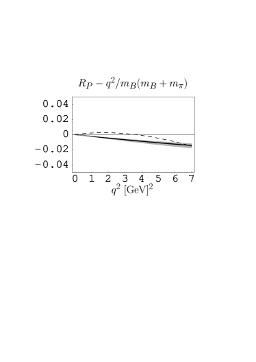
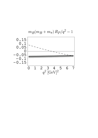
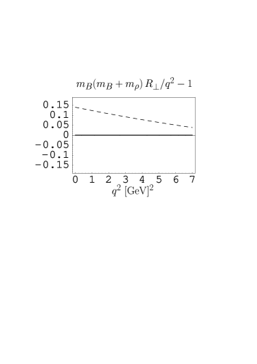
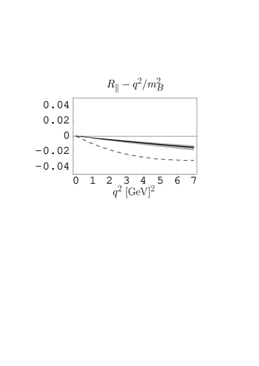
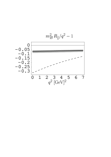
Figure 4: Illustration of the relations (146) for $B\to\pi$ and $B\to\rho$ form factors. On the left-hand side we plot the ratios $R_{P,\perp,\parallel}$ minus the corresponding values in the symmetry limit. The right-hand side shows $R_{P,\perp,\parallel}$ divided by their symmetry limits minus 1. The dashed line corresponds to the form factors predicted from QCD light-cone sum rules in [29, 30]. The solid line is the order $\lambda^{0}$ result supplemented by $\alpha_{s}$ corrections as calculated in [9]. The tensor form factors are evaluated at the scale $m$. The grey error band reflects the theoretical uncertainty from varying the scale of $\alpha_{s}$ from $m/2$ to $2m$.

A subtle question concerns the power-counting of hadronic matrix elements in soft-collinear effective theory. In contrast to the well-known Isgur-Wise form factor in HQET [31], which is constrained to scale as $\lambda^{0}$ by its normalization at zero recoil, the power counting for the universal form factors $\xi_{i}^{(0)}(E)$ is not determined by the effective theory. The scaling behaviour of the quark fields and of the meson states with $\lambda$ is not sufficient to determine the corresponding scaling behaviour of form factors. Formally, we have from the normalization of hadronic states

$$\langle P(p^{\prime})|\sim\lambda^{-2},\qquad|B(m_{B}v)\rangle\sim\lambda^{-3},$$ (148)

where we used $p^{\prime}\approx En_{-}$. Together with $\xi\sim\lambda$ and $h_{v}\sim\lambda^{3}$ this results in

$$\langle P(p^{\prime})|\xi\,\Gamma\,W_{c}\,h_{v}|B(m_{B}v)\rangle \sim \lambda^{-1}\,X(\lambda).$$ (149)

Here we introduced the function $X(\lambda)$ which parameterizes the probability to find the parton configuration corresponding to the current operator in the incoming and outgoing meson states. While the probability to find a nearly on-shell $b$-quark in a $B$ meson is of order one, the configuration with one collinear quark (jet) carrying most of the light meson’s energy is expected to be suppressed. The suppression factor is usually estimated from the end-point behaviour of the meson’s two-particle light cone distribution amplitude (see [9] and references therein), which gives

$$\left\{\xi_{P}^{(0)}(E)\,,\ \xi_{\perp}^{(0)}(E)\,,\ (v\cdot\epsilon)~{}\xi_{\parallel}^{(0)}(E)\right\}\ \propto\ \lambda^{3}\ .$$ (150)

From this one concludes that $X(\lambda)\sim\lambda^{4}$. In our discussion of power corrections to the transition form factors we implicitly assumed that the matrix elements of higher-order terms in the effective current have the same $\lambda^{4}$ suppression as the leading-order matrix element. There might be further dynamical suppression of the higher-order matrix elements, but an understanding of this requires knowledge of the meson wavefunctions that is not provided by the effective theory.

In this respect soft-collinear effective theory applied to heavy-to-light decays at large recoil is rather different from HQET for $B\to D^{(*)}$ form factors. In the latter case one obtains non-trivial form factors relations beyond leading order in $\lambda$, because the heavy-quark flavour symmetry also relates the initial and final hadronic states. (The same symmetry is responsible for the absolute normalization of the Isgur-Wise form factors at zero recoil.) An analogous symmetry that relates light meson states is absent in soft-collinear effective theory.

6 Conclusions

The effective field theory approach to soft-collinear factorization initiated by [2, 4] provides a new framework for formulating the factorization theorems of QCD for processes with energetic, nearly massless particles. Beyond this it opens up the possibility to investigate power corrections to such processes more systematically than in the diagrammatic framework. In this paper we have taken a first step in this direction by deriving the effective Lagrangian to second order in the expansion parameter $\lambda$, and the corresponding power corrections to weak interaction quark currents that convert a heavy quark into energetic light partons.

We have formulated the effective theory in a position space representation rather than the less familiar hybrid position-momentum space representation adopted in [2]. Although the physical content of the two formulations should be identical, the choice of representation implies significant technical differences. In the hybrid representation the rapid variations of collinear fields are extracted and become field momentum labels, such that a collinear field $\xi_{p}(x)$ has only a residual ultrasoft spatial variation. In position space collinear fields $\xi(x)$ are characterized by their most rapid spatial variation in every direction with no possibility to extract superimposed slow variations. In this formulation the multipole expansion of the argument of ultrasoft fields accomplishes the equivalent of extracting the ultrasoft variation of collinear fields in the hybrid representation. A consequence of this is that the gauge symmetry of QCD is implemented differently in the two formulations of soft-collinear effective theory.

The main results of this paper can be summarized as follows:

• We have derived the soft-collinear effective Lagrangian to order $\lambda^{2}$ including ultrasoft quark fields. We have also found that the tree-level Lagrangian is exact, since Lorentz invariance protects every operator (at any order in $\lambda$) from acquiring a non-trivial coefficient function.

• We have derived the effective heavy-to-light current relevant for exclusive $B$ meson decays to order $\lambda^{2}$ and investigated its properties under reparameterizations of the arbitrary vectors that define the momentum decomposition in the effective theory. An expression for the current at order $\lambda$ has been previously given in [20]. We differ from this result by an additional term that comes from the coupling of transverse collinear gluons to the heavy quark.

We then investigated whether relations between the transition form factors for $B$ meson decay into a light pseudoscalar or vector meson survive when one includes power corrections. Including terms of order $\lambda$ we find one relation among the three form factors for decays into pseudoscalar mesons and two relations among the seven form factors for decays into vector mesons. Including terms of order $\lambda^{2}$ no relations survive. This is to be compared to the existence of two (five) form factor relations for pseudoscalar (vector) mesons in the infinite quark mass limit.

Note added in proof.

In the revised version of [23] (hep-ph/0205289v2) Bauer, Pirjol and Stewart have also given the tree-level matching coefficient of the operator $J_{1}$, which appears in the expansion of the heavy-light current at order $\lambda$, see (123). Their result agrees with ours.

Appendix A Derivation of equations (63) and (64)

In this appendix we provide the details of the manipulations that lead to the final form of the second-order Lagrangian, (63) and (64), for abelian gauge fields. We start from (56) and the explicit expressions for the various terms given below (56).

To obtain (62) we use the equation of motion first for $\xi$, then for $\bar{\xi}$. We have to keep the order $\lambda$ terms in the equation of motion and account for the fact that the Lagrangian changes after the first use of the equation of motion. After performing the steps that lead to (62) one has to add to (57), (58) the terms

$$\Delta{\cal L}_{\xi}^{(2)} = \bar{\xi}\,(gx_{\perp}A_{\rm us})\left(in_{-}D+iD\hskip-5.89996pt/_{\perp c}\frac{1}{in_{+}D_{c}}iD\hskip-5.89996pt/_{\perp c}\right)(gx_{\perp}A_{\rm us})\,\frac{n\hskip-4.49997pt/_{+}}{2}\,\xi$$

$$+\,\bar{\xi}\left[iD\hskip-5.89996pt/_{\perp c}\frac{1}{in_{+}D_{c}}\,gA\hskip-5.89996pt/_{\perp\rm us}+gA\hskip-5.89996pt/_{\perp\rm us}\frac{1}{in_{+}D_{c}}\,iD\hskip-5.89996pt/_{\perp c},\,igx_{\perp}A_{\rm us}\right]\frac{n\hskip-4.49997pt/_{+}}{2}\,\xi,$$

$$\Delta{\cal L}_{\xi q}^{(2)} = -\,\bar{\xi}\,(igx_{\perp}A_{\rm us})\,iD\hskip-5.89996pt/_{\perp c}W_{c}\,q+\mbox{ ``h.c.''}$$ (151)

from the equation of motion. Formally, using the equations of motion in (61) is equivalent to the change of variables $\xi\to(1+igx_{\perp}A_{\rm us})\,\xi$ in ${\cal L}_{\xi}^{(0)}$ and ${\cal L}_{\xi}^{(1)}$.

The terms in $\Delta{\cal L}_{\xi}^{(2)}$ can be simplified by using the identities (valid only for abelian gauge fields)

$$(x_{\perp}A_{\rm us})\,(in_{-}D)\,(x_{\perp}A_{\rm us})=\frac{1}{2}\left\{(in_{-}D),\,(x_{\perp}A_{\rm us})^{2}\right\},$$

$$(x_{\perp}A_{\rm us})\,iD\hskip-5.89996pt/_{\perp c}\frac{1}{in_{+}D_{c}}iD\hskip-5.89996pt/_{\perp c}\,(x_{\perp}A_{\rm us})$$ (152)

$$\qquad=\frac{1}{2}\left\{iD\hskip-5.89996pt/_{\perp c}\frac{1}{in_{+}D_{c}}iD\hskip-5.89996pt/_{\perp c},\,(x_{\perp}A_{\rm us})^{2}\right\}+A\hskip-5.89996pt/_{\perp\rm us}\,\frac{1}{in_{+}D_{c}}\,A\hskip-5.89996pt/_{\perp\rm us},$$

$$\left[iD\hskip-5.89996pt/_{\perp c}\,\frac{1}{in_{+}D_{c}}\,A\hskip-5.89996pt/_{\rm us},\,(ix_{\perp}A_{\rm us})\right]$$ (153)

$$\qquad=\left[A\hskip-5.89996pt/_{\perp\rm us}\,\frac{1}{in_{+}D_{c}}\,iD\hskip-5.89996pt/_{\perp c},\,(ix_{\perp}A_{\rm us})\right]=-A\hskip-5.89996pt/_{\perp\rm us}\,\frac{1}{in_{+}D_{c}}\,A\hskip-5.89996pt/_{\perp\rm us}.$$ (154)

Using again the leading order equations of motion for $\xi$ and $\bar{\xi}$, one obtains

$$\Delta{\cal L}_{\xi}^{(2)}=-\,\bar{\xi}\,gA\hskip-5.89996pt/_{\perp\rm us}\,\frac{1}{in_{+}D_{c}}\,gA\hskip-5.89996pt/_{\perp\rm us}\,\frac{n\hskip-4.49997pt/_{+}}{2}\,\xi,$$ (155)

which exactly cancels the corresponding term in (57). The remaining terms in ${\cal L}_{\xi}^{(2)}$ can be simplified by commutator relations and the equation of motion. The identity

$$\frac{1}{(in_{+}D_{c})^{2}}=i\left[\frac{1}{in_{+}D_{c}},\,\frac{1}{2}\,n_{-}x\right]$$ (156)

allows us to write

$$\bar{\xi}\,iD\hskip-5.89996pt/_{\perp c}\,\frac{1}{in_{+}D_{\rm c}}\,(gn_{+}A_{\rm us})\,\frac{1}{in_{+}D_{c}}\,iD\hskip-5.89996pt/_{\perp c}\,\frac{n\hskip-4.49997pt/_{+}}{2}\,\xi=\frac{1}{2}\,\bar{\xi}\,(n_{-}x)\left[(n_{-}\partial)\,(gn_{+}A_{\rm us})\right]\frac{n\hskip-4.49997pt/_{+}}{2}\xi.$$ (157)

This term combines with the first term in the third line of (57) into $n_{+}^{\mu}n_{-}^{\nu}F_{\mu\nu}^{\rm us}$. Then we use

$$2\left(\left[(x_{\perp}\partial)\,A\hskip-5.89996pt/_{\perp\rm us}\right]\,\frac{1}{in_{+}D_{c}}\,iD\hskip-5.89996pt/_{\perp c}+iD\hskip-5.89996pt/_{\perp c}\,\frac{1}{in_{+}D_{c}}\,\left[(x_{\perp}\partial)\,A\hskip-5.89996pt/_{\perp\rm us}\right]\right)=$$ (158)

$$i\left[x_{\perp}^{\mu}x_{\perp}^{\nu}[\partial_{\nu}A_{\mu,\rm us}],\,iD\hskip-5.89996pt/_{\perp c}\,\frac{1}{in_{+}D_{c}}\,iD\hskip-5.89996pt/_{\perp c}\right]+\left(x_{\perp}^{\mu}\gamma_{\perp}^{\nu}F_{\mu\nu}^{\rm us}\,\frac{1}{in_{+}D_{c}}\,iD\hskip-5.89996pt/_{\perp c}+iD\hskip-5.89996pt/_{\perp c}\,\frac{1}{in_{+}D_{c}}\,x_{\perp}^{\mu}\gamma_{\perp}^{\nu}F_{\mu\nu}^{\rm us}\right)$$

to rewrite the second line of (57):

$$\bar{\xi}\left(iD\hskip-5.89996pt/_{\perp c}\frac{1}{in_{+}D_{c}}\,\left[(x_{\perp}\partial)\,gA\hskip-5.89996pt/_{\perp\rm us}\right]+\left[(x_{\perp}\partial)\,gA\hskip-5.89996pt/_{\perp\rm us}\right]\,\frac{1}{in_{+}D_{c}}\,iD\hskip-5.89996pt/_{\perp c}\right)\frac{n\hskip-4.49997pt/_{+}}{2}\xi=$$

$$\hskip 56.9055pt\frac{1}{2}\,\bar{\xi}\left(iD\hskip-5.89996pt/_{\perp c}\,\frac{1}{in_{+}D_{c}}\,x_{\perp}^{\mu}\gamma_{\perp}^{\nu}\,gF_{\mu\nu}^{\rm us}+x_{\perp}^{\mu}\gamma_{\perp}^{\nu}\,gF_{\mu\nu}^{\rm us}\,\frac{1}{in_{+}D_{c}}\,iD\hskip-5.89996pt/_{\perp c}\right)\frac{n\hskip-4.49997pt/_{+}}{2}\,\xi$$

$$\hskip 56.9055pt-\,\frac{1}{2}\,\bar{\xi}\left\{x_{\perp}^{\mu}\left[(x_{\perp}\partial)\,(n_{-}\partial)\,A_{\mu,\rm us}\right]\right\}\frac{n\hskip-4.49997pt/_{+}}{2}\,\xi.$$ (159)

With this all remaining terms involving ultrasoft gauge fields can again be expressed in terms of field strength tensors and (63) follows. The derivation of (64), where one has to take account of (151), is straightforward. The application of the $\xi$ equation of motion at several steps in this calculation is equivalent to the field redefinition (65).

Appendix B Heavy-to-light form factors

The form factors relevant to heavy-to-light $B$ decays are defined as in [9]

$$\langle P(p^{\prime})|\bar{\psi}\,\gamma^{\mu}b|\bar{B}(p)\rangle=f_{+}(q^{2})\left[p^{\mu}+p^{\prime\,\mu}-\frac{m_{B}^{2}-m_{P}^{2}}{q^{2}}\,q^{\mu}\right]+f_{0}(q^{2})\,\frac{m_{B}^{2}-m_{P}^{2}}{q^{2}}\,q^{\mu},$$ (160)

$$\langle P(p^{\prime})|\bar{\psi}\,\sigma^{\mu\nu}q_{\nu}b|\bar{B}(p)\rangle=\frac{if_{T}(q^{2})}{m_{B}+m_{P}}\left[q^{2}(p^{\mu}+p^{\prime\,\mu})-(m_{B}^{2}-m_{P}^{2})\,q^{\mu}\right],$$ (161)

where $m_{B}$ is the $B$ meson mass, $m_{P}$ the mass of the pseudoscalar meson and $q=p-p^{\prime}$. The relevant form factors for $B$ decays into vector mesons are defined as

$$\langle V(p^{\prime},\varepsilon^{\ast})|\bar{\psi}\gamma^{\mu}b|\bar{B}(p)\rangle=\frac{2iV(q^{2})}{m_{B}+m_{V}}\,\epsilon^{\mu\nu\rho\sigma}\varepsilon^{\ast}_{\nu}\,p^{\prime}_{\rho}p_{\sigma},$$ (162)

$$\langle V(p^{\prime},\varepsilon^{\ast})|\bar{\psi}\gamma^{\mu}\gamma_{5}b|\bar{B}(p)\rangle = 2m_{V}A_{0}(q^{2})\,\frac{\varepsilon^{\ast}\cdot q}{q^{2}}\,q^{\mu}+(m_{B}+m_{V})\,A_{1}(q^{2})\left[\varepsilon^{\ast\mu}-\frac{\varepsilon^{\ast}\cdot q}{q^{2}}\,q^{\mu}\right]$$ (163)

$$-\,A_{2}(q^{2})\,\frac{\varepsilon^{\ast}\cdot q}{m_{B}+m_{V}}\left[p^{\mu}+p^{\prime\,\mu}-\frac{m_{B}^{2}-m_{V}^{2}}{q^{2}}\,q^{\mu}\right],$$

$$\langle V(p^{\prime},\varepsilon^{\ast})|\bar{\psi}\sigma^{\mu\nu}q_{\nu}b|\bar{B}(p)\rangle=2\,T_{1}(q^{2})\,\epsilon^{\mu\nu\rho\sigma}\varepsilon^{\ast}_{\nu}\,p_{\rho}p^{\prime}_{\sigma},$$ (164)

$$\langle V(p^{\prime},\varepsilon^{\ast})|\bar{\psi}\sigma^{\mu\nu}\gamma_{5}q_{\nu}b|\bar{B}(p)\rangle = (-i)\,T_{2}(q^{2})\left[(m_{B}^{2}-m_{V}^{2})\,\varepsilon^{\ast\mu}-(\varepsilon^{\ast}\cdot q)\,(p^{\mu}+p^{\prime\,\mu})\right]$$ (165)

$$+\,(-i)\,T_{3}(q^{2})\,(\varepsilon^{\ast}\cdot q)\left[q^{\mu}-\frac{q^{2}}{m_{B}^{2}-m_{V}^{2}}(p^{\mu}+p^{\prime\,\mu})\right],$$

where $m_{V}$ ($\varepsilon$) is the mass (polarization vector) of the vector meson and we use the sign convention $\epsilon^{0123}=-1$.

Calculating the various traces in (140) we can express the form factors (160) to (165) in terms of the sets $f_{P}^{(kl)}$ and $f_{\perp}^{(kl)}$, $f_{\parallel}^{(kl)}$ introduced in (141). Neglecting terms suppressed by a relative factor $m_{P,V}^{2}/E^{2}\sim\lambda^{4}$ we obtain

$$f_{+}(q^{2}) = f_{P}^{(++)}(E)-f_{P}^{(+-)}(E)-\frac{q^{2}}{m_{B}^{2}}\left(f_{P}^{(-+)}(E)-f_{P}^{(--)}(E)\right),$$

$$f_{0}(q^{2}) = \frac{m_{B}^{2}-q^{2}}{m_{B}^{2}}\left\{f_{P}^{(++)}(E)-f_{P}^{(+-)}(E)+\frac{q^{2}}{m_{B}^{2}}\left(f_{P}^{(-+)}(E)-f_{P}^{(--)}(E)\right)\right\},$$

$$f_{T}(q^{2}) = \frac{m_{B}+m_{P}}{m_{B}}\left\{f_{P}^{(++)}(E)+f_{P}^{(+-)}(E)-f_{P}^{(-+)}(E)-f_{P}^{(--)}(E)\right\}$$ (166)

for decays into light pseudoscalars, and

$$V(q^{2}) = \frac{m_{B}+m_{V}}{m_{B}}\left\{f_{\perp}^{(++)}(E)+f_{\perp}^{(+-)}(E)-f_{\perp}^{(-+)}(E)-f_{\perp}^{(--)}(E)\right\},$$

$$A_{0}(q^{2}) = \frac{m_{B}^{2}-q^{2}}{2m_{B}m_{V}}\left\{f_{\parallel}^{(++)}(E)-f_{\parallel}^{(+-)}(E)+\frac{q^{2}}{m_{B}^{2}}\left(f_{\parallel}^{(-+)}(E)-f_{\parallel}^{(--)}(E)\right)\right\},$$

$$A_{1}(q^{2}) = \frac{m_{B}^{2}-q^{2}}{m_{B}(m_{B}+m_{V})}\left\{f_{\perp}^{(++)}(E)+f_{\perp}^{(+-)}(E)+f_{\perp}^{(-+)}(E)+f_{\perp}^{(--)}(E)\right\},$$

$$A_{2}(q^{2}) = -\frac{m_{B}+m_{V}}{m_{B}}\left\{f_{\parallel}^{(++)}(E)-f_{\parallel}^{(+-)}(E)-\frac{q^{2}}{m_{B}^{2}}\left(f_{\parallel}^{(-+)}(E)-f_{\parallel}^{(--)}(E)\right)\right\}$$

$$+\frac{m_{B}+m_{V}}{m_{B}}\left\{f_{\perp}^{(++)}(E)+f_{\perp}^{(+-)}(E)+f_{\perp}^{(-+)}(E)+f_{\perp}^{(--)}(E)\right\},$$

$$T_{1}(q^{2}) = f_{\perp}^{(++)}(E)-f_{\perp}^{(+-)}(E)-\frac{q^{2}}{m_{B}^{2}}\left(f_{\perp}^{(-+)}(E)-f_{\perp}^{(--)}(E)\right),$$

$$T_{2}(q^{2}) = \frac{m_{B}^{2}-q^{2}}{m_{B}^{2}}\left\{f_{\perp}^{(++)}(E)-f_{\perp}^{(+-)}(E)+\frac{q^{2}}{m_{B}^{2}}\left(f_{\perp}^{(-+)}(E)-f_{\perp}^{(--)}(E)\right)\right\},$$

$$T_{3}(q^{2}) = -f_{\parallel}^{(++)}(E)-f_{\parallel}^{(+-)}(E)+f_{\parallel}^{(-+)}(E)+f_{\parallel}^{(--)}(E)$$ (168)

$$+f_{\perp}^{(++)}(E)-f_{\perp}^{(+-)}(E)+\frac{q^{2}}{m_{B}^{2}}\left(f_{\perp}^{(-+)}(E)-f_{\perp}^{(--)}(E)\right)$$

for decays into light vector mesons.

References

- [1] C. W. Bauer, S. Fleming and M. E. Luke, Phys. Rev. D63 (2001) 014006 [hep-ph/0005275].
- [2] C. W. Bauer, S. Fleming, D. Pirjol, and I. W. Stewart, Phys. Rev. D63 (2001) 114020 [hep-ph/0011336].
- [3] C. W. Bauer and I. W. Stewart, Phys. Lett. B516 (2001) 134 [hep-ph/0107001].
- [4] C. W. Bauer, D. Pirjol, and I. W. Stewart, Phys. Rev. D65 (2002) 054022 [hep-ph/0109045].
- [5] C. W. Bauer, S. Fleming, D. Pirjol, I. Z. Rothstein, and I. W. Stewart, Phys. Rev. D66 (2002) 014017 [hep-ph/0202088].
- [6] J. C. Collins, D. E. Soper, and G. Sterman, in: Perturbative Quantum Chromodynamics, ed. A. H. Mueller (World Scientific, Singapore, 1989), p. 1.
- [7] S. J. Brodsky and G. P. Lepage, in: Perturbative Quantum Chromodynamics, ed. A. H. Mueller (World Scientific, Singapore, 1989), p. 93.
- [8] M. Beneke, Phys. Rept. 317 (1999) 1 [hep-ph/9807443].
- [9] M. Beneke and T. Feldmann, Nucl. Phys. B592 (2001) 3 [hep-ph/0008255].
- [10] M. Beneke and V. A. Smirnov, Nucl. Phys. B522 (1998) 321 [hep-ph/9711391].
- [11] J. B. Kogut and D. E. Soper, Phys. Rev. D1 (1970) 2901.
- [12] S. J. Brodsky, H.-C. Pauli, and S. S. Pinsky, Phys. Rept. 301 (1998) 299 [hep-ph/9705477].
- [13] P. P. Srivastava and S. J. Brodsky, Phys. Rev. D61 (2000) 025013 [hep-ph/9906423].
- [14] A. V. Manohar, T. Mehen, D. Pirjol, and I. W. Stewart, Phys. Lett. B539 (2002) 59 [hep-ph/0204229].
- [15] A. V. Manohar, Phys. Rev. D56 (1997) 230 [hep-ph/9701294].
- [16] E. Eichten and B. Hill, Phys. Lett. B234 (1990) 511.
- [17] H. Georgi, Phys. Lett. B240 (1990) 447.
- [18] B. Grinstein, Nucl. Phys. B339 (1990) 253.
- [19] S. Coleman and R. Norton, Nuov. Cim. 38 (1965) 438.
- [20] J. Chay and C. Kim, Phys. Rev. D65 (2002) 114016 [hep-ph/0201197].
- [21] J. Chay and C. Kim, [hep-ph/0205117].
- [22] M. E. Luke and A. V. Manohar, Phys. Lett. B286 (1992) 348 [hep-ph/9205228].
- [23] C. W. Bauer, D. Pirjol and I. W. Stewart, [hep-ph/0205289].
- [24] M. Beneke, G. Buchalla, M. Neubert, and C. T. Sachrajda, Phys. Rev. Lett. 83 (1999) 1914 [hep-ph/9905312].
- [25] M. Beneke, T. Feldmann, and D. Seidel, Nucl. Phys. B612 (2001) 25 [hep-ph/0106067].
- [26] S. W. Bosch and G. Buchalla, Nucl. Phys. B621 (2002) 459 [hep-ph/0106081].
- [27] J. Charles, A. Le Yaouanc, L. Oliver, O. Pene, and J. C. Raynal, Phys. Rev. D60 (1999) 014001 [hep-ph/9812358].
- [28] G. Burdman and G. Hiller, Phys. Rev. D63 (2001) 113008 [hep-ph/0011266].
- [29] P. Ball, JHEP 09 (1998) 005 [hep-ph/9802394].
- [30] P. Ball and V. M. Braun, Phys. Rev. D58 (1998) 094016 [hep-ph/9805422].
- [31] N. Isgur and M. B. Wise, Phys. Lett. B237 (1990) 527.