IFT/02/17

June 2002

Racetrack models in theories from extra dimensions

Rafał Ciesielski and Zygmunt Lalak

Institute of Theoretical Physics

University of Warsaw, Poland

Abstract

We have investigated moduli stabilization leading to hierarchical supersymmetry breakdown in racetrack models with two moduli fields simultaneously present in the effective racetrack superpotential. We have shown that stabilization of moduli occurs when a shift symmetry of the moduli space becomes gauged. This gauging results in a $D$-term contribution to the scalar potential that depends on moduli scalars. To break supersymmetry at a minimum created this way in the case where only a single combination of moduli is present in the superpotential one needs supergravity corrections. If the superpotential depends on two independent combinations of moduli, supersymmetry is broken by non-vanishing $F$-terms without supergravity terms. Some of the minima that we see correspond to a non-vanishing expectation value of the blowing-up modulus in the case of type IIB orientifold models. We point out that the mass of the gauge boson associated with gauged shift symmetry becomes naturally light in warped compactifications.

June 2002

1 Introduction

Supersymmetry provides a technically natural and rich in physical implications method of controlling the hierarchy of mass scales in four-dimensional field theories, to all orders in perturbative calculations. However, supersymmetry must be broken at low energies to account properly for observable phenomenology. The most economic way of doing this is to couple the gauge and matter Lagrangian to gravity in the locally supersymmetric manner and to break local supersymmetry spontaneously. First, one avoids the appearance of the massless fermion – the Goldstino becomes the spin $1/2$- component of the massive gravitino. Second, weak gravitational couplings account for the natural suppression of the communication of the effects of the supersymmetry breakdown to the observable sector. In the flat limit this procedure gives rise to the Lagrangian with explicitly but softly broken global supersymmetry. On the other hand in theories borne in higher dimensions there exist naturally light fields, which are neutral under gauge interactions and form flat or run-away directions in the field space. Such moduli fields arise very naturally in theories with extra dimensions as extra-components of the higher-dimensional metric tensor, form fields and gravitini. After compactification such fields may contribute to the four-dimensional cosmological constant, through their potentials and transverse gradients. Hence, what one really requires from the successful scenario of supersymmetry breakdown is not only generation of 1 TeV mass splittings in observable supermultiplets, but also stabilization of moduli while achieving a nearly vanishing four-dimensional cosmological constant.

Among various proposals heading in this direction a particularly simple one is the idea of using several gaugino condensates, i.e. the racetrack models [1],[2],[3]. Technically it reduces down to generating a superpotential containing several components that depend exponentially on moduli scalars. As demonstrated over the years such exponential contributions may arise not only from strongly interacting gauge sectors, but also from nontrivial warp factors along transverse dimensions or/and brane solutions of higher dimensional supergravity and string theories. Another ingredient coming from type I and type II orientifold theories are additional, twisted, moduli [4]. These moduli enter, along the untwisted dilaton (and sometimes radion) the kinetic functions of some nonabelian gauge groups. Further to this, in type II B orientifold models there appear anomalous $U(1)$ gauge factors, whose effective Fayet-Iliopoulos terms are proportional to the background values of the twisted moduli. Hence, these moduli obtain an additional contribution to their potential through the anomalous D-terms. The presence of the radion in the gauge kinetic functions has been found long ago in the case of weakly coupled heterotic superstring [5],[6], then in the case of the strongly coupled heterotic superstring [7], and recently in warped five-dimensional brane models [8].

In what follows we shall investigate to what extent one can achieve successful supersymmetry breakdown and moduli stabilization with the use of the generalized racetrack models in four-dimensional supergravities enhanced by the extra-dimensional features discussed above.

2 Moduli dependent Fayet-Iliopoulos terms

First, let us summarize briefly the features of the four-dimensional models with field-dependent FI terms that are relevant for this note. Basically, such terms can be understood as D-terms arising upon gauging of global translations along direction of certain moduli fields. Let us call a representative modulus $Z$, and assume that its Kähler function depends only on $Z+\bar{Z}$, $K=K(Z+\bar{Z})$. Then the shift $Z\rightarrow Z-i\delta/2\,\Lambda$ is the isometry of the associated Kähler manifold generated by the Killing vector $X=-i\delta/2$. To gauge this isometry we introduce in the supersymmetric way the massless vector field $A_{\mu}$ which enters the covariant derivative $D_{\mu}=\partial_{\mu}+ig\delta/2A_{\mu}$, where $g$ is the gauge coupling constant. Due to supersymmetry there appears the prepotential $D$, fulfilling the Killing equation $K_{{Z}\bar{{Z}}}\bar{X}=i\partial D/\partial{Z}$. This prepotential generates the scalar potential for ${Z}$, $V=\frac{1}{2}g^{2}D^{2}$, and plays the role of the field dependent Fayet-Iliopoulos term $\xi^{2}$, $\xi^{2}=D$. It is easy to see that, up to a constant, the $D$/FI term associated with the Killing vector $X$ is $D=\delta/2\partial K/\partial\bar{{Z}}$. In addition, the covariantized kinetic term for the scalar ${Z}$ gives rise to the mass term for the vector boson,

$$m_{A}^{2}=\frac{M_{P}^{2}g^{2}\delta^{2}}{2}K_{{Z}\bar{{Z}}},$$ (1)

where we have put explicitly the 4d Planck scale. In general, when the gauge coupling $g$ is field dependent, $g=g(z)$, the local shift of ${Z}$ is anomalous, and one needs to introduce other fields charged under the gauge symmetry to cancel the anomaly. This issue has been discussed at length in a number of papers and in what follows we assume that such a compensation is possible whenever we need it (but see [9],[10]). The well known case of a field-dependent D-term is the one of the heterotic string, where one gauges the imaginary shift of the dilaton. There $K=-\log(S+\bar{S})$, $D=(M_{P}^{2}\delta)/(2(S+\bar{S}))$, and the mass of the gauge boson is naturally of the order of the Planck scale. The case of type IIB orientifolds corresponds to $K=\frac{1}{2}(M+\bar{M})^{2}$ (see [11] and references therein). This gives $D=\delta/2(M+\bar{M})$. An interesting possibility is offered by warped compactifications [8],[12]. There $K=-3\log(f(T+\bar{T}))$, where the function $f$ reflects the vacuum configuration of the warp factor along the extra-dimensions. To be specific let us take the case of the Randall-Sundrum model, $f=\beta(1-e^{-(T+\bar{T})})$. This results in the Fayet-Iliopoulos term

$$D=-\frac{\delta}{2}M_{P}^{2}\frac{e^{-(T+\bar{T})}}{1-e^{-(T+\bar{T})}},$$ (2)

and the mass of the gauge boson is

$$m_{A}^{2}=\frac{3g^{2}\delta^{2}}{2}M_{P}^{2}\frac{e^{-(T+\bar{T})}}{1-e^{-(T+\bar{T})}}.$$ (3)

In the case of the Randall-Sundrum model the warp factor can easily be taken in such a way, that the mass scale one the warped brane, $e^{-(T+\bar{T})}M_{P}^{2}$ becomes $(1\;{\rm TeV})^{2}$. Then of course the mass of the gauge boson, and the field dependent FI term are also of the order $(1\;{\rm TeV})^{2}$. Hence, in the warped case the gauge boson associated with the ‘anomalous’ $U(1)$ group may be naturally light. Of course the microscopic picture is likely to somewhat more complicated, as for instance one expect generation of the moduli dependent superpotential in the warped models, which may break the imaginary shift symmetry.

3 Moduli stabilization

In what follows we shall concentrate on a model resemblig the structure of models derived from type IIB orientifolds, with two types of moduli: the dilaton $S$ and the analog of a twisted modulus $M$. We shall assume two $SU(N_{i}),\;i=1,2$ gauge group with gauge dependent kinetic functions $f_{i}=S+c_{i}M$. Condensation of the gaugini of the two $SU(N)$s give rise to the exponential superpotential for the moduli:

$$W(S,M) = {M_{P}}^{3}\Bigg{(}\alpha e^{\frac{-24\pi^{2}}{b_{1}}\Big{(}\frac{S+{c_{1}}M}{{M_{P}}}\Big{)}}+\beta e^{\frac{-24\pi^{2}}{b_{2}}\Big{(}\frac{S+{c_{2}}M}{{M_{P}}}\Big{)}}\Bigg{)}$$ (4)

where the $b_{i}$ are one-loop beta function coefficients normalized through $\;\beta(g_{i})=-\frac{b_{i}}{(4\pi)^{2}}g_{i}^{3}\;\;$,
and $\alpha$, $\beta$ are model dependent parameters.

We are interested in the question of stabilization of moduli and hierarchical supersymmetry breaking in such a setup, in the cases of globally and locally supersymmetric models. In fact, it would be natural to start with a single exponential term in the superpotential, and to play with possible variation of the Kähler function to stabilize the moduli. However, within the restricted class of Kähler potentials we consider we were unable to find a minimum of the potential neither in the globally supersymmetric nor in the supergravity version of the model. Moreover, it turns out to be difficult to find a minimum of the potential even with two exponential terms (‘two condensates’). That this would be the case one could foresee on the basis of the negative result in the case $c_{1}=-c_{2}$ considered in [14] in the context of the Horava-Witten model [15]. The strategy of the search for reasonable minima with hierarchical susy breaking is analogous to that of [14]: first we try to find minima (with unbroken susy) of the globally supersymmetric Lagrangian, and then we switch on gravity-induced corrections. In addition, we shall check the sensitivity of the minimization with respect to a deformation of the Kähler function for the $M$-modulus, and we shall switch on the $M$-dependent Fayet-Iliopoulos term.

We start with the case that can be followed analytically. The first simplifying assumption is that the kinetic functions are the same, $f_{1}=f_{2}$. This means that ${c_{1}}={c_{2}}=c$. Then we perform a holomorphic redefinition of variables $S,\;M$:

$$f_{1}=f_{2}=S+{c}M\equiv{Z}.$$ (5)

In new variables the Kähler potential takes the form

$${K}({S},\bar{{S}},{Z},\bar{{Z}}) = -\ln({S}+\bar{{S}})+\frac{1}{2{c}^{2}}({Z}+\bar{{Z}}-S-\bar{S})^{2}+\frac{\gamma}{4{c}^{4}}({Z}+\bar{{Z}}-S-\bar{S})^{4},$$

where $\gamma$ is a new, presumably small, real parameter measuring the departure from the quadratic Kähler potential for $M$. The superpotential becomes

$$W({Z}) = \alpha e^{-\frac{{Z}}{{\widetilde{b_{1}}}}}+\beta e^{-\frac{{Z}}{{\widetilde{b_{2}}}}}$$ (8)

where $\widetilde{b_{i}}=\frac{b_{i}}{24\pi^{2}}$, and the inverse Kähler metric is

$$g^{i\bar{j}}=({S}+\bar{{S}})^{2}\left(\begin{array}[]{cc}\frac{1}{({S}+\bar{{S}})^{2}}\frac{{c}^{4}}{{c}^{2}+3\gamma({Z}+\bar{{Z}}-{S}-\bar{{S}})^{2}}+1&1\\ 1&1\\ \end{array}\right).$$ (9)

The scalar potential contains, in the global limit,

$$V({S},\bar{{S}},{Z},\bar{{Z}})=g^{{Z}\bar{{Z}}}\Big{|}\frac{\partial W({Z})}{\partial{Z}}\Big{|}^{2}+\frac{1}{2}g^{2}D^{2},$$ (10)

where $D$ is the $U(1)$ $D$-term

$$D=\frac{1}{2c^{2}}({Z}+\bar{{Z}}-{S}-\bar{{S}}+\frac{\gamma}{c^{2}}({Z}+\bar{{Z}}-{S}-\bar{{S}})^{3}).$$ (11)

The scalar potential of the model in new variables $Z,\;S$ before gauging the imaginary translation takes the form

$$V({S},\bar{{S}},{Z},\bar{{Z}})=\bigg{(}\frac{{c}^{4}}{{c}^{2}+3\gamma({Z}+\bar{{Z}}-{S}-\bar{{S}})^{2}}+({S}+\bar{{S}})^{2}\bigg{)}\Big{|}\frac{\partial W({Z})}{\partial{Z}}\Big{|}^{2}.$$ (12)

This potential has a flat direction, which is located along $S$ for $Z$ fulfilling the condition for unbroken global supersymmetry $\partial W/\partial Z=0$:

$$\frac{\partial W({Z})}{\partial{Z}}=0 \Rightarrow {Z}_{0}=\frac{{\widetilde{b_{1}}}{\widetilde{b_{2}}}}{{\widetilde{b_{2}}}-{\widetilde{b_{1}}}}\ln\bigg{(}-\frac{\beta{\widetilde{b_{1}}}}{\alpha{\widetilde{b_{2}}}}\bigg{)}.$$ (13)

Putting in the nonzero coefficient $\gamma$ of the quartic term in the Kähler potential doesn’t change the situation.

However, switching on the field-dependent Fayet-Iliopoulos term makes a difference. To simplify the reasoning and to make it somewhat model-independent let us replace the original superpotential by its expansion around the point $Z_{0}$ such that $\partial W/\partial Z|_{Z_{0}}=0$

$$W({Z})=w+({Z}-{Z}_{0})^{2}w_{2}$$ (14)

where $w=W({Z}_{0})$ , and $w_{2}=\frac{\partial^{2}W({Z})}{\partial{Z}^{2}}|_{{Z}_{0}}$. One readily finds a minimum at the point $S={Z}_{0}$ and ${Z}={Z}_{0}$. Hence the D-term contribution to the potential localizes $S$ with respect to $Z$, which in turns gets localized by the superpotential.

In the presence of the nonzero FI term there exists a minimum of the potential for any real $\gamma$, thus the presence of the quartic term in the Kähler potential for $M$ doesn’t change the picture qualitatively. Hence, in the globally supersymmetric versions of the models that we consider, there appears a minimum of the scalar potential for the moduli fields, and this minimum preserves supersymmetry.

4 Breakdown of supersymmetry

To check whether the usual, and perhaps the most favourable, scenario where supersymmetry breaking is triggered by gravitational corrections takes place we embed the model into the standard $N=1$ supergravity Lagrangian. Firstly, we switch off the FI term. The scalar potential takes the usual form

$$V=e^{K}\Bigg{\{}\Big{(}{c}^{2}+(S+\bar{S})^{2}\Big{)}\bigg{|}\frac{\partial W({Z})}{\partial{Z}}+\frac{\partial K}{\partial{Z}}W\bigg{|}^{2}+\;\;\;\;\;\;\;\;\;\;\;\;\;\;\;\;\;\;\;\;\;\;\;\;\;\;\;\;\;\;\;\;\;\;\;\;\;\;\;\;\;\;\;\;\;\;\;\;\;\;\;\;\;\;\;\;\;\;\;\;\;\;\;$$

$$\Big{(}(S+\bar{S})^{2}\bar{W}\frac{\partial K}{\partial\bar{S}}\bigg{(}\frac{\partial W({Z})}{\partial{Z}}+\frac{\partial K}{\partial{Z}}W\bigg{)}+c.c.\Big{)}+(S+\bar{S})^{2}\bigg{|}W\frac{\partial K}{\partial S}\bigg{|}^{2}-3\bigg{|}W\bigg{|}^{2}\Bigg{\}}$$

with $K$ and $W$ given by (3) and (14).
We are searching for a minimum which is close to the supersymmetric minimum of the globally supersymmetric Lagrangian, hence we expand the fields $S$ and $Z$ around that point: $Z=Z_{0}(1+\delta)$ and $S=Z_{0}(1+\epsilon)$. Expanding in $\delta$ and $\epsilon$ one obtains rather clumsy expressions, which however show that the flat direction that was present in the simplest version of the globally supersymmetric model turns into a run-away direction. For instance in the lowest order of the expansion in $\delta,\;\epsilon$ and in the limit $M_{P}\rightarrow\infty$ the expression for $\delta$ becomes

$$\delta=\frac{(2S-Z_{0})w}{2Z_{0}c^{2}M_{P}^{2}w_{2}};$$ (16)

this correction necessarily depends on the vacuum value of $S$, which signals the run-away behaviour.

Again, one can see from these formulae, and check using numerical analysis, that there is no minimum created by the correction to the quadratic Kähler potential. The model exhibits the run-away behaviour in the $(S,Z)$ plane for any value of $\gamma$.

Finally, we switch on the Fayet-Iliopoulos term. As expected, there appears a minimum, and it is located at the point

$$S={Z}_{0}\Big{(}1+\epsilon\Big{)},\;\;{Z}={Z}_{0}\Big{(}1+\delta\Big{)},$$ (17)

where the exact lowest order solutions for $\epsilon$ and $\delta$ are given in the appendix, formulae (6),(6). These expressions in the flat space limit $M_{P}\rightarrow\infty$ give

$$\epsilon=-\frac{1}{4Z_{0}^{2}c^{2}}\frac{w^{2}}{M_{P}^{2}w_{2}^{2}},$$ (18)

and

$$\delta=\epsilon+\frac{c^{2}w}{8g{Z}_{0}^{3}}\frac{w}{M_{P}^{3}}.$$ (19)

Formation of this supersymmetry breaking minimum is illustrated in fig. 1.

One can calculate the $F$-terms, and in the flat limit they are given by

$$F^{Z}=F^{S}=-2\sqrt{2}\frac{w}{M_{P}}\left(\frac{Z_{0}}{M_{P}}\right)^{3/2}.$$ (20)

The vacuum value of the $D$-term is

$$D=\frac{1}{c^{2}}({Z}_{0}(\delta-\epsilon)+\frac{4\gamma}{c^{2}}{{Z}_{0}}^{3}(\delta-\epsilon)^{3});$$ (21)

in the same approximation as the one used for the $F$-terms this gives

$$D=\frac{w}{8g{Z}_{0}^{2}}\frac{w}{M_{P}^{2}}.$$ (22)

Complete lowest order expressions for the $F$-terms are quoted in the appendix, formulae (6),(6).

At this point we note that the dependence on $\gamma$ appears only in the third order in the expansion in $\epsilon,\;\delta$, as seen from the expressions for $F$-terms (6),(6), and that this dependence is irrelevant for the stabilization of moduli and for the size of the supersymmetry breaking effects.

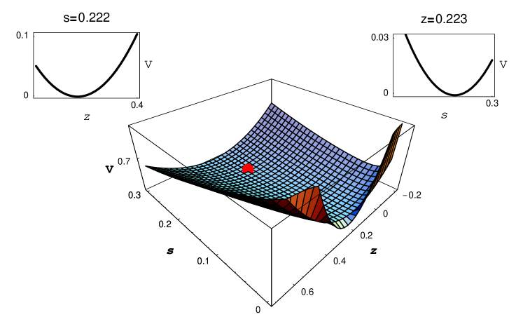
Figure 1: The picture illustrates formation of a supersymmetry breaking minimum in the supergravity scalar potential when superpotential depends on a single combination of moduli, and the shift symmetry is gauged. For better illustration somewhat unrealistic values of parameters were assumed: $\gamma=0$, $w=.1,w2=.01,{Z}_{0}=0.24,g^{2}=.001,M_{P}=50,c=\sqrt{2}$.

Using the above formulae for $F$-terms and $D$-terms one can compute the corrections to physical masses of matter scalars in the background corresponding to the minimum which we have found. The contribution due to the $F$-terms is

$$\delta_{F}m^{2}=\frac{8}{3({S}+\bar{S})^{2}}\left(\frac{Z_{0}}{M_{P}}\right)^{3}\left(\frac{w}{M_{P}^{2}}\right)^{2},$$ (23)

and the contribution due to the $D$-term looks as follows

$$\delta_{D}m^{2}=gQ\frac{w^{2}}{4{Z}_{0}^{2}M_{P}^{2}},$$ (24)

where $Q$ is the $U(1)$ charge of a scalar field. One can see that gravitational suppression of the $D$-term contribution is milder, hence for $U(1)$-charged matter this contribution shall dominate.

5 Superpotential dependent on two combinations of moduli

We have seen that the presence of moduli dependent $D$-terms associated with a gauging of some noncompact symmetry of the moduli space leads to supersymmetry breaking stable vacua in generalized racetrack models. The assumption that has been made so far is that it is a single combination of moduli fields that enters the racetrack superpotential, i.e. that coefficients $c_{i}$ in the kinetic functions for both gauge groups are the same. Fortunately, it is possible to check that a mild splitting between $c_{1}$ and $c_{2}$ doesn’t spoil validity of our observations.

Let us set

$$f_{1}=S+c_{1}M\equiv{Z}, f_{2}=S+c_{2}M\equiv S(1-c_{2}/c_{1})+{Z}c_{2}/c_{1},$$ (25)

where $c_{2}-c_{1}\equiv\eta$ and $\eta\ll 1$. The Kähler potential takes the form (3), but the superpotential obtains a correction

$$W({Z},{S})=w+({Z}-{Z}_{0})^{2}w_{2}-\eta h({Z}-{S}),$$ (26)

where $h=\frac{\beta}{c_{1}{\widetilde{b_{2}}}}e^{-\frac{{Z}}{{\widetilde{b_{2}}}}}$ is approximated by a constant. With this changes taken into account the scalar potential assumes the standard supersymmetric form, where $K$ and $W$ are given by (3) and (26), and the $D$-term is given by (11). One finds a supersymmetry breaking minimum at the point ${Z}={Z}_{0}(1+\delta_{split})$, $S={Z}$, with the complete expression for $\delta_{split}$ given by the formula (6) in the appendix. By inspection of the expressions for the $F$-terms one finds that this time it is impossible to have simultaneously $F^{S}=0$ and $F^{Z}=0$. Thus after the splitting of gauge kinetic functions there appears a supersymmetry breaking vacuum without introducing gravitational corrections. In this minimum $\langle D\rangle=0$. When one considers instead the full supergravity scalar potential, the situation becomes qualitatively very similar to the one described already in the case of two identical gauge kinetic functions. Numerical analysis of the complete model with two exponentials in the superpotential confirms above observations.

6 Summary

We have investigated moduli stabilization and supersymmetry breakdown in racetrack models with two moduli fields simultaneously present in the effective racetrack superpotential. We have demonstrated that stabilization of moduli occurs when a shift symmetry of the moduli space becomes gauged. This gauging results in a $D$-term contribution to the scalar potential that depends on moduli scalars.
To break supersymmetry at a minimum created this way in the case where only a single combination of moduli is present in the superpotential one needs to switch on supergravity corrections. Then $F$-terms of all moduli as well as the expectation value of the $D$-term are non-zero, and it is the $D$-term contribution that dominates soft scalar masses. If the superpotential depends on two independent combinations of moduli, then supersymmetry is broken by non-vanishing $F$-terms even without supergravity corrections. Some of the minima that we see correspond to a non-vanishing expectation value of the blowing-up modulus (M) in the case of type IIB orientifold models.
In addition, we have pointed out, that the gauge boson associated with gauged shift symmetry becomes higgsed and its mass may be naturally light in warped compactifications.

Acknowledgments

This work was partially supported by the EC Contract HPRN-CT-2000-00152 for years 2000-2004, by the Polish State Committee for Scientific Research grant KBN 5 P03B 119 20 for years 2001-2002, and by POLONIUM 2002.

Appendix

In the model with only a single combination of moduli present in the superpotential, and with gauged imaginary translations there appears a minimum located at the point

$$S={Z}_{0}\Big{(}1+\epsilon\Big{)},\;\;{Z}={Z}_{0}\Big{(}1+\delta\Big{)},$$ (A.1)

with

$$\epsilon=\frac{w\left(c^{2}ww_{2}\left(w+c^{2}{M_{P}}^{2}w_{2}\right)+2{M_{P}}^{3}{Z}_{0}\left(w-4w_{2}{{Z}_{0}}^{2}\right)g\right)}{2c^{2}w^{2}w_{2}\left(w+c^{2}{M_{P}}^{2}w_{2}+6w_{2}{{Z}_{0}}^{2}\right)+4{M_{P}}^{3}{Z}_{0}\left(w^{2}+2w_{2}\left(w-c^{2}{M_{P}}^{2}w_{2}\right){{Z}_{0}}^{2}-8{w_{2}}^{2}{{Z}_{0}}^{4}\right)g},$$

and $\delta$ is given by

$$\delta=\frac{3c^{2}w^{3}w_{2}+2{M_{P}}^{3}w{Z}_{0}\left(w-4w_{2}{{Z}_{0}}^{2}\right)g}{2c^{2}w^{2}w_{2}\left(w+c^{2}{M_{P}}^{2}w_{2}+6w_{2}{{Z}_{0}}^{2}\right)+4{M_{P}}^{3}{Z}_{0}\left(w^{2}+2w_{2}\left(w-c^{2}{M_{P}}^{2}w_{2}\right){{Z}_{0}}^{2}-8{w_{2}}^{2}{{Z}_{0}}^{4}\right)g}.$$

One can calculate vacuum expectation values of the $F$-terms:

$$F^{Z}= \frac{-2{\sqrt{2}}w{\left(\frac{{Z}_{0}}{{M_{P}}}\right)}^{\frac{3}{2}}}{{M_{P}}}+\frac{2{\sqrt{2}}{\left(\frac{{Z}_{0}}{{M_{P}}}\right)}^{\frac{3}{2}}\left(w+c^{2}{M_{P}}^{2}w_{2}+4w_{2}{{Z}_{0}}^{2}\right)\delta}{{M_{P}}}$$

$$+\frac{{2\sqrt{2}}\left(w-c^{2}{M_{P}}^{2}w_{2}\right){{Z}_{0}}^{3}{\sqrt{\frac{{Z}_{0}}{{M_{P}}}}}{\delta}^{2}}{c^{2}{M_{P}}^{4}}$$

$$+\left(\frac{-5{\sqrt{2}}w{\left(\frac{{Z}_{0}}{{M_{P}}}\right)}^{\frac{3}{2}}}{{M_{P}}}+\frac{{\sqrt{2}}{\left(\frac{{Z}_{0}}{{M_{P}}}\right)}^{\frac{3}{2}}\left(c^{4}{M_{P}}^{4}w_{2}-4w{{Z}_{0}}^{2}+c^{2}{M_{P}}^{2}\left(w+20w_{2}{{Z}_{0}}^{2}\right)\right)\delta}{c^{2}{M_{P}}^{3}}\right)\epsilon$$

$$+\frac{w{\left(\frac{{Z}_{0}}{{M_{P}}}\right)}^{\frac{3}{2}}\left(-7c^{2}{M_{P}}^{2}+8{{Z}_{0}}^{2}\right){\epsilon}^{2}}{2{\sqrt{2}}c^{2}{M_{P}}^{3}}+\dots+\gamma\left(\frac{-16{\sqrt{2}}w{{Z}_{0}}^{3}{\sqrt{\frac{{Z}_{0}}{{M_{P}}}}}{\delta}^{3}}{c^{2}{M_{P}}^{4}}\right.$$

$$-\frac{24{\sqrt{2}}w_{2}{{Z}_{0}}^{3}{\sqrt{\frac{{Z}_{0}}{{M_{P}}}}}{\delta}^{3}}{{M_{P}}^{2}}+\frac{48{\sqrt{2}}w{{Z}_{0}}^{3}{\sqrt{\frac{{Z}_{0}}{{M_{P}}}}}{\delta}^{2}\epsilon}{c^{2}{M_{P}}^{4}}+\frac{48{\sqrt{2}}w_{2}{{Z}_{0}}^{3}{\sqrt{\frac{{Z}_{0}}{{M_{P}}}}}{\delta}^{2}\epsilon}{{M_{P}}^{2}}$$

$$\left.-\frac{48{\sqrt{2}}w{{Z}_{0}}^{3}{\sqrt{\frac{{Z}_{0}}{{M_{P}}}}}\delta{\epsilon}^{2}}{c^{2}{M_{P}}^{4}}-\frac{24{\sqrt{2}}w_{2}{{Z}_{0}}^{3}{\sqrt{\frac{{Z}_{0}}{{M_{P}}}}}\delta{\epsilon}^{2}}{{M_{P}}^{2}}+\frac{16{\sqrt{2}}w{{Z}_{0}}^{3}{\sqrt{\frac{{Z}_{0}}{{M_{P}}}}}{\epsilon}^{3}}{c^{2}{M_{P}}^{4}}\right),$$

$$F^{S}= \frac{-2{\sqrt{2}}w{\left(\frac{{Z}_{0}}{{M_{P}}}\right)}^{\frac{3}{2}}}{{M_{P}}}+\frac{8{\sqrt{2}}w_{2}{{Z}_{0}}^{3}{\sqrt{\frac{{Z}_{0}}{{M_{P}}}}}\delta}{{M_{P}}^{2}}+\frac{{2\sqrt{2}}\left(w-c^{2}{M_{P}}^{2}w_{2}\right){{Z}_{0}}^{3}{\sqrt{\frac{{Z}_{0}}{{M_{P}}}}}{\delta}^{2}}{c^{2}{M_{P}}^{4}}$$

$$+\left(\frac{-3{\sqrt{2}}w{\left(\frac{{Z}_{0}}{{M_{P}}}\right)}^{\frac{3}{2}}}{{M_{P}}}+\frac{4{\sqrt{2}}\left(-w+5c^{2}{M_{P}}^{2}w_{2}\right){{Z}_{0}}^{3}{\sqrt{\frac{{Z}_{0}}{{M_{P}}}}}\delta}{c^{2}{M_{P}}^{4}}\right)\epsilon$$

$$+\frac{w{\left(\frac{{Z}_{0}}{{M_{P}}}\right)}^{\frac{3}{2}}\left(-3c^{2}{M_{P}}^{2}+8{{Z}_{0}}^{2}\right){\epsilon}^{2}}{2{\sqrt{2}}c^{2}{M_{P}}^{3}}+\dots+\gamma\left(\frac{4{\sqrt{2}}w{{Z}_{0}}^{5}{\sqrt{\frac{{Z}_{0}}{{M_{P}}}}}{\delta}^{4}}{c^{4}{M_{P}}^{6}}+\right.$$

$$-\frac{16{\sqrt{2}}w{{Z}_{0}}^{5}{\sqrt{\frac{{Z}_{0}}{{M_{P}}}}}{\delta}^{3}\epsilon}{c^{4}{M_{P}}^{6}}+\frac{24{\sqrt{2}}w{{Z}_{0}}^{5}{\sqrt{\frac{{Z}_{0}}{{M_{P}}}}}{\delta}^{2}{\epsilon}^{2}}{c^{4}{M_{P}}^{6}}$$

$$\left.-\frac{16{\sqrt{2}}w{{Z}_{0}}^{5}{\sqrt{\frac{{Z}_{0}}{{M_{P}}}}}\delta{\epsilon}^{3}}{c^{4}{M_{P}}^{6}}+\frac{4{\sqrt{2}}w{{Z}_{0}}^{5}{\sqrt{\frac{{Z}_{0}}{{M_{P}}}}}{\epsilon}^{4}}{c^{4}{M_{P}}^{6}}\right).$$

When the superpotential depends on two independent combinations of moduli, the minimum lies at the point ${Z}={Z}_{0}(1+\delta_{split})$ and $S={Z}$, where

$$\delta_{split}\approx\eta h\left(9{w_{2}}^{3}{{Z}_{0}}^{5}{\left(c^{3}{M_{P}}^{3}+4c{M_{P}}{{Z}_{0}}^{2}\right)}^{2}+2\,{\sqrt{3}}\left(9c^{2}{M_{P}}^{2}+4{{Z}_{0}}^{2}\right){\sqrt{{w_{2}}^{6}{{Z}_{0}}^{12}{\left(c^{3}{M_{P}}^{3}+4c{M_{P}}{{Z}_{0}}^{2}\right)}^{2}}}\right)$$

$$\left(2{w_{2}}^{2}{{Z}_{0}}^{4}\left(3c^{2}{M_{P}}^{2}-4{{Z}_{0}}^{2}\right)+2^{\frac{1}{3}}{\left(4{w_{2}}^{3}{{Z}_{0}}^{7}\left(9c^{2}{M_{P}}^{2}+4{{Z}_{0}}^{2}\right)+6{\sqrt{3}}{\sqrt{{w_{2}}^{6}{{Z}_{0}}^{12}{\left(c^{3}{M_{P}}^{3}+4c{M_{P}}{{Z}_{0}}^{2}\right)}^{2}}}\right)}^{\frac{2}{3}}\right)$$

$$\Bigg{/}\Bigg{(}{24{w_{2}}^{2}{{Z}_{0}}^{2}{\left(c^{2}{M_{P}}^{2}+4{{Z}_{0}}^{2}\right)}^{2}{\left(2{w_{2}}^{3}{{Z}_{0}}^{7}\left(9c^{2}{M_{P}}^{2}+4{{Z}_{0}}^{2}\right)+3{\sqrt{3}}{\sqrt{{w_{2}}^{6}{{Z}_{0}}^{12}{\left(c^{3}{M_{P}}^{3}+4c{M_{P}}{{Z}_{0}}^{2}\right)}^{2}}}\right)}^{\frac{4}{3}}}\Bigg{)}.$$

References

• [1] N. V. Krasnikov, Phys. Lett. B 193 (1987) 37.
• [2] L. J. Dixon, SLAC-PUB-5229, Talk given at 15th APS Div. of Particles and Fields General Mtg., Houston,TX, Jan 3-6, 1990.
• [3] J. A. Casas , Z. Lalak , C.  Munoz and G. G. Ross, Nucl. Phys.  B 347 (1990) 243.
• [4] G. Aldazabal, A. Font, L. E. Ibanez and G. Violero, Nucl. Phys. B 536 (1998) 29.
• [5] H. Itoyama and J. Leon, Phys. Rev. Lett.  56 (1986) 2352.
• [6] L. E. Ibanez and H. P. Nilles, Phys. Lett. B 169 (1986) 354.
• [7] T. Banks and M. Dine, Nucl. Phys. B 479 (1996) 173.
• [8] A. Falkowski, Z. Lalak and S. Pokorski, Nucl. Phys. B 613 (2001) 189.
• [9] L. E. Ibanez, R. Rabadan and A. M. Uranga, Nucl. Phys. B 576 (2000) 285.
• [10] Z. Lalak, S. Lavignac and H. P. Nilles, Nucl. Phys. B 576 (2000) 399.
• [11] E. Poppitz, Nucl. Phys. B 542 (1999) 31.
• [12] Z. Lalak, Talk given at SUSY01, Dubna, Russia, 11-17 Jun 2001, arXiv: hep-th/0109074.
• [13] S. A. Abel, G. Servant, Nucl. Phys. B 597 (2001) 3; Nucl. Phys. B 611 (2001) 43.
• [14] Z. Lalak and S. Thomas, Nucl. Phys. B 575 (2000) 151.
• [15] P. Horava and E. Witten, Nucl. Phys. B 475 (1996) 94.