BA-TH/02-439

UNIL-IPT 02-5

CERN-TH/2002-125

hep-ph/0206131

Assisting pre-big bang phenomenology
through short-lived axions

V. Bozza^1,2, M. Gasperini^3,4, M. Giovannini⁵ and G. Veneziano⁶

⁽¹⁾ Dipartimento di Fisica “E. R. Caianiello”, Università di Salerno,
Via S. Allende, 84081 Baronissi (SA), Italy
⁽²⁾ INFN, Sezione di Napoli, Gruppo Collegato di Salerno, Salerno, Italy

⁽³⁾ Dipartimento di Fisica, Università di Bari,
Via G. Amendola 173, 70126 Bari, Italy
⁽⁴⁾ INFN, Sezione di Bari, Bari, Italy

⁽⁵⁾ Institute of Theoretical Physics, University of Lausanne,
BSP-1015 Dorigny, Switzerland

⁽⁶⁾ Theoretical Physics Division, CERN, CH-1211 Geneva 23, Switzerland

We present the results of a detailed study of how isocurvature axion fluctuations are converted into adiabatic metric perturbations through axion decay, and discuss the constraints on the parameters of pre-big bang cosmology needed for consistency with present CMB-anisotropy data. The large-scale normalization of temperature fluctuations has a non-trivial dependence both on the mass and on the initial value of the axion. In the simplest, minimal models of pre-big bang inflation, consistency with the COBE normalization requires a slightly tilted (blue) spectrum, while a strictly scale-invariant spectrum requires mild modifications of the minimal backgrounds at large curvature and/or string coupling.

It is well known that, in the framework of pre-big bang cosmology (see [1, 2] for recent reviews), the primordial spectrum of scalar (and tensor) metric perturbations is characterized by a steep positive slope [3]. Since the high-frequency normalization of the spectrum is fixed by the ratio of the string to the Planck mass, the amplitude of metric fluctuations turns out to be strongly suppressed at large scales, and thus unable to account for the CMB anisotropies observed by COBE [4] and by other satellite experiments [5] (unless one accepts rather drastic modifications of pre-big bang kinematics, as recently suggested in [6]).

A possible solution to this problem could be provided, a priori, by the fluctuations of another background field of string theory, in particular of the so-called Kalb–Ramond axion $\sigma$ (the dual of the NS-NS two-form appearing in the dimensionally reduced string effective action [7]). As first pointed out in [8], axionic quantum fluctuations of the vacuum are amplified by pre-big bang inflation, yielding a final spectrum whose index $n_{\sigma}$ can vary, depending on the evolution of extra dimensions. The scale-invariant value of $n_{\sigma}=1$ is attained, amusingly enough, for particularly symmetric evolutions of the nine spatial dimensions in which critical superstrings consistently propagate.

Indeed, even if no axion potential is present in the post-big bang era, a (generally non-Gaussian) spectrum of temperature anisotropies can be induced by the fluctuations of the massless [9, 10] axion field, at second order, through the so-called “seed” mechanism [11]. The same is true for a massive light axion that has not decayed yet [12]. Unfortunately, while the model is capable of reproducing the low-multipole COBE data [4], it clearly appears [13] to be disfavoured with respect to standard inflationary models when it comes to fitting data in the acoustic-peaks region [5].

An interesting alternative possibility, first suggested in [1], and recently discussed in detail (and not exclusively within a string cosmology framework) in [14]-[18], uses a general mechanism originally pointed out in [19]. It is based on two basic assumptions: i) the constant value of the axion background after the pre-big bang phase is displaced from the minimum (conventionally defined as $\sigma=0$) of the non-perturbative potential $V(\sigma)$ generated in the post-big bang epoch; ii) the axion potential is strong enough to induce a phase of axion dominance before its decay into radiation. Under these two (rather plausible) assumptions, the initially amplified isocurvature axion fluctuations can be converted, without appreciable change of the spectrum, into adiabatic (and Gaussian) scalar curvature perturbations until the time of horizon re-entry: these can then possibly produce the observed CMB anisotropies.

Various aspects of this new mechanism have already been discussed in [14] for the string theory axion, and in [15]-[17] (mostly in the context of conventional inflationary models) for the case of a generic scalar field, dubbed the “curvaton” in [15] (see also [18] for a possible application of this mechanism to the ekpyrotic scenario). Here, after providing an explicit derivation and computation of the conversion of axion fluctuations into scalar curvature perturbations, we shall discuss the constraints imposed by the CMB data, and its possible consistency with the small-scale normalization and tilts typical of pre-big bang models. It will be argued, in particular, that a strictly flat spectrum is only compatible with non-minimal models of pre-big bang inflation. A detailed account of this work, including numerical checks of the analytic arguments and estimates given here, will be presented in a forthcoming paper [20].

The conversion of the axionic isocurvature modes (amplified during the pre-big-bang phase) into adiabatic curvature inhomogeneities takes place in the post-big-bang phase, where we assume the dilaton to be frozen and the axion to be displaced from the minimum of its potential. The relaxation of the axionic field towards the minimum of its potential is determined by the following evolution equations (units where $16\pi G=1$ are used)

$$R_{\mu}^{\nu}-{1\over 2}\delta_{\mu}^{\nu}R={1\over 2}T_{\mu}^{\nu}+{1\over 2}\partial_{\mu}\sigma\partial^{\nu}\sigma+{1\over 2}\delta_{\mu}^{\nu}\left[V-{1\over 2}(\nabla_{\mu}\sigma)^{2}\right],$$

$$\nabla_{\mu}\nabla^{\mu}\sigma+{\partial V\over\partial\sigma}=0,$$ (1)

where $T_{\mu\nu}$ is the stress tensor of the matter sources, which we assume to be dominated by the radiation fluid. In the case of a conformally flat metric, $g_{\mu\nu}=a^{2}\eta_{\mu\nu}$, the time and space components of such equations, together with the axion evolution equation, can be written (in conformal time and in three spatial dimensions) respectively as

$$6{\cal H}^{2}=a^{2}\left(\rho_{r}+\rho_{\sigma}\right),~{}~{}~{}~{}~{}~{}~{}~{}~{}~{}~{}~{}4{\cal H}^{\prime}+2{\cal H}^{2}=-a^{2}\left(p_{r}+p_{\sigma}\right),$$ (2)

$$\sigma^{\prime\prime}+2{\cal H}\sigma^{\prime}+a^{2}{\partial V\over\partial\sigma}=0,$$ (3)

where ${\cal H}=a^{\prime}/a=d(\ln a)/d\eta$, $\rho_{r}=3p_{r}$ is the energy density of the radiation fluid, and

$$\rho_{\sigma}={1\over 2a^{2}}\sigma^{\prime 2}+V(\sigma),~{}~{}~{}~{}~{}~{}~{}p_{\sigma}={1\over 2a^{2}}\sigma^{\prime 2}-V(\sigma).$$ (4)

The combination of Eqs. (2) and (3) leads to the conservation equation for the radiation fluid, i.e. $\rho_{r}^{\prime}+4{\cal H}\rho_{r}=0$.

While the background is radiation-dominated, at least at the onset of the post-big-bang phase, the initial large-scale inhomogeneities are dominated by the (isocurvature) perturbations coming from the pre-big bang amplification of the quantum fluctuations of the axion. In order to study the conversion of isocurvature into scalar curvature (adiabatic) modes, the background Eqs. (2) and (3) should be supplemented by the evolution equations of the scalar inhomogeneities, following from the perturbation of the Einstein equations (1).

Thanks to the absence of anisotropic stresses, the $i\not=j$ components of the perturbed Einstein equations imply that the scalar metric fluctuations can be parametrized in terms of a single gauge-invariant variable, the Bardeen potential $\Phi$ [21]. The full system of perturbed Einstein equations can then be written as

$$\Phi^{\prime}+{\cal H}\Phi={1\over 4}\chi\sigma^{\prime}+{1\over 3}a^{2}\rho_{r}v_{r},$$ (5)

$$\nabla^{2}\Phi-3{\cal H}\left(\Phi^{\prime}+{\cal H}\Phi\right)={1\over 4}a^{2}\left(\rho_{r}\delta_{r}+\rho_{\sigma}\delta_{\sigma}\right),$$ (6)

$$\Phi^{\prime\prime}+3{\cal H}\Phi^{\prime}+\left({2\cal H}^{\prime}+{\cal H}^{2}\right)\Phi={1\over 4}a^{2}\left({1\over 3}\rho_{r}\delta_{r}+\delta p_{\sigma}\right),$$ (7)

$$\chi^{\prime\prime}+2{\cal H}\chi^{\prime}-\nabla^{2}\chi+a^{2}{\partial^{2}V\over\partial\sigma^{2}}\chi=4\sigma^{\prime}\Phi^{\prime}-2a^{2}{\partial V\over\partial\sigma}\Phi,$$ (8)

where the gauge-invariant variables $\chi$, $\delta\rho_{r}$, $v_{r}$ are, respectively, the axion, radiation density and velocity potential fluctuations [with our conventions, in the longitudinal gauge the velocity potential is defined by $\delta T_{i}^{0}=(\rho_{r}+p_{r})\partial_{i}v_{r}$], and where the following variables

$$\delta_{r}=\delta\rho_{r}/\rho_{r},~{}~{}~{}~{}~{}~{}~{}~{}~{}~{}~{}\delta_{\sigma}=\delta\rho_{\sigma}/\rho_{\sigma},$$

$$\delta\rho_{\sigma}=-\Phi\left(\rho_{\sigma}+p_{\sigma}\right)+{\sigma^{\prime}\chi^{\prime}\over a^{2}}+{\partial V\over\partial\sigma}\chi,$$

$$\delta p_{\sigma}=-\Phi\left(\rho_{\sigma}+p_{\sigma}\right)+{\sigma^{\prime}\chi^{\prime}\over a^{2}}-{\partial V\over\partial\sigma}\chi$$ (9)

have been defined (we have also assumed $\delta p_{r}=\delta\rho_{r}/3$). By using the above perturbation equations, together with the background relations (2) and (3), two useful equations for the evolution of the radiation density contrast and of the velocity potential can be finally obtained:

$$\delta_{r}^{\prime}=4\Phi^{\prime}+{4\over 3}\nabla^{2}v_{r},~{}~{}~{}~{}~{}~{}~{}~{}~{}~{}~{}~{}v_{r}^{\prime}={1\over 4}\delta_{r}+\Phi.$$ (10)

We now suppose to start at $t=t_{i}$ with a radiation-dominated phase in which the homogeneous axion background is initially constant and non-vanishing, $\sigma(t_{i})=\sigma_{i}\not=0$, $\sigma^{\prime}(t_{i})=0$, providing a subdominant (potential) energy density, $\rho_{\sigma}(t_{i})=-p_{\sigma}(t_{i})=V_{i}$ $\ll H_{i}^{2}\sim\rho_{r}(t_{i})$. The initial conditions of Eqs. (5)–(8) are imposed by assuming a given spectrum of isocurvature axion fluctuations, $\chi_{k}(t_{i})\not=0$, and a total absence of perturbations for the metric and the radiation fluid, $\Phi(t_{i})=\delta_{r}(t_{i})=v_{r}(t_{i})=0$. The initial values of the first derivatives of the perturbation variables are then fixed by enforcing the momentum and Hamiltonian constraints, i.e. Eqs. (5) and (6).

Before discussing the origin of curvature fluctuations we must specify the details of the background evolution. The axion, initially constant and subdominant, starts oscillating at a curvature scale $H_{\rm osc}\sim m$ (as can be argued from Eq. (3)), and eventually decays (with gravitational strength) into radiation, at a scale $H_{d}\sim m^{3}/M_{\rm P}^{2}<H_{\rm osc}$ (a process that must occur early enough, not to disturb the subsequent standard evolution). When the axion is constant, $\rho_{\sigma}$ behaves like an effective cosmological constant, while during the oscillatory phase its kinetic and potential energy density are equal on the average, so that $\langle p_{\sigma}\rangle=0$, and $\langle\rho_{\sigma}\rangle\sim a^{-3}$ behaves like dust matter. Thus the radiation energy is always diluted faster, $\rho_{r}\sim a^{-4}$, and the axion background tends to become dominant at a scale $H_{\sigma}(t)\sim\sqrt{V[\sigma(t)]}$.

For an efficient conversion of the initial $\chi$ and $\delta_{\sigma}$ fluctuations into $\Phi$ and $\delta_{r}$ fluctuations it is further required [14]-[16], as we shall see, that the decay occur after the beginning of the axion-dominated phase, i.e. when $H_{\sigma}>H_{d}$. Depending upon the relative values of $H_{\sigma}$ and $H_{\rm osc}$ (i.e. depending upon the value of $\sigma_{i}$ in Planck units) we have two different options which will now be discussed separately. In order to perform explicit analytical estimates, we shall assume here that $V(\sigma)$ can be approximated by the quadratic form $m^{2}\sigma^{2}/2$. This is certainly true for $\sigma_{i}\ll 1$, but it may be expected to be a realistic approximation also for the range of values of $\sigma_{i}$ not much larger than $1$ (which, as we shall see, is the appropriate range for a normalization of the spectrum compatible with present data). Actually, for the periodic potential expected for an axion the value of $|\sigma_{i}|$ is effectively bounded from above [14].

$(1)$ If $\sigma_{i}<1$ then $H_{\sigma}<H_{\rm osc}$, and the axion starts oscillating (at a scale $H\sim m$) when the Universe is still radiation-dominated. During the oscillations the average potential energy density decreases like $a^{-3}$, i.e. the typical amplitude of oscillation decreases, following an $a^{-3/2}$ law, from its initial value $\sigma_{i}$ to the value $\sigma_{\rm dom}$ at which $H=H_{\sigma}\sim m\sigma_{\rm dom}$. During this period $a\sim H^{-1/2}$ (as the background is radiation-dominated), so that $\sigma_{\rm dom}\sim\sigma_{i}^{4}$, and $H_{\sigma}\sim m\sigma_{i}^{4}$. Finally, the background remains axion-dominated until the decay scale $H_{d}\sim m^{3}/M_{\rm P}^{2}$. This model of background is thus consistent for $H_{i}>H_{\rm osc}>H_{\sigma}>H_{d}$, namely for

$$1>\sigma_{i}>(m/M_{\rm P})^{1/2},$$ (11)

which allows for a wide range for $\sigma_{i}$, if we recall the cosmological bounds on the mass following from the decay of a gravitationally coupled scalar [22] (typically, $m>10$ TeV to avoid disturbing standard nucleosynthesis).

$(2)$ If $\sigma_{i}>1$, and then $H_{\sigma}>H_{\rm osc}$, the axion starts dominating at the scale $H_{\sigma}\sim m\sigma_{i}$, which marks the beginning of a phase of slow-roll inflation, lasting until the curvature drops below the oscillation scale $H_{\rm osc}\sim m$. Such a model of background is consistent for $H_{\sigma}<H_{1}$, namely for

$${H_{1}/m}>\sigma_{i}>1,$$ (12)

where $H_{1}$ (fixed around the string scale) corresponds to the beginning of the radiation-dominated, post-big bang evolution. During the inflationary phase the slow decrease of the Hubble scale can be approximated (according to the background equations (2) and (3)) by $H(t)=\alpha m\sigma_{i}-\beta m^{2}(t-t_{\sigma})$, where $\alpha$ and $\beta$ are dimensionless coefficients of order $1$. Inflation thus begins at the epoch $t=t_{\sigma}\sim 1/m\sigma_{i}$, and lasts until the epoch $t=t_{m}\sim(\sigma_{i}-1)/m\sim\sigma_{i}/m$.

Finally, if $\sigma_{i}\sim 1$, $H_{\sigma}\sim H_{\rm osc}\sim m$, and the beginning of the oscillating and of the axion-dominated phase are nearly simultaneous. Let us now estimate, for these classes of backgrounds, the evolution of the Bardeen potential generated by the primordial axion fluctuations.

It is convenient, for this purpose, to introduce the gauge-invariant variable $\zeta$ representing the spatial curvature perturbation on uniform density (or equivalently, at large scales, on comoving) hypersurfaces. For purely adiabatic perturbations $\zeta$ is conserved (outside the horizon), and can be written for a general background as [21]:

$$\zeta=-\Phi-{{\cal H}\Phi^{\prime}+{\cal H}^{2}\Phi\over{\cal H}^{2}-{\cal H}^{\prime}}.$$ (13)

Outside the horizon, Eq. (10) gives $4\Phi=\delta_{r}$; the sum of the two background equations (2) for the denominator ${\cal H}^{2}-{\cal H}^{\prime}$ and the Hamiltonian constraint (6) for the numerator ${\cal H}\Phi^{\prime}+{\cal H}^{2}\Phi$, allow $\zeta$ to be rewritten in the convenient form

$$\zeta_{k}={\rho_{\sigma}\delta_{\sigma}(k)-(3/4)(\rho_{\sigma}+p_{\sigma})\delta_{r}(k)\over 4\rho_{r}+3(\rho_{\sigma}+p_{\sigma})}.$$ (14)

This expression has been obtained by neglecting the contribution of spatial gradients in Eqs. (5)–(8). Numerical integration shows [20] that the corrections coming from these terms are indeed negligible for the large-scale modes leading to the anisotropies in the CMB.

Consider now the beginning of the post-big bang phase, when the radiation dominates the background while the axion dominates the fluctuations. In this case Eq. (14) gives immediately:

$$\zeta_{k}={1\over 4}~{}{\rho_{\sigma}\delta_{\sigma}(k)\over\rho_{r}}=\frac{1}{4\rho_{r}}\frac{\partial V}{\partial\sigma}\chi_{k}=\frac{1}{24}\frac{a^{2}}{{\cal H}^{2}}\frac{\partial V}{\partial\sigma}\chi_{k}\propto a^{4},$$ (15)

where we have used the fact that, in the initial phase, $\sigma$ is approximately constant. Since also $\Phi_{k}$ will behave like $a^{4}$, it is easy to find its relation to $\zeta$ using, inside (13), $\Phi^{\prime}=4{\cal H}\Phi$ and ${\cal H}^{\prime}=-{\cal H}^{2}$, with the result:

$$\Phi_{k}=-\frac{2}{7}\zeta_{k}=-\frac{1}{14}~{}{\rho_{\sigma}\delta_{\sigma}(k)\over\rho_{r}}.$$ (16)

In order to proceed further, two alternatives (already discussed in the context of the background evolution) should now be separately examined:

$(1)$ If $\sigma_{i}<1$, during the oscillating (but still radiation-dominated) phase, $\zeta$ can still be obtained from Eq. (14), but now $\rho_{\sigma}\sim\delta\rho_{\sigma}\sim a^{-3}$, and $\zeta$ will evolve like $a\sim\eta\sim t^{1/2}$. Since $a$ changes by a factor $(m/H_{\sigma})^{1/2}\simeq(\sigma_{i})^{-2}$, we end up with a value of $\zeta_{k}$ at $t_{\sigma}$ given by:

$$\zeta_{k}(t_{\sigma})\sim{\chi_{k}(t_{i})\over\sigma_{i}},~{}~{}~{}~{}~{}~{}~{}~{}~{}~{}~{}~{}~{}~{}~{}~{}\sigma_{i}\leq 1.$$ (17)

On the other hand, using again Eq. (13) and the appropriate relations in the oscillating, radiation-dominated phase, we find $\Phi_{k}(t_{\sigma})=-\zeta_{k}(t_{\sigma})/2$. In the final phase, dominated by an oscillating axion, $\rho_{r}$ is negligible, the (average) axion pressure is zero, and (the average of) $\Phi_{k}$ is constant, as well as the average of $\zeta_{k}$, which oscillates around a final amplitude of the same order as $\zeta_{k}(t_{\sigma})$ given in eq. (17). This implies, through Eqs. (5), (6) and (10), $\delta_{\sigma}(k)=-2\Phi_{k}=-(1/2)\delta_{r}(k)$, so that, from Eq. (13) we are led to

$$\langle\zeta_{k}\rangle=-{5\over 3}\langle\Phi_{k}\rangle={5\over 6}\langle\delta_{\sigma}(k)\rangle,$$ (18)

where $\langle...\rangle$ refers to averages over one oscillation period. We have checked the validity of this result by an explicit numerical integration (the same result has already been presented in [15], using different notations).

$(2)$ If $\sigma_{i}>1$, then Eq. (14) can still be used until $t_{\sigma}=1/m\sigma_{i}$, where we find:

$$\zeta_{k}(t_{\sigma})=\frac{1}{4\rho_{\sigma}}~{}\frac{\partial V}{\partial\sigma}\chi_{k}\sim{\chi_{k}(t_{i})\over\sigma_{i}}.$$ (19)

During the period of axion-dominated slow-roll inflation, Eq. (14) is still valid. However, since $\rho_{r}$ soon becomes subdominant with respect to $\rho_{\sigma}+p_{\sigma}$, it should be appreciated that at the end of the slow-roll period the latter term is of order $m^{2}$, and the resulting estimate will thus be:

$$\zeta_{k}(t_{m})={1\over 4}~{}\frac{\partial V}{\partial\sigma}{\chi_{k}\over m^{2}}\sim{\chi_{k}(t_{i})\sigma_{i}},~{}~{}~{}~{}~{}~{}~{}~{}~{}~{}~{}~{}~{}~{}~{}\sigma_{i}>1.$$ (20)

Note that this formula is in (qualitative) agreement with Eq. (18), if we use $\delta\rho_{\sigma}\sim m^{2}\chi_{k}(t_{i})\sigma_{i}$ and $\rho_{\sigma}\sim m^{2}$. No further amplification is expected in the course of the subsequent cosmological evolution. Similar expressions hold for the amplitude of $\Phi_{k}$, related to $\zeta_{k}$ by Eq. (18).

It is amusing to observe that the results (17), (20), which determine the amplitude of the Bardeen potential in the oscillating (axion-dominated) phase preceding the moment ($t=t_{d}$) at which the decay occurs, can be summarized by an equation that holds in all cases, namely

$$\langle\Phi_{k}(t_{d})\rangle=-\chi_{k}(t_{i})f(\sigma_{i}),~{}~{}~{}~{}~{}~{}~{}~{}~{}~{}~{}f(\sigma_{i})=\left(c_{1}\sigma_{i}+{c_{2}\over\sigma_{i}}+c_{3}\right),$$ (21)

where $c_{1},c_{2},c_{3}$ are numerical coefficients of the order of unity. A preliminary fit based on numerical and analytical integrations of the perturbation equations gives $c_{1}=0.129,c_{2}=0.183,c_{3}=0.019$ (see [20] for further details). The function $f(\sigma_{i})$ has the interesting feature that it is approximately invariant under the transformation $\sigma_{i}\rightarrow\sigma_{i}^{-1}$ and, as a consequence, has a minimal value around $\sigma_{i}=1$, a result we shall use later on.

The generated spectrum of super-horizon curvature perturbations is thus directly determined by the primordial spectrum of isocurvature axion fluctuations $\chi_{k}$, according to Eqs. (17) and (20). The axion fluctuations, on the other hand, are solutions (with pre-big bang initial conditions) of Eq. (8) in the radiation era (no additional amplification is expected, for super-horizon modes, in the axion-dominated phase), computed for negligible curvature perturbations ($\Phi=0=\Phi^{\prime}$), evaluated in the massive, non-relativistic limit (where we are, eventually, in the oscillating regime) and outside the horizon. The exact solution for $\chi_{k}$, normalized to a relativistic spectrum of quantum fluctuations (amplified with the Bogoliubov coefficient $c_{k}$) has already been computed in [10]. Setting $x=\eta\sqrt{2\alpha}$, $\alpha=mH_{1}a_{1}^{2}$, $b=-k^{2}/2\alpha$, it can be written in the form

$$\chi_{k}={c_{k}\over a}\left(k\over 2\alpha\right)^{1/2}y_{2}(b,x),$$ (22)

where $y_{2}$ is the odd part of the parabolic cylinder functions [23]. Outside the horizon ($-bx^{2}\ll 1$) and for non-relativistic modes ($-b\ll x^{2}$), the solution can be expanded, to leading order, as $y_{2}\sim x=\eta\sqrt{2\alpha}$. By inserting a generic power-law spectrum, with cut-off scale $k_{1}=H_{1}a_{1}$ and spectral index $n$, i.e. $|c_{k}|=(k/k_{1})^{(n-5)/2}$, we finally obtain the generated spectrum of curvature perturbations:

$$k^{3}\left|\Phi_{k}\right|^{2}=f^{2}(\sigma_{i}){k^{3}}\left|\chi_{k}\right|^{2}=f^{2}(\sigma_{i})\left(H_{1}\over M_{\rm P}\right)^{2}\left(k\over k_{1}\right)^{n-1},~{}~{}~{}~{}~{}~{}~{}~{}~{}~{}~{}~{}~{}~{}~{}k<k_{1}$$ (23)

(we have absorbed into the definition of $k_{1}$ possible numerical factors of order one connecting the cut-off scale to the string mass).

Note that we have re-inserted the appropriate Planck mass factors, keeping $\sigma_{i}$ dimensionless. It may be useful to recall that the spectral index $n$ depends upon the pre big-bang dynamics [8], and that for an isotropic $6$-dimensional subspace it can be written in the form [13]

$$n=\frac{4+6r^{2}-2\sqrt{3+6r^{2}}}{1+3r^{2}},$$ (24)

where $r=(\dot{V}_{6}V_{3})/(2V_{6}\dot{V}_{3})$ accounts for the relative rate of variation of the six-dimensional internal volume $V_{6}$ and of the “external” (usual) volume $V_{3}$. As already mentioned, the case of a flat spectrum (i.e. $n=1$) corresponds to $r=\pm 1$. Otherwise, $n$ increases monotonically with $r^{2}$ from the value $n=4-2\sqrt{3}\simeq 0.53$ when internal dimensions are static ($r=0$), to $n=2$ for the case of a static external manifold ($r\to\infty$).

The result (23) is valid during the axion-dominated phase, and has to be transferred to the phase of standard evolution, by matching the (well-known [21]) solution for the Bardeen potential in the radiation era (subsequent to axion decay) to the solution prior to decay, which is in general oscillating. The matching of $\Phi$ and $\Phi^{\prime}$, conventionally performed at the fixed scale $H=H_{d}$, shows that the constant asymptotic value (21) of super-horizon modes is preserved (to leading order) by the decay process, modulo a random, mass-dependent correction which typically takes the form $1+\epsilon\sin(m/H_{d})$, with $\epsilon$ a numerical coefficient of order $1$, and $m/H_{d}\gg 1$. Such a random factor, however, is a consequence of the sudden approximation adopted to describe the decay process, and disappears in a more realistic treatment in which the axion equation (3) is supplemented by the friction term $+\Gamma{\sigma^{\prime}}/{a}$ (leading to the term $+\Gamma{{\sigma^{\prime}}^{2}}/{a^{2}}$ in the equation for $\rho_{\sigma}$), and a corresponding antifriction term $-\Gamma{{\sigma^{\prime}}^{2}}/{a^{2}}$ in the radiation equation. The axion fluctuations will follow the background and decay with a similar term, $+\Gamma{\chi^{\prime}}/{a}$, in the perturbation equation (8).

The previous analysis performed up to $t=t_{d}$ remains valid for the modified equations, since for $\Gamma\ll H$ the decay terms are negligible. We have checked with a numerical integration [20] that the decay process preserves the value of the Bardeen potential prior to decay, damping the residual oscillations; $\zeta$ itself follows the same behaviour and is finally exactly a constant. When the axion has completely decayed, and the Universe is again dominated by radiation, we can properly match the standard evolution of $\Phi$ in the radiation phase to the constant asymptotic value of Eq. (21). The expression we obtain for the (oscillating) Bardeen potential, valid until the epoch of matter–radiation equality (denoted in the following by $\eta_{\rm eq}$), can be written in the form

$$\Phi_{k}(\eta)=-3\Phi_{k}(\eta_{d})\biggl{[}\frac{\cos{(kc_{s}\eta)}}{(kc_{s}\eta)^{2}}-\frac{\sin{(kc_{s}\eta)}}{(kc_{s}\eta)^{3}}\biggr{]},~{}~{}~{}~{}~{}~{}~{}~{}~{}\eta_{d}<\eta<\eta_{\rm eq},$$ (25)

where $c_{s}=1/\sqrt{3}$ and $\Phi_{k}(\eta_{d})$ is given in Eq. (21).

The above expression for the Bardeen potential provides the initial condition for the evolution of the CMB-temperature fluctuations, and the formation of their oscillatory pattern. Standard results [24] (see also [25]) imply that the patterns of the CMB anisotropies (and, in particular, the position of the first Doppler peak) are related to the sum of two oscillating contributions, with a relative phase of $\pi/2$. Denoting by $\eta_{\rm dec}$ the decoupling time, the first contribution oscillates like $A\cos{[kr_{s}(\eta_{\rm dec})]}$, while the second one oscillates like $B\sin{[kr_{s}(\eta_{\rm dec})]}$, where $r_{s}(\eta_{\rm dec})$ is the sound-horizon at $\eta=\eta_{\rm dec}$. The value of $\Phi_{k}$ for $\eta\ll\eta_{\rm eq}<\eta_{\rm dec}$ determines, in particular, the relative phase of oscillation of the two terms. In our case, from Eq. (25), $\Phi_{k}(\eta_{i})={\rm constant}$ and $\Phi^{\prime}_{k}(\eta_{i})\simeq 0$, where $\eta_{d}<\eta_{i}<\eta_{\rm eq}$, and $k\eta_{i}\ll 1$. This implies $B=0$, so that the temperature anisotropies $(\Delta T/T)_{k}$ will oscillate like [24] $\Phi_{k}(\eta_{i})\cos{[kr_{s}(\eta_{\rm dec})]}$, as is generally the case for adiabatic fluctuations. The opposite case, $\Phi_{k}(\eta_{i})\simeq 0$ and $\Phi_{k}^{\prime}(\eta_{i})=$ constant, corresponds instead to isocurvature initial conditions [26], producing a peak structure that is clearly distinguishable from the adiabatic case and, at present, observationally disfavoured.

After checking that the above scenario leads to the standard adiabatic mode, producing the observed peak structure of the CMB anisotropies, we still have to discuss the possibility of a correct large-scale normalization of the spectrum, compatible with the COBE data. We start from the observation that the final amplitude of the super-horizon perturbations (23), just like the spectral slope, is not at all affected by the non-relativistic corrections to the axion spectrum [12], in spite of the crucial role played by the mass in the decay process (see also [14]). The mass dependence reappears, however, when computing the amplitude of the spectrum at the present horizon scale $\omega_{0}$, in order to impose the corrected normalization to the quadrupole coefficient $C_{2}$ determined by COBE, namely [27]

$$C_{2}=\alpha^{2}_{n}f^{2}(\sigma_{i})\left(H_{1}\over M_{\rm P}\right)^{2}\left(\omega_{0}\over\omega_{1}\right)^{n-1},~{}~{}~{}~{}~{}~{}~{}\alpha_{n}^{2}={2^{n}\over 72}{\Gamma(3-n)\Gamma\left({3+n\over 2}\right)\over\Gamma^{2}\left({4-n\over 2}\right)\Gamma\left({9-n\over 2}\right)},$$ (26)

where [28] $C_{2}=(1.9\pm 0.23)\times 10^{-10}$.

The present value of the cut-off frequency, $\omega_{1}(t_{0})=H_{1}a_{1}/a_{0}$, depends in fact on the kinematics as well as on the duration of the axion-dominated phase (and thus on the axion mass), as follows:

$$\omega_{1}(t_{0}) = H_{1}\left(a_{1}\over a_{\sigma}\right)_{\rm rad}\left(a_{\sigma}\over a_{d}\right)_{\rm mat}\left(a_{d}\over a_{\rm eq}\right)_{\rm rad}\left(a_{\rm eq}\over a_{0}\right)_{\rm mat},~{}~{}~{}~{}~{}~{}~{}~{}~{}~{}~{}~{}~{}~{}~{}~{}~{}\sigma_{i}<1,$$ (27)

$$= H_{1}\left(a_{1}\over a_{\sigma}\right)_{\rm rad}\left(a_{\sigma}\over a_{\rm osc}\right)_{\rm inf}\left(a_{\rm osc}\over a_{d}\right)_{\rm mat}\left(a_{d}\over a_{\rm eq}\right)_{\rm rad}\left(a_{\rm eq}\over a_{0}\right)_{\rm mat},~{}~{}~{}\sigma_{i}>1.$$ (28)

Using $H_{0}\simeq 10^{-6}H_{\rm eq}\simeq 10^{-61}M_{\rm P}$ we find

$${\omega_{0}\over\omega_{1}} \simeq 10^{-29}\left(H_{1}\over M_{\rm P}\right)^{-1/2}\left(m\over\sigma_{i}^{2}M_{\rm P}\right)^{-1/3},~{}~{}~{}~{}~{}~{}~{}~{}~{}~{}~{}~{}~{}~{}~{}~{}~{}\sigma_{i}<1,$$ (29)

$$\simeq 10^{-29}\left(\sigma_{i}H_{1}\over M_{\rm P}\right)^{-1/2}\left(m\over\ M_{\rm P}\right)^{-1/3}Z_{\sigma},~{}~{}~{}~{}~{}~{}~{}~{}~{}~{}~{}~{}~{}~{}\sigma_{i}>1,$$ (30)

where $Z_{\sigma}=(a_{\rm osc}/a_{\sigma})$ denotes the amplification of the scale factor during the phase of axion-dominated, slow-roll inflation. The COBE normalization thus imposes

$$c_{2}^{2}\alpha^{2}_{n}\sigma_{i}^{2(n-4)/3}\left(H_{1}\over M_{\rm P}\right)^{(5-n)/2}\left(m\over M_{\rm P}\right)^{-(n-1)/3}10^{-29(n-1)}\simeq 10^{-10},~{}~{}~{}~{}~{}~{}~{}~{}\sigma_{i}<1,$$ (31)

$$c_{1}^{2}\alpha^{2}_{n}Z_{\sigma}^{n-1}\sigma_{i}^{(5-n)/2}\left(H_{1}\over M_{\rm P}\right)^{(5-n)/2}\left(m\over M_{\rm P}\right)^{-(n-1)/3}10^{-29(n-1)}\simeq 10^{-10},~{}~{}~{}\sigma_{i}>1.$$ (32)

We can notice, as a side remark, that the contribution of the gradients appearing in Eqs. (5)–(8) follows the same hierarchy of scales as provided by Eqs. (29), (30) and this is the reason why, ultimately, the contribution of the gradients can be neglected as far as the evolution of large-scale modes is concerned.

The condition (31) is to be combined with the constraint (11), the condition (32) with the constraint (12), which are required for the consistency of the corresponding classes of background evolution. Also, both conditions are to be intersected with the experimentally allowed range of the spectral index. Finally, in the case $\sigma_{i}>1$ we are also implicitly assuming that the axion-driven inflation is short enough to avoid a possible contribution to $C_{2}$ arising from the metric fluctuations directly amplified from the vacuum, during the phase of axionic inflation. This requires that the smallest amplified frequency mode $\omega_{\sigma}$, crossing the horizon at the beginning of inflation, be today still larger than the present horizon scale $\omega_{0}$. This imposes the condition $\omega_{\sigma}(t_{0})=H_{\sigma}(a_{\sigma}/a_{0})>\omega_{0}$, namely

$$Z_{\sigma}~{}\raise 1.72218pt\hbox{$<$}\kern-8.00003pt\lower 2.6694pt\hbox{$\sim$}~{}10^{29}\sigma_{i}\left(m\over M_{\rm P}\right)^{5/6},$$ (33)

to be added to the constraint (12) for $\sigma_{i}>1$. It turns out, however, that this condition is always automatically satisfied for the range of spectral indices we are interested in (in particular, for $n\leq 1.7$).

The allowed range of parameters compatible with all constraints is rather strongly sensitive to the values of the pre-big bang inflation scale $H_{1}$. In the context of minimal models of pre-big bang inflation [3] we have $H_{1}\sim M_{s}$, and a flat spectrum ($n=1$) is inconsistent with the normalization (31), (32). A growing (“blue”) spectrum is instead allowed, and by setting for instance $c_{2}\alpha_{n}H_{1}/M_{\rm P}=10^{-2}$, using (as a reference value) the upper bound [29] $n<1.4$, and considering the case $\sigma_{i}\leq 1$, we find a wide range of allowed axion masses, but a rather narrow range of allowed values for $\sigma_{i}$, namely $1~{}\raise 1.72218pt\hbox{$>$}\kern-6.99997pt\lower 2.6694pt\hbox{$\sim$}~{}\sigma_{i}~{}\raise 1.72218pt\hbox{$>$}\kern-6.99997pt\lower 2.6694pt\hbox{$\sim$}~{}10^{-5/2}$, and of allowed values for the spectral index, $n\simeq 1.22$–$1.4$. In the case $\sigma_{i}>1$ the results are complementary for the spectral index, but there are much more stringent bounds for $\sigma_{i}$, because the inflationary redshift factor $Z_{\sigma}$ grows exponentially with $\sigma_{i}^{2}$, in such a way that the COBE normalization (32) cannot be satisfied, unless the upper value of $\sigma_{i}$ is strongly bounded. This means that the apparent symmetry between the $\sigma_{i}<1$ and the $\sigma_{i}>1$ cases is broken by the requirement of the CMB normalization, which forbids too large values of $\sigma_{i}$.

The allowed region may be further extended if the inflation scale $H_{1}$ is lowered, and a flat ($n=1$) spectrum may become possible if $c_{2}\alpha_{n}H_{1}~{}\raise 1.72218pt\hbox{$<$}\kern-8.00003pt\lower 2.6694pt\hbox{$\sim$}~{}10^{-5}M_{\rm P}\sigma_{i}$, for $\sigma_{i}<1$, and if $c_{1}\alpha_{n}H_{1}~{}\raise 1.72218pt\hbox{$<$}\kern-8.00003pt\lower 2.6694pt\hbox{$\sim$}~{}10^{-5}M_{\rm P}/\sigma_{i}$, for $\sigma_{i}>1$ (see Eqs. (31) and (32)). This possibility could arise in a recently proposed framework [30] according to which, at strong bare coupling $e^{\phi}$, loop effects renormalize downwards the ratio $M_{s}/M_{\rm P}$ and allow $M_{s}$ to approach the unification scale. In addition, a flat spectrum may be allowed even keeping pre-big bang inflation at a high-curvature scale, provided the relativistic branch of the primordial axion fluctuations is characterized by a frequency-dependent slope, which is flat enough at low frequency (to agree with large-scale observations) and much steeper at high frequencies (to match the string normalization at the end-point of the spectrum).

A typical example of such a spectrum can be parametrized by a Bogoliubov coefficient with a break at the intermediate scale $k_{s}$,

$$|c_{k}|^{2} = \left(k\over k_{1}\right)^{n-5+\delta},~{}~{}~{}~{}~{}~{}~{}~{}~{}~{}~{}~{}~{}~{}~{}~{}~{}~{}~{}~{}k_{s}<k<k_{1},$$ (34)

$$= \left(k_{s}\over k_{1}\right)^{n-5+\delta}\left(k\over k_{s}\right)^{n-5},~{}~{}~{}~{}~{}~{}~{}~{}~{}~{}~{}~{}~{}~{}k<k_{s},$$

where $\delta>0$ parametrizes the slope of the break at high frequency. Examples of realistic pre-big bang backgrounds producing such a spectrum of axion fluctuations have been already presented in [12]. Furthermore, a steeper axion spectrum at high frequency could also emerge if the exit from pre-big bang inflation occurred at relatively strong bare coupling, where various quantities may become dilaton-independent as argued in [30], and the renormalized axion pump field should approach the canonical pump field of metric perturbations. Quite independently of the effective mechanism, it is clear that the steeper and/or the longer the high-frequency branch of the spectrum, the larger the suppression at low-frequency scales, and the easier the matching of the amplitude to the measured anisotropies (in spite of possible $\sigma_{i}$-dependent enhancements).

Using the generalized input (34) for the spectrum of $\chi_{k}$, the amplitude of the low-frequency ($k<k_{s}$) Bardeen spectrum (23) is to be multiplied by the suppression factor $\Delta=(k_{s}/k_{1})^{\delta}\ll 1$, and the normalization condition at the COBE scale becomes

$$\alpha^{2}_{n}c_{2}^{2}\left(H_{1}\over\sigma_{i}M_{\rm P}\right)^{2}\left(\omega_{0}\over\omega_{1}\right)^{n-1}\simeq C_{2}\Delta^{-1},~{}~{}~{}~{}~{}~{}~{}~{}~{}~{}\sigma_{i}<1,$$ (35)

$$\alpha^{2}_{n}c_{1}^{2}\left(\sigma_{i}H_{1}\over M_{\rm P}\right)^{2}\left(\omega_{0}\over\omega_{1}\right)^{n-1}\simeq C_{2}\Delta^{-1},~{}~{}~{}~{}~{}~{}~{}~{}~{}~{}~{}\sigma_{i}>1.$$ (36)

A strictly flat spectrum is now possible, even for $\alpha_{1}H_{1}=\alpha_{1}M_{s}\simeq 10^{-2}M_{\rm P}$, provided

$$\Delta\left(c_{1}^{2}\sigma_{i}^{2}+c_{2}^{2}\sigma_{i}^{-2}\right)~{}\raise 1.72218pt\hbox{$<$}\kern-8.00003pt\lower 2.6694pt\hbox{$\sim$}~{}10^{-6}.$$ (37)

It thus becomes possible, in this context, to satisfy the stringent limits imposed by the most recent analyses of the peak and dip structure of the spectrum at small scales [31], which imply $0.87\leq n\leq 1.06$ (see also [32]).

In order to illustrate this possibility, let us specify further Eq. (34) by identifying $k_{s}$ with the scale $k_{\rm eq}$ of matter–radiation equivalence, in such a way that $n$ will denote the value of the axion spectral index for the scales relevant to CMB anisotropies, while $n+\delta$ provides the (average) axion spectral index in the remaining range of scales, up to the cutoff $k_{1}$. Then, after imposing the COBE normalization condition $\alpha_{n}^{2}f^{2}(\sigma_{i})(H_{1}/M_{\rm P})^{2}(\omega_{0}/\omega_{1})^{2}=C_{2}$, we plot in Fig. 1 curves corresponding to some given values of the ratio $H_{1}/M_{\rm P}\sim M_{s}/M_{\rm P}$. We have done this choosing the values $\sigma_{i}=1$ and $m=10^{10}$ GeV, but for $n$ around $1$ the curves are very stable, even if we change $m$ by many orders of magnitude, provided we stay at $\sigma_{i}$ of order $1$ (i.e. near the minimum of $f$). A look at the figure shows immediately that the phenomenologically allowed range for $n$ is theoretically consistent even for $M_{s}/M_{\rm P}$ as large as $0.1$, provided we allow for a small break in the spectrum, $\delta\simeq 0.2$. Conversely, we can allow having no break at all in the spectrum ($\delta=0$), if we are willing to take $M_{s}/M_{\rm P}\sim 10^{-3}$, i.e. a string mass close to the GUT scale.

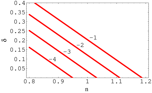
Figure 1: Plot of the COBE normalization condition for $\sigma_{i}=1$, $f(1)=0.33$, $m=10^{10}$ GeV, $k_{1}/k_{s}=k_{1}/k_{\rm eq}\simeq 10^{27}(H_{1}/M_{\rm P})^{1/2}(m/M_{\rm P})^{1/3}$, and for various values of the inflation scale $H_{1}$. The four curves correspond, from left to right respectively, to $\log(H_{1}/M_{\rm P})=-4,-3,-2,-1$.

We conclude that, in the context of the pre-big bang scenario, a “curvaton” model based on the Kalb–Ramond axion is able to produce the adiabatic curvature perturbation needed to explain the observed large-scale anisotropies. The simplest, minimal model of pre-big bang inflation seems to prefer blue spectra. A strictly scale-invariant (or even slightly red, $n<1$) spectrum is not excluded but requires, for normalization purposes, non-minimal models of pre-big bang evolution leading to axion fluctuations with a sufficiently steep slope at high frequencies.

References

- [1] J. E. Lidsey, D. Wands and E. J. Copeland, Phys. Rep. 337, 343 (2000).
- [2] M. Gasperini and G. Veneziano, CERN-TH/2002-104, to appear.
- [3] M. Gasperini and G. Veneziano, Phys. Rev. D50, 2519 (1994); R. Brustein, M. Gasperini, M. Giovannini, V. Mukhanov and G. Veneziano, Phys. Rev. D51, 6744 (1995).
- [4] G. F. Smooth et al., Astrophys. J. 396, 1 (1992); C. L. Bennet et al., Astrophys. J. 430, 423 (1994).
- [5] P. de Bernardis et al., Nature 404, 955 (2000); S. Hanay et al., Astrophys. Lett. 545, 5 (2000).
- [6] F. Finelli and R. Brandenberger, hep-th/0112249; R. Durrer and F. Vernizzi, hep-ph/0203275.
- [7] M. B. Green, J. H. Schwarz and E. Witten, Superstring Theory (Cambridge Univ. Press, Cambridge, 1987).
- [8] E. J. Copeland, R. Easther and D. Wands, Phys. Rev. D56, 874 (1997); E. J. Copeland, J. E. Lidsey and D. Wands, Nucl. Phys. B506, 407 (1997).
- [9] R. Durrer, M. Gasperini, M. Sakellariadou and G. Veneziano, Phys. Lett. B436, 66 (1998).
- [10] R. Durrer, M. Gasperini, M. Sakellariadou and G. Veneziano, Phys. Rev. D59, 43511 (1999).
- [11] R. Durrer, Phys. Rev. D42, 2533 (1990).
- [12] M. Gasperini and G. Veneziano, Phys. Rev. D59, 43503 (1999).
- [13] A. Melchiorri, F. Vernizzi, R. Durrer and G. Veneziano, Phys. Rev. Lett. 83, 4464 (1999); F. Vernizzi, A. Melchiorri and R. Durrer, Phys. Rev. D63, 063501 (2001).
- [14] K. Enqvist and M. S. Sloth, Nucl. Phys. B626, 395 (2002).
- [15] D. H. Lyth and D. Wands, Phys. Lett. B524, 5 (2002).
- [16] T. Moroi and T. Takahashi, Phys. Lett. B522, 215 (2001); T. Moroi and T. Takahashi, hep-ph/0206026.
- [17] N. Bartolo and A. R. Liddle, astro-ph/0203076.
- [18] A. Notari and A. Riotto, hep-th/0205019.
- [19] S. Mollerach, Phys. Rev. D42, 313 (1990).
- [20] V. Bozza, M. Gasperini, M. Giovannini and G. Veneziano, to appear.
- [21] V. F. Mukhanov, H. A. Feldman and R. H. Brandenberger, Phys. Rep. 215, 203 (1992).
- [22] J. Ellis, D. V. Nanopoulos and M. Quiros, Phys. Lett. B174, 176 (1986); J. Ellis, C. Tsamish and M. Voloshin, Phys. Lett. B194, 291 (1987).
- [23] M. Abramowitz and I. A. Stegun, Handbook of mathematical functions (Dover, New York, 1972).
- [24] W. Hu and N. Sugiyama, Astrophys. J. 444, 489 (1995); ibid. 471, 542 (1996); Phys. Rev. D51, 2599 (1995).
- [25] S. Weinberg, Phys. Rev. D64, 123511 and 123512 (2001).
- [26] H. Kodama and M. Sasaki, Int. J. Mod. Phys. A1, 265 (1986).
- [27] R. Durrer, astro-ph/0109522.
- [28] A. J. Banday et al., Astrophys. J. 475, 393 (1997).
- [29] C. L. Bennet et al., Astrophys. Lett. 464, L1 (1996).
- [30] G. Veneziano, hep-th/0110129.
- [31] P. de Bernardis et al., Astrophys. J. 564, 559 (2002).
- [32] X. Wang, M. Tegmark and M. Zaldarriaga, Phys. Rev. D65, 123001 (2002).