Effects of Squark Processes on the
Axino CDM Abundance

Abstract:

We investigate the role of an effective dimension-$4$ axino-quark-squark coupling in the thermal processes producing stable cold axino relics in the early Universe. We find that, while the induced squark and quark scattering processes are always negligible, squark decays become important in the case of low reheat temperature and large gluino mass. The effect can tighten the bounds on the scenario from the requirement that cold dark matter axinos do not overclose the Universe.

1 Introduction

The nature of the dark matter (DM) in the Universe remains one of the most challenging problems in cosmology. Numerous candidates for DM have been proposed in the literature. One of the most popular candidates in the context of supersymmetric theories with $R$-parity conservation is the lightest supersymmetric particle (LSP). Such a candidate has usually been studied in the framework of supersymmetric extensions of the Standard Model, such as the Minimal Supersymmetric Standard Model (MSSM) [1] or its constrained version (CMSSM) [2]. In these models, the LSP is often the lightest neutralino, i.e. a linear combination of the fermionic superpartners of neutral gauge and Higgs bosons. The interactions of the neutralino are weak, and its number density at decoupling is therefore often of the required order of magnitude, which makes it an excellent candidate for the WIMP (Weakly Interacting Massive Particle) [3].

The case of the neutralino WIMP is very appealing and puts strong bounds on SUSY masses and parameters [1, 2], but it is certainly not a unique one. One should not forget that very different possibilities can arise in other well-motivated extensions of the Standard Model. For example, in the framework of supergravity there arises the gravitino, the SUSY partner of the graviton. The gravitino has long been known to be a potential candidate for DM [4]. A number of more speculative possibilities, stemming from, for example, string theories, have also been proposed.

The aim of this paper is to investigate another well-motivated scenario, in which the LSP is the axino. Such a particle is present in SUSY models that incorporate the Peccei-Quinn (PQ) solution to the strong CP problem. The PQ global $U(1)$ symmetry [5] was introduced more than 20 years ago to solve the strong CP problem, and still remains the most elegant solution, especially since lattice results seem to disfavor the possibility of a massless up-quark [6]. The axino does not belong to the usual MSSM spectrum, but, as a fermionic superpartner of the axion [7, 8], is much more weakly interacting. Similarly to the case of the axion, the couplings of the axino to “ordinary” matter (below simply referred to as “matter”) are suppressed by the Peccei-Quinn scale $f_{a}\sim 10^{11}\,\mbox{GeV}$, thus the axino remains invisible to present experimental searches.

A stable relic axino has been shown to be an attractive candidate for either warm [9, 10, 11, 12] or, preferably, cold dark matter (CDM) [12, 13]. An underlying assumption is that a primordial axino population was washed away by an earlier inflationary period. Axinos can then again be produced in large numbers through several possible mechanisms. One efficient way is through thermal production (TP); this proceeds via thermal scatterings involving, e.g., gluinos (and their decays) in the primordial plasma [10, 12], in close analogy with gravitino production [4]. Another one is non-thermal production (NTP): an example of this being an out-of-equilibrium decay of the next-to-lightest particle (NLSP) [9, 13]. A number of papers have investigated cosmological properties of axinos as warm [9, 11, 14] or cold relics [15, 16].

In a recent extensive analysis [12], the role of the effective dimension-5 gluino-gluon-axino interaction was examined in the production of stable axinos as relics in the Universe. At high reheat temperatures $T_{R}$ (much larger than squark/gluino masses but still $T_{R}\ll f_{a}$ in order not to restore the PQ symmetry), the thermal production of axinos via scattering processes was shown to be dominant. This allows one to place strong bounds on the reheat temperature as a function of the axino mass by imposing the constraint $\Omega_{\tilde{a}}h^{2}\mathrel{\hbox to0.0pt{\lower 4.0pt\hbox{\hskip 1.0pt$\sim$}\hss}\raise 1.0pt\hbox{$<$}}1$. At lower $T_{R}$, gluino decays in the thermal plasma and, at $T_{R}\ll m_{\tilde{g}}$, non-thermal production of axinos were shown to become more important.

The scope of this paper is to supplement the analysis in [13, 12] by investigating the thermal production of axinos involving the dimension-4 squark-quark-axino interaction. The effective vertex for this interaction arises at a one loop order in an effective theory but we find it to be enhanced by the gluino mass. For this reason, we argue that squark decays cannot be neglected in a computation of the axino abundance, especially in the case of a heavy gluino.

The paper is organized as follows. In Sec. 2 we briefly review axion models. In Sec. 3 we introduce the effective squark-quark-axino vertex which is then computed in Sec. 4. The formalism for the thermal production of axinos is reviewed in Sec. 5 and applied to two- and three-body squark decays in Sec. 6 and to scattering of quarks and squarks in Sec. 7. We present our numerical analysis in Sec. 8 and conclude in Sec. 9.

2 Axion models

In the PQ scenario, a complex scalar field is introduced, which breaks the global $U(1)_{PQ}$ at a high scale and whose Goldstone boson component, the axion, plays the role of a dynamical $\theta_{QCD}$ relaxing at the origin after the QCD phase transition. In fact, after the chiral symmetry breaking, the axion acquires a tiny mass from instanton effects [17].

Two classes of models implementing the PQ mechanism are usually studied in the literature: the KSVZ-type (hadronic) axion models (KSVZ) [18] and the DFSZ-type models [19]. In the first case, the SM particles are not charged under $U(1)_{PQ}$, while in the second they are. For this reason, different axion interactions are present in the two approaches.

In supersymmetric extensions of axion models the axion field is promoted to a chiral multiplet [20] which contains not only the pseudoscalar axion, but also a scalar, the saxion, and their fermionic superpartner, the axino. An interesting feature of such supersymmetric models is that the PQ global symmetry is enlarged to a complex $U(1)$, which ensures that the whole axion multiplet is massless and degenerate [21], as long as supersymmetry and the chiral symmetry are unbroken. If supersymmetry is broken at low energies, as is required to explain the large hierarchy between the electroweak and the Planck scale, we can assume that this degeneracy is not strongly lifted, and consider a model in which the axion multiplet is the only additional low-energy degree of freedom compared to those already contained in the MSSM.

The breaking of supersymmetry reduces the complex $U(1)$ to the usual $U(1)_{PQ}$ and generates a soft mass for the saxion [22], while the axion remains protected by the surviving $U(1)_{PQ}$. For the axino different scenarios can arise, strongly dependent on the model and the particle content [21, 23]. In general, the axino, being a component of a chiral multiplet, does not acquire a tree-level Majorana soft mass term. However, a Dirac mass term may arise which will lead to mixing with the neutral heavy states in the PQ sector and the MSSM neutral higgsinos, giving rise to an enlarged neutralino mass matrix at low energy.

On the other hand, if the mixing of the neutralino-axino is very tiny, or absent, an axino nearly massless mass eigenstate survives at the tree level (see [21, 23, 12]). Particularly interesting is the case in which a Majorana mass for the axino is generated at one loop [24, 25], falling naturally in the range of a few tens of GeV, often below the present bounds on the neutralino. This bound obviously does not apply to an axino state due to its suppressed interactions with SM particles.

Phenomenologically, an appealing scenario arises: the LSP axino remains unobserved due to the very tiny couplings of the axion multiplet with matter, and does not spoil the precision measurements of the SM, but still plays a key role in the cosmological evolution of the Universe.

3 The interactions of the KSVZ axino

In this paper we consider mainly an axino of the KSVZ type; our final results are expected to be similar to the case of the DFSZ axino, and we will comment on the differences below.

In the KSVZ, or hadronic, axion models, the axion multiplet (and therefore also the axino) does not couple directly with ordinary matter, instead its interactions with matter are suppressed not only by the PQ scale, but also by loop factors.

A simple example for the superpotential for a KSVZ axion multiplet is [26]

$$W=\lambda\Phi Q\bar{Q}+S(f_{a}^{2}-\Phi\bar{\Phi})$$ (1)

where $Q,\bar{Q}$ are PQ-charged, heavy colored triplet states, $\Phi$ and $\bar{\Phi}$ are PQ-charged SM singlets, while $S$ is a singlet with respect to both the SM and PQ symmetries.

The axion multiplet is in this simple case contained in $\Phi$ and $\bar{\Phi}$: writing their scalar and fermionic part in terms of the axion multiplet ${\cal A}=(A,\tilde{a})$ and another complex scalar and fermion pair $(B,\psi)$, we obtain respectively

$$\Phi\rightarrow\left(f_{a}\exp\left[(B+A)/(\sqrt{2}f_{a})\right],(\psi+\tilde{a})/\sqrt{2}\right)$$

$$\bar{\Phi}\rightarrow\left(f_{a}\exp\left[(B-A)/(\sqrt{2}f_{a})\right],(\psi-\tilde{a})/\sqrt{2}\right).$$ (2)

From the superpotential (1), we see that in the supersymmetric vacuum with $\langle\Phi\bar{\Phi}\rangle=f_{a}^{2}$, only the axion multiplet remains massless and all the other states acquire a mass of the order of $f_{a}$. Note also that no direct coupling between the axion and the MSSM fields is present in (1). However, axino couplings to MSSM fields do arise in the low energy effective action and will be derived below.

Figure 1: The two Feynman diagrams contributing to the gluino-gluon-axino interaction. The extra quark $Q$ and squark $\widetilde{Q}$ states are all very heavy, $m_{Q,\widetilde{Q}}\sim f_{a}$, which allows one to contract the loops to an effective “tree-level” gluino-gluon-axino vertex.

The interaction of the axino with gluons and gluinos proceeds via the anomaly one-loop diagrams shown in Fig. 1. After integrating out the heavy KSVZ quarks $Q$ and squarks $\tilde{Q}$ ($m_{Q,\widetilde{Q}}\sim f_{a}$), we are left with a single effective gluino-gluon-axino dimension-5 interaction term in the Lagrangian

$${\cal L}_{\tilde{a}g\tilde{g}}=\frac{\alpha_{s}}{8\pi(f_{a}/N)}\bar{\widetilde{a}}\gamma_{5}\sigma^{\mu\nu}\widetilde{g}^{b}G^{b}_{\mu\nu}$$ (3)

where $b=1,\ldots,8$, $\widetilde{g}$ is the gluino and $G$ is the strength of the gluon field, while $N$ is the number of flavors of quarks with the Peccei-Quinn charge, and is equal to $1$ ($6$) in KSVZ (DFSZ) models. For the remainder of this paper, we understand $f_{a}$ to mean $f_{a}/N$.

The coupling (3) can also be obtained by supersymmetrizing the axion-gluon-gluon interaction, which corresponds to adding the following Wess-Zumino term to the MSSM superpotential:

$$W_{WZ}={\alpha_{s}\over 2\sqrt{2}\pi f_{a}}{\cal A}\;Tr\left[W_{\alpha}W^{\alpha}\right],$$ (4)

where ${\cal A}$ is the axion multiplet, $W_{\alpha}$ the vector multiplet containing the gluon, and the trace sums over color indices. An interesting characteristic is that the coupling above is only determined by the QCD anomaly of the heavy states and is not subject to renormalization [27] or model dependence.

In an analogous way, Wess-Zumino terms can arise also for the other gauge interactions, depending on the charge of the heavy quark multiplet; at high energy, when all leptons can be considered massless, such interactions can be rotated into the $U(1)_{Y}$ direction [12] and we are left to consider only the term

$$W_{WZ}={\alpha_{Y}C_{aYY}\over 4\sqrt{2}\pi f_{a}}{\cal A}\;B_{\alpha}B^{\alpha}\,,$$ (5)

where $B_{\alpha}$ is the hypercharge vector multiplet and $C_{aYY}$ is a model-dependent factor [28], which vanishes if the heavy KSVZ quarks are electrically neutral. If they have electric charge $e_{Q}=-1/3,+2/3$, then $C_{aYY}=2/3,8/3$. This superpotential term leads to the addition of the following effective dimension-5 interaction term to the low-energy Lagrangian

$${\cal L}_{\tilde{a}B\tilde{B}}=\frac{\alpha_{Y}C_{aYY}}{8\pi f_{a}}\bar{\widetilde{a}}\gamma_{5}\sigma^{\mu\nu}\tilde{B}B_{\mu\nu}$$ (6)

Cosmological implications of the effective axino-gauge boson-gaugino operators (3) and  (6) have been extensively studied in [12].

However, in addition there arises the effective dimension-4 coupling of the axino to quarks and squarks when we integrate out the heavy states:

$${\cal L}_{\tilde{a}q\tilde{q}}=g_{eff}^{L/R}\;\widetilde{q}^{L/R}_{j}\,\bar{q}_{j}P_{R/L}\gamma^{5}\widetilde{a}.$$ (7)

We find that this effective coupling, which arises at two-loop level in KSVZ models (and therefore at a one-loop level in the effective theory valid much below $f_{a}$), can play an important role in the thermal production of axinos.

Instead of undertaking the complicated task of a full computation of $g_{eff}^{L/R}$ in the renormalizable theory, which would give a result strongly dependent on the unknown parameters of the axion superpotential anyway, our strategy is to resort to the expedient of estimating the coupling via an effective theory, given by the MSSM plus the interaction in Eq. (3). That is to say, we compute the two one-loop diagrams in Fig. 2, and use our result to define an effective squark-quark-axino vertex in the low energy Lagrangian. We are then able to study the effects of the coupling on the axino abundance.

Figure 2: The Feynman diagrams contributing to the squark-quark-axino interaction. The thick dot denotes the effective gluino-gluon-axino vertex of Fig. 1.

Let us now mention the situation for the DFSZ models. In that case, the axino can mix with all the other neutralinos through the coupling which generates the Higgs $\mu$ term, and due to this mixing the coupling in Eq. (7) arises at tree level. Since the mixing is strongly suppressed by at least the ratio of the electroweak to the PQ scale, $v_{EW}/f_{a}$, and since we consider the case when an axino-like light state remains in the spectrum, we do not expect the full DFSZ result for $g_{eff}^{L/R}$ to be much larger than our result for the KSVZ case.

In general, the effective coupling to a quark and a squark could be enhanced for the DFSZ axino, but is not expected to be suppressed, unless there are very unlikely cancellations between diagrams. Therefore, the upper bounds on the reheat temperature we obtain for the KSVZ case are also conservative bounds for the DFSZ model.

4 The effective squark-quark-axino vertex

We now proceed to compute the effective dimension-4 squark-quark-axino interaction defined by the two diagrams in Fig. 2. The corresponding amplitudes for an axino $\widetilde{a}$ with momentum $k_{1}$, a quark $q$ with momentum $k_{2}$ and a squark $\widetilde{q}^{L/R}$ with momentum $k_{1}+k_{2}$, are given by:

$${\cal A}_{1}^{L/R} = \pm{4\sqrt{2}\over 3}{\alpha^{2}_{s}\over f_{a}}\,\,\bar{u}_{q}(k_{2})I_{1}^{L/R}\gamma^{5}v_{\tilde{a}}(k_{1})$$ (8)

$${\cal A}_{2}^{L/R} = \mp{8\sqrt{2}\over 3}{\alpha^{2}_{s}\over f_{a}}\,\,\bar{u}_{q}(k_{2})I_{2}^{L/R}\gamma^{5}v_{\tilde{a}}(k_{1})$$ (9)

where summation over color has been performed, the upper/lower signs refer to left- and right-handed (s)quarks respectively, and $I^{L/R}$’s come from loop integrations. We have suppressed the flavor index since the amplitudes are diagonal in flavor space.

The integral of $I^{L/R}_{1}$ is logarithmically divergent; in the full renormalizable KSVZ model (with broken supersymmetry), such a divergence would be taken care of by a counterterm and reabsorbed in the parameters of the Lagrangian. Rather than perform the full renormalization, we instead keep the dependence on the UV cut-off $f_{a}$. This procedure is justified by the fact that we are working in the context of a non-renormalizable effective theory, valid only below $f_{a}$. At higher scales, all the heavy degrees of freedom become dynamical. With this method, we are absorbing all our ignorance about the high energy theory into one single parameter, the “effective” PQ scale $f_{a}$. This allows us to perform a model-independent analysis of the implications of the effective coupling.

We have performed the loop integration using the usual methods, based on the Feynman parameterization. To lowest order in $1/f_{a}$, for $m_{q_{j}}\rightarrow 0$ and assuming that the axino mass is much smaller than the gluino mass $m_{\tilde{g}}$, we obtain

$$I_{1}^{L/R} = {-3im_{\tilde{g}}\over 8\pi^{2}}P_{R/L}\left[\log\left({f_{a}\over m_{\tilde{g}}}\right)+{1\over 3}-{1\over 3}\left(1-{m^{2}_{\tilde{g}}\over 2k_{1}\cdot k_{2}}\right)\log\left(1-{2k_{1}\cdot k_{2}\over m^{2}_{\tilde{g}}}\right)\right]$$ (10)

$$I_{2}^{L/R} = {-3im_{\tilde{g}}\over 8\pi^{2}}P_{R/L}\left[-{1\over 3}+{\pi^{2}\over 18}{m_{\tilde{g}}^{2}\over 2k_{1}\cdot k_{2}}-{1\over 3}{m^{2}_{\tilde{g}}\over 2k_{1}\cdot k_{2}}\textrm{Li}_{2}\left(1-{2k_{1}\cdot k_{2}\over m^{2}_{\tilde{g}}}\right)\right.$$ (11)

$$\left.~{}~{}~{}~{}~{}~{}~{}~{}~{}~{}~{}~{}~{}~{}~{}~{}~{}~{}~{}+{1\over 6}\left(1+{m_{\tilde{g}}^{2}\over m_{\tilde{g}}^{2}-2k_{1}\cdot k_{2}}\right)\log\left({2k_{1}\cdot k_{2}\over m^{2}_{\tilde{g}}}\right)\right].$$

Due to the chiral structure of the loop, the result is proportional to the mass of the internal fermions.

Using these expressions and the definition of $g_{eff}^{L/R}$ in (7), we arrive at

$$g_{eff}^{L/R} = \mp i{4\sqrt{2}\over 3}{\alpha_{s}^{2}\over f_{a}}\left(I_{1}^{L/R}-2I_{2}^{L/R}\right)$$ (12)

$$\simeq \mp{\alpha_{s}^{2}\over\sqrt{2}\pi^{2}}{m_{\tilde{g}}\over f_{a}}\log\left({f_{a}\over m_{\tilde{g}}}\right),$$ (13)

Note that the dominant contribution comes from the logarithmically divergent part. However, as in all supersymmetric theories the dependence on the cut-off is weak. Also, the limit of large $f_{a}$ is perfectly well-defined and the coupling vanishes in the decoupling limit, when $f_{a}\rightarrow+\infty$. Another important point is that the coupling depends on a single unknown parameter, the ratio $m_{\tilde{g}}/f_{a}$: therefore in the following we keep $f_{a}=10^{11}\,\mbox{GeV}$ fixed, and vary the value of the gluino mass to explore the parameter space.

Secondly, the effective vertex is proportional to the gluino mass and tends to zero in the limit of exact supersymmetry and massless quarks; this can be easily understood by considering that for massless quarks the whole axion multiplet decouples from the low energy Lagrangian [8]. When the chiral symmetry is broken, a term proportional to the quark mass survives, giving an axino-quark-squark coupling of the same type as the standard axion-quark-quark coupling.

However, in the case of broken supersymmetry a new contribution to the coupling arises from the gluino mass and dominates for all light quarks. For the top quark, the term proportional to $m_{t}$ could be important for small gluino masses. We neglect this term here since it would not change our results substantially.

It is also worth mentioning that the full expression above contains, in the limit of negligible final state masses, terms proportional to $\log(1-m_{\tilde{q}}^{2}/m_{\tilde{g}}^{2})$. Therefore $g_{eff}^{L/R}$ contains an imaginary component if $m_{\tilde{q}}>m_{\tilde{g}}$. This imaginary piece corresponds to the “cut” loop diagram, in which the intermediate gluino and quark are real. Since this contribution is already included when considering the squark decay into a gluino and a quark, we keep only the real part of $g_{eff}^{L/R}$ to avoid double counting.

5 Thermal production of axinos

For reheat temperatures below $f_{a}$, the axinos are not in thermal equilibrium with the MSSM particles. Assuming that any primordial axino population was completely diluted away during an inflationary stage, the present axino density has been generated after the end of inflation, since the epoch of reheating/preheating. Two different production mechanisms are possible: thermal production, TP, in which axinos are produced via thermal processes in the primordial plasma; and non-thermal production, NTP, which is independent of the presence of the thermal bath. An example of the latter is the decay of the neutralino NLSP after it freezes out, as considered in [13]. In this case the final number density is related only to the density and lifetime of the initial neutralino population.

In the case of TP, on the other hand, the axino number density $n_{\tilde{a}}$ depends on the species and processes present in the plasma, and can be obtained by integrating the Boltzmann equation with the appropriate collision integral. Fortunately, since the number density of axinos is well below the equilibrium one for $T_{R}\ll f_{a}$, we can neglect the inverse processes, which are suppressed by $n_{\tilde{a}}$, and we have:

$$\frac{d\,n_{\tilde{a}}}{d\,t}+3Hn_{\tilde{a}}=\sum_{i}\langle\Gamma(i\rightarrow\widetilde{a}+\cdots)\rangle n_{i}+\sum_{i,j}\langle\sigma(i+j\rightarrow\widetilde{a}+\cdots)v_{\rm rel}\rangle n_{i}n_{j},$$ (14)

where the Hubble parameter, $H$, can be given as a function of the temperature by $H(T)=\left[\left(\pi^{2}g_{\ast}\right)/\left(90M_{\rm P}^{2}\right)\right]^{1/2}\;T^{2}$ in the radiation-dominated era, with $g_{*}$ counting the number of effective massless degrees of freedom and $M_{\rm P}$ denoting the reduced Planck mass, $M_{\rm P}=2.4\times 10^{18}\,\mbox{GeV}$.

The first term on the r.h.s. takes into account all the decay channels of the $i$th particle with one axino in the final state, and $\langle\Gamma(i\rightarrow\widetilde{a}+\cdots)\rangle$ is the thermally averaged decay width for the process. The second term corresponds to axino production via 2 to 2 particle scatterings, with $\sigma(i+j\rightarrow\widetilde{a}+\cdots)$ denoting the cross-section for particles $i,j$ scattering into final states involving axinos and $v_{\rm rel}$ the relative velocity. Averaging over initial spins and summing over final spins is understood.

In order to solve Eq. (14), it is convenient to separate the two contributions and introduce the axino TP yield as [12]

$$Y^{\rm TP}_{\tilde{a}} = \frac{n_{\tilde{a}}^{\rm TP}}{s}$$ (15)

$$= \sum_{i}Y^{\rm dec}_{i}+\sum_{i,j}Y^{\rm scat}_{i,j}\,,$$

where $s=(2\pi^{2}/45)g_{s\ast}T^{3}$ is the entropy density, and normally $g_{s\ast}=g_{\ast}$ in the early Universe.

Moreover, by changing variables from the cosmic time $t$ to the temperature $T$, we can write the two solutions of the Boltzmann differential equation easily in integral form:

$$Y^{\rm dec}_{i}(T_{0}) = \int_{T_{0}}^{T_{R}}dT\,\frac{\langle\Gamma(i\rightarrow\widetilde{a}+\cdots)\rangle n_{i}}{sHT}$$ (16)

$$Y^{\rm scat}_{i,j}(T_{0}) = \int_{T_{0}}^{T_{R}}dT\,\frac{\langle\sigma(i+j\rightarrow\widetilde{a}+\cdots)\rangle n_{i}n_{j}}{sHT}.$$ (17)

where we have considered the evolution from the reheating temperature after inflation, $T_{R}$, down to the present temperature $T_{0}$. Full expressions for $Y^{\rm dec}_{i}$ and $Y^{\rm scat}_{i,j}$ can be found in [29].

In the following we consider the axino yield generated by the effective coupling in Eq. (7). We compute the contribution due to squark decays and estimate the additional contribution to quark scattering. The axino number density arising from gaugino decays and scattering via the dimension-$5$ gluino-gluon-axino operator in (3) was computed in [12].

6 Squark decay

The squark can decay into axinos in two different ways: via $g_{eff}^{L/R}$ into a two-body final state of an axino and a quark, or via an exchange of an intermediate gluino/neutralino and the anomalous couplings into a three-body final state of an axino, a quark and a gluon/photon. As we will see, the first one will play an important role while the second will always remain subdominant.

6.1 Two-body squark decay

The process involves the diagrams shown in Fig. 2. The width for this decay of both left- and right-handed squarks is given by

$$\Gamma_{\tilde{q}}^{2body} = {(g_{eff})^{2}\over 16\pi}m_{\tilde{q}}$$

$$= {\alpha_{s}^{4}\over(2\pi)^{5}}m_{\tilde{q}}\left[{m_{\tilde{g}}\over f_{a}}\log\left({f_{a}\over m_{\tilde{g}}}\right)\right]^{2}$$

$$\simeq \left(2.6\times 10^{-6}\,\textrm{sec}\right)^{-1}\left({m_{\tilde{q}}\over 500\,\mbox{GeV}}\right)\left[\left({m_{\tilde{g}}\over 1\,\mbox{TeV}}\right)\left(1-0.05\log\left({m_{\tilde{g}}\over{{1\,\mbox{TeV}}}}\right)\right)\right]^{2}\!,$$

where in the last line we have taken the default value of $f_{a}=10^{11}\,\mbox{GeV}$. This process is suppressed by a large power of the strong coupling and by loop factors, but it can still be sizable for large gluino mass, or equivalently for smaller $f_{a}$.

6.2 Three-body decay

At an effective tree-level, the squark will also decay into an axino, a quark and a gluon, as illustrated in Fig. 3.

Figure 3: Three-body decay of a squark into an axino, a quark and a gluon. The thick dot denotes the effective gluino-gluon-axino vertex of Fig. 1.

The decay rate for this process in the case of large gluino mass $m_{\tilde{g}}>m_{\tilde{q}}$ and negligible final state masses is:

$$\Gamma_{\tilde{q}}^{3body}={4\alpha_{s}^{3}\over 3(4\pi)^{4}}{m^{3}_{\tilde{q}}\over f_{a}^{2}}F\left({m_{\tilde{g}}^{2}\over m_{\tilde{q}}^{2}}\right)$$ (19)

where we have summed over the color indices of the final state gluon and quark and where

$$F(x)={1\over 6}-{13x\over 4}+{7x^{2}\over 2}+{x\over 4}\left(1-x\right)\left(3-7x\right)\log\left[{(1-x)^{2}\over x^{2}}\right].$$ (20)

In the limit $m_{\tilde{g}}\gg m_{\tilde{q}}$, (19) reduces to

$$\Gamma_{\tilde{q}}^{3body}={\alpha_{s}^{3}\over 18(4\pi)^{4}}{m^{5}_{\tilde{q}}\over m^{2}_{\tilde{g}}f_{a}^{2}}~{}\left[1+O\left({m_{\tilde{q}}^{2}\over m_{\tilde{g}}^{2}}\right)\right].$$ (21)

Note again that, in our effective theory, the 3-body decay width (19) is proportional to the cube of the mass of the decaying particle. However, in the limit when one can neglect momentum flow in the intermediate states, one recovers in (21) the usual fifth power of mass for a dimension-4 interaction.

Comparing (21) with (6.1) gives

$${\Gamma_{\tilde{q}}^{3body}\over\Gamma_{\tilde{q}}^{2body}}={\pi\over 144\alpha_{s}}\;\left({m_{\tilde{q}}\over m_{\tilde{g}}}\right)^{4}\;\log^{-2}\left(f_{a}/m_{\tilde{g}}\right)\ll 1$$ (22)

The $3$-body decay channel is therefore subdominant for squarks lighter than gluinos. For example, if $m_{\tilde{q}}=500\,\mbox{GeV},m_{\tilde{g}}=1\,\mbox{TeV}$ and $f_{a}=10^{11}\,\mbox{GeV}$, we have

$$\Gamma_{\tilde{q}}^{3body} = \left(4.1\times 10^{-2}\,\textrm{sec}\right)^{-1}\,,$$ (23)

which is suppressed by about four orders of magnitude relative to the two-body decay (6.1).

An analogous decay channel exists with an intermediate neutralino replacing the gluino and a final photon rather than a gluon. Taking the neutralino to be a bino [30], the decay of each color of squark into a quark, an axino and a photon is given by:

$$\Gamma_{\tilde{q}}^{L/R}={\alpha_{em}^{3}\over(4\pi)^{4}}~{}\left({C_{aYY}Z^{2}_{11}Y_{\widetilde{q}^{L/R}}\over\cos\theta_{W}}\right)^{2}~{}\left({m^{3}_{\tilde{q}}\over f_{a}^{2}}\right)~{}F\left({m_{\chi}^{2}\over m_{\tilde{q}}^{2}}\right),$$ (24)

where $Y^{2}_{\widetilde{q}^{L/R}}=1/36,4/9,1/9$ for a left-handed squark, a right-handed up-type squark and a right-handed down-type squark, respectively. For $m_{\tilde{q}}=500\,\mbox{GeV},m_{\tilde{g}}=1\,\mbox{TeV}$ and $f_{a}=10^{11}\,\mbox{GeV}$, we have

$$\Gamma_{\tilde{q}}^{L/R}\simeq\left(10\,\textrm{sec}\right)^{-1}\;C_{aYY}^{2}Z^{2}_{11}Y^{2}_{\widetilde{q}^{L/R}}$$ (25)

This is an even smaller contribution than that from the gluino exchange diagram above. Therefore we conclude that three-body decays are not expected to contribute substantially to the axino yield.

Note that we have considered the decays only for the case of intermediate particle heavier than the initial squark. For an intermediate particle lighter than the initial squark, the dominant contribution to the axino production comes from the resonance. This contribution can be factorized into the squark decay to a real neutralino/gluino, and its subsequent decay to an axino and a photon/gluon. This process is already included in the Boltzmann equation in the gaugino/neutralino decay term.

6.3 Yield from the decay of squarks

In general, the thermal average of a decay described by a width $\Gamma$ is given by

$$\langle\Gamma\rangle n_{i}=\Gamma~{}\frac{m_{i}T^{2}}{2\pi^{2}}\int_{m_{i}/T}^{\infty}dx\,\frac{(x^{2}-m_{i}^{2}/T^{2})^{1/2}}{e^{x}\mp 1}$$ (26)

where the $-(+)$ is for decaying boson (fermion). By inserting this expression into (16), one obtains

$$Y^{\rm dec}_{i} = \frac{{\overline{g}}M_{P}\Gamma}{16\pi^{2}m_{i}^{2}}\int_{t_{R}}^{\infty}dt\,\frac{1}{e^{t}\mp 1}\Bigg{[}\Bigg{\{}\frac{\pi}{2}-\textrm{tan}^{-1}\Bigg{(}\frac{t_{R}}{\sqrt{t^{2}-t_{R}^{2}}}\Bigg{)}\Bigg{\}}t^{4}$$ (27)

$$\hskip 57.81621pt+t_{R}(t^{2}-2t_{R}^{2})\sqrt{t^{2}-t_{R}^{2}}~{}\Bigg{]}$$

where $t_{R}=m_{i}/T_{R}$ and ${\overline{g}}=135\sqrt{10}/(2\pi^{3}g_{*}^{3/2})$, for $g_{*}=915/4$ for the MSSM in the early Universe.

In the case $T_{R}>m_{i}$, the integration gives the simple result

$$Y^{\rm dec}_{i}\simeq\frac{3\zeta(5){\overline{g}}M_{P}\Gamma}{4\pi m_{i}^{2}}.$$ (28)

To obtain the axino yield from squark decay, we substitute (6.1) for the decay rate above, and obtain the following expression, valid for $T_{R}>m_{\tilde{q}}$

$$Y_{\tilde{q}}^{dec} = \frac{6\zeta(5)\alpha_{s}^{4}}{(2\pi)^{6}}\,{\overline{g}}\,\left(\frac{M_{P}}{m_{\tilde{q}}}\right)\left[\left(\frac{m_{\tilde{g}}}{f_{a}}\right)\log\left(\frac{f_{a}}{m_{\tilde{g}}}\right)\right]^{2}$$ (29)

$$\simeq 3~{}\left(\frac{m_{\tilde{g}}}{m_{\tilde{q}}}\right)Y_{\tilde{g}}^{dec}\simeq 10^{-8}.$$ (30)

The numerical value corresponds to $m_{\tilde{g}}=m_{\tilde{q}}=1\,\mbox{TeV}$ and $f_{a}=10^{11}\,\mbox{GeV}$. It is clear that squark decay is typically as important as gluino decay in the thermal production of axinos, and can be substantially more important if the squarks are lighter than the gluinos. For $T_{R}$ less than the mass of the decaying sparticle, both yields are Boltzmann suppressed and negligible.

7 Scattering of quarks and squarks

The effective dimension-$4$ squark-quark-axino coupling (12) also gives new contributions to some of the scattering axino production processes previously considered in [12] which involved the effective gluino-gluon-axino vertex (3). However, we shall see that such additional contributions will be always subdominant.

Figure 4: Example of dimension-5 contribution to the process $qq\rightarrow\widetilde{q}\widetilde{a}$ (Process I).

As an example and for a conservative estimate, let us consider the scattering of two quarks into a gluino and axino. (This process was called process I in [12].) This process does not contain sparticles in the initial state and is therefore never Boltzmann-suppressed by the number density of the initial particles. Therefore process I is expected to be one of the dominant contributions to the axino yield from dimension-4 interactions at low temperatures.

As we will show below, the dimension-$5$ diagrams that contribute to the scattering process, illustrated in Fig. 4, are of order $g_{s}^{3}$ [12]. The two dimension-$4$ diagrams that contribute are of order $g_{s}^{5}$. They are shown in Fig. 5, where the shaded squares denote the effective 1-loop squark-quark-axino vertices given in Fig. 2. Although these two diagrams are suppressed by $g_{s}^{2}$ relative to the dimension-$5$ contributions, the enhancement through the large logarithm and the gluino mass present in $g_{eff}^{L/R}$ partially compensates for it.

Generalizing the cross section due to the dimension-$5$ coupling computed in Ref. [12] by including a full dependence on the gluino mass, we find that

$$\sigma_{I,5}={\alpha_{s}^{3}\over 72\pi^{2}f_{a}^{2}}\,\left[1-3\left({m_{\tilde{g}}^{2}\over s}\right)^{2}+2\left({m_{\tilde{g}}^{2}\over s}\right)^{3}\right],$$ (31)

where the eight gluino species in the final state have been summed over, and the six flavors of quark in the initial state have been averaged over.

The combined contribution from the two dimension-$4$ channels is

$$\sigma_{I,4}=\frac{2\alpha_{s}(g_{eff}^{L/R})^{2}}{3s^{2}}\left[\frac{(s-m_{\tilde{g}}^{2})\left[s-2(m_{\tilde{g}}^{2}-m_{\tilde{q}}^{2})\right]}{s+m_{\tilde{q}}^{2}-m_{\tilde{g}}^{2}}-(2m_{\tilde{q}}^{2}-m_{\tilde{g}}^{2})\log\left(\frac{s+m_{\tilde{q}}^{2}-m_{\tilde{g}}^{2}}{m_{\tilde{q}}^{2}}\right)\right]$$ (32)

and is proportional to $\alpha_{s}^{5}$. The two squarks corresponding to each quark and the eight gluino species have been summed over in this expression, while we averaged over the initial flavor.

Figure 5: Dimension-4 contributions to Process I.

Interference between the dimension-$4$ $t$ and $u$ channels gives a contribution proportional to $m_{\tilde{a}}$, which is neglected here.

There is also a contribution to the cross-section from interference between dimension-$4$ and dimension-$5$ diagrams, which is of order $\alpha_{s}^{4}$. Giving the $L$ squarks (${\widetilde{q}}_{L}$) a common mass $m_{L}$ and the $R$ squarks (${\widetilde{q}}_{R}$) a common mass $m_{R}$, this 4/5 interference term can be written as

$$\sigma_{I,4/5}=\frac{\sqrt{2}\,\alpha_{s}^{2}\,|g^{L/R}_{eff}|}{3\pi f_{a}}\left(\frac{m_{\tilde{g}}}{s^{2}}\right)\left[m_{L}^{2}\,\log\left(\frac{s+m_{L}^{2}-m_{\tilde{g}}^{2}}{m_{L}^{2}}\right)-m_{R}^{2}\,\log\left(\frac{s+m_{R}^{2}-m_{\tilde{g}}^{2}}{m_{R}^{2}}\right)\right]$$ (33)

Note that the contributions from the $L$ and $R$ squarks cancel in the limit $m_{L}=m_{R}$ thanks to the opposite sign of the coupling $g^{L/R}_{eff}$.

7.1 Yield from dimension-$4$ scattering processes

We numerically computed the axino yield using an estimate of dimension-4 contribution to Process I derived above, and we found it to be negligible compared to the dimension-5 part for any reheat temperature.

To illustrate this analytically, let us consider the following simplified example. In the limit $m_{\tilde{q}}=m_{\tilde{g}}=m$, the contribution to the Process I cross-section from the dimension-$4$ channel is

$$\sigma_{I,4}=\frac{2\alpha_{s}(g_{eff}^{L/R})^{2}}{3s^{2}}\left[s-m^{2}-m^{2}\log\left(\frac{s}{m^{2}}\right)\right]$$ (34)

To calculate the yield we expand around $m/T_{R}=0$. After summing over the four possible combinations of the initial spins, the six quark species and the three colors, and multiplying by a number density factor $3/4$ for each initial fermion, we find

$$Y_{I,4}^{scat} = \frac{9\alpha_{s}(g_{eff}^{L/R})^{2}~{}{\overline{g}}}{8\pi^{3}}~{}\frac{M_{P}}{m}+O\left(\frac{m}{T_{R}}\right)$$

$$\simeq 4.9\times 10^{-10}\left(\frac{\alpha_{s}(m)}{0.11}\right)^{5}\left(\frac{10^{11}\,\mbox{GeV}}{f_{a}}\right)^{2}\left(\frac{m}{1\,\mbox{TeV}}\right).$$

So for $T_{R}$ greater than the masses of the external particles, the axino yields from these dimension-$4$ processes are approximately independent of $T_{R}$. For this reason, in analogy with decay processes, we have used $\alpha_{s}(T=m)$ to take account of the running of the strong coupling.

This is in contrast with what happens for the dimension-$5$ scattering processes. For example, the contribution of the diagram in Fig. 4 to the yield is

$$Y_{I,5}^{scat} \simeq \frac{9\alpha_{s}^{3}~{}{\overline{g}}M_{P}}{16\pi^{6}f_{a}^{2}}T_{R}$$

$$\simeq 3.7\times 10^{-10}\,\left(\frac{\alpha_{s}(T_{R})}{0.11}\right)^{3}\left(\frac{10^{11}\,\mbox{GeV}}{f_{a}}\right)^{2}\,\left(\frac{T_{R}}{1\,\mbox{TeV}}\right)$$

for high reheat temperatures, i.e. $Y_{I,5}\propto T_{R}$. This different behavior is simply due to dimensional reasons: the dimension-$5$ scatterings have cross-sections that are proportional to $1/f_{a}^{2}$ and independent of $s$ at large $s$, while the dimension-$4$ scatterings are characterized by a dimensionless coupling $g_{eff}^{L/R}\propto m_{\tilde{g}}/f_{a}$, and their cross-sections are suppressed by $s^{-1}$ at high energies.

Comparing the two yields, we find that for $T_{R}\gg m$

$$Y_{I,4}^{scat}\simeq 1.3\,Y_{I,5}^{scat}\,\left(\frac{\alpha_{s}(m)}{0.11}\right)^{5}\left(\frac{0.11}{\alpha_{s}(T_{R})}\right)^{3}\left(\frac{m}{T_{R}}\right)$$ (37)

Therefore the contribution to the yield from the two dimension-$4$ diagrams is considerably less than the contribution from the dimension-$5$ diagram already considered for large reheat temperature. As we will see, this is the case also for $T_{R}\simeq m$, when the analytic formulas above are no more valid, since the dimension-$4$ yield reaches the asymptotic value in eq. (7.1) more slowly than the dimension-$5$ one.

Below eq. (33) we noted that the contributions to the cross-section from interference between dimension-$4$ and dimension-$5$ diagrams cancel in the limit $m_{L}=m_{R}$. However, in the case of unequal masses there is a remainder, and therefore a contribution to the yield from $4/5$ interference. We have calculated this contribution in two extreme cases;

$$Y^{scat}_{I,4/5} \simeq ~{}~{}\frac{2}{3}\,Y^{scat}_{I,4}~{}~{}~{}\textrm{if}~{}~{}m_{L}=10\,m_{R}$$ (38)

$$\simeq -\frac{2}{3}\,Y^{scat}_{I,4}~{}~{}~{}\textrm{if}~{}~{}m_{L}=0.1\,m_{R}.$$ (39)

In either case, the magnitude of the effect of the dimension-$4$ diagrams does not become comparable with that of the dimension-$5$ diagrams.

Figure 6: An example of a 2-loop contribution to Process I.

In principle, there are several other diagrams of order $\alpha_{s}^{5}$ that should be computed. For example, the box diagram in Fig. 6 will contribute to the total cross-section of Process I. Such diagrams are also 2-loop in a renormalizable theory (and therefore 1-loop in the effective theory) and as a result suppressed by the same loop factors, but contain no logarithmic divergence and so do not receive the enhancement factor contained in the diagrams considered above. Therefore it seems reasonable to neglect them too.

We conclude that dimension-$4$ scattering diagrams never give a significant contribution to the thermal yield of axinos. The dominant contributions to $Y_{\tilde{a}}^{scat}$ are always those from dimension-$5$ diagrams already considered in [12].

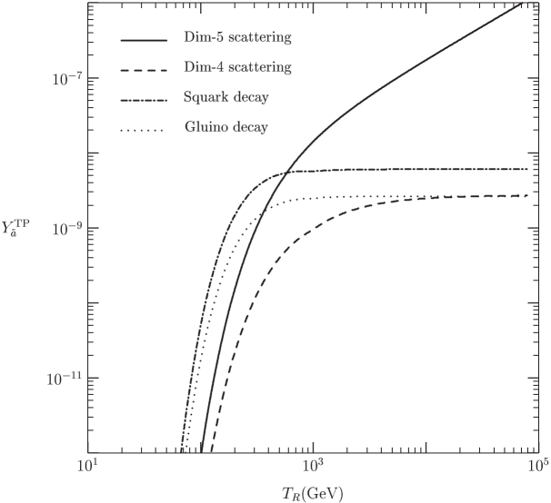
Figure 7: The yield of axinos from thermal production, $Y_{\tilde{a}}^{TP}$, as a function of the reheat temperature $T_{R}$, assuming $f_{a}=10^{11}\,\mbox{GeV}$ and $m_{\tilde{q}}=m_{\tilde{g}}=1\,\mbox{TeV}$.

8 Results

The relative contributions from the processes considered above to the axino abundance are summarized in Fig. 7. The solid line is the yield from dimension-5 scattering processes, while the dashed line is an estimate of dimension-4 scattering processes, computed by multiplying $Y_{I,4}^{scat}$ by seven, which is the number of channels receiving dimension-4 contributions. The figure illustrates that, for equal squark and gluino masses, the yield from dimension-4 scattering processes is negligible for any value of $T_{R}$, whereas the yield from the decay process $\widetilde{q}\to q\widetilde{a}$ can dominate the abundance for $T_{R}\mathrel{\hbox to0.0pt{\lower 4.0pt\hbox{\hskip 1.0pt$\sim$}\hss}\raise 1.0pt\hbox{$<$}}m_{\tilde{q}}$.

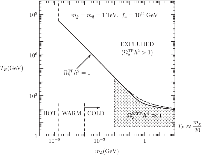
Figure 8: The ($m_{\tilde{a}},T_{R}$) plane, with a bino-like neutralino of mass $100\,\mbox{GeV}$, $m_{\tilde{g}}=m_{\tilde{q}}=1\,\mbox{TeV}$ and $F=10^{11}\,\mbox{GeV}$. The dash-dotted line represents the bound if squark decay is neglected, while the thick line is the full result.

The present fraction of the axino energy density to the critical density $\Omega_{\tilde{a}}$ is given by

$$m_{\tilde{a}}Y_{\tilde{a}}\simeq 0.72\,\mbox{eV}\left(\Omega_{\tilde{a}}h^{2}\over 0.2\right)$$ (40)

where $h$ is the Hubble parameter. Using this relationship, one can redisplay the results of Fig. 7 in the ($m_{\tilde{a}},T_{R}$) plane.

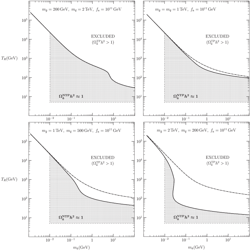
Figure 9: The ($m_{\tilde{a}},T_{R}$) plane, showing the different bounds on the reheat temperature depending on the mass spectrum. For light gluinos, the effective coupling is small and its effect on the axino abundance negligible. For light squarks, axino production through squark decay is so large that most of the allowed parameter space is excluded. Note that, in the figure in the left top panel, the kink at $T_{R}\simeq 10^{2}\,\mbox{GeV}$ is where gluino decays start to dominate scatterings. For large gluino masses the kink is moved to the left and is less pronounced. In the right bottom panel, a similar kink is due instead to the decay of light squarks.

For axinos produced through scatterings and decays of particles in the plasma (TP axinos), eq. (40) gives an upper bound on $T_{R}$ as a function of the axino mass from the requirement $\Omega^{\rm TP}_{\tilde{a}}h^{2}\mathrel{\hbox to0.0pt{\lower 4.0pt\hbox{\hskip 1.0pt$\sim$}\hss}\raise 1.0pt\hbox{$<$}}1$. This bound is depicted by a thick solid line in Fig. 8, for $m_{\tilde{g}}=m_{\tilde{q}}=1\,\mbox{TeV}$ and $F=10^{11}\,\mbox{GeV}$.

At large $T_{R}$, the TP mechanism is dominant and the cosmologically favored region ($0.2\mathrel{\hbox to0.0pt{\lower 4.0pt\hbox{\hskip 1.0pt$\sim$}\hss}\raise 1.0pt\hbox{$<$}}\Omega_{\tilde{a}}h^{2}\mathrel{\hbox to0.0pt{\lower 4.0pt\hbox{\hskip 1.0pt$\sim$}\hss}\raise 1.0pt\hbox{$<$}}0.4$) forms a narrow strip (not indicated in Fig. 8) just below the $\Omega^{\rm TP}_{\tilde{a}}=1$ boundary.

For reheat temperatures less than the mass of the gluinos and squark, non-thermal production of axinos via out of equilibrium neutralino decays can dominate [13, 12]. In that case the neutralinos decay into an axino and a photon or Z well after freeze-out, and the final axino abundance is independent of the reheat temperature, as long as this is high enough for the neutralinos to thermalize before freeze-out. The shaded region below the bound on $T_{R}$, shows where a sufficiently large axino population can be obtained by the decay of a nearly pure bino with mass $m_{\chi}=100\,\mbox{GeV}$. The ranges of $m_{\tilde{a}}$ where axinos are hot/warm/cold dark matter are also shown. More details can be found in [12].

In Fig. 9, an enlarged region of the ($m_{\tilde{a}},T_{R}$) plane is shown for different values of the sparticle masses. The dash-dotted line always represents the bound if squark decay is neglected; clearly, for heavy gluinos, a large region of the parameter space is excluded by including squark decay. This remarkably large effect is due to two factors: for one thing, a light squark remains in thermal equilibrium and can play a role in axino production down to lower temperatures; for another, a large gluino mass enhances the squark decay to axinos.

Note that, as discussed previously, the squark decay rate into axinos is only regulated by the ratio $m_{\tilde{g}}/f_{a}$. Therefore the same effect could be due to a smaller effective PQ scale $f_{a}$ rather than a larger gluino mass.

9 Conclusions

We have computed the effective axino-quark-squark vertex arising in KSVZ axion models through one loop diagrams, and we considered the effects of this interaction for the thermal production of axinos.

As expected by dimensional arguments, we find that the dimension-$4$ scattering diagrams generated by this coupling are negligible with respect to the dimension-$5$ scattering processes already analysed in [12]. On the other hand, the two body decay of a squark to an axino and a quark can be the dominant axino production channel at low reheat temperature, in particular when the squarks are substantially lighter than the gluinos. Our results put tighter constraints on the reheat temperature for the axino CDM scenario, summarized in Fig. 9. For very light squark masses and heavy gluinos, most of the parameter space for NTP axino DM is excluded.

- [1] G. Jungman, M. Kamionkowski and K. Griest, Phys. Rept. 267 (1996) 195.
- [2] For recent results, see, e.g., L. Roszkowski, R. Ruiz de Austri and T. Nihei, J. High Energy Phys. 0108 (2001) 024.
- [3] See, e.g., E.W. Kolb and M.S. Turner, The Early Universe (Addison-Wesley, Redwood City, 1990).
- [4] H. Pagels and J.R. Primack, Phys. Rev. Lett. 48 (1982) 223; S. Weinberg, Phys. Rev. Lett. 48 (1982) 1303; J. Ellis, J.E. Kim and D.V. Nanopoulos, Phys. Lett. B 145 (1984) 181; T. Moroi, H. Murayama and M. Yamaguchi, Phys. Lett. B 303 (1993) 289; M. Bolz, W. Buchmüller, and M. Plümacher, Phys. Lett. B 443 (1998) 209.
- [5] R.D. Peccei and H.R. Quinn, Phys. Rev. Lett. 38 (1977) 1440 and Phys. Rev. D 16 (1977) 1791.
- [6] A.C. Irving, C. McNeile, C. Michael, K.J. Sharkey and H. Wittig, Phys. Lett. B 518 (2001) 243.
- [7] S. Weinberg, Phys. Rev. Lett. 40 (1978) 223; F. Wilczek, Phys. Rev. Lett. 40 (1978) 279.
- [8] J.E. Kim, Phys. Rept. 150 (1987) 1; P. Sikivie, Nucl. Phys. Proc. Suppl. 87 (2000) 41.
- [9] J.E. Kim, A. Masiero and D.V. Nanopoulos, Phys. Lett. B 139 (1984) 346.
- [10] K. Rajagopal, M.S. Turner and F. Wilczek, Nucl. Phys. B 358 (1991) 447.
- [11] S.A. Bonometto, F. Gabbiani and A. Masiero, Phys. Lett. B 222 (433) 1989 and Phys. Rev. D 49 (1994) 3918.
- [12] L. Covi, H.B. Kim, J.E. Kim and L. Roszkowski, J. High Energy Phys. 0105 (2001) 033.
- [13] L. Covi, J.E. Kim and L. Roszkowski, Phys. Rev. Lett. 82 (1999) 4180.
- [14] T. Asaka and T. Yanagida, Phys. Lett. B 494 (297) 2000.
- [15] E.J. Chun, H.B. Kim and D.H. Lyth, Phys. Rev. D 62 (2000) 125001.
- [16] H.B. Kim and J.E. Kim, Phys. Lett. B 527 (2002) 18.
- [17] W.A. Bardeen, S.-H.H. Tye, Phys. Lett. B 74 (1978) 229; V. Baluni, Phys. Rev. D 19 (1979) 2227.
- [18] J.E. Kim, Phys. Rev. Lett. 43 (103) 1979; M.A. Shifman, V.I. Vainstein and V.I. Zakharov, Nucl. Phys. B 166 (1980) 4933.
- [19] M. Dine, W. Fischler and M. Srednicki, Phys. Lett. B 104 (1981) 99; A.P. Zhitnitskii, Sov. J. Nucl. Phys. 31 (1980) 260.
- [20] H.P. Nilles and S. Raby, Nucl. Phys. B 198 (1982) 102; J.E. Kim and H.P. Nilles, Phys. Lett. B 138 (1984) 150.
- [21] E.J. Chun, J.E. Kim and H.P. Nilles, Phys. Lett. B 287 (1992) 123.
- [22] K. Tamvakis and D. Wyler, Phys. Lett. B 112 (1982) 451; J.F. Nieves, Phys. Lett. B 174 (1986) 411.
- [23] E.J. Chun and A. Lukas, Phys. Lett. B 357 (1995) 43.
- [24] P. Moxhay and K. Yamamoto, Phys. Lett. B 151 (1985) 363.
- [25] T. Goto and M. Yamaguchi, Phys. Lett. B 276 (1992) 103.
- [26] J.E. Kim, Phys. Lett. B 136 (1984) 378.
- [27] S. L. Adler and W. A. Bardeen, Phys. Rev. D 49 (1994) 551.
- [28] J.E. Kim, Phys. Rev. D 58 (1998) 055006. See, also, D.B. Kaplan, Nucl. Phys. B 260 (1985) 215; M. Srednicki, Nucl. Phys. B 260 (1985) 689.
- [29] K. Choi, K. Hwang, H.B. Kim and T. Lee, Phys. Lett. B 467 (1999) 211.
- [30] L. Roszkowski, Phys. Lett. B 262 (1991) 59; R.G. Roberts and L. Roszkowski, Phys. Lett. B 309 (1993) 329; G.L. Kane, C. Kolda, L. Roszkowski, and J.D. Wells, Phys. Rev. D 49 (1994) 6173.