SLAC-PUB-9212 UH-511-1000-02 May 2002

Yet Another Extension of the Standard Model: Oases in the Desert?

J. D. Bjorken, S. Pakvasa and S. F. Tuan

Stanford Linear Accelerator Center
Stanford University, Stanford, CA 94309
and University of Hawaii, Honolulu, HI 96822

Submitted to Physical Review D.

ABSTRACT

We have searched for conceptually simple extensions of the standard model, and describe here a candidate model which we find attractive. Our starting point is the assumption that off-diagonal CKM mixing matrix elements are directly related by lowest order perturbation theory to the quark mass matrices. This appears to be most easily and naturally implemented by assuming that all off-diagonal elements reside in the down-quark mass matrix. This assumption is in turn naturally realized by introducing three generations of heavy, electroweak-singlet down quarks which couple to the Higgs sector diagonally in flavor, while mass-mixing off-diagonally with the light down-quarks. Anomaly cancellation then naturally leads to inclusion of electroweak vector-doublet leptons. It is then only a short step to completing the extension to three generations of fundamental $\underline{27}$ representations of $E(6)$.

Consequences of this picture include (1) the hypothesis of “Stech texture” for the down-quark mass matrix (imaginary off-diagonal elements) leads to an approximate right unitarity triangle ($\gamma\approx\pi/2$), and a value of $\sin 2\beta$ between 0.64 and 0.80; (2) Assuming only that the third generation $B$ couples to the Higgs sector at least as strongly as does the top quark, the mass of the $B$ is roughly estimated to lie between 1.7 TeV and 10 TeV, with lower-generation quarks no heavier. The corresponding guess for the new leptons is a factor two lower, 0.8 TeV to 5 TeV; (3) Within the validity of the model, flavor and CP violation are “infrared” in nature, induced by semi-soft mass mixing terms, not Yukawa couplings; (4) The “Mexican hat” structure of the Higgs potential may be radiatively induced by the new heavy down-quark one-loop contributions to the potential; (5) A subset of the precision electroweak experiments are sensitive to the physics induced by the heavy quarks and/or leptons; (6) If the Higgs couplings of the new quarks are flavor symmetric, then there necessarily must be at least one “oasis” in the desert, induced by new radiative corrections to the top quark and Higgs coupling constants, and roughly at $10^{3}$ TeV; (7) If the Higgs couplings of the new down-quarks are hierarchical and equal to the usual Higgs couplings to right-handed up quarks, then, in the limit in which gauge coupling constants are set to zero, parity violation is also “infrared”, induced by semi-soft mass terms.

1 Introduction

The problem of extending the standard model [1] needs no motivation. Attempted extensions are legion, and most are complicated. Many nowadays are based on the hypothesis of low energy supersymmetry [2], where a wealth of new superpartners, each with an uncertain phenomenology, and more than one hundred new parameters are introduced. Attempts to do without supersymmetry generically end up with a proliferation of new Higgs representations, a variety of new fermions and gauge bosons with uncertain phenomenology [3], and less of an underlying esthetic than possessed by the supersymmetric models.

The minimal standard model, with its single Higgs boson as the only undiscovered element, remains at present the unique description which is both very simple and highly credible. The “desert” scenario of no new physics between the electroweak and grand unified theory (GUT) scales has a completely defined Hilbert space and a consistent, calculable S-matrix at all energy scales up to the GUT scale [4], provided the Higgs mass lies in the relatively narrow window of $160\pm 20$ GeV. And it is certainly arguable that the hierarchy problem, i.e. the fate of the quadratically divergent renormalization of the Higgs boson mass [5], is so similar to the cosmological-constant problem [6] that the best thing to do is to treat it in the same way, namely to set it aside as “not understood”, assuming it to be solved later at a much deeper level. But even within the minimal standard model, the perturbative theory will break down at a mass scale less than the GUT scale unless the Higgs mass is within the aforementioned window. If something like this turns out to be the scenario, then there will be at least one “oasis” in the desert, a landmark mass scale where new physics and most likely new strong forces emerge [7].

It is reasonable in fact to define the problem of extending the standard model by this question: “What is the mass scale of the first oasis, and what is its particle content?” The minimal supersymmetric standard model defines that mass scale as the electroweak scale itself, with subsequent oases far away and poorly defined (hidden and/or gauge sectors). Technicolor models [8] put oases at the TeV scale, with others higher up (extended technicolor), although all are plagued with phenomenological constraints difficult to satisfy [9].

In attacking the problem again, we restrict ourselves to conceptually simple, reasonably well-motivated extensions. We try not to force the model into preconceived ideology, but instead let the structure of the model lead to the next step until a dead end occurs, where no simple extension can be found. We are encouraged that what we describe in this paper contains several “next steps”, with no dead end in sight. There is at least one avenue we can pursue further, but which lies beyond the scope of this paper.

The direction we go will turn out to be close to the minimal standard model. Our takeoff point is a fresh look at the mass matrices of the quarks. The starting assumption is that the off diagonal elements of the mass matrices are small relative to diagonal elements (this in particular disallows the “Fritzsch texture” [10]). With this choice we search for simple patterns. The candidate pattern which we pursue is that all off-diagonal elements reside in the down-quark mass matrix. This leads to a relatively comfortable, but not quite compelling “phenomenology”, one element of which is that the unitarity triangle may contain a right angle. Our next step is a very natural one, namely to assume that this pattern is created by mixing of ordinary down-quarks with three generations of heavy, electroweak-singlet down-quarks [11]. This is naturally implemented in an anomaly-free way by extending each generation of ordinary fermions to a 27-plet of $E(6)$ [12].

In order to implement the generation of mass of the light quarks, the right-handed heavy down-quarks are coupled to the ordinary left-handed light-quark electroweak doublets and to the Higgs bosons in a flavor diagonal way. We assume that at least one of these new Higgs couplings is as large as the top-quark Yukawa coupling. If this is true for all three generations, then there is enough modification in the evolution of these coupling constants and of the Higgs self-coupling that there may be a strong-coupling regime, along the lines of top-condensate models [13], at an oasis mass of order 1000 TeV. However, if only the new third-generation Higgs coupling has this property, this need not be the case. There is also an interesting modification of the Higgs-sector effective potential which allows a novel, radiatively generated mechanism for spontaneous symmetry breakdown. Finally, because all flavor-changing effects originate in semi-soft mass terms, it follows that all flavor-changing processes are finite and calculable, with flavor change an “infrared” phenomenon that disappears at energy scales large compared to the mass scale of the new heavy quarks and leptons.

All of these features we find not unwelcome. In order for them to occur, the masses of the new fermions should not exceed about 10 TeV. The lower limit comes from experimental constraints on electroweak parameters and rare flavor-changing processes, while the upper limit comes from a naturalness criterion on the structure of the Higgs-sector effective potential.

In Section 2 we describe our approach to the mass-matrix problem. In Section 3 the new heavy $E(6)$ fermions are introduced and the Lagrangian for the standard-model extension is constructed. In Section 4 we determine the phenomenological constraints. Section 5 examines the evolution of coupling-constants and the properties of the possible oasis created by their evolution into a strong coupling regime. There are opportunities for pursuing this line further, and Sections 6 and 7 describe them and summarize the situation.

2 Is all Mixing in the Down Sector?

One apparent feature of the CKM matrix is that all off-diagonal elements are small compared to the diagonal ones. So it would seem a very natural hypothesis that the same should be true for the up-quark and down-quark mass matrices, namely that the off-diagonal elements are small relative to the diagonal elements, small enough to justify the use of perturbation theory.

This is not the most popular choice, however. More common is the quite well-motivated one of “Fritzsch texture”, which does not allow the use of low order perturbation theory. Nevertheless, we here pursue the perturbative option and see whether there is a reasonably simple and credible scenario that gives a direct relation between the CKM [14, 15] elements and mass-matrix elements. We will find as candidate the aforementioned option of putting all mixing in the down sector. We further find that if the mass matrix has the form

$${\cal M}_{ij}=m^{(S)}_{i}\delta_{ij}+i\epsilon_{ijk}m_{k}^{(A)}$$ (1)

with $m^{(S)}$ and $m^{(A)}$ real, then the unitarity triangle turns out to good accuracy to be a right triangle. This structure of mass matrix and CKM matrix is due to Stech [16].

The mass terms for fermions are generated in the standard model by the Yukawa coupling term in the Lagrangian in the weak interaction (primed) basis

$${\cal L}={\cal L}_{\rm up}+{\cal L}_{\rm down}$$ (2)

where, e.g.

$${\cal L}_{\rm down} = \overline{q}^{\prime}_{Li}\Phi h_{ij}q^{\prime}_{Rj}+{\rm h.c.}\,,$$

$$\to \overline{q}^{\prime}_{Li}M^{\prime}_{ij}q^{\prime}_{Rj}+{\rm h.c.}\,,$$

where $i$ and $j$ are flavor indices and $h_{ij}$ are coupling constant matrices. Once the Higgs field $\Phi$ obtains a vacuum expectation value and we shift the field $\Phi\to(v+\phi)+i\mbox{\boldmath$\tau$\unboldmath}\cdot{\bf w}$, we observe that $M^{\prime}=hv$. (${\bf w}$ are the Goldstone fields eaten by the $W$ and $Z$.) The mass matrix $M^{\prime}$ can be diagonalized by a bi-unitary transformation

$$M^{\prime}=V_{L}~{}M~{}V_{R}^{\dagger}\,.$$ (4)

In the standard model after diagonalization, the only observable relics of the individual mixing matrices appears in the left-handed charged current couplings of the $W$ boson, since right-handed charged currents are phenomenologically absent. Thus

$$V^{CKM}=V_{L}^{u\dagger}V_{L}^{d}\,.$$ (5)

For $i\neq j$, this means that

$$V^{CKM}_{ij} = \sum_{k}(V_{L}^{u})^{*}_{ki}(V_{L}^{d})_{kj}\,,$$

$$\simeq (V_{L}^{u})^{*}_{ji}+(V_{L}^{d})_{ij}+(V_{L}^{u})^{*}_{\ell i}(V_{L}^{d})_{\ell j}\,,$$

where now $i\neq j\neq\ell\neq i$ and the diagonal CKM elements have been set to unity.

Let us assume that the original matrix $M^{\prime}$ is hermitian; within the standard model this can always be made true without any effect on phenomenology by a judicious choice of $V_{R}$. In this case, the mass matrix is diagonalized by a simple unitary transformation $V$. In the spirit of perturbation theory, decompose the original mass matrix $M^{\prime}$ as

$$M^{\prime}=M_{0}+m\,,$$ (7)

where $M_{0}$ is diagonal and $m$ is purely off-diagonal. Then it is straightforward to see that

$$M^{\prime}~{}V=(M_{0}+m)V=VM\,,$$ (8)

where $M$ is the diagonalized matrix. Since all these matrices are assumed to be 3$\times$3, we can iterate this equation to obtain an exact relationship between the elements of $V$ and those of $M$, $M_{0}$ and $m$:

$$V_{ij}=\left[\frac{m_{ij}}{(M_{j}-M_{0i})}+\frac{m_{ik}m_{kj}}{(M_{j}-M_{0i})(M_{j}-M_{0k})}\right]V_{jj}+\frac{m_{ik}m_{kj}V_{ij}}{(M_{j}-M_{0i})(M_{j}-M_{0k})}\,,$$ (9)

with $i\neq j\neq k\neq i$ and no sums performed. This relation can be directly solved for the ratio of $V_{ij}/V_{ii}$:

$$\left[\frac{V_{ij}}{V_{ii}}\right]^{2}=\frac{\alpha_{ij}}{\alpha^{*}_{ij}}\left[\frac{M_{j}-M_{0j}-\frac{m_{jk}m_{kj}}{M_{j}-M_{0k}}}{M_{j}-M_{0i}-\frac{m_{ik}m_{ki}}{M_{j}-M_{0k}}}\right]\,,$$ (10)

where again no summation is performed and

$$\alpha_{ij}=m_{ij}+{m_{ik}m_{kj}\over{M_{j}-M_{0k}}}\,,$$ (11)

Note that the prefactor in the expression above, $\alpha/\alpha^{*}$, is a pure phase.

With these general preliminaries we may now address the problem at hand. It is easiest to simply evaluate the relevant matrix elements. We have to good approximation

$$V_{12} \cong \frac{m_{12}}{M_{2}}-\frac{m_{13}m_{32}}{M_{2}M_{3}}\cong\frac{m_{12}}{M_{2}}$$

$$V_{23} \cong \frac{m_{23}}{M_{3}}+\frac{m_{21}m_{13}}{M^{2}_{3}}\cong\frac{m_{23}}{M_{3}}$$ (12)

$$V_{13} \cong \frac{m_{13}}{M_{3}}+\frac{m_{12}m_{23}}{M^{2}_{3}}\cong\frac{m_{13}}{M_{3}}\ .$$

The expressions for the conjugate elements $V_{31}$ and $V_{32}$ have larger second-order contributions, by a factor of order $M_{3}/M_{2}$, and they are consistent with the unitarity constraints, which are approximately

$$0=[V^{\dagger}V]_{ij}\cong V_{ij}+V^{*}_{ji}+V_{ki}^{*}V_{kj}\qquad(i\neq k\neq j\neq i)\ .$$ (13)

We have also seen in Eq. (2) a similar phenomenon occurring when combining together the expressions for $V^{u}$ and $V^{d}$ into $V_{CKM}$: Most of the matrix elements are arguably dominated by the first two additive terms in Eq. (2); only large, unnatural cancellations between up and down rotations could spoil the argument. In particular this situation rather easily holds for $all$ the off-diagonal elements with the exception of $V_{13}^{CKM}$ and $V_{31}^{CKM}$.

Thus, more concretely, we have

$$V^{CKM}_{12} \equiv V_{us}\cong\frac{m_{ds}}{M_{s}}+\frac{m^{*}_{cu}}{M_{c}}$$

$$V^{CKM}_{23} \equiv V_{cb}\cong\frac{m_{sb}}{M_{b}}+\frac{m^{*}_{tc}}{M_{t}}$$ (14)

$$V^{CKM}_{13} \equiv V_{ub}\cong\frac{m_{db}}{M_{b}}+\frac{m^{*}_{tu}}{M_{t}}-\frac{m_{sb}}{M_{b}}\cdot\frac{m^{*}_{cu}}{M_{c}}\ .$$

Upon putting numbers into the above equations, there emerges the vague outlines of a possible pattern, namely that all non-vanishing off-diagonal elements of the mass matrix are in the down sector, and that they are of the same order of magnitude, essentially the same as the QCD confinement parameter $\Lambda_{QCD}$. The magnitudes of the elements are as follows:

$$\left|M^{\prime}_{ij}\right|\cong\left(\begin{array}[]{ccr}?&35\ MeV&15\ MeV\\ ?&150\ MeV&175\ MeV\\ ?&?&4.3\ GeV\end{array}\right)\ .$$ (15)

The opposite extreme, all mixing in the up sector, evidently does not possess this property.

It is also interesting, but not essential, to go one step further and assume that the off-diagonal elements of the down-quark mass matrix are imaginary antisymmetric, and that the diagonal elements are real, as in the form of Eq. (1), which intuitively does not appear unrealistic. Then we find the result, due to Stech, that the unitarity triangle is a right triangle, with the right angle being at the lower left ($\gamma=\pi/2$). This result is a consequence of the fact that $V_{ub}$ is well approximated by first order perturbation theory, hence pure imaginary, and that the factors $V_{cd}^{*}$ and $V_{cb}$, whose product form the base of the unitarity triangle, are each well-approximated by the first order perturbation terms. Hence the base of the unitarity triangle is real. Therefore the right angle occurs, and in the right place. We note that this is not the same argument as used recently by Fritzsch [10], who finds the upper vertex of the triangle to have the right angle ($\alpha=\pi/2$).

The other two angles $\alpha$ and $\beta$ in the unitarity triangle are determined as follows:

$$\alpha=\tan^{-1}\left(\frac{m_{sb}m_{ds}}{m_{s}m_{db}}\right)=\left(\frac{\pi}{2}-\beta\right)\ .$$ (16)

The values of $M^{\prime}_{ij}$ are not very precise. They give a range for $\alpha$ between 62^∘ and 70^∘, and for $\beta$ between 28^∘ and 20^∘. This implies that $\sin 2\alpha=\sin 2\beta$ lies in the range 0.64 to 0.80. The value of $\beta$ agrees well with the recent measurements by BELLE and BaBar [17].

Of course this line is quite speculative, and not required. But the data thus far is consistent with this option [18], and if that remains the case when precision is increased, it might be taken as a posteriori evidence for the credibility of the line of attack we take.

3 Heavy Fermions in the Tree Approximation

According to the discussion in the previous section, we have been motivated by simplicity and by the data to consider a scenario where all flavor and CP violation originates in the down-quark sector, perhaps via a mass term with the structure

$${\cal M}_{ij}=\delta_{ij}m^{(S)}_{i}+i\epsilon_{ijk}m^{(A)}_{k}\ .$$ (17)

If this is accepted, then the unitarity triangle is to good approximation a right triangle, with $\gamma=90^{\circ}$, as shown in Fig. 1.

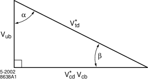
Figure 1: The right unitarity triangle.

In any case, we inquire here what dynamical mechanism might be responsible for such a situation. There is a very natural answer, namely that the ordinary down-quarks $d_{i}=(d,s,b)$ mix with heavy down-quarks $D_{i}=(D,S,B)$ which are electroweak singlets and have large intrinsic mass terms $M_{i}$. There is no mass mixing in the up sector simply because the corresponding heavy up degrees of freedom do not exist.

Such heavy down states are not altogether unwelcome. In GUT extensions which go by way of $E(6)$, the fundamental $\underline{27}$ representation contains just such a multiplet. The $SU(5)$ decomposition of this $E(6)$ $\underline{27}$ is

$$27=(\overline{10}+5)+(5+\overline{5})+(1+1)\ .$$ (18)

We notice that if this is the scenario, then there will also be heavy leptons $L_{i}=(E,M,T)$ which are vector electroweak doublets, i.e. both the left-handed and right-handed components of the $L_{i}$ couple to the $W$’s. We shall here accept that this is the case, because even without $E(6)$ one would have a problem with anomaly cancellation if only the heavy down-quarks $D_{i}$ were introduced. Adding in the $L_{i}$ clearly solves the anomaly problem.

The mass mixing term for the down-quarks, as shown in Fig. 2 (consistent with $SU(2)\times U(1)$ electroweak symmetry), now can be written down:

$${\cal L}^{\prime}_{\mu}=\sum_{ij}\overline{D}_{iL}\,\mu_{ij}\,d_{jR}+{\rm h.c.}$$ (19)

with, perhaps, $\mu_{ij}$ having the form of Eq. (17). In addition we must introduce intrinsic mass terms (taken to be real) for the heavy down-quarks (also consistent with electroweak gauge symmetry)

$${\cal L}^{\prime}_{M}=\sum_{i}M_{i}\overline{D}_{iL}D_{iR}+{\rm h.c.}$$ (20)

This much does not by itself give mass to the light down-quarks, because their left-handed components are as yet not coupled. This is remedied by assuming that the Higgs bosons couple the heavy right-handed down-quarks to the left-handed ordinary quarks.

$${\cal L}^{\prime}_{H}=\sum_{i}\overline{q}_{iL}\Phi H_{i}D_{iR}+{\rm h.c.}$$ (21)

where

$$q_{i}\equiv{u_{i}\choose d_{i}}\qquad\Phi=(v+\phi)+i\mbox{\boldmath$\tau$\unboldmath}\cdot{\bf w}$$ (22)

and

$$H_{i}\equiv\left(\begin{array}[]{cc}0&0\\ 0&H_{i}\end{array}\right)\ .$$ (23)

Then the mass matrix of the light quarks is obtained by diagonalization, essentially second-order perturbation theory:

$$m_{ij}\cong(H_{i}v)\ \frac{1}{M_{i}}\,\mu_{ij}\ .$$ (24)

with our convention that

$${\cal L}^{(\rm effective)}_{m}=\overline{d}_{iL}\,m_{ij}\,d_{jR}+{\rm h.c.}$$ (25)

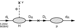
Figure 2: Mixing mechanism for the down-quark masses.

Note that we take care to omit the usual Higgs coupling between the right-handed ordinary down-quarks $d_{i}$ and the ordinary left-handed quarks. This assumption is robust in the sense that, if the terms in the mass matrix which mix $d$ and $D$ are neglected, the full Lagrangian as written possesses enough symmetry that such Yukawa terms will not be generated by radiative corrections. This conclusion follows immediately from the fact that in that limit the right-handed $d$’s decouple completely from the Higgs sector. In other words, the number of $d_{R}$’s of each generation is, in the absence of the mass-mixing term, Eq. (19), conserved. Inclusion of the kinetic energy terms and gauge couplings still leaves the Lagrangian invariant under independent phase transformations of the $d_{R}$’s. Therefore for small $\mu$ and $m$, as we shall see, the $\mu$ dependent terms are finite and calculable.

We will need to include in the Lagrangian the usual Higgs couplings of the right-handed up-quarks $u_{i}=(u,c,t)$ to their left-handed counterparts. However recall again that these couplings are assumed to be flavor diagonal. Just to set the notation, the Lagrangian for these terms is

$${\cal L}^{\prime}_{h}=\sum_{i}\overline{q}_{iL}\,\Phi\,h_{i}\,u_{iR}\qquad h_{i}\equiv\left(\begin{array}[]{cc}h_{i}&0\\ 0&0\end{array}\right)\ .$$ (26)

We should also include the gauge boson terms as well. However, for almost all purposes in this paper, we can neglect their presence, remembering that in the limit of vanishing gauge couplings the longitudinal $W$ and $Z$ become the massless Goldstone modes of the Higgs sector.

It is important to estimate as well as possible the magnitudes of the new parameters. The new Yukawa couplings $H_{i}$ may be rather large, of order of the top quark coupling $h_{t}$ or larger, and as we shall see this case appears to be an interesting one. The magnitudes of the masses of the new down-quarks and leptons will be constrained from below by the precision electroweak data and perhaps from above by the properties of the Higgs-potential radiative corrections. The nominal values are in the 1–10 TeV regime. The constraints on the parameters will be considered in more detail in the next section.

However before turning to that, we are ready to diagonalize the mass matrix of the quarks. We write the 6$\times$6 undiagonalized mass matrix ${\cal M}^{\prime}$ in block form as

$${\cal M}^{\prime}=\left(\begin{array}[]{cc}0&Hv\\ \mu&M\end{array}\right)\ ,$$ (27)

where the indices 1,2,3 label the ordinary light quarks $d_{i}$ and 4,5,6 the new heavy quarks $D_{i}$. This matrix is not hermitian, so we diagonalize its square ${\cal M}^{\prime}{\cal M}^{\prime\dagger}$, because it is the left-handed mixing which we need to see explicitly in the CKM phenomenology. Note that $H$ and $M$ are 3$\times$3 diagonal matrices, so that we may write

$${\cal M}^{\prime}{\cal M}^{\prime\dagger}=\left(\begin{array}[]{cc}H^{2}v^{2}&HvM\\ HvM&\mu\mu^{\dagger}+M^{2}\end{array}\right)={\cal V}{\cal M}^{2}{\cal V}^{\dagger}\ ,$$ (28)

where ${\cal M}$ by definition is diagonal, and we are to find ${\cal V}$. A first prediagonalization is immediate, if one ignores the (small) terms $\mu$ associated with the flavor and CP violation. In this approximation, the diagonalizing matrix ${\cal V}$ is 3$\times$3 block diagonal

$${\cal V}=\left(\begin{array}[]{cc}c&s\\ -s&c\end{array}\right)$$ (29)

where

$$s\cong\frac{Hv}{M}\equiv\left(\begin{array}[]{ccc}\sin\theta_{1}&0&0\\ 0&\sin\theta_{2}&0\\ 0&0&\sin\theta_{3}\end{array}\right)$$ (30)

and

$$c^{2}+s^{2}=1\ .$$ (31)

We will find in the next section that these mixing angles cannot be large. The reason is simple; the electroweak-doublet nature of the left-handed quarks is diluted by the mixing, and the $W$ and $Z$ do not couple to the singlet portion with the same strength as to the doublet portion. Therefore there are renormalizations of the strengths of the diagonal couplings of $W$ and $Z$ to quark pairs, and the precision electroweak data restricts these renormalizations to be no larger than the 1% level. Since the depletions are proportional to the square of the mixing angles, this limits the $s_{i}$ to no more than the 10% level.

Now let us examine in more detail the residual nondiagonal terms. Thus far we have

$${\cal V}^{\dagger}({\cal M}^{\prime}{\cal M}^{\prime\dagger}){\cal V} = \left(\begin{array}[]{cc}0&0\\ 0&M^{2}+H^{2}v^{2}\end{array}\right)+{\cal V}^{\dagger}\left(\begin{array}[]{cc}0&0\\ 0&\mu\mu^{\dagger}\end{array}\right)\,{\cal V}$$ (36)

$$= \left(\begin{array}[]{cc}s\mu\mu^{\dagger}s&-s\mu\mu^{\dagger}c\\ \ \ -c\mu\mu^{\dagger}s&c\mu\mu^{\dagger}c+M^{2}+H^{2}v^{2}\end{array}\right)\ .$$ (39)

We see that, as expected, the mass matrix of the light quarks to this order is

$$mm^{\dagger}\cong(s\mu)(s\mu)^{\dagger}$$ (40)

with

$$m=s\mu=\frac{Hv}{M}\ \mu$$ (41)

consistent with Eq. (24). Without going further we see from Eq. (39) that if the $s_{i}$ are flavor universal, then diagonalization with the CKM matrix suffices to diagonalize to all orders the full mass matrix. However, this is not true in general. More generally, the next-order correction to the light quark mass matrix has the form

$$\Delta(mm^{\dagger}) = (s\mu\mu^{\dagger}c)\ \frac{1}{M^{2}+H^{2}v^{2}}\ (c\mu\mu^{\dagger}s)=(s\mu\mu^{\dagger}s)\ \frac{c^{2}}{s^{2}(M^{2}+H^{2}v^{2})}\ (s\mu\mu^{\dagger}s)$$ (42)

$$= (s\mu\mu^{\dagger}s)\ \left[\frac{1}{H^{2}v^{2}}-\frac{1}{(M^{2}+H^{2}v^{2})}\right]\ (s\mu\mu^{\dagger}s)\ .$$

In any case, the flavor- and CP-violation effects are concentrated in a semisoft mass term. This in turn leads to only small, finite, calculable corrections to the Yukawa couplings and heavy-quark mass terms. As will be demonstrated in more detail in the next section, flavor violation in this model becomes an “infrared” phenomenon only. Flavor nonuniversality, i.e. diagonal flavor-conserving couplings depending upon the generation, will however persist more than does the flavor violation. But these will be small if the $H_{i}$ and $M_{i}$ are flavor universal. (Of course the up-quark couplings $h_{i}$ cannot be flavor-universal, and that nonuniversality alone suffices to create corrections in all the other couplings via radiative effects.)

In the lepton sector, things are slightly different. The left-handed charged leptons, $\ell_{L}\equiv(e,\mu,\tau)$ mix with the heavy leptons, $L^{-}\equiv(E,^{-}M,^{-}T^{-})$ via a semi-soft mass term $\widetilde{\mu}$ like the d-quarks while the right-handed ones $\ell_{R}$ couple to $L^{-}_{L}$ via the Higgs Yukawa couplings yielding a 6$\times$6 mass matrix of the form

$${\cal M}_{\ell}=\left(\begin{array}[]{cc}0&\widetilde{H}v\\ \widetilde{\mu}&\widetilde{{\cal M}}\end{array}\right)\ .$$ (45)

Just as for the quarks, there is again no Yukawa coupling term which would couple the ordinary light leptons $\ell_{L}$ to the $\ell_{R}$. This time a nonvanishing additive quantum number assigned to the ordinary left-handed lepton electroweak doublet $(\ell,\nu_{\ell})_{L}$ and to nothing else suffices, in the absence of the flavor-changing mixings proportional to $\mu$, to forbid the presence of this Yukawa coupling. Alternatively, the left-handed lepton doublet might be assigned a multiplicative “parity” quantum number -1; with all other multiplets having positive parity. Note that this assignment survives the extension to the GUT $SU(5)$ level.

In the neutrino sector, the mixing of $\nu^{i}_{L}$ with the $E^{0}_{L}$ leaves the neutrinos massless. But the mixing of $\nu_{L}$ with the $SU(5)$-singlet fermions present in the $E(6)$ extension will give rise to neutrino masses and mixings. In principle we need not introduce these extra degrees of freedom $(N,N^{\prime})$ at all. But there is ample motivation for doing so, and we return in the next section to a discussion of the implications.

The upshot of all this is that there is a 6$\times$6 unitary matrix diagonalizing the charged lepton mass matrix with a structure very similar to the one for down-quarks:

$$\widetilde{U}_{6}=\left(\begin{array}[]{cc}\widetilde{U}_{3}&0\\ 0&1\\ \end{array}\right)\left(\begin{array}[]{cc}\widetilde{c}&\widetilde{s}\\ -\widetilde{s}&\widetilde{c}\end{array}\right)$$ (46)

with $\widetilde{s}_{i}\approx\widetilde{H}_{i}v/\widetilde{M}_{i}$ etc. The feature of nonuniversality of diagonal couplings will persist, and the phenomenology differs slightly due to the fact that the heavy leptons are vector-like electroweak doublets, not singlets.

Before going on, we summarize how the tree level couplings to $W$ and $Z$ are modified by the mixing effects. For the $W$, there will be the usual CKM structure, but modified by the effects of the mixing to the heavy down-quarks expressed by ${\cal V}$. Thus

$$G_{F}\overline{u}_{iL}\gamma^{\mu}(V_{CKM})_{ij}d_{jL}\Rightarrow G_{F}\,\left\{\overline{u}_{iL}\gamma^{\mu}(V_{CKM})_{ij}c_{j}d_{jL}\ +\overline{u}_{iL}\gamma^{\mu}(V_{CKM})_{ij}s_{j}D_{jL}\right\}.$$ (47)

In the same way the leptonic coupling strengths to the $W$ are modified:

$$G_{F}\overline{\nu}_{iL}\gamma^{\mu}\ell_{iL}\Rightarrow G_{F}\left\{\overline{\nu}_{iL}\gamma^{\mu}(V_{MNS})_{ij}\widetilde{c}_{j}\ell_{jL}+\overline{\nu}_{iL}\gamma^{\mu}(V_{MNS}){{}_{ij}}\widetilde{s}_{j}L^{-}_{jL}-\overline{L}^{0}_{iL}\gamma^{\mu}\widetilde{s}_{i}\ell_{iL}\right\}$$ (48)

where the leptonic mixings $\widetilde{s}_{i},\widetilde{c}_{i}$, are introduced in analogy to the quark mixings $s_{i},c_{i}$ (Eq. (29)), and in general are different. The leptonic mixing matrix $V_{MNS}$ (named after Maki, Nakagawa and Sakata [19]) is the analog of the CKM matrix in the quark sector. It is given by

$$V_{MNS}=U^{\dagger}_{\nu}\ \widetilde{U}_{3}\ ,$$ (49)

where $U_{\nu}$ is the matrix which diagonalizes the neutrino mass matrix. In addition, there are new right-handed leptonic charged currents given by:

$${\cal L}^{\prime}_{L}=G_{F}\overline{L}^{0}_{iR}\ \gamma^{\mu}(-\widetilde{s}_{i})\ell_{iR}\ .$$ (50)

The couplings of light down-quarks to the $Z$ are affected. Starting from the usual structure

$${\cal L}_{NC}\propto T_{3}-\sin^{2}\theta_{W}Q\ ,$$ (51)

only the $T_{3}$ portion will be affected by all this mixing; charge conservation protects the rest. The effect of the heavy-light mixing is, for the quarks,

$$(\overline{u}_{iL}\gamma^{\mu}u_{iL}-\overline{d}_{iL}\gamma^{\mu}d_{iL})Z^{\mu}\Rightarrow(\overline{u}_{iL}\gamma^{\mu}u_{iL}-c^{2}_{i}\overline{d}_{iL}\gamma^{\mu}d_{iL})Z_{\mu}-c_{i}s_{i}\overline{d}_{iL}\gamma^{\mu}D_{iL}Z_{\mu}+h.c.$$ (52)

For the leptons,

$$(\overline{\nu}_{i}\gamma^{\mu}\nu_{i}-\overline{\ell}_{iL}\gamma^{\mu}\ell_{iL})Z^{\mu}\Rightarrow(\overline{\nu}_{i}\gamma^{\mu}\nu_{i}-\overline{\ell}_{iL}\gamma^{\mu}\ell_{iL}-\widetilde{s}_{i}^{2}\overline{\ell}_{iR}\gamma^{\mu}\ell_{iR}+\widetilde{s}_{i}\widetilde{c}_{i}\overline{\ell}_{iR}\gamma^{\mu}L_{iR})Z^{\mu}\ .$$ (53)

The phenomenological implications of these and other modifications will be taken up in the next section.

3.1 Neutrino Masses

Neutrino mixing with $E^{0}$ gives rise to a mass matrix (for each flavor) of the form:

$$\left(\begin{array}[]{ccc}0&m\\ 0&M\end{array}\right)\ .$$ (56)

This has one zero eigenvalue and so the neutrinos remain massless. When one of the two gauge singlets, $N$, is included, the mass matrix becomes:

$$\left(\begin{array}[]{ccc}0&m&m^{\prime}\\ 0&M&0\\ m^{\prime}&0&M^{\prime}\end{array}\right)\ .$$ (60)

The neutrino mass eigenvalue is now given by the usual see-saw formula:

$$m_{\nu}\sim m^{\prime 2}/M^{\prime}\ .$$ (61)

If the Dirac masses $m^{\prime}$ are taken to be of the order of the top-quark mass, then the mass scale $M^{\prime}$ lies in the range of $10^{14}$ GeV in order to accommodate the typical mass scales required in the atmospheric and solar neutrino oscillations. This is lower than the unification scale, and might represent an oasis. The other singlet $N^{\prime}$ might be at the unification scale. To make some ansatz about the flavor structure of the lepton and neutrino mass matrices, which would lead to a desirable form for the MNS matrix, is beyond the scope of this paper and we leave it to another occasion.

4 Phenomenological Implications

4.1 Decay Widths

The masses of the new heavy quarks and leptons are free parameters in this model. As we shall soon see, unless the Higgs couplings $H_{i}$ are small, there are difficulties with precision electroweak data if these masses are low. The experimental constraints will, as discussed below, generically lead to bounds on the mixing angles $s_{i}$ and $\widetilde{s}_{i}$, as defined in Eq. (30):

$$|s_{i}|=\left|\frac{H_{i}v}{M_{i}}\right|\buildrel<\over{{}_{\sim}}0.1\ .$$ (62)

If the masses are large in comparison with the gauge boson and even Higgs masses, the decay phenomenology of the new heavy fermions is quite straightforward: they will decay predominantly into the ordinary quark or lepton of the same generation together with either a Higgs or a (longitudinal) gauge boson. For example, for the third generation $B$ we have the decay modes

$$B \rightarrow b+h$$ (63)

$$B \rightarrow b+Z^{0}$$ (64)

$$B \rightarrow t+W^{-}$$ (65)

with

$$\Gamma(B\rightarrow bh)=\Gamma(B\rightarrow bZ^{0})=\frac{1}{2}\,\Gamma(B\rightarrow tW^{-})\ .$$ (66)

The total decay width is, in the limit of negligible final-state masses,

$$\Gamma(B\rightarrow{\rm all})\cong\frac{H^{2}_{B}}{4\pi}\ M_{B}\ .$$ (67)

The main usefulness of this formula is to provide a practical upper bound on the magnitude of the Higgs couplings $H_{i}$; the theory makes little sense if the width of the parent fermion is larger than its mass. In particular this constraint implies

$$|H_{i}|\leq 4$$ (68)

or

$$\frac{H^{2}_{i}}{4\pi}\buildrel<\over{{}_{\sim}}1\ .$$ (69)

The decay phenomenology for heavy leptons is essentially identical; the decay modes for the third generation $T$ are given by:

$$T^{-}\longrightarrow\tau^{-}+Z^{0}$$

$$T^{-}\longrightarrow\tau^{-}+h^{0}$$ (70)

$$T^{0}\longrightarrow\tau^{-}+W^{+}$$

and the widths satisfy

$$\Gamma(T^{-}\rightarrow\tau^{-}h^{0})=\Gamma(T^{-}\rightarrow\tau^{-}Z^{0})=\frac{1}{2}\Gamma(T^{0}\rightarrow\tau^{-}W^{+})\ .$$ (71)

The total widths are given by:

$$\Gamma_{tot}(T^{-})=\Gamma_{tot}(T^{\circ})=\frac{\widetilde{H_{T}}^{2}\widetilde{M_{T}}}{8\pi}$$ (72)

and thus $\widetilde{H}_{i}$ satisfy bounds similar to $H_{i}$.

In the above scenario, the search strategies for these particles are in principle straightforward. The main issue is attaining sufficient energy to produce them.

On the other hand, if some of the new Yukawa couplings $H_{i}$ are small, then the associated masses can be small as well. However, we shall consider it unreasonable that all the new quarks have Yukawa couplings to the Higgs sector much smaller than the coupling of the top quark to the Higgs. In particular we hereafter assume that the third generation down-quark $B$ has a Yukawa coupling at least as large as that of the top quark:

$$H_{B}\geq h_{t}\cong 0.70\ .$$ (73)

We shall see later that this innocent hypothesis leads to interesting consequences.

Within this scenario there are still major choices to make. One extreme is to assume flavor symmetry for the new heavy down-quark multiplet:

$$M_{B}\approx M_{S}\approx M_{D}$$

$$H_{B}\approx H_{S}\approx H_{D}.$$

The other extreme is to assume a mass and coupling constant hierarchy as found everywhere else in the spectrum of fermion degrees of freedom:

$$M_{B}\gg M_{S}\gg M_{D}$$

$$H_{B}\gg H_{S}\gg H_{D}\ .$$ (74)

While many variants can be entertained, in what follows we restrict our attention to these two extremes. In particular, in the hierarchial choice, we find no reason why the first and second generation heavy quarks and leptons cannot be as light as given by the present direct experimental limit on their production, about 130 GeV [20]. If such masses do approach the direct experimental limits for production of heavy quarks and leptons, the phenomenology may differ significantly. However, one must keep in mind that a large violation of universality of the new parameters $H_{i}$ and $M_{i}$ may be constrained by precision electroweak data. These are discussed in the following subsections.

4.2 Tree-Level Mixings

In the previous section we have exhibited the effective Lagrangian obtained by diagonalization of the mass matrix of the light quarks. In addition to leaving behind the CKM mixing of the quark couplings to the $W$ bosons, we have seen there are nonuniversal diagonal couplings to the $Z$ boson, which lead to deviations of the values of electroweak parameters from the standard model values. The percentage deviations will be proportional to the squares of the mixing angles $s_{i}$ introduced in Eq. (30). For example, the branching fraction $R_{b}$ for $Z$ decay into $\overline{b}b$ is modified as follows

$$R_{b}\rightarrow R_{b}^{SM}\left[1-\frac{2s^{2}_{3}\left(1-\frac{2}{3}\sin^{2}\theta_{W}\right)}{\left(1-\frac{4}{3}\sin^{2}\theta_{W}+\frac{8}{9}\sin^{4}\theta_{W}\right)}\right]$$ (75)

with similar expressions, of course, for decays into $\overline{s}s$ or $\overline{d}d$. Likewise the forward-backward asymmetry $A_{FB}$ in $Z$ decays to $\overline{b}b$ is modified as follows:

$$(A_{FB})_{b}\rightarrow(A_{FB})_{b}^{SM}\,\left[1-\frac{\frac{16}{9}\,s^{2}_{3}\sin^{4}\theta_{W}\left(1-\frac{2}{3}\sin^{2}\theta_{W}\right)}{\left(1-\frac{2}{3}\sin^{2}\theta_{W})^{4}-(\frac{2}{3}\sin^{2}\theta_{W}\right)^{4}}\right]\ .$$ (76)

Modifications to the diagonal couplings of the $Z$ to leptons is also of significance. The most sensitive constraint comes from measurements of the polarization asymmetry $A_{LR}$. The correction modifies $A_{LR}$ as:

$$A_{LR}=\frac{2(1-4\sin^{2}\theta_{W})+8\sin^{2}\theta_{W}\widetilde{s}^{2}_{1}}{1+(1-4\sin^{2}\theta_{W})^{2}-8\sin^{2}\theta_{W}\widetilde{s}^{2}_{1}}\ .$$ (77)

However, competitive tests also come from the measurement of the axial couplings $g_{A}$ of the $Z$ to lepton pairs. The mixing correction decreases $g_{A}$

$$g_{A_{i}}=(g_{R}-g_{L})_{i}=(T_{3}\widetilde{s}^{2}_{i}-\sin^{2}\theta_{W}Q)-(T_{3}-\sin^{2}\theta_{W}Q)=\frac{1}{2}\,(1-\widetilde{s}^{2}_{i})\ .$$ (78)

In all these cases the current data are consistent with the standard model. From LEP and SLC data, deviations from the standard model are bounded [21] and yield bounds in turn on $s_{3}$ and $\widetilde{s}_{1}$ of about 0.1 and 0.05 respectively. Similar bounds can be deduced for $s_{1}$, $\widetilde{s}_{2}$, and $\widetilde{s}_{3}$. We expect similar bounds on the other mixing angles. The bound on $s_{3}$ comes from $R_{b}$. Should the current discrepancy in $A_{FB}$ of $-0.0046\pm 0.0017$ turn out to be real, we cannot account for it (an $s_{3}$ of 0.1 allows a maximum deviation of $-$0.001).

4.3 Mixings at One-Loop

4.3.1 Flavor Mixing

The modified charged currents in Eq. (38) and (39) have a very special form. In particular, even though the effective 3$\times$3 CKM (or MNS) matrix is not unitary, it has partial orthogonality i.e.

$$\sum_{i=u,c,t}\left(V_{CKM}\right)_{bi}^{*}\left(V_{CKM}\right)_{is}=c_{3}c_{2}\sum_{i}U_{3i}^{*}U_{i2}=0$$ (79)

and similarly:

$$\sum_{i=\nu_{1},\nu_{2},\nu_{3}}\left(V_{MNS}\right)_{\mu i}^{*}\left(V_{MNS}\right)_{ie}=0\ .$$ (80)

However, this is not true in the up-quark sector:

$$\sum_{i=d,s,b}\left(V_{CKM}\right)_{ci}^{*}\left(V_{CKM}\right)_{iu}\neq 0\ .$$ (81)

This means that there are no new one-loop flavor changing effects in the down-quark sector or the lepton sector. Hence, there are no new contributions beyond the standard model in: (i) $\delta m_{K}$, (ii) $\epsilon$, (iii) $\epsilon^{\prime}/\epsilon$, (iv) $\delta m_{B}$, (v) b $\rightarrow s\gamma$ or $b\rightarrow d\gamma$, (vi) CP violating effects in the b-quark sector, (vii) $\mu\rightarrow e\gamma$, (viii) $K_{L}\rightarrow\mu e$ etc. This is a strong prediction of this set of ideas.

There is a potential new contribution to $D^{0}-\overline{D^{0}}$ neutral charm meson mixing due to the heavy quarks in the box diagram. Assuming for simplicity that the heavy $S$ quark dominates, the new contribution to $\delta m_{D}$ is given by [22]

$$\delta m_{D}=\frac{G_{F}^{2}}{6\pi^{2}}\ f^{2}_{D}\ B_{D}\ m_{D}\ m^{2}_{W}\ s_{2}^{4}\left(V^{*}_{cs}V_{su}\right)^{2}\ f(x_{S})\ .$$ (82)

For large $M_{S},f(x_{S})\approx M_{S}^{2}/4m_{W}^{2}$ and $\delta m_{D}$ becomes:

$$\delta m_{D} = \frac{G_{F}^{2}}{24\pi^{2}}\ f^{2}_{D}\ B_{D}\ m_{D}\ M^{2}_{S}\ s_{2}^{4}\ \theta^{2}_{c}$$

$$= (2\times 10^{-9}s^{4}_{2})\,GeV(M_{S}/1\ TeV)^{2}\ .$$

If the heavy $S$ quark is replaced by $D$, a similar bound is obtained. If $S$ is replaced by $B$, the contribution is much smaller.

The current bound on $\delta m_{D}$ is $5\times 10^{-14}$ GeV and demands $s_{2}<0.07$. This remains a potential significant contribution to $\delta m_{D}$.

4.3.2 S, T and U Parameters

A convenient parametrization which describes new physics contributions to electroweak radiative corrections is given by the $S,T,U$ formalism of Peskin and Takeuchi [23]. These parameters are defined such that deviations from zero would signal the existence of new physics (an alternate set of parameters, $\epsilon_{i}$ also exist which do not require a reference point for the standard model [24]).

The contributions from the extra fermions introduced here are rather small as shown in Ref. [25]. At a mass scale of $O(TeV)$ the contributions to $S,T$ and $U$ are no more than a few times $10^{-3}$ and well within the current bounds, as long as the heavy lepton doublets are nearly degenerate.

4.3.3 Anomalous Magnetic Moment of the Muon

The extraordinary precision of the $g-2$ measurements suggests that significant constraints on our mixing and mass parameters might exist. With this in mind we consider the contribution of the heavy leptons $M^{-}$ and $M^{0}$ to $a_{\mu}$. There are two Feynman diagrams as given in Fig. 3. We let $M_{M}^{-}\approx M_{M}^{0}\approx M_{M}$ each be about a TeV. Then the total contribution to $a_{\mu}=(g-2)_{\mu}$ is given by [26, 27].

$$a_{\mu}=\frac{G_{F}m^{2}_{\mu}}{4\sqrt{2}\pi^{2}}(\widetilde{s}_{2})^{2}\{F+H\}$$ (84)

where $F$ and $H$ are slowly varying functions of $(M_{M}/M_{Z})^{2}$ and $(M_{M}/M_{W})^{2}$ respectively [26, 27]. For the value $M_{M}\sim 1\ TeV$, the combination $\{F+H\}\approx+1/3$ and $a_{\mu}$ is given by:

$$a_{\mu}\sim(\widetilde{s}_{2})^{2}\ 74\times 10^{-11}$$ (85)

and for $\widetilde{s}_{2}\sim$ 0.1, this contributes to $a_{\mu}$ something less than $10^{-11}$.

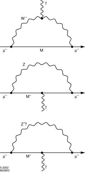
Figure 3: Feynman graphs for the ($g-2$) correction.

If the extra $Z^{\prime}$ contained in $E(6)$ is relatively light, say of order $1\ TeV$; then there is a potentially large contribution to the $a_{\mu}$ from the Feynman diagram in Fig. 3 where both $M_{M}$ and $Z^{\prime}$ appear in the loop. The dominant contribution to $a_{\mu}$ from this graph is given by [26, 27].

$$a_{\mu}=\frac{\alpha^{\prime}}{2\pi}\frac{m_{\mu}}{M_{z}^{\prime}}^{2}(\widetilde{s}_{2})^{2}\widetilde{G}(\frac{M_{M}}{m_{\mu}})X$$ (86)

where $X$ is given by:

$$X=\left[-(x^{\mu}_{L}-x^{M}_{L})(x^{\mu}_{R}-x_{R}^{M})\right],$$ (87)

$\widetilde{G}$ is a slowly varying function of $(M_{M}/M_{Z}^{\prime})^{2}$, and $(M_{M}/m_{\mu})$ is the enhancement due to chirality violation. For $(M_{M}/M_{Z}^{\prime})\sim 1$, the function $\widetilde{G}$ is close to 1/2. The value of $X$ depends on the details of how the symmetry is broken from $E(6)$ and can be as large as $+~{}18$ as shown in Ref. [28]. Then, for $\alpha^{\prime}\sim\alpha$,

$$a_{\mu}(Z^{\prime})\sim(\widetilde{s}_{2})^{2}\ 504\times 10^{-11}\ .$$ (88)

If $\widetilde{s}_{2}$ is about 0.1, then this contribution to $a_{\mu}$ can be no more than $5\times 10^{-11}$ and is not important.

We conclude that the sensitivity of the $g-2$ measurements appears to be somewhat milder than the other precision electroweak measurements we have considered.

4.4 One-loop Modification of the Higgs Effective Potential

The new one-loop contributions to the Higgs potential are of considerable interest. Recall that the renormalized standard-model effective potential can be written, up to a quadratic polynomial in $\phi^{2}$, as

$$V \simeq \frac{\lambda}{4}(\phi^{2}-v^{2})^{2}$$

$$+\ \frac{\lambda^{2}(3\phi^{2}-v^{2})^{2}}{64\pi^{2}}\,\ell n\,\frac{(3\phi^{2}-v^{2})}{2v^{2}}$$

$$+\ \frac{3\lambda^{2}}{64\pi^{2}}\ (\phi^{2}-v^{2})^{2}\,\ell n\,\frac{(\phi^{2}-v^{2})}{v^{2}}$$

$$-\ \frac{12m^{4}_{t}}{64\pi^{2}}\ \frac{\phi^{4}}{v^{4}}\,\ell n\,\frac{\phi^{2}}{v^{2}}$$

$$+\ \frac{3}{64\pi^{2}}\,(2m^{4}_{W}+m^{4}_{Z})\,\frac{\phi^{4}}{v^{4}}\,\ell n\,\frac{\phi^{2}}{v^{2}}\ .$$

where the radiative terms are renormalized such that only the logarithmic terms are kept and that at $\phi^{2}=v^{2}$ they vanish. Note that in this scheme there will be residual finite radiative corrections to the vacuum condensate strength $v^{2}$.

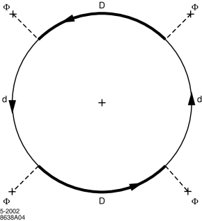
Figure 4: Heavy down-quark contribution to the effective potential.

The new contribution after renormalization has a very interesting structure due to the fact that the new fermion loop has equal numbers of heavy-quark segments and light-quark segments (Fig. 4):

$$\delta V=-\frac{12}{64\pi^{2}}\sum^{3}_{i=1}\,\left(M^{2}_{i}+H^{2}_{i}\phi^{2}\right)^{2}\,\ell n\,\frac{M^{2}_{i}+H^{2}_{i}\phi^{2}}{M^{2}_{i}+H^{2}_{i}v^{2}}\ .$$ (90)

The important feature is that at scales below the heavy-fermion mass scale $M$, there is a new (finite!) quadratic mass term for the Higgs lagrangian, with negative coefficient.

$$\delta V \cong -\frac{12}{64\pi^{2}}\sum^{3}_{i=1}\,H^{2}_{i}(M^{2}_{i}+H^{2}_{i}v^{2})^{2}(\phi^{2}-v^{2})/M_{i}^{2}$$ (91)

$$\cong -\frac{12}{64\pi^{2}}\sum^{3}_{i=1}H^{2}_{i}M^{2}_{i}(\phi^{2}-v^{2}).$$

This means that the spontaneous symmetry breaking can be induced radiatively via these new heavy fermions.

One may question whether this conclusion is significant, since it is an argument on the structure of the renormalization constant $v^{2}$. One might argue that a quadratic polynomial in $\phi^{2}$, with coefficients dependent on $H_{i}$ and $M$, should be appended to Eq. (90) such that, in the limit $M_{i}\rightarrow\infty$, $\delta V$ vanishes. This would be in accordance with Appelquist-Carrazone [29] behavior—although the arguments of Appelquist and Carrazone do not strictly apply to this case. Evidently such a counterterm will eliminate the quadratic term of interest in Eq. (91). But it seems equally reasonable to take Eq. (90) to be the basic structure of the radiative correction, with the “Appelquist-Carrazone” cancellation regarded as unnatural “fine tuning”. In this case it is the limit $M_{i}\rightarrow 0$ for which $\delta v$ vanishes. Without better control of the quadratic-divergence issue, the situation appears to us to be ambiguous. We shall assume in what follows that the form of Eq. (90) faithfully represents the true radiative correction.

Either this radiative term, Eq. (90), is the predominant contribution to the top of the “Mexican hat”, or else it is a correction. But we shall consider it to be “unnatural” to suppose that this finite piece is cancelled off to high accuracy by something else. Therefore one may expect that its magnitude is limited by the known size of the Mexican-hat term. This gives the rough bound

$$\frac{12}{64\pi^{2}}\sum^{3}_{i=1}\,H^{2}_{i}M^{2}_{i}\buildrel<\over{{}_{\sim}}(1\ TeV)^{2}$$ (92)

leading to

$$7\ TeV\buildrel>\over{{}_{\sim}}\sqrt{\sum^{3}_{i=1}H^{2}_{i}M^{2}_{i}}\geq H_{B}M_{B}\geq h_{t}M_{B}=0.7\,M_{B}$$ (93)

where we have used our assumed lower bound on $H_{B}$ from Section 4.1.

The bottom line is that, together with the lower bound on $M_{B}$ coming from the precision electroweak measurements

$$|s_{3}|=\left|\frac{H_{B}v}{M_{B}}\right|\buildrel<\over{{}_{\sim}}0.1\ ,$$ (94)

leading to

$$M_{B}\geq 10\ H_{B}v\geq 10\ h_{t}v=10\ m_{t}=1.7\ TeV\ ,$$ (95)

we may infer

$$1.7\ TeV\buildrel<\over{{}_{\sim}}M_{B}\buildrel<\over{{}_{\sim}}10\ TeV\ .$$ (96)

We may also infer that the remaining down-quarks are no heavier. If the well-known symmetry relation connecting $m_{b}$ and $m_{\tau}$

$$\frac{m_{\tau}}{m_{b}}\approx\left[\frac{\alpha_{s}(m^{2}_{\rm GUT})}{\alpha_{s}(m^{2}_{b})}\right]^{0.5}\approx 0.3$$ (97)

can be applied to this heavy sector, then the generalization of Eq. (96) to the third-generation leptons $T$ would read

$$0.8\ GeV\buildrel<\over{{}_{\sim}}M_{T}\buildrel<\over{{}_{\sim}}5\ TeV\ ,$$ (98)

with the remaining leptons (other than possibly the gauge singlets $N_{i},N^{\prime}_{i}$) no heavier.

5 Running Coupling Constants

5.1 The Fermion-Higgs Sector

The presence of new heavy fermions, with assumed masses which are not too heavy, implies that the usual considerations of the scale-dependence of the dynamics needs to be modified. In the standard model, the top-quark Yukawa coupling is almost large enough for it to attain strong coupling at an energy scale below the GUT scale. Also, the Higgs-boson quartic coupling will become strong below the GUT scale unless its mass lies in the relatively narrow window of 140–180 GeV.

It is of course a very central question whether there exists “oases” in the desert, i.e. energy scales small compared to the GUT scale, where some subset of interactions become strong. Thus far, the introduction of these new fermions has not demanded any new oasis. However, as we shall see, one or more oases can occur because of the extra loading of the renormalization-group equations from the new degrees of freedom.

We first review the standard-model situation, working to one-loop order, and neglecting small contributions, e.g. from gauge degrees of freedom, whenever possible. The important quantities are the top quark coupling $h_{t}\equiv h$, and the Higgs quartic self-coupling $\lambda$. Ignoring all gauge couplings except the important QCD correction, one has

$$\frac{dh^{2}}{dt}=9h^{4}-8g^{2}h^{2}$$ (99)

and

$$\frac{d\lambda}{dt}=12\,(\lambda^{2}+\lambda h^{2}-h^{4})$$ (100)

where our notation is

$$t = \frac{1}{16\pi^{2}}\,\ell n\,\frac{\mu^{2}}{\Lambda^{2}_{QCD}}$$

$$\frac{1}{g^{2}(t)} = \left(11-\frac{2}{3}\,n_{f}\right)t\simeq 7t$$ (101)

$$\lambda(0.1) = \lambda_{EW}=\frac{m^{2}_{H}}{2v^{2}}\ ,\quad v\approx 250\ GeV\,.$$

This gives for the scale parameter $t$ the values 0, 0.1, and 0.5 at the QCD, electroweak, and GUT scales respectively.

In our model, these equations become modified at scales large compared to the scale $M$ of the heavy quark masses. The modifications are as follows:

$$\frac{dh^{2}}{dt} = 9h^{4}+6h^{2}\sum^{3}_{j=1}\,H^{2}_{j}-8g^{2}h^{2}$$

$$\frac{dH^{2}_{i}}{dt} = 3H^{4}_{i}+6H^{2}_{i}\left(h^{2}+\sum^{3}_{j=1}H^{2}_{j}\right)-8g^{2}H^{2}_{i}$$ (102)

$$\frac{d\lambda}{dt} = 12\lambda^{2}+12\lambda\,\left(h^{2}+\sum^{3}_{j=1}H^{2}_{j}\right)-12\left(h^{4}+\sum^{3}_{j=1}H^{4}_{j}\right)\ .$$

We have not here included the contribution of the heavy leptons. If their masses are related via an $SU(5)$-like symmetry to those of the heavy quarks, then their Yukawa couplings $H_{\ell}$ can be expected to be two to three times smaller than for their quark partners (recall the $SU(5)$ expectation for the ratio of $\tau$ mass to $b$ mass) because of the QCD radiative correction enhancing the quark mass. So the squared values will be 4 to 10 times smaller. Finally there is a color factor 3 further favoring the quarks over the leptons. The bottom line is that it is unlikely that inclusion of the leptons will change the behavior of the remaining couplings significantly.

One sees in general from Eqs. (102) that the top quark coupling $h^{2}$ will grow more rapidly than before, thanks to the presence of the new terms. And if the top quark coupling tends to infinity, it will pull other couplings into the strong-coupling regime, whenever those couplings are reasonably strong. We shall consider only the two extreme scenarios discussed in Section 4.1. The flavor-symmetric scenario implies

$$H_{1}=H_{2}=H_{3}\buildrel>\over{{}_{\sim}}h\ ,$$ (103)

while the hierarchy scenario implies

$$H_{1}\ll H_{2}\ll H_{3}\buildrel>\over{{}_{\sim}}h\ .$$ (104)

We simplify matters further by assuming, for both scenarios,

$$H_{3}=h\ .$$ (105)

Then the first two expressions in Eq. (102) reduce to the single expression

$$\frac{dh^{2}}{dt}=(9+6N)h^{4}-8g^{2}h^{2}$$ (106)

with $N=3$ for the flavor-symmetry option and $N=1$ for the hierarchy option. The running of $\lambda$ is then given by

$$\frac{d\lambda}{dt}=12\left[\lambda^{2}+(N+1)h^{2}[\lambda-h^{2}]\right]\ .$$ (107)

Equation (106) can be integrated easily using the expression for $g^{2}$ in Eq. (5.1). The results are plotted in Fig. 5 for $N=0,1,$ and 3.

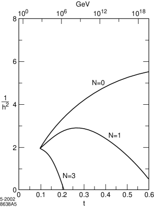
Figure 5: Running of the top-quark Yukawa coupling for $N=0,1,$ and 3.

We see that for the flavor-symmetry option, $N=3$, the heavy quarks, top quarks, and Higgs bosons will be strongly coupled to each other at an energy scale $\sim 10^{3}\ TeV$. We therefore find a new-physics oasis in the desert at this energy scale. However, for the hierarchy option, $N=1$, this does not appear to occur, and the picture remains qualitatively similar to the minimal standard model.

We again emphasize that the Higgs sector becomes strongly coupled at a scale no larger than that for the quarks. If $h^{2}$ approaches infinity, i.e. into strong coupling, then the quartic coupling $\lambda$ gets pulled with it. There is a special separatrix solution, for which the quartic coupling at large values is in proportion to $h^{2}$:

$$\lambda=Kh^{2}\quad(h^{2}\gg g^{2})$$ (108)

with $K$ determined by the solution of

$$4K^{2}+(1+2N)K-4(N+1)=0\ .$$ (109)

This gives

$$K=\left\{\begin{array}[]{rc}0.88&N=0\\ 1.09&N=1\\ 1.31&N=3\end{array}\right\}=1.1\pm 0.2\ .$$ (110)

If $\lambda$ is larger than this critical value, then the Higgs sector can become strong at a scale less than where the top + heavy-fermion sector gets strong. If $\lambda$ is much smaller, then it is driven through zero and to negative values, leading to the unsatisfactory physics of metastable or unstable vacuum. This is shown in Fig. 6. The $N=0$ case in Fig. 6(a) represent the standard model, within the approximations we have made. Note that we obtain a value of $m_{H}=180\pm 20\ GeV$ for the stability corridor, within which the standard model remains perturbative up to the GUT scale. This value is higher by 20 GeV than the results of more sophisticated analyses [30]. The difference is our fault; we have made several simplifications in the renormalization-group equations.

Figure 6: Region of $m_{H},t$ space where the theory remains perturbative: (a) $N=0$ (standard model); (b) $N=1$; (c) $N=3$.

The hierarchical case, $N=1$, shown in Fig. 6(b), is qualitatively similar. The stability corridor is narrower, and its center has moved upward by 5 GeV. In the flavor-symmetric case, $N=3$, shown in Fig. 6(c), the stability corridor terminates at the oasis energy scale of 1000 $TeV$, where strong coupling, or some other modification beyond the contents of this model, is required.

In any case, the conclusion is that if at least some of the new quarks have couplings to the Higgs boson equal to (or greater than) that of the top quark, then their couplings, as well as the Higgs self-coupling itself, get strong at an energy scale small compared to the GUT scale. At higher energy scales the Higgs degree of freedom need not exist at all, something perhaps welcome from the point of view of the hierarchy problem and the fine-tuning (or doublet triplet splitting) problem in dealing with the Higgs as part of a GUT multiplet. This feature makes this “strong coupling” case an interesting hypothesis to investigate in greater detail.

5.2 Running of the gauge couplings

The modifications to the renormalization-group equations for the gauge bosons is straightforward. We have

$$\frac{d}{dt}\left(\frac{1}{g_{3}}\right)^{2} = \left(11-\frac{2}{3}\cdot 6\right)=7\qquad\Rightarrow\qquad\left(11-\frac{2}{3}\cdot 9\right)=5$$

$$\frac{d}{dt}\left(\frac{1}{g_{2}}\right)^{2} = \frac{22}{3}-\frac{1}{3}\,\left[12+\frac{1}{2}\right]=\frac{19}{6}\qquad\Rightarrow\qquad\frac{22}{3}-\frac{1}{3}\,\left[18+\frac{1}{2}\right]=\frac{7}{6}$$

$$-\frac{d}{dt}\left(\frac{1}{g^{\prime}}\right)^{2} = \frac{4}{3}\,\left[5+\frac{1}{8}\right]=\frac{41}{6}\qquad\Rightarrow\qquad\frac{4}{3}\,\left[\frac{15}{2}+\frac{1}{8}\right]=\frac{61}{6}\ .$$ (111)

In the above equations, the first term in each of the square brackets is the fermion contribution, and the second term is the Higgs contributions. Our normalization of $g^{\prime}$ is such that for $SU(5)$ unification

$$\left(\frac{1}{g^{\prime}}\right)^{2}\Rightarrow\frac{3}{5}\ \left(\frac{1}{g_{1}}\right)^{2}\ .$$

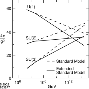
Figure 7: The running of the gauge coupling constants.

With these changes we may compare the one-loop coupling-constant evolution before and after the change. This is shown in Fig. 7.

We see that the three couplings converge somewhat better than in standard $SU(5)$, but not as well as in the MSSM.

6 Outlook

The model we have described has been constructed in a relatively unforced way. We began by assuming that the structure of the mass and mixing matrices were simple and perturbative. This led reasonably naturally to the hypothesis that this simplicity reflected a simple mixing pattern occurring only in the down-quark sector, one that led to a suggestive albeit not compelling right-angle structure of the unitarity triangle. This in turn led to introduction of heavy down quarks in order to implement the mixing. The constraint of anomaly cancellation then led to the extension to $E(6)$ multiplets for the elementary fermions. Examination of the Higgs sector led to the feature of radiatively induced Mexican-hat structure of the Higgs potential via the new heavy down quarks. In addition, the phenomenology has the feature that flavor and CP violation are infrared, diminishing rapidly with higher energy until an energy scale is reached where the mass terms involving the heavy quark sector become dynamical.

All of this we find conceptually attractive. And the story may not end at this point. There is an especially interesting extension associated with the hierarchical choice of new Higgs couplings, as discussed in the previous section. If that choice is made, there exists a parity symmetry within the Higgs sector, broken only by the parity violating electroweak gauge symmetry. To see this we need only invoke the $SU(3)\times SU(3)\times SU(3)$ breakdown of $E(6)$ [31], where the quark nonets are

$$q_{L}=\left(\begin{array}[]{c}u\\ d\\ D\end{array}\right)_{L}\qquad q_{R}=\left(\begin{array}[]{c}u\\ D\\ d\end{array}\right)_{R}\ .$$ (112)

In this notation, Eqs. (21) and (26) become

$${\cal L}^{\prime}=\sum^{3}_{i=1}\overline{q}^{i}_{L}\Phi\left(\begin{array}[]{cc}h_{i}&0\\ 0&H_{i}\end{array}\right)\,q^{i}_{R}+\mbox{h.c.}$$ (113)

where the Higgs field and explicitly shown matrix both act in the upper $2\times 2$ block. With the hierarchical assumption

$$h_{i}=H_{i}\$$ (114)

we see that the Higgs part of the action is parity invariant in the absence of the mass terms. So, ignoring the corrections coming from the parity-violating electroweak gauge symmetry, parity conservation becomes restored at energies large compared to the mass scale of the heavy down-quarks. Note also that all the mass-mixing terms are encapsulated neatly within a ($3,\overline{3}$) Higgs representation:

$$M_{ij}=\left(\begin{array}[]{ccc}h_{i}v&0&0\\ 0&h_{i}v&M_{i}\\ 0&M_{i}&\mu_{ij}\end{array}\right)\ .$$ (115)

The identification of the new heavy-Higgs couplings with the light-Higgs couplings leads to additional constraints on masses and mixings. For example, from Eqs. (24) and (26), we have

$$m_{ij}=\frac{H_{i}v}{M_{i}}\,\mu_{ij}=h_{i}v\left(\frac{\mu_{ij}}{M_{i}}\right)\ .$$ (116)

Therefore

$$\frac{m_{d}}{m_{u}} = \frac{\mu_{11}}{M_{1}}=1.8$$

$$\frac{m_{s}}{m_{c}} = \frac{\mu_{22}}{M_{2}}=0.12$$ (117)

$$\frac{m_{b}}{m_{t}} = \frac{\mu_{33}}{M_{3}}=0.03\ .$$

We are assuming that the off-diagonal flavor mixing effects are perturbative, so that the diagonal elements of the mass matrix are in fact the measured masses. The off-diagonal elements are known in terms of diagonal elements:

$$\frac{\mu_{ij}}{\mu_{ii}}=\frac{m_{ij}}{m_{ii}}\ .$$ (118)

From the estimates in Eq. (15), we obtain

$$\left|\frac{\mu_{12}}{\mu_{11}}\right| = \frac{35\ \mbox{MeV}}{7\ \mbox{MeV}}\approx 5$$

$$\left|\frac{\mu_{13}}{\mu_{11}}\right| = \frac{15\ \mbox{MeV}}{7\ \mbox{MeV}}\approx 2$$ (119)

$$\left|\frac{\mu_{23}}{\mu_{22}}\right| = \frac{m_{23}}{m_{22}}\approx 1.2\ .$$

Actually these relations are completely general.

Now we have demanded that (Eq. (96))

$$M_{3}\buildrel<\over{{}_{\sim}}10\ \mbox{TeV}$$ (120)

so that

$$\mu_{33}=0.03\,M_{3}\leq 300\ \mbox{GeV}\ .$$ (121)

But (cf. Eq. (103))

$$\mu_{11}\approx 1.8\,M_{1}\geq(1.8)(130\,\mbox{GeV})=240\,\mbox{GeV}$$ (122)

implying that the three diagonal $\mu_{ii}$ are almost the same. This suggests

$$M_{2}=\frac{\mu_{22}}{0.12}\sim 2\,\mbox{TeV}\ .$$ (123)

Assuming here that the $\mu_{ii}$ are exactly the same

$$\mu_{ii}\cong 300\,\mbox{GeV}\equiv\mu\qquad\qquad i=1,2,3$$ (124)

leads to a mass matrix with corrections which go beyond our perturbation theory assumptions. To see this, write

$$M^{\prime}_{ij}=\frac{m_{i}}{M_{i}}\,\mu_{ij}=\frac{m_{i}\mu}{M_{i}}\,u_{ij}$$ (125)

with

$$u_{ij}=\frac{\mu_{ij}}{\mu_{ii}}=\frac{\mu_{ij}}{\mu}\ .$$ (126)

Then the square of $M^{\prime}$ is

$${\cal M}^{\prime^{2}}_{ij}=\left(M^{\prime}M^{{\prime}^{\dagger}}\right)_{ij}=m_{ii}m_{jj}u_{ik}u^{*}_{jk}$$ (127)

and we see that

$$({\cal M}^{\prime^{2}})_{ii}=(m_{ii})^{2}\left[1+\sum_{k\neq i}|u_{ik}|^{2}\right]\gg m^{2}_{ii}\ .$$ (128)

Therefore we need to start from scratch and study the diagonalization with much greater care. This does not imply an unworkable scenario, only one which goes in a somewhat different direction than what we have heretofore set up. Going further, however, is left for future work.

7 Conclusions

The main features for experiment of this model are as follows:

1. The possibility of “Stech texture” for the mass matrix, leading to an approximate right angle ($\gamma$) in the unitarity triangle.

2. The existence of three generations of heavy electroweak-singlet down- quarks which decay into their light counterparts plus $W$, $Z$, or Higgs. The masses should be no larger than roughly 10 TeV. The leptons most reasonably are a factor two or so lighter than their heavy-quark counterparts. The first generation quark masses may be near the experimental bound, which is 130 GeV.

3. Flavor and CP violation are induced only by mass-mixing. Therefore above that mass scale, such effects rapidly diminish, only re-emergent if and when the mechanism for the relevant mass terms becomes dynamical. This also implies that radiative-correction effects are in all cases not divergent.

4. Some precision electroweak observables are in principle sensitive to the existence of these new degrees of freedom. The ordinary down quarks and leptons are mixed slightly with their heavy counterparts, making them to not transform as pure doublets or singlets. This leads to nonuniversality of the asymmetries measured in electron-positron annihilation processes. On the other hand, a variety of one-loop radiative correction effects in the down-quark or lepton sectors vanish. No significant corrections, for example, are expected in mass mixing of kaons or neutral $B$’s, nor in $\epsilon$ and $\epsilon^{\prime}$, nor in $b\rightarrow s\gamma,\mu\rightarrow e\gamma$, and $K_{L}\rightarrow\mu e$, nor in the unitarity triangle. There can be significant effects in the up-quark sector, e.g. in $D^{0}-\overline{D^{0}}$ mixing.

5. If the Higgs couplings to the heavy quarks are flavor universal, and at least as large as the Higgs coupling to the top quark, then there will be an oasis in the desert, at an energy scale of about 1000 TeV, where the Higgs, top-quark, and heavy down-quark couplings all become strong. Additional new physics is then assured above this energy scale.

6. If the Higgs couplings to the new quarks are hierarchical, then there need be no oasis. If it is postulated that none exists, the Higgs boson must have a mass of 160 $\pm$ 20 GeV.

References

- [1] See, for instance, Dynamics of Standard Model, J. F. Donoghue, E. Golowich, and B. Holstein, Cambridge University Press (1994).
- [2] See, for instance, S. Weinberg, Quantum Theory of Fields, Vol. III on Supersymmetry, Cambridge University Press (2000).
- [3] R. Sekhar Chivkula et al., in Electroweak Symmetry Breaking and New Physics at the TeV Scale, Ed. T. Barklow et al., World Scientific (1996), p. 352.
- [4] H. Georgi and S. L. Glashow, Phys. Rev. Lett. 32, 438 (1974); H. Georgi, H. Quinn, and S. Weinberg, Phys. Rev. Lett. 33, 451 (1974); J. C. Pati and A. Salam, Phys. Rev. D10, 275 (1974).
- [5] G. ’t Hooft, Lectures at Cargese Summer Institute (1979).
- [6] See, for example, S. Weinberg, Rev. Mod. Phys. 61, 1-23 (1989).
- [7] Much of the material in this paper overlaps with J. D. Bjorken, The Gaugeless Limit of the Electroweak Theory, Oxford Lectures (1996); and can be found at http://www-th.phys.ox.au.uk/users/ProfBjorken/home.html and a more detailed exegesis is given there.
- [8] S. Weinberg, Phys. Rev. D19, 1277 (1979); L. Susskind, Phys. Rev. D20, 2619 (1979).
- [9] E. Eichten and K. Lane, Phys. Lett. B90, 125 (1980).
- [10] H. Fritzsch, hep-ph/9605388; H. Fritzsch and Z.-Z. Xing, Nucl. Phys. B556, 49 (1999).
- [11] D. Hawkins and D. Silverman, hep-ph/0205011, and references therein.
- [12] F. Gürsey, P. Ramond, and P. Sikivie, Phys. Lett. 60B, 177 (1976); J. Hewett and T. Rizzo, Phys. Rept. 183, 196 (1989).
- [13] Y. Nambu, Proceedings of the 1988 Kasimierz Workshop, Z. Adjuk et al. Ed., (World Scientific 1989); W. Bardeen, C. Hill, and M. Lindner, Phys. Rev. D41, 1647 (1990); V. Miransky, M. Tanabashi, and K. Yamawaki, Mod. Phys. Lett. A4, 1043 (1989).
- [14] N. Cabibbo, Phys. Rev. Lett. 12, 62 (1963).
- [15] M. Kobayashi and T. Maskawa, Prog. Theoret. Phys. 49, 652 (1973).
- [16] B. Stech, Phys. Lett. 130B, 189 (1983).
- [17] The BELLE Collaboration: K. Abe et al., Phys. Rev. Lett. 87, 091802 (2001); The BaBar Collaboration: B. Aubert et al., ibid 87, 091801 (2001).
- [18] The current status of measurement of is that a value of is ruled out. But a within a few % of 1 is certainly allowed; see e.g. the review of the CKM matrix in the 2002 version of PDG: K. Hagiwara et al. (Particle Data Group) Phys. Rev. D66, 010001 (2002).
- [19] Z. Maki, M. Nakagawa, and S. Sakata, Prog. Theoret. Phys. 28, 870 (1962).
- [20] This is obtained from an analysis of decaying into jets by the DØ Collaboration; see e.g. Ref. [21].
- [21] Review of Particle Physics, The European Physical Journal 15, 1 (2000).
- [22] K. Babu et al, Phys. Lett. 205B, 540 (1988); G. Branco et al., Phys. Rev. D52, 4217 (1995).
- [23] M. Peskin and T. Takeuchi, Phys. Rev. D46, 385 (1992).
- [24] G. Altarelli, R. Barbieri and S. Jadach, Nucl. Phys. B369, 3 (1992).
- [25] J. Hewett, hep-ph/9810316, Proceedings of TASI 97, Supersymmetry, Supergravity and Supercolliders, Boulder, CO.
- [26] J. Leveille, Nucl. Phys. B137, 63 (1977).
- [27] T. Rizzo, Phys. Rev. D33, 3329 (1986).
- [28] J. Hewett, T.G. Rizzo and J.A. Robinson, Phys. Rev. D33, 1476 (1986). It is shown here that if is broken in the pattern then has the value + 18.
- [29] T. Appelquist and J. Carazzone, Phys. Rev. D11, 2856 (1975).
- [30] See for example, C. Quigg, Acta Phys. Polonica, B30, 2145 (1999). K. Riesselmann, DESY-97-222, Talk given at International School of Subnuclear Physics, 35th Course: Highlights: 50 Years Later, Erice, Italy, 26 Aug–4 Sep 1997. In Erice 1997, Highlights of subnuclear physics pp. 584-592; hep-ph/9711456.
- [31] Similar assignments have been considered before. R. W. Robinett and J. Rosner, Phys. Rev. D26, 2396 (1982); D. London and J. Rosner, Phys. Rev., D34, 1530 (1986); D. Chang and R. N. Mohapatra, Phys. Lett B175, 304 (1986).