Physics of Event Generators

Abstract

An event generator for nuclear collisions is a microscopic model, obtained from extrapolating elementary interactions – as electron-positron annihilation, deep inelastic scattering, and proton-proton interactions – towards proton-nucleus and nucleus-nucleus scattering, by using Monte Carlo techniques.

In this paper, we will discuss the physical concepts behind such event generators. We first present some qualitative discussion of nuclear scattering, before discussing particle production and strings. We then discuss the parton model, and finally multiple scattering theory.

SUBATECH, Universit de Nantes – IN2P3/CNRS – EMN, Nantes, France

1 Qualitative Discussion of Nuclear Scattering

1.1 Overview

Relativistic nuclei are Lorentz contracted, which means that the longitudinal dimension $2R$ is reduced to $2R/\gamma$, see fig. 1,

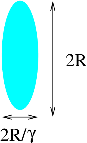
Figure 1: Nuclei are Lorentz contracted.

where $R$ is the nuclear radius, and $\gamma=1/\sqrt{1-(v/c)^{2}}$ the so-called gamma factor. At the heavy ion collider RHIC, we have $\gamma=100$ and at LHC about $\gamma=3000$, so relativistic contraction plays a very essential role.

Considering the collision of two nuclei, there are first of all the primary interactions, when the two nuclei pass trough each other in a very short time, see fig 2.

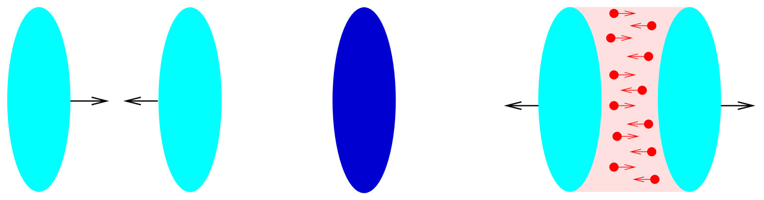
Figure 2: Nuclei pass through each other in a very short time.

Since at very high energies the longitudinal size is due to the gamma factor almost zero (of the order of 0.1 fm at RHIC and 0.01 fm at LHC), all the nucleons of the projectile interact with all the nucleons of the target instantaneously. Many elementary interactions between nucleons in the two nuclei happen in parallel, resulting in many partons (quarks and gluons), moving mainly in longitudinal direction (pre-equilibrium). These partons interact

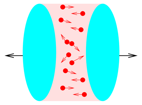
Figure 3: The partons interact and finally reach equilibrium (QGP).

and finally reach equilibrium, referred to as quark-gluon plasma (QGP). The system then expands, passing via a phase transition (or sudden crossover) into the hadronic phase. The density decreases further till the collision rate is no longer large enough to maintain chemical equilibrium, but there are still hadronic interactions till finally the particles “freeze out”, i.e. they continue their way without further interactions.

Unfortunately there does not exist a single formalism being able to account for a complete nucleus-nucleus collision. Rather we have - at least for the moment - to divide the reaction into different stages, and try to understand the different stages as good as possible. These different stages are

• Initial stage,

• Pre-equilibrium stage,

• Quark-gluon plasma,

• Phase transition,

• Hadron gas,

• Non-equilibrium hadronic matter,

• Free hadrons.

Before discussing these stages one after the other, we introduce some useful variables, as there are the proper time $\tau$ and the space time rapidity $\eta$

$$\tau=\sqrt{t^{2}-z^{2}},\qquad\eta=\frac{1}{2}\ln\frac{t+z}{t-z},$$

and the transverse mass $m_{t}$ and the rapidity $y$

$$m_{t}=\sqrt{E^{2}-p_{z}^{2}},\qquad y=\frac{1}{2}\ln\frac{E+p_{z}}{E-p_{z}}.$$

The proper time and the transverse mass have the property to be invariant under Lorentz transformations. The (space time) rapidity is additive under Lorentz boosts.

Knowing that constant proper time represents hyperbolas in space-time ($t-z)$, one may present a space-time picture of the different stages of heavy ion collisions, as shown in fig. 4.

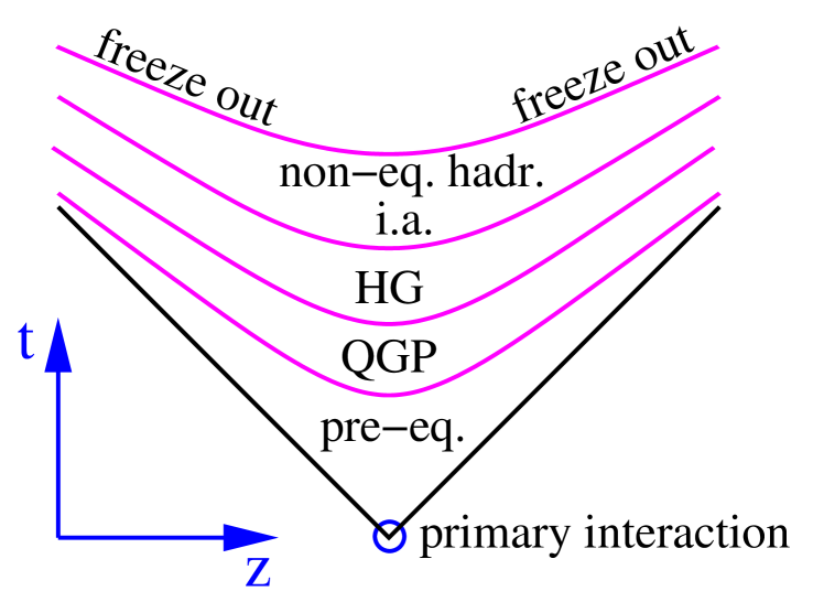
Figure 4: The different stages of heavy ion collisions.

1.2 Initial Stage

The understanding of the initial interactions is crucial for any theoretical treatment of a possible parton-hadron phase transition, the detection of which being the ultimate aim of all the efforts of colliding heavy ions at very high energies. Theoretical approaches have to consider the fact that the nuclear collision happens on a very short time scale, such that all nucleons of the target interact with all nucleons of the projectile practically instantaneous, see fig. 5.

Figure 5: The initial stage of heavy ion collisions.

It is quite clear that coherence is crucial for the very early stage of nuclear collisions, so a real quantum treatment is necessary and any attempt to use a transport theoretical parton approach with incoherent quasi-classical partons should not be considered at this point. Also semi-classical hadronic cascades cannot be stretched to account for the very first interactions, even when this is considered to amount to a string excitation, since it is well known [1] that such a longitudinal excitation is simple kinematically impossible.

So what are the currently used fully quantum mechanical approaches? There are presently considerable efforts to describe nuclear collisions via solving classical Yang-Mills equations, which allows to calculate inclusive parton distributions [2]. This approach is to some extent orthogonal to ours: here, screening is due to perturbative processes, whereas we claim to have good reasons to consider soft processes to be at the origin of screening corrections.

Provided factorization works for nuclear collisions, on may employ the parton model, which allows to calculate inclusive cross sections as a convolution of an elementary cross section with parton distribution functions, with these distribution functions taken from deep inelastic scattering. Parton model based are for example Pythia [3] and HIJING [4].

Another approach is the so-called Gribov-Regge theory. This is an effective field theory, which allows multiple interactions to happen “in parallel”, with the phenomenological object called “Pomeron” representing an elementary interaction. Using the general rules of field theory, on may express cross sections in terms of a couple of parameters characterizing the Pomeron. A disadvantage is the fact that cross sections and particle production are not calculated consistently: the fact that energy needs to be shared between many Pomerons in case of multiple scattering is well taken into account when calculating particle production (Monte Carlo applications), but energy conservation is not taken care of for cross section calculations. Models based on this approach are QGS [5], DPM [6, 7], and VENUS [8].

A new approach, called “Parton-based Gribov-Regge Theory” [1], solves some of the above-mentioned problems: one has a consistent treatment for calculating cross sections and particle production, considering energy conservation in both cases; one introduces hard processes in a natural way, and, compared to the parton model, one can deal with total cross sections without arbitrary assumptions. This model is incorporated in the NEXUS [1] event generator.

1.3 Pre-equilibrium Stage

The partons created in the primary interactions are certainly far from equilibrium, and is desirable to understand microscopically the equilibrium of the system, in other words the formation of a quark gluon plasma. This is a difficult task, since for example at RHIC energies there is still a large soft component. Nevertheless it is useful to study the evolution of partonic systems based on pQCD, ignoring soft physics.

The theoretical tool for this stage is the “parton cascade”, which amounts to considering partons as classical particles which move on straight line trajectories, where binary interactions are defined via parton-parton cross sections calculated in the framework of perturbative QCD [9], see fig. 6.

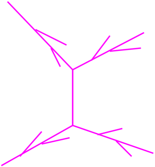
Figure 6: Partons, which have been produced initially, interact.

One has to carefully regard the range of validity of this approach: it is not meant to treat the primary interactions, where quantum mechanical interference should play a crucial role, so one may start the calculation once a system of incoherent classical partons has been established. On the other end, one should not stretch the perturbative treatment too far: perturbative calculations require large momentum transfer, which is not any more guaranteed if the interaction energy is getting too low.

1.4 Equilibrium Stage

We are now discussing the final stage of the collision, consisting of the QGP phase, the phase transition, and the hadron gas phase. We do not treat these three stages individually, because the known models treat usually more than just one stage.

The final aim of all the efforts in the field of ultra-relativistic heavy ion collisions is the creation of a thermalized system of quarks and gluons. Provided such an equilibrium has been established, one may use hydrodynamics, which is a macroscopic approach based on energy-momentum conservation and local thermal equilibrium. Hydrodynamical calculations have been used since a long time, either assuming particular symmetries and using analytical methods [10], or full 3-dimensional calculations numerical calculations [11]. Recently a new technique has been proposed, the so-called smoothed particle hydrodynamics [12], where fields $\rho(x)$ are represented by particles as $\rho_{P}(x)=\Sigma_{b}\nu_{b}\delta(x-x_{b})$, and then smoothed:

$$\rho(x)\rightarrow\rho_{SP}(x)=\int\rho_{P}(x)W(x-x^{\prime})dx^{\prime}=\Sigma_{b}\nu_{b}W(x-x_{b})$$

with some smoothing kernel W. The advantage is that the hydrodynamical equations are transfered into a system of ordinary differential equations, which can be solved by applying standard methods. In this way one may perform 3-dimensional calculations much faster than with traditional methods.

There are several attempts to treat at least the region around the phase transition in a microscopic way. A possibility is to apply transport theory based on the NJL model [13], which is an effective theory with a point-like interaction between two quarks (gluons are not considered explicitly). The model allows also for hadron production like quark plus anti-quark goes into meson plus meson. The dynamics is crucially affected by the density and temperature dependence of quark and hadron masses, one observes for example the formation of droplets of quark matter rather than homogeneous matter of lower density, since the latter one would imply higher quark masses.

A completely different hadronization scenario has been proposed based on the confinement mechanism [14], again ignoring gluons. Quarks are considered to be classical particles, their dynamics being determined by a classical Hamiltonian. The latter one contains a string potential and color factors, which force the quarks to form resonances, which subsequently decay into hadrons.

Another alternative approach is the hadronization via coalescence [15]. Again, starting from a quark-anti-quark plasma, hadronic resonances are formed based on coalescence, with a subsequent decay into hadrons.

1.5 Post-equilibrium Hadronic Stage

Once a purely hadronic system has been established, a microscopic treatment based on binary hadronic interactions is feasible. Here, hadrons propagate on classical trajectories and interact according to hadron-hadron scattering cross sections. If possible, parameterizations of measured cross sections are used. A couple of models have been constructed along these lines, like UrQMD [16, 17], ART [18], JAM [19]. Unfortunately, not all the necessary cross sections have been measured to a sufficient precision, and correspondingly, the above-mentioned approaches differ by using different model assumptions for the cross sections. We emphasize again that hadronic transport codes are a useful tool to treat the final stage of a heavy ion collision, but not for the primary interaction.

2 Particle Production, Strings

Particle production is relevant for $pp$, $pA$ and the initial stage of $AA$ collisions. However it is necessary to first study simpler systems as electron-positron annihilation.

2.1 The String Picture

For $e^{+}e^{-}$ collisions, we have data available in a wide energy range (up to 200 GeV in the cms). Studying particle production, one observes (idealized) a rapidity plateau, see fig. 7.

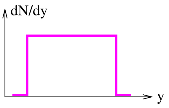
Figure 7: One observes (idealized) a rapidity plateau.

When we move the reference system (for example from lab to rest frame), we observe a manifestation of boost invariance: the same rapidity distribution before and after the boost, see fig 8.

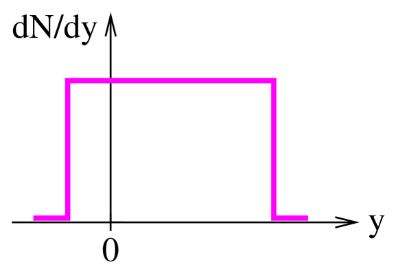
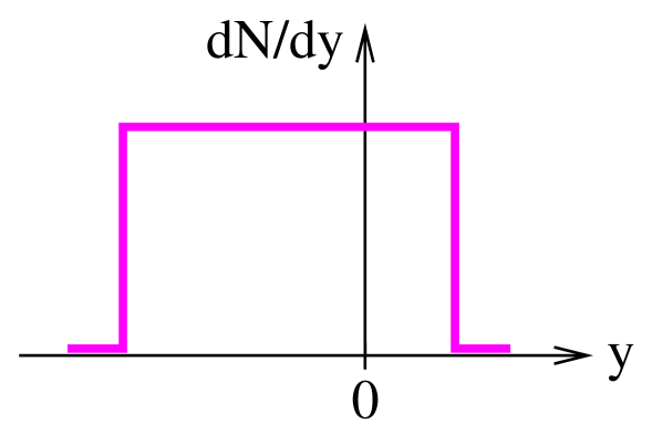
Figure 8: Manifestation of boost invariance

What does boost invariance mean? Suppose an expanding dynamical system such that some central part is at rest and the outer parts move away from the center, with increasing speed for larger distances, see fig. 9(left).

      

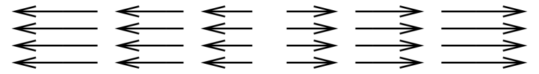
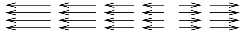
Figure 9: Manifestation of boost invariance

Now we perform a boost such that a different piece of the system is at rest. In the neighborhood of this region the system looks identical to the neighborhood of the point at rest before the boost, see fig. 9(right). In other words: the system is identical at all points in the corresponding local comoving frame.

What happens really? Electron and positron annihilate and form a virtual photon, then the virtual photon decays into a quark-antiquark pair, see fig. 10(a). The quark and antiquark move apart from each other, see fig. 10(b). But quarks and antiquarks cannot be observed individually! There is a gluon field acting between the two, whose energy is proportional to the separation distance. This object is called string, see fig. 11.

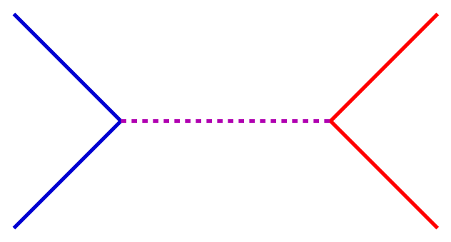
(a)        (b)

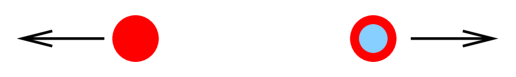
Figure 10: (a) Electron and positron annihilate and form a virtual photon, then the virtual photon decays into a quark-antiquark pair. (b) Quark and antiquark move apart from each other.

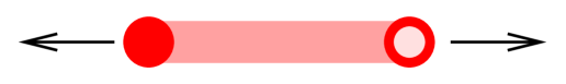
Figure 11: The quark-antiquark pair forms a string.

To separate the quark from the antiquark, one need an infinite energy, which is impossible. The string breaks via quark-antiquark production, and these new string pieces are finally hadrons or resonances, see fig. 12.

Figure 12: The string breaks via "quark-antiquark" production.

String fragmentation is a boost invariant procedure and provides exactly the situation discussed above: seen from a given point on the string, all the string pieces move away from this point with increasing speed towards the edges, as indicated in fig. 13. In fig. 14,

before:  after:

Figure 13: String fragmentation is a boost invariant procedure.

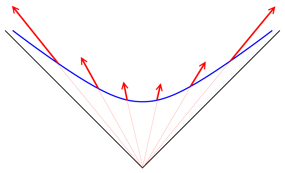
Figure 14: Space-time picture of string decay.

we present the space-time picture of the string dynamics: at given proper time (hyperbola), the velocities of the string pieces (arrows) are such that they point all back to the origin and are longer towards the edges. This string decay provides a flat rapidity distribution.

2.2 What is Really Done

After this qualitative discussion, let us discuss what is really done. A string can be considered as a two-dimensional surface in Minkowski space

$$X=X(r,t),$$

with $r$ being a space-like and $t$ a time-like parameter, see fig. 15.

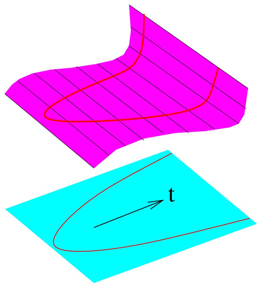
Figure 15: The string surface.

In order to obtain the equations of motion, we need a Lagrangian. It is obtained by demanding the invariance of the action with respect to gauge transformations. This way one finds [1] the Lagrangian of Nambu-Goto:

$$L=-\kappa\sqrt{(X^{\prime}\dot{X})^{2}-X^{\prime 2}{\dot{X}}^{2},}$$

with “dot” and “prime” referring to the partial derivatives with respect to $r$ and $t$, and with $\kappa$ being the string tension. With this Lagrangian we get the Euler-Lagrange equations of motion:

$$\frac{\partial}{\partial t}\frac{\partial L}{\partial\dot{X}_{\mu}}+\frac{\partial}{\partial r}\frac{\partial L}{\partial X^{\prime}_{\mu}}=0.$$

We use the gauge fixing

$$X^{\prime 2}+{\dot{X}}^{2}=0\>\mathrm{and}\>X^{\prime}\dot{X}=0,$$

which provides a very simple equation of motion, namely a wave equation,

$$\frac{\partial^{2}X_{\mu}}{\partial t^{2}}-\frac{\partial^{2}X_{\mu}}{\partial r^{2}}=0,$$

with the boundary conditions: $\partial X_{\mu}/\partial\sigma=0,\>\sigma=0,\pi$. The solution of the equation of motion (with initial extension zero) is

$$X^{\mu}(r,t)=X_{0}+\frac{1}{2}\left(\int_{r-t}^{r+t}g^{\mu}(\xi)d\xi\right),$$

where $g$ is the initial velocity, $g(r)=\dot{X}(r,t)_{t=0}$ . Strings are classified according to the function $g$. Strings with piecewise constant $g$ are called kinky strings, each segment being called kink, finally identified with perturbative partons. In fig. 16, we show the evolution of a string generated in electron-positron annihilation (3 internal kinks).

Figure 16: String evolution.

2.3 Results

We show some results for rapidity distributions from flat strings (no internal kinks) in fig. 17. We observe a nice rapidity plateau, which gets broader with increasing energy. But the plateau height stays constant. Increasing the energy does not change the local properties of the string, the number of particles per unit of rapidity stays constant.

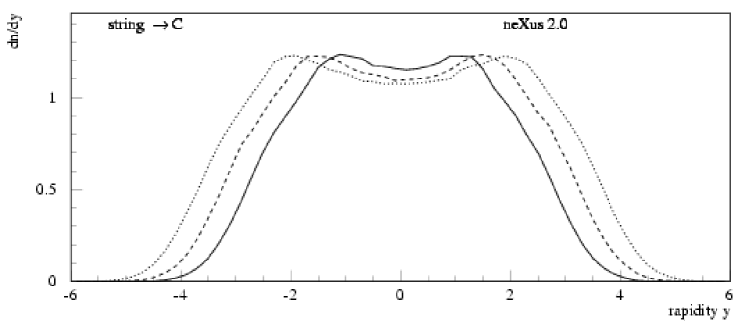
Figure 17: Rapidity distributions of flat strings at 14-22-34 GeV.

In real $e^{+}e^{-}$ collisions, one has with increasing energy an increasing probability to have kinks, which makes the plateau rising with energy, as shown in fig. 18, where we show the prediction of the string model together with experimental data from the TASSO [20], ALEPH [21], and OPAL [22, 23] collaborations. We show also longitudinal momentum fraction distributions for different energies.

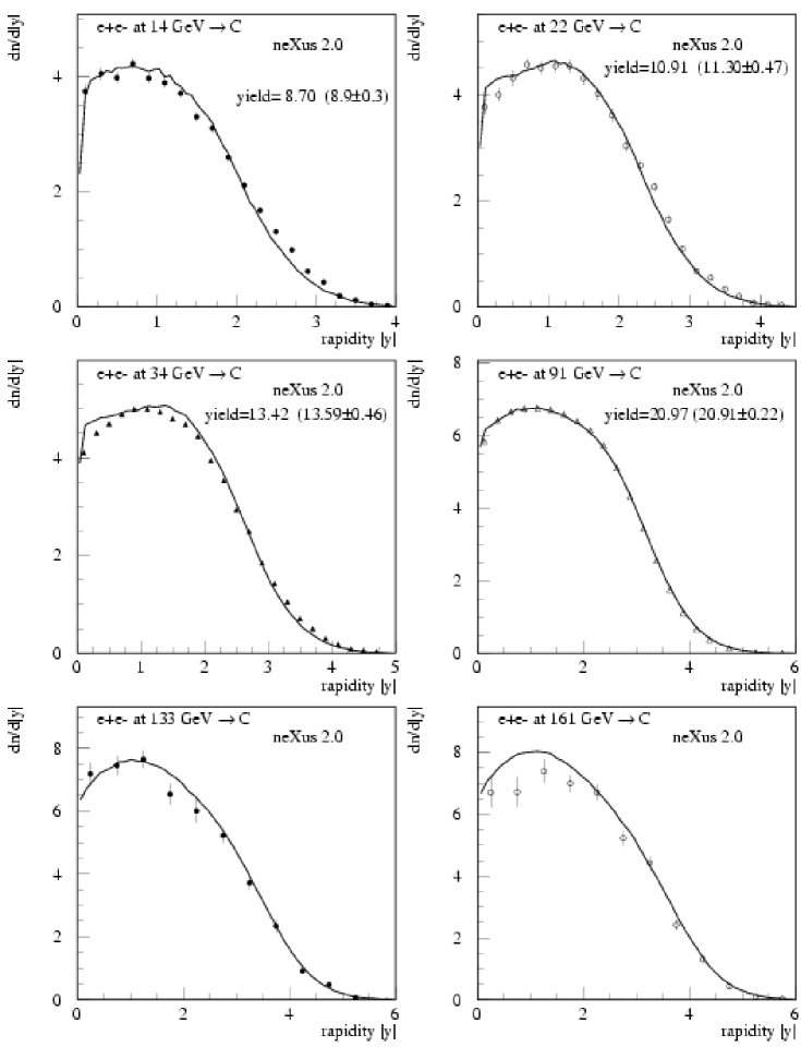
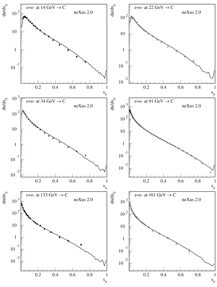
Figure 18: Rapidity and longitudinal momentum distributions: data (points) and NEXUS (line).

2.4 Hadron Flavors

There are some remarkable regularities among the hadrons, which became apparent in the early 1960s. The first is that the baryons fall into groups of multiplicity 1, 8, 10 (singlet, octet, decuplet). The mesons come in singlets and octets. See figs. 19, 20.

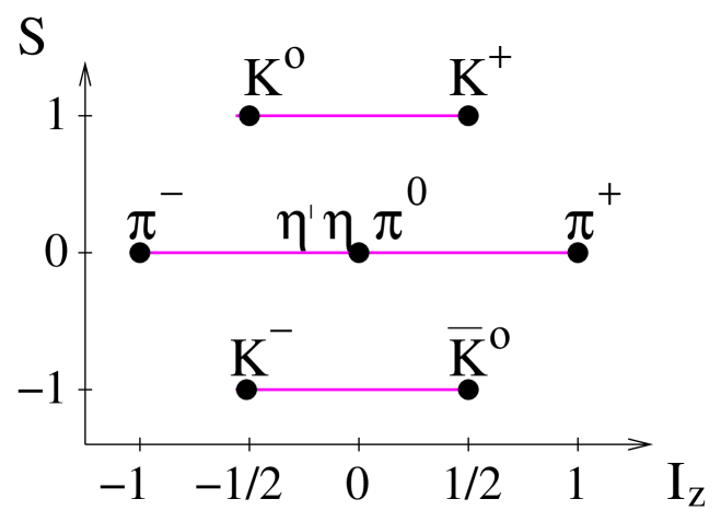
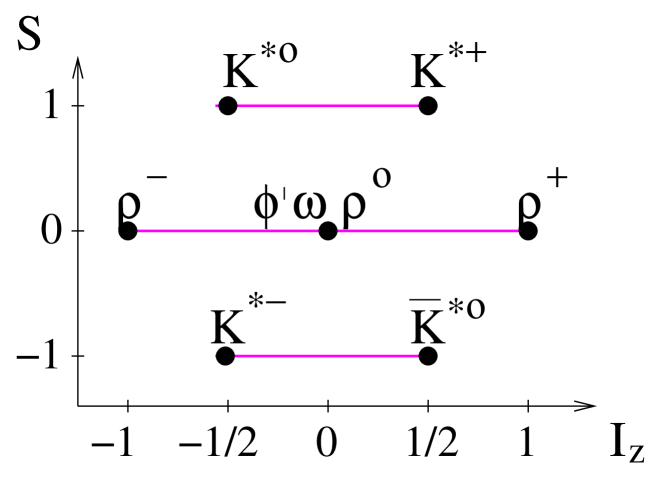
Figure 19: Meson octet plus singlet.

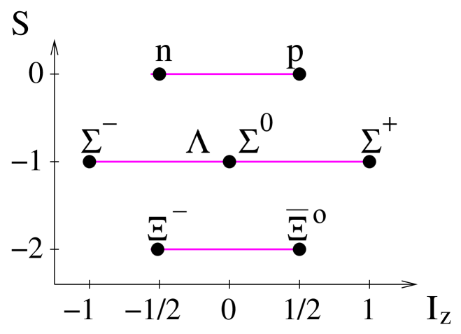
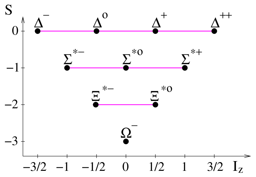
Figure 20: Baryon octet and decuplet.

These structures can be understood in the quark model for hadrons: the baryons are composed of three quarks, the antibaryons of three antiquarks and the mesons of a quark plus an antiquark. There are six flavors of quarks, the three most abundant ones being the $u$, $d$, and $s$ flavor, the properties being given in table 1, shown in fig. 21.

name	u	d	s
charge	2/3	-1/3	-1/3
strangeness	0	0	-1
isospin	1/2	-1/2	0

Table 1: Quark properties.

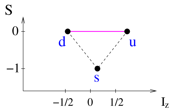
Figure 21: Quark properties.

In figs. 22 and 23, we indicate the quark content of the most frequent mesons and baryons. So the quark model can easily explain the striking regularities of the hadrons.

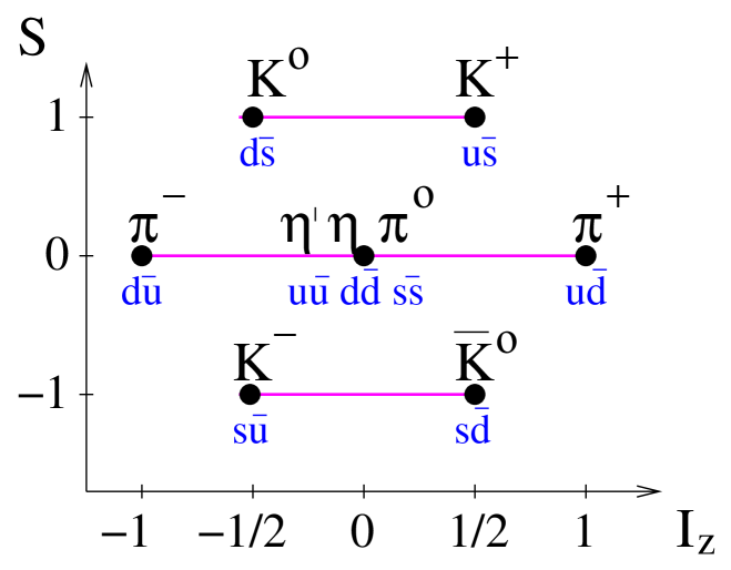
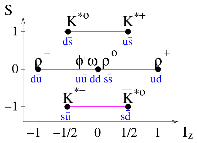
Figure 22: The quark content of mesons.

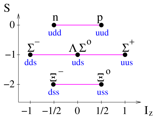
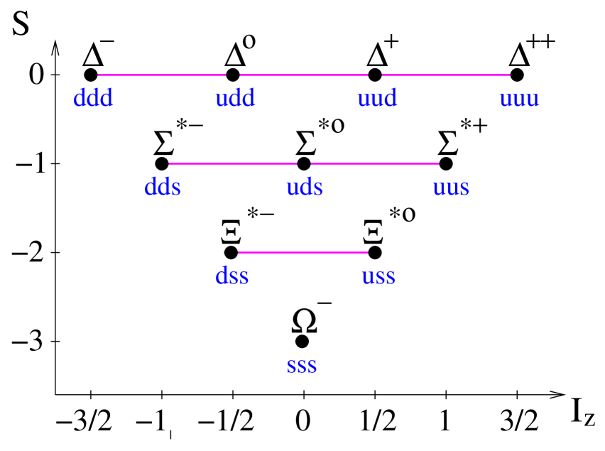
Figure 23: The quark content of baryons.

It will be the basis of all models of string fragmentation, as shown in fig. 24. A string break is realized via quark-antiquark production, such that the quark-antiquark pair screens the color field. The string fragments consist then of quark-antiquark pairs, they are therefore mesons. It is also possible that the string breaks via diquark-antidiquark production, which amounts to baryon and antibaryon creation.In fig. 25, we show some results concerning the production of identified hadrons in electron-positron annihilation. One observes that the string model works to a high precision.

      

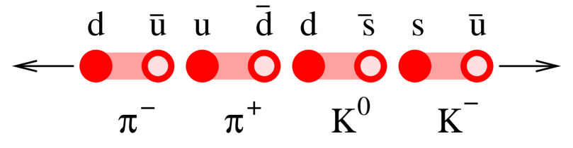
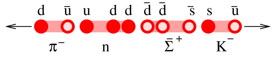
Figure 24: Hadron production from a quark-antiquark string.

Figure 25: Hadron production in $e^{+}e^{-}$ annihilation at 29 and 91 GeV.

3 Parton Model

Whereas leptons are point-like in their behavior, it is not inconceivable that the quarks too enjoy this property. If we think of the hadrons as complicated “atoms” or “molecules” of quarks, then at high energies and momentum transfers, where we are probing the inner structure, we may discover a simple situation, with the behavior controlled by almost free, point-like constituents. The idea that hadrons possess a “granular” structure and that the “granules” behave as hard point-like, almost free (but nevertheless confined) objects, is the basis of Feynmans (1969) parton model.

The essence of the parton model is the assumption that, when a sufficiently high momentum transfer reaction takes place, the projectile, be it a lepton or a parton inside a hadron, sees the target as made up of almost free constituents, and is scattered by a single, free, effectively massless constituent.

3.1 Deep Inelastic Scattering

The historical way to study the hadronic structure was using point-like leptons as projectiles hitting a proton target. There is a basic difference compared to $e^{+}e^{-}$ scattering: the proton is a composite particle, $e^{+}$, $e^{-}$ are elementary particles. so one can probe the internal structure of the proton, see fig. 26(left).

      

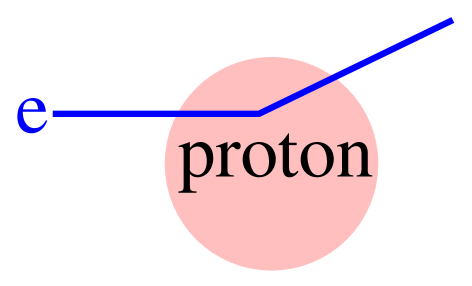
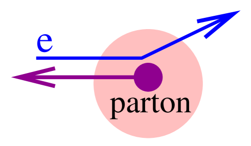
Figure 26: lepton-proton scattering.

In a lepton-proton scattering, one can measure the momentum distributions of constituents (partons) see fig. 26(right). In lowest order of perturbation theory, the reaction is described by one photon exchange diagram, see fig. 27. Here $k$ is known and $k^{\prime}$ is measured, so the momentum transfer $q$ is known.

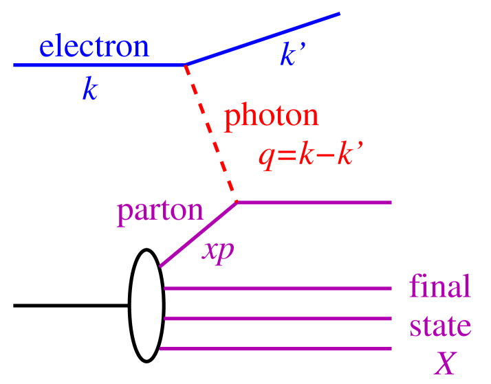
Figure 27: One photon exchange in a $ep$ reaction.

One studies the cross section as function of two variables: the photon virtuality $Q^{2}=-q^{2}$ and the Bjorken variable $x=Q^{2}/2pq.$ Why $Q^{2}$? Because $Q^{2}$ sets the resolution scale: $\Delta x=1/Q^{2}$. The bigger $Q^{2}$ the deeper one looks into the proton. Why x? Consider a parton with a momentum fraction $z$ (momentum $zp$), see fig. 28.

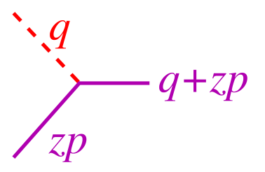
Figure 28: The photon-parton vertex.

In the reaction it received the transferred momentum $q$, so its new momentum is $q+zp$. But the parton is massless, so $q^{2}+2qzp+z^{2}p^{2}=0$, and therefore $z=x$. A reaction with a certain value of $x$ probes a parton with momentum fraction $z=x$, which means that parton momentum distribution are measurable.

Let us do some kinematics: the virtual photon transfer being $q$ and the initial proton momentum being $p$, the final state mass $W$ is given as $W^{2}=(p+q)^{2}$, see fig. 29. We have

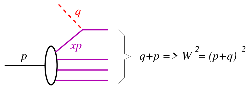
Figure 29: The total mass $W$ of the hadronic final state.

,

$$W^{2}=(q+p)^{2}=q^{2}+2pq+p^{2}\approx-Q^{2}+Q^{2}/x,$$

which gives

$$W^{2}=Q^{2}(\frac{1}{x}-1)$$

So we arrive at an interesting result: small $x$ corresponds to a big final state mass $W$.

One can write the $ep$ cross section as

$$\frac{d\sigma^{ep}}{dQ^{2}dx}=\frac{\alpha}{\pi Q^{2}x}\left[\frac{1+(1-y)^{2}}{2}\sigma_{T}^{\gamma p}+(1-y)\sigma_{L}^{\gamma p}\right],$$

with $y=pq/pk$, and

$$\sigma_{T}^{\gamma p}=\frac{4\pi^{2}\alpha}{Q^{2}}(F_{2}-F_{L}),\sigma_{L}^{\gamma p}=\frac{4\pi^{2}\alpha}{Q^{2}}F_{L},F_{L}\ll F_{2}.$$

$F_{2}$ and $F_{L}$ describe the proton structure as seen by the virtual photon, see fig. 30.

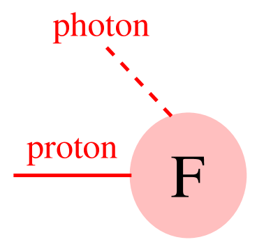
Figure 30: Proton structure functions.

A first look reveals $F_{2}(x,Q^{2})$to be only a function of x (scaling). This can be explained within the naive Parton Model, where the proton is considered to be a incoherent sum of partons (quarks) of flavor $i$, which are distributed according to parton distribution functions $f_{i}$ , so

$$F_{2}(x,Q^{2})=\sum_{i}e_{i}\,x\,f_{i}(x).$$

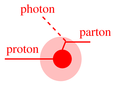
Figure 31: Parton model.

Looking more carefully, on finds that $F_{2}(x,Q^{2})$ depends slightly on $Q^{2}$ (scale breaking). The partons are still distributed according to parton distribution functions $f_{i}(x,Q^{2})$, which are now depending on a scale (defined by the probe). And we still have

$$F_{2}(x,Q^{2})=\Sigma_{i}e_{i}xf_{i}(x,Q^{2}).$$

This formula takes in account the successive emissions of virtual partons, carrying less and less momentum. The photon virtualities, $Q^{2}$, are ordered down to some minimum value (this part is calculable in the framework of perturbative QCD). Below this minimum value, we have soft physics (non-perturbative regime), see fig. 32.

Figure 32: Successive parton emissions.

Let us consider the emission of the first (softest) parton being emitted from the non-perturbative area. If the parton carries a fraction $x$ of the momentum of the proton, the mass of the soft object ”proton minus parton” has a mass given by $m^{2}=Q_{0}^{2}/x$, where $Q_{0}$ is a typical soft virtuality (of the order 1 GeV). This has interesting consequences: in case of sea quarks with distributions of the form $1/x$, one has typically small $x$ and therefore a large mass $m$. For valence quarks, on the other hand, a $1/\sqrt{x}$ distribution provides in general large $x$ values and therefore a small mass $m$. This means that in case of sea quarks, there is a large mass and small virtuality object between the proton and the parton, and we therefore have to consider two contributions to the structure functions, as indicated in fig. 33. The large mass object is considered to be a Pomeron, to be discussed in detail later.

Figure 33: Two contributions for the proton structure function.

The valence contribution provides a peak at large $x$ and drops fast for small values of $x$, whereas the sea contribution is important at small $x$ and drops very fast towards large $x$. The sum of the two is shown in fig. 34.

Figure 34: The structure function $F_{2}$.

3.2 The Parton Model for pp

For $pp$ interactions one uses the same concept as for lepton-proton scattering. Each proton contains partons distributed as $f_{i}(x,Q^{2})$. Two of the partons (one from the first proton and the other from the second proton) interact via elementary interactions. The inclusive cross section for producing a parton k is

$$\frac{d\sigma^{pp\rightarrow k}}{dyd^{2}p_{t}}=\sum_{i,j}\int dx_{1}dx_{2}f_{i}(x_{1},Q^{2})f_{j}(x_{2},Q^{2})\frac{d\hat{\sigma}^{ij\rightarrow k}}{dyd^{2}p_{t}},$$

(see fig. 35), where $f_{i}(x,Q^{2})$ are the perturbative parton densities, measured by performing global fits of data taken from large sets of experiments as lepton-nucleon deep inelastic scattering and others. $d\hat{\sigma}/dyd^{2}p_{t}$ are partonic cross-section for the hard processes, calculable in perturbation theory.

Figure 35: The inclusive cross section for producing partons.

Here, one assumes universality of parton densities (independent of the hard processes, for large $Q^{2}$) and factorization (the possibility to separate the parton density functions from the partonic cross section). The assumption is based in the fact that hard processes ($Q\gg m_{p}$) occur in very short time ($\tau\sim 1/Q$), much lesser than the typical interaction times for the binding of the proton (hadron) ($\tau\sim 1/m_{p}$). As a result, to study inclusive processes at large $Q^{2}$ it is sufficient to consider the interactions between the external probe and a single parton.

The model works well for most of the high energy physics experiments, but diverges for small transverse momentum. Why? Because soft (non-perturbative) physics enters. A solution is to introduce some lower limit (cutoff $p_{0}$) for the transverse momentum. Integrating over rapidity and the transverse momentum above the cutoff, we get the jet cross section $\sigma(p_{0})$. Now another problem appears: the jet cross section grows very fast with energy, becoming finally bigger than the total one, see fig. 36.

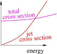
Figure 36: The jet cross section grows very fast with energy .

The real solution amounts to studying multiple scattering. The jet cross section is an inclusive one: several jets may contribute. So the parton model is very useful but is not the whole history. One needs a multiple scattering theory.

There is currently much discussion about saturation. What does it mean? Consider partons with transverse momentum $p_{0}$. Each one occupies a transverse area $\pi/p_{0}^{2}$, whereas the transverse area of the nucleon is $\pi R_{A}^{2}$. If the number $N_{A}(s,p_{0}^{2})$ of partons is sufficiently high, they fill completely the transverse area of the nucleus. The relation

$$N_{A}(s,p_{0}^{2})\pi/p_{0}^{2}=\pi R_{A}^{2}\>\mathrm{or}\>p_{0}^{2}=N_{A}(s,p_{0}^{2})/R_{A}^{2}$$

defines therefore the so-called saturation scale $p_{0}^{2}$. Since $N_{A}(s,p_{0}^{2})$ increases with $s$ and decreases with $p_{0}^{2}$, then the condition $p_{0}^{2}=N_{A}(s,p_{0}^{2})/R_{A}^{2}$ is solved by a function $p_{0}^{2}(s)$ which increases with s, such that at sufficiently high energy the scale $p_{0}^{2}(s)$ in in the perturbative domain.

4 Multiple Scattering Theory

4.1 Reminder: some Elementary Quantum Mechanics

Let us introduce some conventions. We denote elastic two body scattering amplitudes as $T_{2\rightarrow 2}$ and inelastic amplitudes corresponding to the production of some final state $X$ as $T_{2\rightarrow X}$ (see fig.37 ).

      

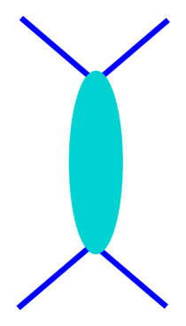
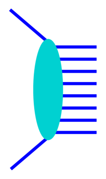
Figure 37: An elastic scattering amplitude $T_{2\rightarrow 2}$ (left) and an inelastic amplitude $T_{2\rightarrow X}$ (right).

As a direct consequence of unitarity on has $2\,\mathrm{Im}T_{2\rightarrow 2}=\sum_{x}$$(T_{2\rightarrow X})$$(T_{2\rightarrow X})^{*}$. The right hand side of this equation may be literally presented as a “cut diagram”, where the diagram on one side of the cut is $(T_{2\rightarrow X})$ and on the other side $(T_{2\rightarrow X})^{*}$, as shown in fig.38 .

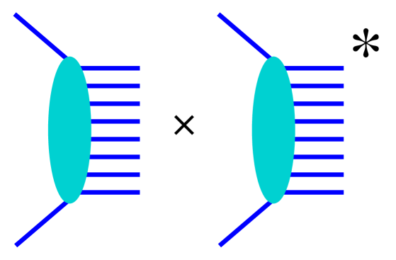
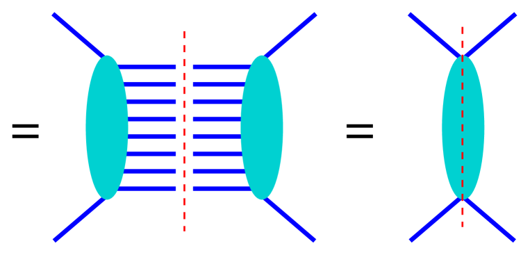
Figure 38: The expression $\sum_{X}(T_{2\rightarrow X}).$$(T_{2\rightarrow X})^{*}$which may be represented as a “cut diagram”.

So the term “cut diagram” means nothing but the square of an inelastic amplitude, summed over all final states, which is equal to twice the imaginary part of the elastic amplitude. Based on these considerations, we introduce simple graphical symbols, which will be very convenient when discussing multiple scattering, shown in fig. 39: a vertical solid line represents an elastic amplitude (multiplied by $i$, for convenience), and a vertical dashed line represents the mathematical expression related to the above-mentioned cut diagram (divided by $2s$, for convenience).

      

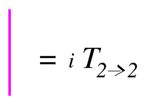
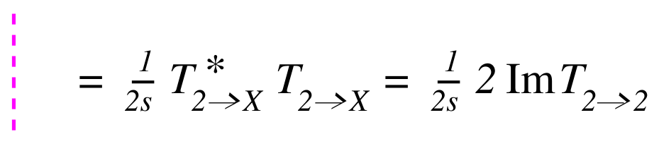
Figure 39: Conventions..

4.2 Elementary Interactions

Elementary nucleon-nucleon scattering can be considered as a straightforward generalization of photon-nucleon scattering: one has a hard parton-parton scattering in the middle, and parton evolutions in both directions towards the nucleons. We have a hard contribution $T_{\mathrm{hard}}$ when the the first partons on both sides are valence quarks, a semi-hard contribution $T_{\mathrm{semi}}$ when at least on one side there is a sea quark (being emitted from a soft Pomeron), and finally we have a soft contribution, when there is no hard scattering at all (see fig. 40). The total elementary elastic amplitude $T_{2\rightarrow 2}$ is the sum of all these terms.

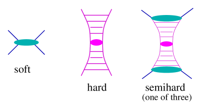
Figure 40: The elastic amplitude $T_{2\rightarrow 2}$.

We have a smooth transition from soft to hard physics: at low energies the soft contribution dominates, at high energies the hard and semi-hard ones, at intermediate energies (that is where experiments are performed presently) all contributions are important.

The multiple scattering theory will be based on these elementary interactions, the corresponding elastic amplitude $T_{2\rightarrow 2}$ and the corresponding cut diagram, both being represented graphically by a solid and a dashed vertical line. We also refer to the solid line as Pomeron, to the dashed line as cut Pomeron.

4.3 Multiple Scattering

We first consider inelastic proton-proton scattering, see fig. 41. We imagine an arbitrary number of elementary interactions to happen in parallel, where an interaction may be elastic or inelastic. The inelastic amplitude is the sum of all such contributions with at least one inelastic elementary interaction involved.

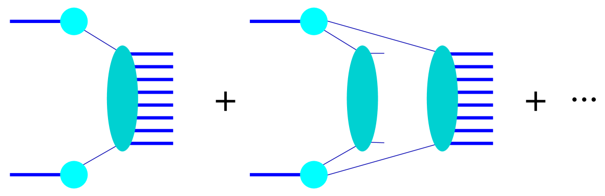
Figure 41: Inelastic scattering in pp.

To calculate cross sections, we need to square the amplitude, which leads to many interference terms, as the one shown in fig. 42(a), which represents interference between the first and the second diagram of fig. 41. Using the above notations, we may represent the left part of the diagram as a cut diagram, conveniently plotted as a dashed line, see fig. 42(b). The amplitude squared is now the sum over many such terms represented by solid and dashed lines.

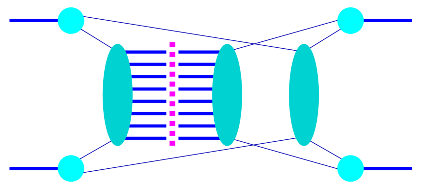
(a)       (b)

Figure 42: Inelastic scattering in pp. a) Amplitude, b) Squared amplitude makes

When squaring an amplitude being a sum of many terms, not all of the terms interfere – only those which correspond to the same final state. For example, a single inelastic interaction does not interfere with a double inelastic interaction, whereas all the contributions with exactly on inelastic interaction interfere. So considering a squared amplitude, one may group terms together representing the same final state. In our pictorial language, this means that all diagrams with one dashed line, representing the same final state, may be considered to form a class, characterized by $m=1$ – one dashed line ( one cut Pomeron) – and the light cone momenta $x^{+}$ and $x^{-}$ attached to the dashed line (defining energy and momentum of the Pomeron). In fig. 43, we show several diagrams belonging to this class, in fig. 44, we show the diagrams belonging to the class of two inelastic interactions, characterized by $m=2$ and four light-cone momenta $x_{1}^{+}$, $x_{1}^{-}$, $x_{2}^{+}$, $x_{2}^{-}$.

             

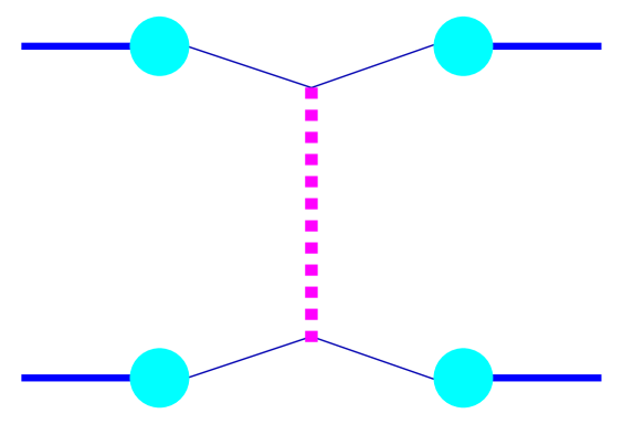
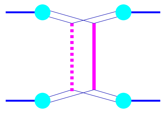
Figure 43: Class of terms corresponding to one inelastic interaction.

             

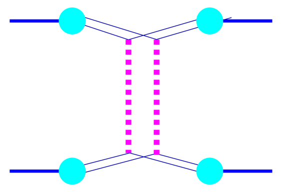
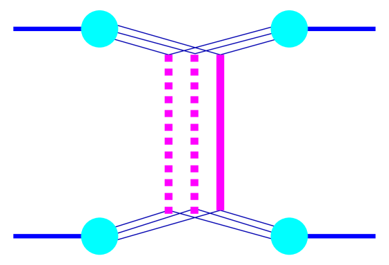
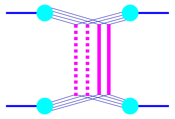
Figure 44: Class of terms corresponding to two inelastic interactions.

Generalizing these considerations, we may group all contributions with $m$ inelastic interactions ($m$ dashed lines = $m$ cut Pomerons) into a class characterized by the variable

$$K=\{m,x_{1}^{+},x_{1}^{-},\cdots,x_{m}^{+},x_{m}^{-}\}.$$

We then sum all the terms in a class $K$,

$$\Omega(K)=\sum\{\mathrm{all}\,\mathrm{terms}\,\mathrm{in}\,\mathrm{class}\,K\}.$$

The cross section is then simply a sum over classes,

$$\sigma_{\mathrm{inel}}(s)=\sum_{K\neq 0}\int d^{2}b\,\Omega(K).$$

$\Omega$ depends implicitly on the energy squared $s$ and the impact parameter $b$. The individual terms $\int d^{2}b\,\Omega(K)$, represent partial cross sections, since they represent distinct final states. They are referred to as topological cross sections.

The above concepts are easily generalized to nucleus-nucleus scattering, an example for a diagram representing a contribution to the squared amplitude is shown in fig. 45.

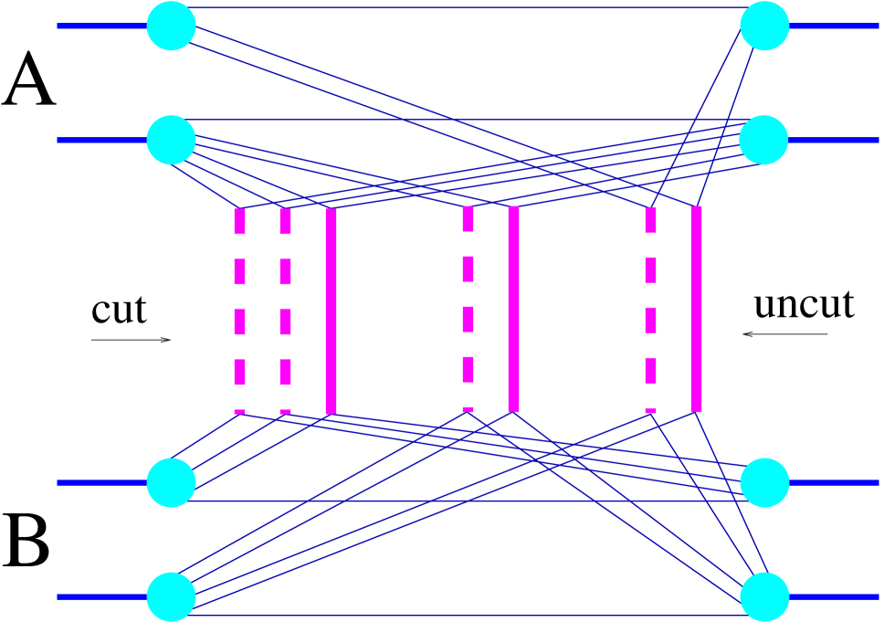
Figure 45: An interference term of total cross section of

We may also define classes, which correspond to well defined final states, in our notation a given number of dashed lines between nucleon pairs. We may number the pairs as 1, 2, 3, … $k$ … , $AB$. We define $m_{k}$ to be the number of inelastic interactions (cut Pomerons) of the pair number $k$. The $\mu^{\mathrm{th}}$ of these $m_{k}$ cut Pomerons is characterized by light cone momenta $x^{+}_{k\mu}$, $x^{-}_{k\mu}$. So a class may be characterized by

$$K=\{m_{k},x^{+}_{k\mu},x^{-}_{k\mu}\}.$$

We sum all terms in a class to obtain again a quantity called $\Omega(K),$ such that the cross section can be written as a sum over classes

$$\sigma_{\mathrm{inel}}(s)=\sum_{K\neq 0}\int d^{2}b\,\Omega(K),$$

as in the case of proton-proton scattering. Here, however, $b$ is a multidimensional variable representing the impact parameter $b_{0}$ and the transverse distances $b_{k}$ of all the nucleon-nucleon pairs. One can prove

$$\sum_{K}\Omega(K)=1,$$

which is a very important result justifying our interpretation of $\Omega(K)$ to be a probability distribution for the configurations $K$. This provides also the basis for applying Monte Carlo techniques.

The function $\Omega$ is the basis of all applications of this formalism. It provides the basis for calculating (topological) cross sections, but also for particle production, thus providing a consistent formalism for all aspects of a nuclear collision.

4.4 Pomeron-Pomeron Interactions

So far, we consider the case where particle production from the individual elementary interactions is completely independent. At high energies with high particle densities this is not very realistic: particles emitted in one interaction could be absorbed in another one. In our language: we have to allow interactions of Pomerons, like the diagrams shown in fig. 46.

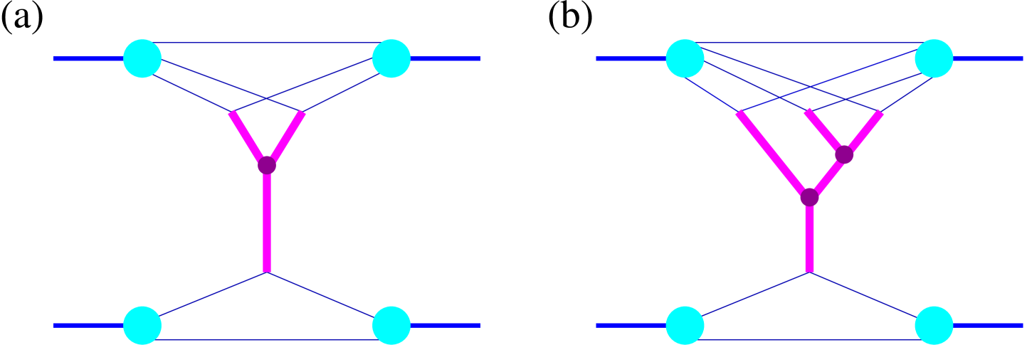
Figure 46: Pomeron-Pomeron interactions.

Such interactions are very important, being in particular responsible for screening (shadowing, saturation). If we assume for a moment that a Pomeron is roughly a parton ladder, then we we have the situation as shown in fig. 47: independent Pomerons correspond to non-interacting parton ladders (left figure), whereas Pomeron interaction amount to interactions of partons from one ladder with the ones from the other one (right figure). It is clear: the more partons are produced, the more likely are such processes.

      

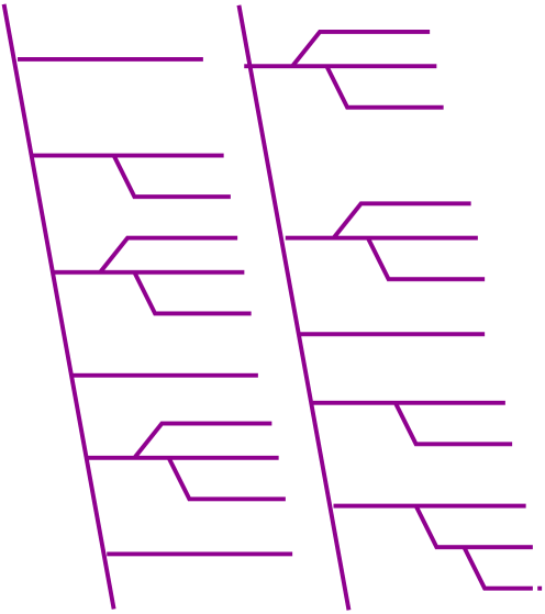
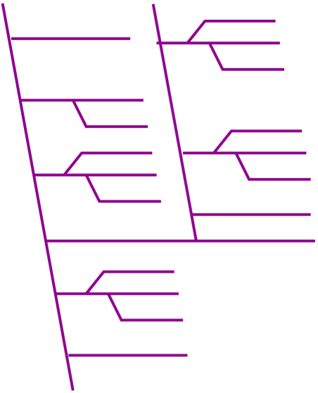
Figure 47: Pomeron-Pomeron interactions in parton language.

Also in case of Pomeron-Pomeron interactions, we are interested in particle production, and so we have to worry about cutting diagrams. Again, cut diagrams are the consequence of squaring amplitudes, i.e. multiplying an amplitude corresponding to some process with the complex conjugate amplitude corresponding to the same or some other process. In fig. 48, we show two examples: a ladder with an additional leg is multiplied with a simple ladder (left figure), and two ladders fused into one are multiplied with itself (right figure), We use again dashed and solid lines for cut and uncut diagrams.

      

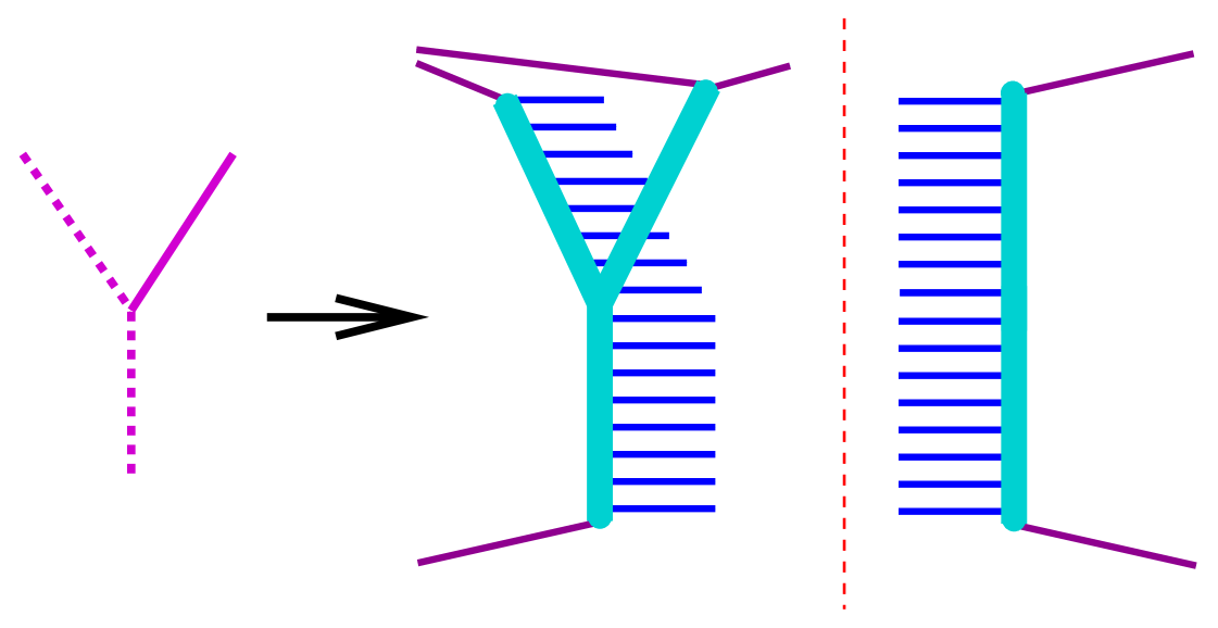
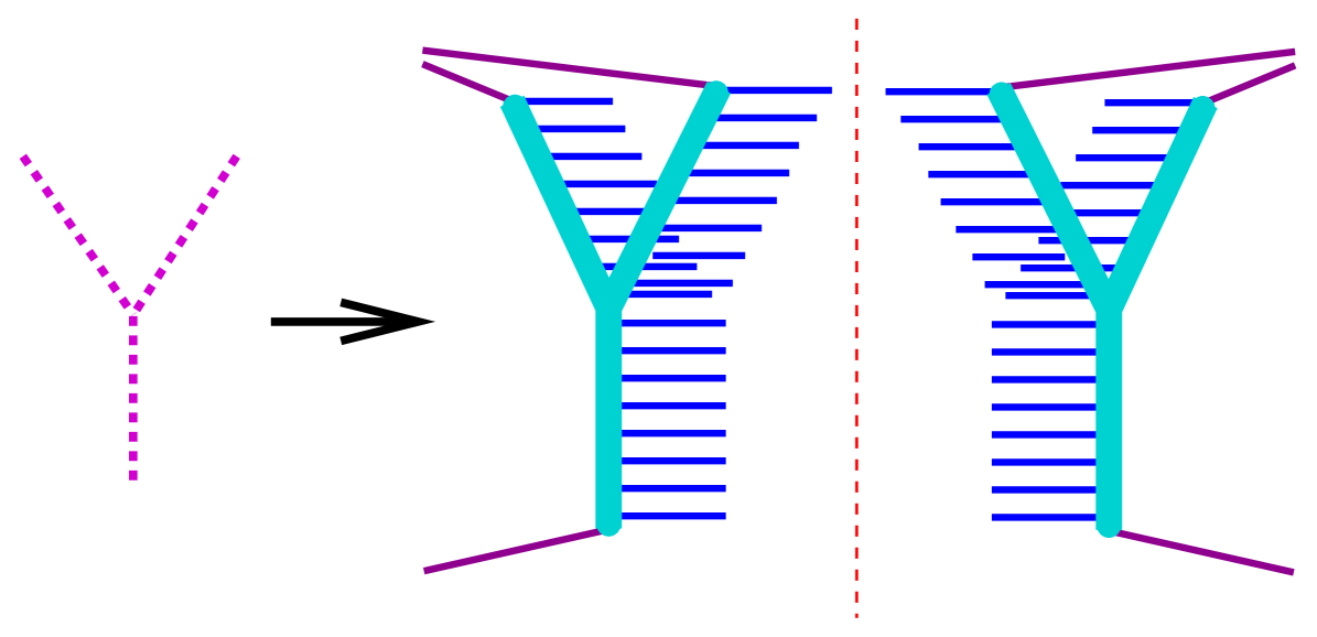
Figure 48: Cut diagrams as a result of squared amplitudes..

There are three cut diagrams of a Y diagram, as shown in fig. 49: the lower leg is always cut; in addition, there may be none (a) or one (b) or two (c) of the upper leg being cut.

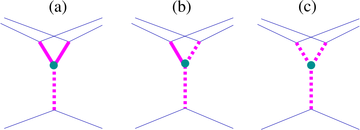
Figure 49: Cut Y diagrams.

An important property of this formalism is the so-called factorization. A dashed line corresponds to a cut Pomeron with given light cone momentum fractions $x^{+}$ and $x^{-}$. So the rapidity of the Pomeron is $1/2\,\mathrm{ln}\,\mathrm{x}^{+}/x^{-}$, the squared energy is $s\,x^{+}\,x^{-}$. Suppose this cut Pomeron represents a chain of particles with a typical transverse mass $m$. The range of rapidity is roughly given as $y^{-}<y<y^{+}$, with $y^{\pm}=\pm\ln(\sqrt{s}x^{\pm}/m)$ . So we may assign a vertical rapidity scale and draw the dashed vertical lines exactly between $y^{+}$ and $y^{-}$. In fig. 50, the diagrams have been plotted this way. The horizontal dashed line represents some given rapidity $y$. Due to some general rules, only those diagrams contribute to inclusive particle production at rapidity $y$, where exactly one line crosses the horizontal one. These are also the ones which factorize: they may be considered as a single line between two “blobs $(f)$”, each blob being an infinite sum, providing thus a simple effective diagram. All the non-factorizable diagrams do not contribute to the inclusive cross sections.

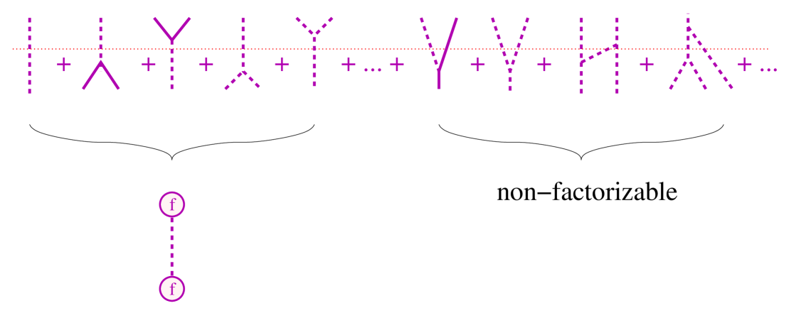
Figure 50: Factorization in $pp$ scattering.

In the same way, the structure function in deep inelastic scattering exhibits factorization, as shown in fig. 51, with the same blob $(f)$ as in $pp$ scattering.

51

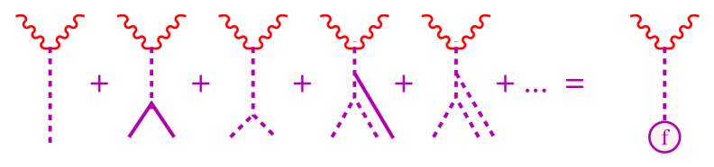
Figure 51: Factorization in deep inelastic scattering.

This allows to write the inclusive cross section in $pp$ as $f\times\hat{\sigma}\times f$, where $\hat{\sigma}$ represents the dashed line, and $f$ is obtained from deep inelastic scattering. Essentially we recover here the parton model.

Does this mean that one can hide all these complicated multiple scattering features in one simple measurable function $f$? The answer is yes if one is only interested in calculating inclusive spectra. However, the situation is completely different when it comes to the total cross section, where we have to consider all diagrams. The above-mentioned cancellations concern only inclusive cross sections. In addition, for Monte Carlo applications, we need to evaluate topological cross sections, related to the probabilities to certain configurations (defined by the numbers of cut Pomerons). Here again, no cancellations apply, we need to consider all diagrams.

In this sense, the so-called eikonal approach is very questionable, where total and topological cross sections are calculated based on inclusive ones, neglecting all the non-factorizable contributions.

References

- [1] H. J. Drescher, M. Hladik, S. Ostapchenko, T. Pierog, and K. Werner, Phys. Rept. 350, 93 (2001), hep-ph/0007198.
- [2] L. McLerran and R. Venugopalan, Phys. Rev. D49, 2233; 3352 (1994), hep-ph/9311205.
- [3] T. Sjostrand and M. van Zijl, Phys. Rev. D36, 2019 (1987).
- [4] X.-N. Wang, Phys. Rept. 280, 287 (1997), hep-ph/9605214.
- [5] A. B. Kaidalov and K. A. Ter-Martirosyan, Phys. Lett. 117B, 247 (1982).
- [6] A. Capella, U. Sukhatme, C.-I. Tan, and J. Tran Thanh Van, Phys. Rept. 236, 225 (1994).
- [7] P. Aurenche et al., Phys. Commun. 83, 107 (1994).
- [8] K. Werner, Phys. Rep. 232, 87 (1993).
- [9] K. Geiger and B. Muller, Nucl. Phys. B369, 600 (1992).
- [10] G. Baym, B. L. Friman, J. P. Blaizot, M. Soyeur, and W. Czyz, Nucl. Phys. A407, 541 (1983).
- [11] D. H. Rischke, (1998), nucl-th/9809044.
- [12] C. E. Aguiar, T. Kodama, T. Osada, and Y. Hama, (2000), hep-ph/0006239.
- [13] P. Rehberg, L. Bot, and J. Aichelin, Nucl. Phys. A653, 415 (1999), hep-ph/9809565.
- [14] M. Hofmann et al., Phys. Lett. B478, 161 (2000), nucl-th/9908030.
- [15] P. Csizmadia and P. Levai, In *Trento 1999, Understanding deconfinement in QCD* 324- 330.
- [16] S. A. Bass et al., Prog. Part. Nucl. Phys. 41, 225 (1998), nucl-th/9803035.
- [17] M. Bleicher et al., J. Phys. G25, 1859 (1999), hep-ph/9909407.
- [18] B.-A. Li and C. M. Ko, Phys. Rev. C52, 2037 (1995), nucl-th/9505016.
- [19] Y. Nara, Nucl. Phys. A638, 555C (1998), nucl-th/9802016.
- [20] TASSO, M. Althoff et al., Z. Phys. C22, 307 (1984).
- [21] ALEPH, R. Barate et al., Phys. Rep. 294, 1 (1998).
- [22] OPAL, G. Alexander et al., Z. Phys. C72, 191 (1996).
- [23] OPAL, K. Ackerstaff et al., Z. Phys. C75, 193 (1997).