Abstract

We compute the ${\cal O}(\alpha_{b}\alpha_{s})$ two–loop corrections to the neutral Higgs boson masses in the Minimal Supersymmetric Standard Model, using the effective potential approach. Such corrections can be important in the region of parameter space corresponding to $\tan\beta\gg 1$ and sizeable $\mu$. In spite of the formal analogy with the ${\cal O}(\alpha_{t}\alpha_{s})$ corrections, there are important differences, since the dominant effects are controlled by the sbottom–Higgs scalar couplings. We propose a convenient renormalization scheme that avoids unphysically large threshold effects associated with the bottom mass, and absorbs the bulk of the ${\cal O}(\alpha_{b}\alpha_{s}+\alpha_{b}\alpha_{t})$ corrections into the one–loop expression. We give general explicit formulae for the ${\cal O}(\alpha_{b}\alpha_{s})$ corrections to the neutral Higgs boson mass matrix. We also discuss the importance of the ${\cal O}(\alpha_{b}^{2})$ corrections and derive a formula for their contribution to $m_{h}$ in a simple limiting case.

1 Introduction

The existence of a light CP–even neutral Higgs boson is a crucial prediction of the Minimal Supersymmetric extension of the Standard Model, or MSSM, and has been one of the most active areas of theoretical investigations in the last decade. At the tree level, the masses of the neutral CP–even Higgs bosons of the MSSM can be computed in terms of three input parameters: the mass $m_{\scriptscriptstyle A}$ of the neutral CP–odd particle, the mass $m_{\scriptscriptstyle Z}$ of the weak neutral gauge boson, and the ratio of Higgs vacuum expectation values $\tan\beta\equiv v_{2}/v_{1}$ (for a review and references, see e.g. [1]). For $\tan\beta\ll m_{t}/m_{b}$, the dominant one–loop corrections are the ${\cal O}(\alpha_{t})$ ones, where $\alpha_{t}\equiv h_{t}^{2}/(4\pi)$ and $h_{t}$ is the superpotential top coupling. Such coupling controls both the top–Higgs Yukawa couplings and a number of cubic and quartic stop–Higgs scalar couplings, and leads to significant contributions from both top and stop loops [2]. The ${\cal O}(\alpha_{b})$ one–loop corrections associated with the superpotential bottom coupling $h_{b}$, where $\alpha_{b}\equiv h_{b}^{2}/(4\pi)$, can be numerically non–negligible only for $\tan\beta\gg 1$ and sizeable values of the $\mu$ parameter. At the classical level $h_{b}/h_{t}=(m_{b}/m_{t})\tan\beta$, thus we need $\tan\beta\gg 1$ to have $\alpha_{b}\sim\alpha_{t}$ in spite of $m_{b}\ll m_{t}$. Moreover, and in contrast with the top–stop case, numerically relevant contributions can only come from sbottom loops: those coming from bottom loops are always suppressed by the small value of the bottom mass. A sizeable value of $\mu$ is then required to have sizeable sbottom–Higgs scalar interactions in the large $\tan\beta$ limit.

We are now at the stage where the most important genuine two–loop corrections are being evaluated: general results have been obtained both for the ${\cal O}(\alpha_{t}\alpha_{s})$ [3, 4, 5] and for the ${\cal O}(\alpha_{t}^{2})$ [3, 6, 7] corrections. In this paper we move one step further, computing the ${\cal O}(\alpha_{b}\alpha_{s})$ corrections and discussing the ${\cal O}(\alpha_{b}^{2})$ and ${\cal O}(\alpha_{t}\alpha_{b})$ ones. For convenience, we evaluate two–loop effects directly in the physically relevant limit of large $\tan\beta$:

$$v_{1}\rightarrow 0\,,\;\;\;\;\;v_{2}\rightarrow v\equiv(\sqrt{2}\,G_{\mu})^{-1/2}\,,$$ (1)

where $G_{\mu}$ is the Fermi constant. As a result, we obtain extremely compact analytical formulae. Keeping $v_{1}\neq 0$ would only generate more complicated expressions, without adding any relevant information.

The plan of the paper is the following. We first give the analytical result at ${\cal O}(\alpha_{b}\alpha_{s})$ and in the $\overline{\rm DR}$ scheme. We then identify a convenient renormalization scheme that avoids unphysically large threshold effects and absorbs the largest ${\cal O}(\alpha_{b}\alpha_{s}+\alpha_{b}\alpha_{t})$ corrections into the one–loop expressions. In particular, we discuss how to use the experimental information on the bottom mass, which receives large threshold corrections [8], to extract the value of the renormalized coupling $h_{b}$. We finally present numerical results for some representative parameter choices, and conclude with an explicit formula for the ${\cal O}(\alpha_{b}\alpha_{s}+\alpha_{b}^{2})$ corrections to $m_{h}$ in a simple limiting case.

2 General formulae and $\overline{\rm DR}$ results

The momentum–independent part of the one–loop ${\cal O}(\alpha_{b})$ and two–loop ${\cal O}(\alpha_{b}\alpha_{s})$ corrections to the neutral CP–even Higgs boson mass matrix can be obtained by taking the second derivatives of the effective potential  at its minimum, or by performing appropriate substitutions and limits in the ${\cal O}(\alpha_{t}\alpha_{s})$ results of [5]. In the limit of Eq. (1), we find:

$$\left(\Delta{\cal M}^{2}_{S}\right)_{11}^{\rm eff} = \frac{1}{2}\,h_{b}^{2}\,s_{2\theta_{b}}^{2}\left[A_{b}^{2}\left(F^{\rm 1\ell}+F^{\rm 2\ell}\right)+2\,A_{b}\,m_{\tilde{g}}\,G^{\rm 2\ell}\right]\,,$$ (2)

$$\left(\Delta{\cal M}^{2}_{S}\right)_{12}^{\rm eff} = \frac{1}{2}\,h_{b}^{2}\,s_{2\theta_{b}}^{2}\left[\mu\,A_{b}\,\left(F^{\rm 1\ell}+F^{\rm 2\ell}\right)+\mu\,m_{\tilde{g}}\,G^{\rm 2\ell}\right]\,,$$ (3)

$$\left(\Delta{\cal M}^{2}_{S}\right)_{22}^{\rm eff} = \frac{1}{2}\,h_{b}^{2}\,s_{2\theta_{b}}^{2}\,\mu^{2}\,\left(F^{\rm 1\ell}+F^{\rm 2\ell}\right)\,.$$ (4)

Before explaining the meaning of the different symbols, we recall that an important simplification occurs if we look at the lightest Higgs eigenvalue, $m_{h}$, in the limit $m_{\scriptscriptstyle A}\gg m_{\scriptscriptstyle Z}$, since in that limit $\Delta m_{h}^{2}$ coincides with $(\Delta{\cal M}^{2}_{S})_{22}^{\rm eff}$. Our conventions are such that, at the classical level, the top and bottom quark masses are given by $m_{t}=h_{t}v_{2}/\sqrt{2}$ and $m_{b}=h_{b}v_{1}/\sqrt{2}$, where the Yukawa couplings $(h_{t},h_{b})$ and the VEVs $(v_{1},v_{2})$ are all taken to be real and positive. In addition, we assume $\mu$ and $A_{b}$ to be real, but we do not make any assumption on their sign, whereas we choose the gluino mass $m_{\tilde{g}}$ to be real and positive. At the classical level, the sbottom mixing angle $s_{2\theta_{b}}\equiv\sin 2\theta_{\tilde{b}}$ is given by

$$s_{2\theta_{b}}=\frac{\sqrt{2}\,h_{b}(A_{b}\,v_{1}+\mu\,v_{2})}{m_{\tilde{b}_{1}}^{2}-m_{\tilde{b}_{2}}^{2}}\longrightarrow\frac{\sqrt{2}\,h_{b}\,\mu\,v}{m_{\tilde{b}_{1}}^{2}-m_{\tilde{b}_{2}}^{2}}\,,$$ (5)

where the arrow denotes the large $\tan\beta$ limit, and $m_{\tilde{b}_{1}}^{2}>m_{\tilde{b}_{2}}^{2}$ are the two eigenvalues of the sbottom mass matrix. Finally, the superscripts in the functions $(F,\,G)$ indicate the order of the loop contribution. At one loop, and in the large $\tan\beta$ limit, the only relevant function is

$$F^{\rm 1\ell}=\frac{N_{c}}{16\,\pi^{2}}\left(2-\frac{m_{\tilde{b}_{1}}^{2}+m_{\tilde{b}_{2}}^{2}}{m_{\tilde{b}_{1}}^{2}-m_{\tilde{b}_{2}}^{2}}\,\ln\frac{m_{\tilde{b}_{1}}^{2}}{m_{\tilde{b}_{2}}^{2}}\right)\,,$$ (6)

where $N_{c}=3$ is a color factor. Notice that $F^{\rm 1\ell}$ is negative definite.

We first present our results for $F^{\rm 2\ell}$ and $G^{\rm 2\ell}$ in the $\overline{\rm DR}$ scheme. In other words, we assume that the ${\cal O}(\alpha_{b})$ one–loop contribution is written entirely in terms of $\overline{\rm DR}$ parameters (masses and couplings), evaluated at a certain renormalization scale $Q$. In units of $g_{s}^{2}\,C_{F}\,N_{c}/(16\,\pi^{2})^{2}$, where $C_{F}=4/3$, we find:

$$\hat{F}^{\rm 2\ell} = \left(2-\frac{m_{\tilde{b}_{1}}^{2}+m_{\tilde{b}_{2}}^{2}}{m_{\tilde{b}_{1}}^{2}-m_{\tilde{b}_{2}}^{2}}\,\ln\frac{m_{\tilde{b}_{1}}^{2}}{m_{\tilde{b}_{2}}^{2}}\right)\,\left(3+9\,c^{2}_{2\theta_{b}}\right)-\frac{3+13\,c_{2\theta_{b}}^{\,2}}{m_{\tilde{b}_{1}}^{2}-m_{\tilde{b}_{2}}^{2}}\,\left(m_{\tilde{b}_{1}}^{2}\,\ln\frac{m_{\tilde{b}_{1}}^{2}}{Q^{2}}-m_{\tilde{b}_{2}}^{2}\,\ln\frac{m_{\tilde{b}_{2}}^{2}}{Q^{2}}\right)$$ (7)

$$+\,3\,\frac{m_{\tilde{b}_{1}}^{2}+m_{\tilde{b}_{2}}^{2}}{m_{\tilde{b}_{1}}^{2}-m_{\tilde{b}_{2}}^{2}}\,\left(\ln^{2}\frac{m_{\tilde{b}_{1}}^{2}}{Q^{2}}-\ln^{2}\frac{m_{\tilde{b}_{2}}^{2}}{Q^{2}}\right)+4-c_{2\theta_{b}}^{\,2}\,\left[4-\left(\frac{m_{\tilde{b}_{1}}^{2}+m_{\tilde{b}_{2}}^{2}}{m_{\tilde{b}_{1}}^{2}-m_{\tilde{b}_{2}}^{2}}\right)^{2}\,\ln^{2}\frac{m_{\tilde{b}_{1}}^{2}}{m_{\tilde{b}_{2}}^{2}}\right.$$

$$\left.-6\,\frac{m_{\tilde{b}_{1}}^{2}+m_{\tilde{b}_{2}}^{2}}{(m_{\tilde{b}_{1}}^{2}-m_{\tilde{b}_{2}}^{2})^{2}}\,\left(m_{\tilde{b}_{1}}^{2}\,\ln\frac{m_{\tilde{b}_{1}}^{2}}{Q^{2}}-m_{\tilde{b}_{2}}^{2}\,\ln\frac{m_{\tilde{b}_{2}}^{2}}{Q^{2}}\right)\,\ln\frac{m_{\tilde{b}_{1}}^{2}}{m_{\tilde{b}_{2}}^{2}}\right]-\,s_{2\theta_{b}}^{2}\,\left[\frac{m_{\tilde{b}_{1}}^{2}}{m_{\tilde{b}_{2}}^{2}}+\frac{m_{\tilde{b}_{2}}^{2}}{m_{\tilde{b}_{1}}^{2}}\right.$$

$$\left.+2\,\ln\frac{m_{\tilde{b}_{1}}^{2}\,m_{\tilde{b}_{2}}^{2}}{Q^{4}}-\frac{m_{\tilde{b}_{1}}^{4}}{m_{\tilde{b}_{2}}^{2}\,(m_{\tilde{b}_{1}}^{2}-m_{\tilde{b}_{2}}^{2})}\,\ln\frac{m_{\tilde{b}_{1}}^{2}}{Q^{2}}+\frac{m_{\tilde{b}_{2}}^{4}}{m_{\tilde{b}_{1}}^{2}\,(m_{\tilde{b}_{1}}^{2}-m_{\tilde{b}_{2}}^{2})}\,\ln\frac{m_{\tilde{b}_{2}}^{2}}{Q^{2}}\,\right]$$

$$+\frac{4}{m_{\tilde{b}_{1}}^{2}-m_{\tilde{b}_{2}}^{2}}\left\{-\frac{m_{\tilde{b}_{2}}^{2}\,m_{\tilde{g}}^{2}}{m_{\tilde{b}_{1}}^{2}}+\frac{m_{\tilde{g}}^{2}m_{\tilde{b}_{2}}^{2}}{m_{\tilde{b}_{1}}^{2}}\,\ln\frac{m_{\tilde{g}}^{2}}{Q^{2}}-2\,m_{\tilde{g}}^{2}\,\ln\frac{m_{\tilde{b}_{1}}^{2}}{Q^{2}}\right.$$

$$\left.+\,\left(2\,m_{\tilde{g}}^{2}-m_{\tilde{b}_{1}}^{2}-m_{\tilde{b}_{2}}^{2}\right)\left[\,\ln\frac{m_{\tilde{g}}^{2}}{Q^{2}}\,\ln\frac{m_{\tilde{b}_{1}}^{2}}{Q^{2}}-{\rm Li}_{2}\left(1-\frac{m_{\tilde{b}_{1}}^{2}}{m_{\tilde{g}}^{2}}\right)\right]-\left(1\leftrightarrow 2\right)\;\right\}\,,$$

$$\hat{G}^{\rm 2\ell} = \frac{4}{m_{\tilde{b}_{1}}^{2}-m_{\tilde{b}_{2}}^{2}}\left[-4\,m_{\tilde{b}_{1}}^{2}+\left(3\,m_{\tilde{b}_{1}}^{2}+m_{\tilde{b}_{2}}^{2}\right)\,\ln\frac{m_{\tilde{b}_{1}}^{2}}{Q^{2}}-\,\left(m_{\tilde{b}_{1}}^{2}+m_{\tilde{b}_{2}}^{2}\right)\,\ln\frac{m_{\tilde{b}_{1}}^{2}}{Q^{2}}\ln\frac{m_{\tilde{g}}^{2}}{Q^{2}}\right.$$ (8)

$$\hskip 71.13188pt\left.-\left(2\,m_{\tilde{g}}^{2}-m_{\tilde{b}_{1}}^{2}-m_{\tilde{b}_{2}}^{2}\right)\,{\rm Li}_{2}\left(1-\frac{m_{\tilde{b}_{1}}^{2}}{m_{\tilde{g}}^{2}}\right)-\left(1\leftrightarrow 2\right)\right]\,,$$

where the hats on $F$ and $G$ denote ${\rm\overline{DR}}$–quantities, and, here and in the following, $(1\leftrightarrow 2)$ denotes the interchange $m_{\tilde{b}_{1}}^{2}\leftrightarrow m_{\tilde{b}_{2}}^{2}$. Notice that, in our limit, the bottom quark only contributes through bottom–sbottom–gluino diagrams. The above way of presenting the results is convenient for analysing models that predict, via the MSSM renormalization group equations, the low–energy $\overline{\rm DR}$ values of the MSSM input parameters in terms of a more restricted set of parameters, assigned as boundary conditions at some scale much larger than the weak scale. One of the parameters, however, is the $\overline{\rm DR}$ coupling $\hat{h}_{b}$, which must be connected with the experimental information on the bottom mass: this issue will be discussed extensively in Section 4.

3 A convenient renormalization prescription

General low–energy analyses of the MSSM parameter space do not refer to boundary conditions at high scales. These analyses are usually performed in terms of parameters with a more direct physical interpretation, such as pole masses and appropriately defined mixing angles in the squark sector. Such an approach requires modifications of our two–loop formulae, Eqs. (7)–(8), induced by the variation of the one–loop parameters when moving from the $\overline{\rm DR}$ scheme to a different scheme. We recall that, at the one–loop level, the two VEVs $(v_{1},v_{2})$ and the mass parameter $\mu$ are not renormalized by the strong interactions. Therefore, the only parameters in the Higgs mass matrix that require a one–loop definition are ($h_{b},\,A_{b},\,s_{2\theta_{b}},m_{\tilde{b}_{1}},\,m_{\tilde{b}_{2}}$), although only four of these are independent, because of the relation (5).

The sbottom masses $(m_{\tilde{b}_{1}}^{2},m_{\tilde{b}_{2}}^{2})$ in Eq. (6) can be naturally identified with the pole masses. For the generic parameter $x$, we define the shift from the $\overline{\rm DR}$ value $\hat{x}$ as $\delta x\equiv\hat{x}-x$. According to this definition, we find

$$\delta m_{\tilde{b}_{1}}^{2}\equiv\Pi_{11}(m_{\tilde{b}_{1}}^{2}) = \frac{g_{s}^{2}\,C_{F}}{16\pi^{2}}\,m_{\tilde{b}_{1}}^{2}\,\left[3\,\ln\frac{m_{\tilde{b}_{1}}^{2}}{Q^{2}}-3-c^{2}_{2\theta_{b}}\left(\ln\frac{m_{\tilde{b}_{1}}^{2}}{Q^{2}}-1\right)-s_{2\theta_{b}}^{2}\frac{m_{\tilde{b}_{2}}^{2}}{m_{\tilde{b}_{1}}^{2}}\left(\ln\frac{m_{\tilde{b}_{2}}^{2}}{Q^{2}}-1\right)\right.$$ (9)

$$\left.-6\frac{m_{\tilde{g}}^{2}}{m_{\tilde{b}_{1}}^{2}}-2\left(1-2\frac{m_{\tilde{g}}^{2}}{m_{\tilde{b}_{1}}^{2}}\right)\ln\frac{m_{\tilde{g}}^{2}}{Q^{2}}-2\left(1-\frac{m_{\tilde{g}}^{2}}{m_{\tilde{b}_{1}}^{2}}\right)^{2}\ln\left|1-\frac{m_{\tilde{b}_{1}}^{2}}{m_{\tilde{g}}^{2}}\right|\,\right]\,,$$

where $\Pi_{ij}(p^{2})$ denotes the real and finite part of the $(ij)$ component of the sbottom self–energy $(i,j=1,2)$, and $\delta m_{\tilde{b}_{2}}^{2}$ is obtained from Eq. (9) by the interchange $m_{\tilde{b}_{1}}^{2}\leftrightarrow m_{\tilde{b}_{2}}^{2}$.

The most convenient definition of $(h_{b},A_{b},s_{2\theta_{b}})$ is less easily singled out. To clarify this point, we recall the parallel case of the ${\cal O}(\alpha_{t}\alpha_{s})$ corrections. In that case, besides the stop pole masses, the remaining independent parameters are chosen to be [4, 5] a conveniently defined stop mixing angle, $s_{2\theta_{t}}$, and the top Yukawa coupling $h_{t}^{pole}$, as defined by the top pole mass $M_{t}$ via the relation $M_{t}\equiv h_{t}^{pole}v_{2}/\sqrt{2}$. Then, the stop counterpart of Eq. (5) is used to establish the one–loop definition of $A_{t}$ in terms of the pole top and stop masses and of the stop mixing angle. In the case of the ${\cal O}(\alpha_{b}\alpha_{s})$ corrections, a similar procedure is not appropriate since, as can be easily seen from Eq. (5), $s_{2\theta_{b}}$ is independent of $A_{b}$ in the large $\tan\beta$ limit. A second complication arises from the large one–loop threshold corrections [8] proportional to $v_{2}$ that contribute to the pole bottom mass: for our calculation, the relevant ones are those ${\cal O}(\alpha_{s})$, associated with one–loop SQCD diagrams with gluinos and sbottom quarks on the internal lines. As noticed in [9], a definition of $A_{b}$ in terms of the pole bottom and sbottom masses through Eq. (5) would produce very large shifts in $A_{b}$ with respect to its $\overline{\rm DR}$ value, $\delta A_{b}={\cal O}(\alpha_{s}\,\mu^{2}\,\tan^{2}\beta/m_{\tilde{g}})$. A $\overline{\rm DR}$ definition for the parameters $(h_{b},A_{b},s_{2\theta_{b}})$ would avoid this problem, but would still suffer from the known fact that it does not make manifest the decoupling of heavy particles, for example a heavy gluino.

We then look for definitions of the relevant parameters that automatically include the decoupling of heavy gluinos, allow to disentangle the genuine two–loop effects from the large threshold corrections to the bottom mass, and provide a consistent prescription for $A_{b}$ in the large $\tan\beta$ limit. There are two quantities that have a natural physical interpretation,

$$\widetilde{X}_{b}={h_{b}\,v\over\sqrt{2}}(c_{\beta}\,A_{b}+s_{\beta}\,\mu)\longrightarrow{h_{b}\,v\,\mu\over\sqrt{2}}\,,\;\;\;\;\;\widetilde{Y}_{b}={h_{b}\over\sqrt{2}}(s_{\beta}\,A_{b}-c_{\beta}\,\mu)\longrightarrow{h_{b}\,A_{b}\over\sqrt{2}}\,,$$ (10)

where the arrows denote as before the large $\tan\beta$ limit. At the classical level, $\widetilde{X}_{b}$ is the off–diagonal term in the sbottom mass matrix, related to the mixing angle $s_{2\theta_{b}}$ via Eq. (5), and $\widetilde{Y}_{b}$ is proportional to the coefficient of the trilinear $(\widetilde{b}_{L}\widetilde{b}_{R}^{*}A)$ interaction, or, equivalently, of the $(\widetilde{b}_{1}\widetilde{b}_{2}^{*}A)$ interaction.

A suitable definition of the mixing angle $\theta_{b}$, with the virtue of being infrared (IR) finite and gauge–independent with respect to the strong interaction, is [10]:

$$\delta\theta_{\tilde{b}}=\frac{1}{2}\,\frac{\Pi_{12}(m_{\tilde{b}_{1}}^{2})+\Pi_{12}(m_{\tilde{b}_{2}}^{2})}{m_{\tilde{b}_{1}}^{2}-m_{\tilde{b}_{2}}^{2}}\,,$$ (11)

where $\Pi_{12}(p^{2})$ turns out to be independent of $p^{2}$ in the large $\tan\beta$ limit. Using Eq. (5), the prescription on $\theta_{\tilde{b}}$ can be immediately translated into a prescription for $\widetilde{X}_{b}$:

$$\delta\widetilde{X}_{b}={1\over 2}\cos 2\theta_{b}\left[\Pi_{12}(m_{\tilde{b}_{1}}^{2})+\Pi_{12}(m_{\tilde{b}_{2}}^{2})\right]+\widetilde{X}_{b}\,\frac{\Pi_{11}(m_{\tilde{b}_{1}}^{2})-\Pi_{22}(m_{\tilde{b}_{2}}^{2})}{m_{\tilde{b}_{1}}^{2}-m_{\tilde{b}_{2}}^{2}}\,.$$ (12)

Since, in the large $\tan\beta$ limit, $v$ and $\mu$ are not renormalized by the strong interactions, the prescription on $\widetilde{X}_{b}$ can in turn be translated into a prescription for $h_{b}$. Explicitly:

$$\delta h_{b} = \frac{g_{s}^{2}\,C_{F}}{16\pi^{2}}\,h_{b}\,\left\{-4+2\,\ln\frac{m_{\tilde{g}}^{2}}{Q^{2}}\phantom{\left(\left(1-\frac{m_{\tilde{g}}^{2}}{m_{\tilde{b}_{1}}^{2}}\right)^{2}\ln\left|1-\frac{m_{\tilde{b}_{1}}^{2}}{m_{\tilde{g}}^{2}}\right|\right)}\right.$$ (13)

$$\left.+\left[\frac{2\,m_{\tilde{b}_{1}}^{2}}{m_{\tilde{b}_{1}}^{2}-m_{\tilde{b}_{2}}^{2}}\,\left(2\,\ln\frac{m_{\tilde{b}_{1}}^{2}}{m_{\tilde{g}}^{2}}-\left(1-\frac{m_{\tilde{g}}^{2}}{m_{\tilde{b}_{1}}^{2}}\right)^{2}\ln\left|1-\frac{m_{\tilde{b}_{1}}^{2}}{m_{\tilde{g}}^{2}}\right|\right)+\left(1\leftrightarrow 2\right)\right]\right\}\;.$$

We stress that our renormalized $h_{b}$, as defined above, differs at the one–loop level both from the $\overline{\rm DR}$ quantity $\hat{h}_{b}$ and from the quantity $h_{b}^{pole}$ that would be obtained by plugging the pole bottom mass, $M_{b}$, into the tree–level formula:

$$h_{b}\neq h_{b}^{pole}\equiv{M_{b}\sqrt{2}\over v_{1}}\;.$$ (14)

Concerning the definition of $A_{b}$, we observe that the Yukawa coupling $h_{b}$ multiplying $A_{b}$ can be absorbed in a redefinition of the trilinear soft–breaking term, $\widetilde{A}_{b}\equiv h_{b}A_{b}$. The shift in $\widetilde{A}_{b}$ could be defined via a physical process, e.g. one of the decays $\widetilde{b}_{1}\rightarrow\widetilde{b}_{2}\,A$ or $A\rightarrow\widetilde{b}_{1}\,\widetilde{b}_{2}^{*}$, but such a definition would suffer from the problem of infrared (IR) singularities associated with gluon radiation. To overcome this problem, and given our ignorance of the MSSM spectrum, we find less restrictive to define $\delta\widetilde{A}_{b}$ in terms of the $(\widetilde{b}_{1}\widetilde{b}_{2}^{*}A)$ proper vertex, at appropriately chosen external momenta and including suitable wave function corrections, so that the resulting combination is IR finite and gauge–independent, and gives rise to an acceptable heavy gluino limit. Denoting the proper vertex $\tilde{b}_{1}\tilde{b}_{2}^{*}A$ with $i\Lambda_{12A}(p_{1}^{2},p_{2}^{2},p_{A}^{2})$, we define :

$$\delta\widetilde{A}_{b} = -{i\over\sqrt{2}}\left[\Lambda_{12A}(m_{\tilde{b}_{1}}^{2},m_{\tilde{b}_{1}}^{2},0)+\Lambda_{12A}(m_{\tilde{b}_{2}}^{2},m_{\tilde{b}_{2}}^{2},0)\right]$$ (15)

$$+{1\over 2}\,\widetilde{A}_{b}\,\frac{\Pi_{11}(m_{\tilde{b}_{1}}^{2})+\Pi_{22}(m_{\tilde{b}_{1}}^{2})-\Pi_{11}(m_{\tilde{b}_{2}}^{2})-\Pi_{22}(m_{\tilde{b}_{2}}^{2})}{m_{\tilde{b}_{1}}^{2}-m_{\tilde{b}_{2}}^{2}}~{}.$$

The above definition can be interpreted as the large $\tan\beta$ limit of a renormalization prescription on $\widetilde{Y}_{b}$, as defined in Eq. (10), since in that limit $\widetilde{Y}_{b}\rightarrow\widetilde{A}_{b}/\sqrt{2}$. Notice the strong resemblance with the corresponding renormalization prescription on $\widetilde{X}_{b}$, Eq. (12). At ${\cal O}(\alpha_{s})$, gauge independence and IR finiteness follow from the fact that one–loop gluon diagrams satisfy the identity

$$\left[\Lambda_{12A}(p^{2},p^{2},0)\right]_{g}={i\widetilde{A}_{b}\over\sqrt{2}}\frac{\left[\Pi_{11}(p^{2})-\Pi_{22}(p^{2})\right]_{g}}{m_{\tilde{b}_{1}}^{2}-m_{\tilde{b}_{2}}^{2}}\,,$$ (16)

so that the gluon contribution to $\delta\widetilde{A}_{b}$ can be written simply as

$$[\delta\widetilde{A}_{b}]_{g}=\widetilde{A}_{b}\frac{\left[\Pi_{11}(m_{\tilde{b}_{1}}^{2})-\Pi_{22}(m_{\tilde{b}_{2}}^{2})\right]_{g}}{m_{\tilde{b}_{1}}^{2}-m_{\tilde{b}_{2}}^{2}}\,,$$ (17)

where the on–shell self–energies $\Pi_{11}(m_{\tilde{b}_{1}}^{2})$ and $\Pi_{22}(m_{\tilde{b}_{2}}^{2})$ are indeed gauge–independent and IR finite. Writing

$$\delta\widetilde{A}_{b}=\delta h_{b}\,A_{b}+h_{b}\,\delta A_{b}\,,$$ (18)

we find

$$\delta A_{b}=\frac{g_{s}^{2}\,C_{F}}{8\pi^{2}}\,m_{\tilde{g}}\left\{4-2\,\ln\frac{m_{\tilde{g}}^{2}}{Q^{2}}-\left[\left(1-\frac{m_{\tilde{g}}^{2}}{m_{\tilde{b}_{1}}^{2}}\right)\,\ln\left|1-\frac{m_{\tilde{b}_{1}}^{2}}{m_{\tilde{g}}^{2}}\right|+\left(1\leftrightarrow 2\right)\right]\right\}\,.$$ (19)

With our one–loop specifications of $h_{b}$ and $A_{b}$, Eqs. (13) and (19), the CP–even Higgs boson mass matrix takes again the form of Eqs. (2)–(4), but the one–loop part of the corrections must now be evaluated in our renormalization scheme, and the functions $F^{\rm 2\ell}$ and $G^{\rm 2\ell}$ read now, in units of $g_{s}^{2}\,C_{F}\,N_{c}/(16\,\pi^{2})^{2}$:

$$F^{\rm 2\ell} = -(1+s_{2\theta_{b}}^{2})\left(2-\frac{m_{\tilde{b}_{1}}^{2}+m_{\tilde{b}_{2}}^{2}}{m_{\tilde{b}_{1}}^{2}-m_{\tilde{b}_{2}}^{2}}\,\ln\frac{m_{\tilde{b}_{1}}^{2}}{m_{\tilde{b}_{2}}^{2}}\right)^{2}-\left(\ln\frac{m_{\tilde{b}_{1}}^{2}}{m_{\tilde{b}_{2}}^{2}}\right)^{2}$$

$$+ 4-2\left({m_{\tilde{g}}^{2}\over m_{\tilde{b}_{1}}^{2}}+{m_{\tilde{g}}^{2}\over m_{\tilde{b}_{2}}^{2}}\right)+4\left(\ln{m_{\tilde{b}_{1}}^{2}\over m_{\tilde{g}}^{2}}+\ln{m_{\tilde{b}_{2}}^{2}\over m_{\tilde{g}}^{2}}\right)$$

$$+ 4\frac{m_{\tilde{b}_{1}}^{2}+m_{\tilde{b}_{2}}^{2}-2\,m_{\tilde{g}}^{2}}{m_{\tilde{b}_{1}}^{2}-m_{\tilde{b}_{2}}^{2}}\left[{\rm Li}_{2}\left(1-\frac{m_{\tilde{b}_{1}}^{2}}{m_{\tilde{g}}^{2}}\right)-{\rm Li}_{2}\left(1-\frac{m_{\tilde{b}_{2}}^{2}}{m_{\tilde{g}}^{2}}\right)-{1\over 2}\ln\frac{m_{\tilde{b}_{1}}^{2}}{m_{\tilde{b}_{2}}^{2}}\right]$$

$$- \!2\left[\left(1+\frac{2\,m_{\tilde{b}_{1}}^{2}}{m_{\tilde{b}_{1}}^{2}-m_{\tilde{b}_{2}}^{2}}-\frac{2\,m_{\tilde{b}_{1}}^{4}}{(m_{\tilde{b}_{1}}^{2}-m_{\tilde{b}_{2}}^{2})^{2}}\ln\frac{m_{\tilde{b}_{1}}^{2}}{m_{\tilde{b}_{2}}^{2}}\right)\!\left(1-{m_{\tilde{g}}^{2}\over m_{\tilde{b}_{1}}^{2}}\right)^{2}\ln\left|1-{m_{\tilde{b}_{1}}^{2}\over m_{\tilde{g}}^{2}}\right|+\left(1\leftrightarrow 2\right)\right]\,,$$

$$G^{\rm 2\ell} = 4\,\ln{m_{\tilde{b}_{1}}^{2}m_{\tilde{b}_{2}}^{2}\over m_{\tilde{g}}^{4}}+4\,\frac{m_{\tilde{b}_{1}}^{2}+m_{\tilde{b}_{2}}^{2}-2\,m_{\tilde{g}}^{2}}{m_{\tilde{b}_{1}}^{2}-m_{\tilde{b}_{2}}^{2}}\left[{\rm Li}_{2}\left(1-\frac{m_{\tilde{b}_{1}}^{2}}{m_{\tilde{g}}^{2}}\right)-{\rm Li}_{2}\left(1-\frac{m_{\tilde{b}_{2}}^{2}}{m_{\tilde{g}}^{2}}\right)\right]$$ (21)

$$- \!\!\!2\,\left(2-\frac{m_{\tilde{b}_{1}}^{2}+m_{\tilde{b}_{2}}^{2}}{m_{\tilde{b}_{1}}^{2}-m_{\tilde{b}_{2}}^{2}}\,\ln\frac{m_{\tilde{b}_{1}}^{2}}{m_{\tilde{b}_{2}}^{2}}\right)\left[\left(1-{m_{\tilde{g}}^{2}\over m_{\tilde{b}_{1}}^{2}}\right)\ln\left|1-{m_{\tilde{b}_{1}}^{2}\over m_{\tilde{g}}^{2}}\right|+\left(1\leftrightarrow 2\right)\right]\,.$$

Notice that, in this scheme, $F^{\rm 2\ell}$ and $G^{\rm 2\ell}$ do not depend explicitly on $Q$. We also stress that, in terms of our renormalized quantities $(m_{\tilde{b}_{1}}^{2},m_{\tilde{b}_{2}}^{2},h_{b},A_{b})$, the corrections have a smooth heavy gluino limit. In fact, in contrast with the case of the ${\cal O}(\alpha_{t}\alpha_{s})$ corrections, the gluino decouples for $m_{\tilde{g}}\rightarrow\infty$, since $m_{\tilde{g}}\,G^{\rm 2\ell}\rightarrow 0$ and $F^{\rm 2\ell}$ reduces to the first line of Eq. (LABEL:G3bar).

4 Input parameters

Phenomenological analyses of the MSSM parameter space should exploit the experimental information on the bottom mass. Instead of expressing such information with the pole mass $M_{b}$, it is convenient to use directly the running mass, in the SM and in the $\overline{\rm DR}$ scheme, evaluated at the reference scale $Q_{0}=175$ GeV. Following a procedure outlined in [11], we take as input the SM bottom mass in the $\overline{\rm MS}$ scheme, $m_{b}(m_{b})^{\overline{\rm MS}}_{\rm SM}=4.23\pm 0.08$ GeV, as determined from the $\Upsilon$ masses [12]; we evolve it up to the scale $Q_{0}$ by means of suitable renormalization group equations [13]; finally, we convert it to the $\overline{\rm DR}$ scheme. The result, which accounts for the resummation of the universal large QCD logarithms, is:

$$\overline{m}_{b}\equiv m_{b}(Q_{0})_{\rm SM}^{\overline{\rm DR}}=2.74\pm 0.05\;{\rm GeV}\,.$$ (22)

The relation between $\hat{h}_{b}\equiv h_{b}(Q_{0})_{\rm MSSM}^{\overline{\rm DR}}$ and $\overline{m}_{b}$ of Eq. (22) is given by:

$$\hat{h}_{b}\equiv h_{b}(Q_{0})_{\rm MSSM}^{\overline{\rm DR}}={\overline{m}_{b}\sqrt{2}\over v_{1}}{1+\delta_{b}\over\left|1+\epsilon_{b}\right|}\,,$$ (23)

where

$$\delta_{b} = {\alpha_{s}\over 3\pi}\left\{{3\over 2}-\ln\frac{m_{\tilde{g}}^{2}}{Q_{0}^{2}}\phantom{\left(\frac{2\,m_{\tilde{g}}^{2}-m_{\tilde{b}_{1}}^{2}}{m_{\tilde{g}}^{2}-m_{\tilde{b}_{1}}^{2}}\right)}\right.$$ (24)

$$\left.+\frac{1}{2}\left[\frac{m_{\tilde{b}_{1}}^{2}}{m_{\tilde{g}}^{2}-m_{\tilde{b}_{1}}^{2}}\left(1-\left(\frac{2\,m_{\tilde{g}}^{2}-m_{\tilde{b}_{1}}^{2}}{m_{\tilde{g}}^{2}-m_{\tilde{b}_{1}}^{2}}-\frac{4\,m_{\tilde{g}}A_{b}}{m_{\tilde{b}_{1}}^{2}-m_{\tilde{b}_{2}}^{2}}\right)\ln\frac{m_{\tilde{g}}^{2}}{m_{\tilde{b}_{1}}^{2}}\right)+(1\leftrightarrow 2)\right]\right\}\,,$$

and

$$\epsilon_{b}\;=\;-{2\,\alpha_{s}\over 3\,\pi}\,\frac{m_{\tilde{g}}\,\mu\,\tan\beta}{m_{\tilde{b}_{1}}^{2}-m_{\tilde{b}_{2}}^{2}}\,\left[\frac{m_{\tilde{b}_{1}}^{2}}{m_{\tilde{b}_{1}}^{2}-m_{\tilde{g}}^{2}}\,\ln{m_{\tilde{b}_{1}}^{2}\over m_{\tilde{g}}^{2}}-\frac{m_{\tilde{b}_{2}}^{2}}{m_{\tilde{b}_{2}}^{2}-m_{\tilde{g}}^{2}}\,\ln{m_{\tilde{b}_{2}}^{2}\over m_{\tilde{g}}^{2}}\right]\,.$$ (25)

The running parameter $\hat{h}_{b}$ is the appropriate input quantity to be used with the $\overline{\rm DR}$ result presented in Section 2, while the formulae obtained in Section 3 should be used with $h_{b}=\hat{h}_{b}-\delta h_{b}$, as defined in that section, evaluating Eq. (13) for $Q=Q_{0}$.

Notice that in Eq. (23) the large ${\cal O}(\alpha_{s})$ threshold corrections [8] parametrized by $\epsilon_{b}$ have been resummed to all orders as in [14]. With the same strategy, we can easily include the ${\cal O}(\alpha_{t})$ threshold corrections to the bottom mass, which are expected to generate the largest two–loop ${\cal O}(\alpha_{t}\alpha_{b})$ corrections to the neutral Higgs boson masses. It is sufficient to add to $\epsilon_{b}$ the analogous quantity

$$\epsilon_{b}^{\,\prime}\;=\;-{\alpha_{t}\over 4\,\pi}\,\frac{A_{t}\,\mu\,\tan\beta}{m_{\tilde{t}_{1}}^{2}-m_{\tilde{t}_{2}}^{2}}\,\left[\frac{m_{\tilde{t}_{1}}^{2}}{m_{\tilde{t}_{1}}^{2}-\mu^{2}}\,\ln{m_{\tilde{t}_{1}}^{2}\over\mu^{2}}-\frac{m_{\tilde{t}_{2}}^{2}}{m_{\tilde{t}_{2}}^{2}-\mu^{2}}\,\ln{m_{\tilde{t}_{2}}^{2}\over\mu^{2}}\right]\,,$$ (26)

where the mixing between gauginos and higgsinos has been neglected, so that the masses of the higgsinos coincide with $\mu$.

For computing the two–loop ${\cal O}(\alpha_{t}\alpha_{s}+\alpha_{b}\alpha_{s})$ corrected Higgs masses, as will be done in the numerical examples of the next section, a suitable specification must be given for the parameters entering the tree-level mass matrix and the one–loop ${\cal O}(\alpha_{t}+\alpha_{b})$ corrections. In our effective potential approach, the tree-level mass matrix is expressed in terms of the pole mass $m_{\scriptscriptstyle A}$ and of the $\overline{\rm DR}$ parameter $\tan\beta$, evaluated at the reference scale $Q_{0}$, while the renormalization of the $Z$ boson mass (whose numerical value we fix at $m_{\scriptscriptstyle Z}=91.187$ GeV) does not affect the ${\cal O}(\alpha_{t}\alpha_{s}+\alpha_{b}\alpha_{s})$ corrections. The parameters $v=246.218$ GeV and $\mu$ first appear at the one–loop level and do not receive corrections at ${\cal O}(\alpha_{s})$. For the top–stop sector, we take as input the top pole mass, conventionally fixed at $M_{t}=175$ GeV, and the parameters $(m_{Q,\tilde{t}}\,,m_{U},A_{t})$ that can be derived by rotating the diagonal matrix of the On–Shell (OS) stop masses by the angle $\theta_{\tilde{t}}$, defined as in [5]. Concerning the sbottom sector, additional care is required, because of our non–trivial definition of $h_{b}$, Eq. (23), and of the fact that, at ${\cal O}(\alpha_{s})$, the parameter $m_{Q,\tilde{b}}$ entering the sbottom mass matrix differs from the corresponding stop parameter $m_{Q,\tilde{t}}$ by a finite shift [9]. We start by computing the renormalized coupling $h_{b}$ as given by Eqs. (22)–(25) and (13). Then we compute $m_{Q,\tilde{b}}$ following the prescription of [9]. Finally, we use the parameters $h_{b}$ and $m_{Q,\tilde{b}}$ to compute the actual values of the OS sbottom masses and mixing angle. The remaining input quantities, appearing only in the two–loop corrections, are the gluino mass $m_{\tilde{g}}$ and the strong coupling constant, whose numerical value we fix at $\alpha_{s}(Q_{0})=0.108$.

5 Numerical examples

We are now ready for some numerical examples. To prepare the ground, we study the variation of our renormalized $h_{b}$ with respect to other parameters, keeping the reference bottom mass $\overline{m}_{b}$ fixed to the central value of Eq. (22).

The left panel of Fig. 1 shows $h_{b}$ as a function of

Figure 1: The Yukawa coupling $h_{b}$, as defined in Eq. (23): as a function of $\mu$ for $\tan\beta=40$ (left panel); as a function of $\tan\beta$ for $\mu=1.2$ TeV (right panel). The other parameters are $A_{b}=2$ TeV, $m_{Q}=m_{D}=m_{\tilde{g}}=1$ TeV. The quantity $h_{b}^{pole}\equiv\sqrt{2}\,M_{b}/v_{1}$ is also shown for comparison.

$\mu$ (solid line), for $\tan\beta=40$. The other relevant parameters are chosen as $A_{b}=2$ TeV, $m_{Q}=m_{D}=m_{\tilde{g}}=1$ TeV (the precise definition of $m_{Q}$ is not relevant in this case). The quantity $h_{b}^{pole}=\sqrt{2}\,M_{b}/v_{1}$ is also shown as a dashed line. The curve corresponding to $\hat{h}_{b}$ would be very close to that of $h_{b}$, thus we do not display it. We see that having large values of $\tan\beta$ and $\mu$ is a necessary but not sufficient condition for having a sizeable $h_{b}$: when the threshold contribution to the bottom mass dominates, $|\epsilon_{b}|\gg 1$, $h_{b}$ must decrease for increasing values of $|\mu|\tan\beta$. We also see that, when there is an almost complete destructive interference between the two contributions to the bottom mass, $\epsilon_{b}\simeq-1$, the correct value of the bottom mass cannot be reproduced by the one–loop formula for $h_{b}$ in the perturbative regime, and the corresponding set of MSSM parameters must be discarded. Finally, we can see that the renormalized $h_{b}$ can be large only for positive  values of $\mu$. We then focus our attention on the case in which $\mu$ is large and positive, so that $h_{b}$ and the corresponding corrections to the Higgs masses can be sizeable.

For completeness, we should mention (for recent discussions and references, see e.g. [15]) that models with $b$–$\tau$ Yukawa coupling unification at the GUT scale favour, in our conventions, a positive sign of $\mu\,m_{\tilde{g}}$, which leads to a negative $\epsilon_{b}$. For sufficiently small $|\mu|$, radiative B decays and the muon anomalous magnetic moment may favour a negative sign of $\mu\,M_{2}$, where $M_{2}$ is the $SU(2)$ gaugino mass, and a positive sign of $\mu\,A_{t}$. Similar but more model–dependent constraints can be extracted, with the help of additional assumptions on the soft supersymmetry–breaking terms, from the cosmological relic density. Finally, having $\mu$ and $\tan\beta$ simultaneously large may require a certain amount of fine–tuning [16].

The right panel of Fig. 1 shows $h_{b}$ as a function of $\tan\beta$, for $\mu=1.2$ TeV. Again, the curve for $\hat{h}_{b}$ would be practically indistinguishable and we do not show it. The other parameters are chosen as in the left panel, and the value of $h_{b}^{pole}$ is also shown. We can see that, for this choice of parameters (to be taken in the following as a representative one), values of $\tan\beta$ much larger than 40–50 would imply a value of $h_{b}$ beyond the perturbative regime. On the other hand, for low values of $\tan\beta$ the coupling $h_{b}$ is even smaller than $h_{b}^{pole}$, and the corresponding corrections to the Higgs masses are expected to be negligible. For this reason, in the numerical examples of the ${\cal O}(\alpha_{b}\alpha_{s})$ corrections we restrict ourselves to values of $\tan\beta$ between 25 and 45.

Figure 2: The mass $m_{h}$ as a function of $\tan\beta$, for $m_{\scriptscriptstyle A}=120$ GeV (left panel) or 1 TeV (right panel). The other parameters are $\mu=1.2$ TeV, $A_{t}=A_{b}=2$ TeV, $m_{Q,\tilde{t}}=m_{U}=m_{D}=m_{\tilde{g}}=1$ TeV. The meaning of the different curves is explained in the text.

Figure 3: The mass $m_{h}$ as a function of $\mu$, for $m_{\scriptscriptstyle A}=120$ GeV (left panel) or 1 TeV (right panel). The other parameters are $\tan\beta=30$, $A_{t}=A_{b}=2$ TeV, $m_{Q,\tilde{t}}=m_{U}=m_{D}=m_{\tilde{g}}=1$ TeV. The meaning of the different curves is explained in the text.

Figs. 2 and 3 show the light Higgs mass $m_{h}$ as a function of $\tan\beta$ for $\mu=1.2$ TeV, and as a function of $\mu$ for $\tan\beta=30$, respectively. In each figure, the left panel corresponds to $m_{\scriptscriptstyle A}=120$ GeV and the right panel to $m_{\scriptscriptstyle A}=1$ TeV . The other input parameters are chosen as $A_{t}=A_{b}=2$ TeV, $m_{Q,\tilde{t}}=m_{U}=m_{D}=m_{\tilde{g}}=1$ TeV. For this choice of parameters, $m_{Q,\tilde{b}}$ differs from $m_{Q,\tilde{t}}$ by less than 1%. The curves in Figs. 2 and  3 correspond to the one–loop corrected  $m_{h}$ at ${\cal O}(\alpha_{t})$ (long–dashed line) and at ${\cal O}(\alpha_{t}+\alpha_{b})$ (dot–dashed line), and to the two–loop corrected $m_{h}$ at ${\cal O}(\alpha_{t}\alpha_{s})$ (short–dashed line) and at ${\cal O}(\alpha_{t}\alpha_{s}+\alpha_{b}\alpha_{s})$ (solid line), respectively. We can see from Fig. 2 that, while the ${\cal O}(\alpha_{t})$ prediction for $m_{h}$ is practically independent of $\tan\beta$ for $\tan\beta>25$, the ${\cal O}(\alpha_{b})$ corrections lower $m_{h}$ considerably when $\tan\beta$ increases. Fig. 3 shows that a similar decrease in $m_{h}$ occurs when $\mu$ increases. Both effects are enhanced by the steep dependence of the renormalized coupling $h_{b}$ on $\tan\beta$ and $\mu$, depicted in Fig. 1. Comparing the solid and the short–dashed curves, we can see that the ‘genuine’ two–loop ${\cal O}(\alpha_{b}\alpha_{s})$ corrections to the Higgs mass, given by Eqs. (2)–(4) and (LABEL:G3bar)–(21), are usually a small fraction of the ${\cal O}(\alpha_{b})$ ones, but the former can still reach several GeV when the latter are very large. In particular, for small $m_{\scriptscriptstyle A}$ the ${\cal O}(\alpha_{b}\alpha_{s})$ corrections can be comparable in magnitude with the ${\cal O}(\alpha_{t}\alpha_{s})$ ones. We stress that the absence of very large two–loop effects from the sbottom sector is a consequence of our renormalization prescription, which allows to set apart the $\tan\beta$–enhanced corrections, resummed to all orders in the renormalized coupling $h_{b}$. If we were to adopt for the sbottom sector the same renormalization scheme that we use for the stop sector, the dependence on $\tan\beta$ of the one–loop corrected $m_{h}$ would be smoother, but very large corrections (growing as $\tan^{2}\beta$) would appear at two loops, questioning the validity of the perturbative expansion.

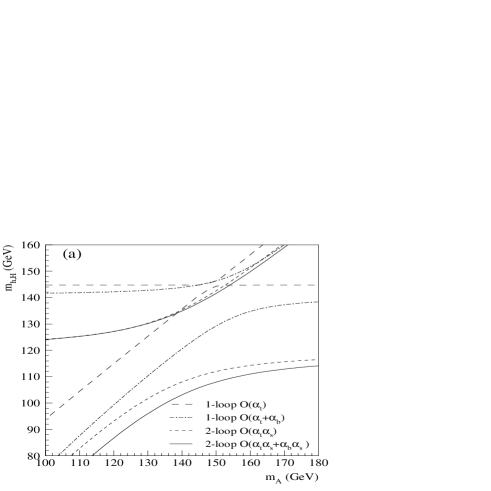
Figure 4: The masses $m_{h}$ and $m_{\scriptscriptstyle H}$ as a function of $m_{\scriptscriptstyle A}$, for $\mu=1.2$ TeV and $m_{Q,\tilde{t}}=m_{U}=m_{D}=m_{\tilde{g}}=1$ TeV. The other parameters are (a) $\tan\beta=40,\,A_{t}=A_{b}=2$ TeV and (b) $\tan\beta=45,\,A_{t}=1.5$ TeV, $A_{b}=0$. The meaning of the different curves is explained in the text.

Finally, Figs. 4a (left panel) and 4b (right panel) show both CP–even Higgs masses, $m_{h}$ and $m_{\scriptscriptstyle H}$, as functions of the CP–odd Higgs mass, in the region of relatively small $m_{\scriptscriptstyle A}$ (80 GeV $<m_{\scriptscriptstyle A}<$ 180 GeV), for two different choices of the parameters. In both figures we have chosen $\mu=1.2$ TeV and $m_{Q,\tilde{t}}=m_{U}=m_{D}=m_{\tilde{g}}=1$ TeV. In Fig. 4a the other parameters are $\tan\beta=40$ and $A_{t}=A_{b}=2$ TeV. From Fig. 4a we see that, as anticipated above, when $m_{\scriptscriptstyle A}$ is around 120 GeV the ${\cal O}(\alpha_{b}\alpha_{s})$ corrections to $m_{h}$ are of the same size of the ${\cal O}(\alpha_{t}\alpha_{s})$ ones. This is mainly due to the large value of $A_{b}$, which enhances the correction to $(\Delta{\cal M}^{2}_{S})_{11}^{\rm eff}$, relevant for $m_{h}$ when $m_{\scriptscriptstyle A}$ is small. The ${\cal O}(\alpha_{b}\alpha_{s})$ corrections to $m_{\scriptscriptstyle H}$ are rather small in this example, but they can be larger for different parameter choices. In Fig. 4b the relevant parameters are $\tan\beta=45\,,\,A_{t}=1.5$ TeV and $A_{b}=0$. For this choice, radiative corrections mainly affect $(\Delta{\cal M}^{2}_{S})_{22}^{\rm eff}$. Thus one of the eigenvalues is roughly degenerate with $m_{\scriptscriptstyle A}$ and receives small corrections, while the other eigenvalue is almost independent of $m_{\scriptscriptstyle A}$ and receives large corrections. In particular, the genuine ${\cal O}(\alpha_{b}\alpha_{s})$ corrections to either $m_{h}$ or $m_{\scriptscriptstyle H}$ are around 3 GeV in this example.

6 Conclusions and discussion

In this paper we presented explicit and general results for the ${\cal O}(\alpha_{b}\,\alpha_{s})$ corrections to the MSSM neutral Higgs boson masses, in the physically relevant limit of large $\tan\beta$. Actually, a large value of $\tan\beta$ is a necessary but not a sufficient condition for having large corrections, which require sizeable values of both $\mu$ and $h_{b}$. We proposed a renormalization prescription for the sbottom sector that automatically includes the decoupling of heavy gluinos and separates the large threshold corrections, appearing in the relation between $h_{b}$ and the pole bottom mass, from the genuine two–loop effects. We also discussed the numerical impact of our results in a number of representative examples.

A complete study of the two–loop (s)bottom corrections would require also the knowledge of the ${\cal O}(\alpha_{b}\alpha_{t})$ and ${\cal O}(\alpha_{b}^{2})$ effects. Concerning the former, it is plausible that the most important effects can be taken into account by adding to $\epsilon_{b}$ the analogous quantity $\epsilon_{b}^{\,\prime}$. The ${\cal O}(\alpha_{b}^{2})$ corrections would need a dedicated calculation, but an estimate of their importance can be obtained from our knowledge of the ${\cal O}(\alpha_{t}^{2})$ corrections. In Refs. [6, 7], explicit formulae for the ${\cal O}(\alpha_{t}^{2})$ corrections to the Higgs masses, valid under simplifying assumptions on the MSSM parameters, were presented. The corresponding formulae for the ${\cal O}(\alpha_{b}^{2})$ corrections can be derived from such formulae by performing suitable substitutions and taking appropriate limits. In the case of large $\tan\beta$ and universal soft sbottom masses, degenerate with $m_{\scriptscriptstyle A}$ and much larger than the weak scale $(m_{Q}=m_{D}=m_{\scriptscriptstyle A}\equiv M_{S}\gg v)$, it is possible to derive a simple expression for the ${\cal O}(\alpha_{b}+\alpha_{b}\,\alpha_{s}+\alpha_{b}^{2})$ corrections to $m_{h}^{2}$:

$$\Delta m_{h}^{2} \simeq -\frac{\widetilde{X}_{b}^{4}}{8\,\pi^{2}\,M_{S}^{4}\,v^{2}}\,\left\{1+\frac{4\,\alpha_{s}}{3\,\pi}\,f\left(\frac{m_{\tilde{g}}^{2}}{M_{S}^{2}}\right)+\frac{3\,\alpha_{b}}{4\,\pi}\,\left[\;f\left(\frac{\mu^{2}}{M_{S}^{2}}\right)-\frac{5}{2}\right.\right.$$ (27)

$$\left.\left.-\frac{\mu^{2}}{M_{S}^{2}}\,\left(2\,\ln\frac{|\widetilde{X}_{b}|}{M_{S}^{2}}+\frac{4}{3}\,\ln 2+1\right)+C\,\frac{A_{b}^{2}}{M_{S}^{2}}\right]\,\right\}\,,$$

where $\widetilde{X}_{b}=h_{b}\,v\,\mu/\sqrt{2}$ in the large $\tan\beta$ limit, $C\simeq 0.27$ and $f(x)$ is a positive function, defined as

$$f(x)\;=\;\frac{x\,(3\,x-2)}{x-1}-\frac{x^{2}\,(3\,x^{2}-8\,x+6)}{(x-1)^{2}}\,\ln x+(3\,x+1)\,(x-1)\,\ln|x-1|\;.$$ (28)

Some limiting values are $f(0)=0\,,\;f(1)=9/2,\>f(\infty)=3/2$. In view of the result in Eq. (27), we expect that, for values of $\alpha_{b}$ not much larger than $\alpha_{s}$, the ${\cal O}(\alpha_{b}^{2})$ corrections should be at most comparable with the ‘genuine’ ${\cal O}(\alpha_{b}\,\alpha_{s})$ effects.

References

[1]
J. F. Gunion, H. E. Haber, G. L. Kane and S. Dawson,
The Higgs Hunter’s Guide, Addison-Wesley, 1990
and (errata) hep-ph/9302272.
[2]
J. Ellis, G. Ridolfi and F. Zwirner,
Phys. Lett. B257 (1991) 83 and
Phys. Lett. B262 (1991) 477;
Y. Okada, M. Yamaguchi and T. Yanagida,
Prog. Theor. Phys. 85 (1991) 1 and
Phys. Lett. B262 (1991) 54;
H. E. Haber and R. Hempfling,
Phys. Rev. Lett. 66 (1991) 1815.
[3]
R. Hempfling and A. H. Hoang,
Phys. Lett. B331 (1994) 99 [hep-ph/9401219].
[4]
S. Heinemeyer, W. Hollik and G. Weiglein,
Phys. Rev. D58 (1998) 091701 [hep-ph/9803277],
Phys. Lett. B440 (1998) 296 [hep-ph/9807423],
Eur. Phys. J. C9 (1999) 343 [hep-ph/9812472],
and
Phys. Lett. B455 (1999) 179 [hep-ph/9903404];
R. Zhang, Phys. Lett. B447 (1999) 89 [hep-ph/9808299];
J. R. Espinosa and R. Zhang, JHEP 0003 (2000) 026 [hep-ph/9912236].
[5]
G. Degrassi, P. Slavich and F. Zwirner,
Nucl. Phys. B611 (2001) 403 [hep-ph/0105096].
[6]
J. R. Espinosa and R. Zhang,
Nucl. Phys. B586 (2000) 3 [hep-ph/0003246].
[7]
A. Brignole, G. Degrassi, P. Slavich and F. Zwirner,
Nucl. Phys. B631 (2002) 195 [hep-ph/0112177].
[8]
T. Banks, Nucl. Phys. B303 (1988) 172;
L. J. Hall, R. Rattazzi and U. Sarid,
Phys. Rev. D50 (1994) 7048 [hep-ph/9306309];
R. Hempfling, Phys. Rev. D49 (1994) 6168;
M. Carena, M. Olechowski, S. Pokorski and C. E. Wagner,
Nucl. Phys. B426 (1994) 269 [hep-ph/9402253].
[9]
A. Bartl, H. Eberl, K. Hidaka, T. Kon, W. Majerotto and Y. Yamada,
Phys. Lett. B402 (1997) 303 [hep-ph/9701398];
H. Eberl, K. Hidaka, S. Kraml, W. Majerotto and Y. Yamada,
Phys. Rev. D62 (2000) 055006 [hep-ph/9912463].
[10]
A. Pilaftsis,
Nucl. Phys. B504 (1997) 61 [hep-ph/9702393];
J. Guasch, J. Sola and W. Hollik, Phys. Lett. B437 (1998) 88
[hep-ph/9802329];
H. Eberl, S. Kraml and W. Majerotto, JHEP 9905 (1999) 016
[hep-ph/9903413];
Y. Yamada, Phys. Rev. D64 (2001) 036008 [hep-ph/0103046].
[11]
J. Ellis, T. Falk, G. Ganis, K. A. Olive and M. Srednicki,
Phys. Lett. B510 (2001) 236 [hep-ph/0102098].
[12]
M. Beneke and A. Signer, Phys. Lett. B471 (1999) 233 [hep-ph/9906475];
A. Hoang, Phys. Rev. D61 (2000) 034005 [hep-ph/9905550]
and hep-ph/0008102.
[13]
K. G. Chetyrkin, Phys. Lett. B404 (1997) 161 [hep-ph/9703278].
[14]
M. Carena, D. Garcia, U. Nierste and C. E. Wagner,
Nucl. Phys. B577 (2000) 88 [hep-ph/9912516];
G. Degrassi, P. Gambino and G. F. Giudice,
JHEP 0012 (2000) 009 [hep-ph/0009337].
[15]
U. Chattopadhyay, A. Corsetti and P. Nath, hep-ph/0204251;
H. Baer, C. Balazs, A. Belyaev, J. K. Mizukoshi, X. Tata and Y. Wang,
JHEP 0207 (2002) 050 [hep-ph/0205325].
[16]
A. E. Nelson and L. Randall,
Phys. Lett. B316 (1993) 516 [hep-ph/9308277].