Hypothetical first order $|\Delta S|=2$ transitions
in the $K^{0}-\overline{K^{0}}$ complex

Abstract

The influence of a hypothetical $CP$ violating $|\Delta S|=2$ interaction on the time evolution of the $K^{0}-\overline{K^{0}}$ system is investigated. It is shown, that if we were to assume the existence of the superweak-like interaction then this would lead to the conclusion, that there might be observable effects in the masses of the neutral kaons. We address the possibility of experimental observation of these effects and perform a computer simulation of one of the parameters which describe such effects. Instead of the widely used Lee, Oehme and Yang approximation which is not suitable to considering this kind of interaction we use a formalism based on the Królikowski-Rzewuski equation.

1 Introducton

Until recently there were two types of models of interactions which were considered plausible while investigating the source of the CP violation 1 . The miliweak models which assume that a part of order $10^{-3}G_{F}$ in the weak interaction was responsible for the observed CP violation effects. One of the most important predictions of this class of models is that the CP violation should be observed also in other than $K^{0}\rightleftarrows\overline{K^{0}}$ processes, and that it should be of the same order. The CKM model is an example of such miliweak models, at the same time being the most successful one. The recent experimental results concerning the measurement of $\frac{\epsilon^{\prime}}{\epsilon}$ and the $CP$ violation in the neutral $B$-meson system show, that the CKM model correctly describes the $CP$ violation. There is, however, a small possibility that a superweak-like interaction does exist, and some authors consider its implications (see 2 and references therein).

In the present paper we consider an effect which would be present, if the superweak interaction, or an interaction of a similar nature (the terms ’superweak’ and ’superweak-like’ will be used interchangeably), really existed in nature in addition to the CKM mechanism. We find, that the standard Weisskopf-Wigner approach to studying the $K^{0}\rightleftarrows\overline{K^{0}}$ process is not sensitive enough for the study of such an interaction, and therefore we choose the Krolikowski-Rzewuski approach 3 -4 and its extensions to the neutral kaon system suggested in 5 -8 . The paper is organized as follows. In the second section we review the most important (for our purposes) features of the Standard Model and the Superweak model and their present experimental status. The third section reviews the standard phenomenological approach to the neutral kaon system, which is based on the Weisskopf-Wigner approach. Also, basing on 9 , 5 -8 , we review an alternative formalism and analyze its relevance to the superweak-like interaction. The fourth section contains a computer simulation of the time dependence of one of the parameters introduced in the alternative model, namely the difference of the diagonal elements of the effective Hamiltonian, which in the presence of the superweak interaction turns out to be different from zero. The summary and conclusions are contained in the last section.

2 $K^{0}\rightleftarrows\overline{K^{0}}$ mixing in the Standard Model and the Superweak Model

In this section we quickly review the Standard Model approach to the $K^{0}\rightleftarrows\overline{K^{0}}$. We also briefly describe the salient features of the superweak scenario of $CP$ violation.

2.1 $K^{0}\rightleftarrows\overline{K^{0}}$ mixing and CP violation in the Standard Model

The flavour transitions allowed in the Standard Model are specified by the CKM matrix, which allows the following flavour mixing:

$$\left(\begin{array}[]{c}d^{\prime}\\ s^{\prime}\\ b^{\prime}\end{array}\right)=\left(\begin{array}[]{ccc}V_{ud}&V_{us}&V_{ub}\\ V_{cd}&V_{cs}&V_{cb}\\ V_{td}&V_{ts}&V_{tb}\\ \end{array}\right)\left(\begin{array}[]{c}d\\ s\\ b\end{array}\right).$$ (2.1)

Consequently, to the lowest order transitions $K^{0}\rightleftarrows\overline{K^{0}}$ can proceed through the diagrams presented in figure FIG. 1.

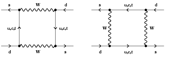
Figure 1: Diagrams corresponding to the $K^{0}\rightleftarrows\overline{K^{0}}$ process.

In the CKM theory there are no direct, first order $K^{0}\rightleftarrows\overline{K^{0}}$ transitions. In other words there are no first order $|\Delta S|=2$ transitions, or, in yet another equivalent formulation, which we will be using in the remaining part of the paper:

$$\langle{\bf 1}|H^{(1)}|{\bf 2}\rangle=0,$$ (2.2)

where $|K_{0}\rangle\equiv|{\bf 1}\rangle$ and $|{\overline{K}}_{0}\rangle\equiv|{\bf 2}\rangle$ and $H^{(1)}$ is the flavour-changing part of the weak Hamiltonian 10 .

Matrix 2.1 is unitary and contains $9$ parameters. Three of these parameters may be chosen to be real angles $\theta_{12}$, $\theta_{13}$, $\theta_{23}$ and the remaining six are phases. The number of phases can be reduced by using the fact, that spinors are defined up to a phase, so we may redefine the quark eigenstates. After doing this we notice, that in the procedure there are only five independent phase differences, whereas there are six phases in 2.1, so there is one physically meaningful phase in this unitary matrix. This is the crucial point of the $CKM$ theory because this phase allows for $CP$ violation 1 .

2.2 The hypothetical Superweak interaction

The Superweak model postulates the existence of a new $|\Delta S|=2$ interaction, which violates CP. The coupling constant of this interaction should be smaller than second order weak interaction. Thus, the superweak model assumes a non-vanishing first order transition matrix element:

$$\langle{\bf 1}|H^{(1)}|{\bf 2}\rangle\sim gG_{F}\neq 0,$$ (2.1)

where $g$ is the superweak coupling constant. It is widely accepted that this interaction can only be detected in the $K_{L}-K_{S}$, because it is the only known pair of states with the energy difference so small, that it is sensitive to interactions weaker than second order weak interaction 1 .

2.3 The status of the Standard Model and the Superweak model

The recent experimental results from the CPLEAR and KTeV Collaborations and others have given the decisive answer to the question whether the CP violation effects are correctly described by the $CKM$ miliweak theory. The measured value of $\frac{\epsilon^{\prime}}{\epsilon}=(1.72\pm 0.18)\times 10^{-3}$ 2 proves that there is a direct CP violating effect, and that CP violation cannot only be ascribed to mass mixing in the $K^{0}\rightleftarrows\overline{K^{0}}$ process. On the contrary: the CKM must be the dominant source of $CP$ violation (in low-energy flavour-changing processes)2 . Additionally, the measured value is perfectly consistent with the world average for the value $\frac{\epsilon^{\prime}}{\epsilon}$ 11 . Another experimental argument for the miliweak CKM theory are the two recent measurements of $CP$ violation in $B$ decays (2 and references therein). In other words, the Standard Model alone is able to correctly predict the value of $\frac{\epsilon^{\prime}}{\epsilon}$ and no improvements or extensions are in fact necessary.

However, even if the CP violation effects are described by the CKM the the idea of a $|\Delta S|=2$ interaction has not been abandoned entirely. Indeed, some authors consider the implications of such an interaction - the question of the existence of the superweak interaction turns out to be of some importance in the ”tagged” experiments in which the flavour is determined for the initial meson and then the for the meson at the time of decay. The existence of the $|\Delta S|=2$ superweak interaction might cause the production of the ”wrong” neutral meson states 12 . The effect of this hypothetical interaction is believed to be negligibly small as it would add to the $K^{0}\rightleftarrows\overline{K^{0}}$ mixing.

In the remaining part of the paper we want to discuss the implications of this hypothetical interaction for the time evolution of the $K^{0}-\overline{K^{0}}$ complex in the case of $CPT$ conservation in view of the recent experimental facts. We show that if we want to assume the existence of such an interaction then we can no longer use the LOY approximation. We also address the question of how this kind of interaction could have observable effects in the decay of the neutral mesons. The size of the effects introduced by the new, hypothetical interaction is also investigated, with the assumption that the recent experimental results and their interpretation are correct. To achieve this goal we will use a different approach than the LOY approximation, namely, a formalism based on the Królikowski-Rzewuski equation 3 , 4 .

3 The standard phenomenological description of the $K^{0}-\overline{K^{0}}$ system

In this section we briefly describe the phenomenology which is currently used to describe the time evolution of the $K^{0}-\overline{K^{0}}$ system.

3.1 The Lee, Oehme and Yang (LOY) approximation

This formalism is based on the formalism of particle mixture introduced by Gell-Mann and Pais 11a . The most important modification to this formalism was introduced by Lee, Oehme and Yang 10a , who, using the Weisskopf-Wigner approximation arrived at the formula (3.5) - see below - which is currently used. Further extensions were introduced by many other authors, e.g. Bell and Steinberger 12a .

In the standard approach the full Hamiltonian is divided into two parts:

$$H=H^{(0)}+H^{(1)},$$ (3.1)

where $H^{(0)}$ is the flavour-conserving part of the Hamiltonian, and $H^{(1)}$ is the flavour-changing part. The complete state vector which has evolved from ${\bf|1\rangle}$ or ${\bf|2\rangle}$ is projected onto the subspace spanned by ${\bf|1\rangle}$ and ${\bf|2\rangle}$. Therefore we define the state vector as:

$$|\Psi(t)\rangle=\alpha_{1}(t){\bf|1\rangle}+\alpha_{2}(t){\bf|2\rangle}.$$ (3.2)

Lee, Oehme and Yang, by modifying the Weisskopf-Wigner method for the single line, showed that the time dependence of the vector $\left(\begin{array}[]{c}\alpha(t)\\ \beta(t)\end{array}\right)$ can be described by the following Schrödinger-like equation:

$$i\frac{d}{dt}\left(\begin{array}[]{c}\alpha_{1}(t)\\ \alpha_{2}(t)\end{array}\right)=\left(\begin{array}[]{ll}H_{11}^{LOY}&H_{12}^{LOY}\\ H_{21}^{LOY}&H_{22}^{LOY}\end{array}\right)\left(\begin{array}[]{c}\alpha_{1}(t)\\ \alpha_{2}(t)\end{array}\right),$$ (3.3)

where we have adopted $\hbar=c=1$ and the matrix elements are matrix elements of the weak interaction transition operator. In the case of $CPT$ conserved it can be shown, that for this effective Hamiltonian we have $H_{11}^{LOY}=H_{22}^{LOY}$, but we have no information on $H_{12}^{LOY}$ or $H_{21}^{LOY}$ 10 .

The effective Hamiltonian can be split into two parts, each of them with a definite physical meaning, namely:

$$H^{LOY}=M-i\Gamma/2,$$ (3.4)

or

$$i\frac{d}{dt}\left(\begin{array}[]{c}\alpha_{1}(t)\\ \alpha_{2}(t)\end{array}\right)=\left(\begin{array}[]{cc}M-i\Gamma/2&M_{12}-i\Gamma_{12}/2\\ M_{21}-i\Gamma_{21}/2&M-i\Gamma/2\end{array}\right)\left(\begin{array}[]{c}\alpha_{1}(t)\\ \alpha_{2}(t)\end{array}\right).$$ (3.5)

The diagonal entries bear no indices, as we want to further emphasize the main result of the LOY approach, namely $H_{11}^{LOY}=H_{22}^{LOY}$.

For our purposes, which is the analysis of the influence of the hypothetical $|\Delta S|=2$ interaction on the time development of the $K^{0}-\overline{K^{0}}$ system, the LOY method is not suitable. Indeed, in 14 , 8 it was shown, that the LOY formulae may only be correct if we assume $\langle{\bf 1}|H^{(1)}|{\bf 2}\rangle=0$ and take $t\rightarrow\infty$. This obviously excludes the possibility of using the Lee, Oehme and Yang approximation in studying a hypothetical superweak interaction

3.2 The alternative approach

One alternative to the approach described above is the formalism developed in 5 —8 . We will briefly review this approximation and its basic findings.

The starting point of the derivation of an alternative effective Hamiltonian carried out in 8 ; 9 ; 14 is the Królikowski-Rzewuski Equation 3 ; 4 . In this approach the time evolution is not studied in the total space of states $\cal{H}$ but rather in a closed subspace $\cal{H}_{||}\subset\cal{H}$. If we define the following projector:

$$P\stackrel{{\scriptstyle\rm def}}{{=}}|\bf{1}\rangle\langle\bf{1}|+|\bf{2}\rangle\langle\bf{2}|,$$

then the subspace $\cal{H}_{||}$ may be defined as $\cal{H}_{||}=P{\cal H}$ or $|\psi;t\rangle_{||}=P|\psi;t\rangle$. In this way the total state space is split into two orthogonal subspaces $\cal{H}_{\parallel}$ and $\cal{H}_{\perp}=\cal{H}\ominus\cal{H}_{\parallel}$, and the Shrödinger equation can be replaced by equations describing each of the subspaces respectively. The equation for $\cal{H}_{\parallel}$ has the following form 3 ; 4 ; 9 :

$$\left(i\frac{\partial}{\partial t}-PHP\right)|\psi;t\rangle_{||}=|\chi;t\rangle-i\int_{0}^{\infty}K(t-\tau)|\psi;\tau\rangle_{||}d\tau,$$ (3.6)

$$Q=I-P,$$ (3.7)

$$K(t)=\Theta(t)PHQe^{-iQHQ}QHP,$$ (3.8)

$$|\chi;t\rangle=PHQe^{-iQHQ}|\psi\rangle_{\perp},$$ (3.9)

where

$$\Theta(t)=\left\{\begin{array}[]{lll}1&{\rm for}&t\geq 0\\ 0&{\rm for}&t<0\end{array}\right..$$

Following 3 ; 4 we introduce an effective Hamiltonian:

$$H_{||}(t)\equiv PHP+V_{||}(t).$$ (3.10)

This formula corresponds to (3.4), which also specifies an effective Hamiltonian.

Now, the main difference between the standard Lee, Oehme and Yang approximation and this approach is the effective potential. It can be shown that 8 ; 9 :

$$V_{||}(t)\simeq V_{||}^{1}(t)=-i\int_{0}^{\infty}K(t-\tau)e^{i(t-\tau)PHP}Pd\tau.$$ (3.11)

To establish notation let us now define the following symbols:

$$PHP\equiv\left[\begin{array}[]{ll}H_{11}&H_{12}\\ H_{21}&H_{22}\end{array}\right],$$ (3.12)

$$H_{ij}=\langle{\bf j}|H|{\bf i}\rangle\verb+ +,H_{0}\equiv\frac{1}{2}(H_{11}+H_{22}),\verb+ +\kappa\equiv\sqrt{|H_{12}|^{2}+\frac{1}{4}(H_{11}-H_{22})},\verb+ +H_{z}\equiv\frac{1}{2}(H_{11}-H_{22}).$$

The matrix elements $v_{ij}(t)=\langle{\bf j}|V_{||}(t)|{\bf i\rangle}$ of $V_{||}$ (3.11), without assuming any symmetries, like $[CP,H]=0$ or $[CPT,H]=0$ 8 ; 9 are:

$$v_{j1}(t)= - \frac{1}{2}\Big{(}1+\frac{H_{z}}{{\kappa}}\Big{)}{\Xi}_{j1}(H_{0}+{\kappa},t)$$

$$- \frac{1}{2}\Big{(}1-\frac{H_{z}}{{\kappa}}\Big{)}{\Xi}_{j1}(H_{0}-{\kappa},t)$$

$$- \frac{H_{21}}{2{\kappa}}{\Xi}_{j2}(H_{0}+{\kappa},t)+\frac{H_{21}}{2{\kappa}}{\Xi}_{j2}(H_{0}-{\kappa},t),$$

$$v_{j2}(t)= - \frac{1}{2}\Big{(}1-\frac{H_{z}}{{\kappa}}\Big{)}{\Xi}_{j2}(H_{0}+{\kappa},t)$$

$$- \frac{1}{2}\Big{(}1+\frac{H_{z}}{{\kappa}}\Big{)}{\Xi}_{j2}(H_{0}-{\kappa},t)$$

$$- \frac{H_{12}}{2{\kappa}}{\Xi}_{j1}(H_{0}+{\kappa},t)+\frac{H_{12}}{2{\kappa}}{\Xi}_{j1}(H_{0}-{\kappa},t),$$

where

$$\Xi(\lambda,t)\stackrel{{\scriptstyle\rm def}}{{=}}PHQ\frac{e^{-it(QHQ-\lambda)}-1}{QHQ-\lambda}QHP,$$ (3.15)

and ${\Xi}_{jk}(\varepsilon,t)=\langle{\bf j}\mid\Xi(\varepsilon,t)\mid{\it{\bf k}}\rangle$, and $j,k=1,2$. This effective potential, together with the remaining parts of the effective Hamiltonian yields the following matrix elements for the effective Hamiltonian:

$$h_{jk}(t)=\langle{\bf j}|H_{||}|{\bf k}\rangle=H_{jk}+v_{jk}(t),\;\;({\scriptstyle j,k=1,2}).$$ (3.16)

For the $[CPT,H]=0$ case the formulae simplify as $H_{z}=0$ in this case

Now, it is easy to notice that, in the case of $[CPT,H]=0$, contrary to the LOY effective Hamiltonian for which we have $H_{11}^{LOY}-H_{22}^{LOY}=0$ , the difference between the diagonal elements is non-vanishing:

$$h_{z}(t)=\frac{1}{2}(h_{11}(t)-h_{22}(t))\neq 0,(t>0).$$ (3.17)

It is also obvious that the necessary condition for (3.17) to be true is $H_{12}\neq 0$, that is, the existence a superweak interaction.

4 Computer simulation of the time evolution $h_{z}(t)$ within the Friedrichs-Lee model

In this section we perform a numerical simulation of the $h_{z}(t)$ parameter, which has proved so important in the present approach. By making some assumptions concerning the scale of the hypothetical superweak interaction we arrive at a form which is convenient for computer analysis. We also provide figures demonstrating the time evolution of the module and real and imaginary part of this parameter.

4.1 The Friedrichs-Lee model

In 8 the Friedrichs-Lee model was used to obtain the following formulae for the matrix elements of the effective Hamiltonian with the assumption $[CPT,H]=0$:

$$h_{j1}(t)=m_{j1}-\frac{1}{2}\left(\Gamma_{j1}+\frac{m_{21}}{|m_{12}|}\Gamma_{j2}\right)\Phi_{0}(t;m_{0}+|m_{12}|-\mu)-$$ (4.1)

$$-\frac{1}{2}\left(\Gamma_{j1}-\frac{m_{21}}{|m_{12}|}\Gamma_{j2}\right)\Phi_{0}(t;m_{0}-|m_{12}|-\mu),$$

$$h_{j2}(t)=m_{j2}-\frac{1}{2}\left(\Gamma_{j2}+\frac{m_{12}}{|m_{12}|}\Gamma_{j1}\right)\Phi_{0}(t;m_{0}+|m_{12}|-\mu)-$$ (4.2)

$$-\frac{1}{2}\left(\Gamma_{j2}-\frac{m_{12}}{|m_{12}|}\Gamma_{j1}\right)\Phi_{0}(t;m_{0}-|m_{12}|-\mu).$$

In these formulae $m_{0}\equiv\langle{\bf 1}|H^{(0)}|{\bf 1}\rangle=\langle{\bf 2}|H^{(0)}|{\bf 2}\rangle$, compare Eq.(3.1), $m_{12}\equiv H_{12}$; $m_{0}-\mu$ is the difference between the mass of the mesons considered and the threshold energy of the continuum state, like $K\rightarrow 2\pi$. Functions $\Phi_{0}(t,m)$ are defined by:

$$\Phi_{0}(t,m)=F_{0}(m)-F_{0}(t,m),$$ (4.3)

where

$$F_{0}(t,m)=\frac{a}{\sqrt{m}}[S(\sqrt{mt})-C(\sqrt{mt})]-$$ (4.4)

$$-i\frac{a}{\sqrt{m}}[C(\sqrt{mt})+S(\sqrt{mt})-1],$$

$$F_{0}(m)=i\frac{a}{\sqrt{m}},a=(m_{11}-\mu)^{\frac{1}{2}},$$ (4.5)

and finally $S(x)$ and $C(x)$ are the sine and cosine Fresnel integrals:

$$C(x)=\frac{1}{\sqrt{2}}\int_{0}^{x^{2}}\frac{\cos(\tau)}{\sqrt{\tau}}d\tau,$$

$$S(x)=\frac{1}{\sqrt{2}}\int_{0}^{x^{2}}\frac{\sin(\tau)}{\sqrt{\tau}}d\tau.$$

The parameters $\Gamma_{ij}$ correspond to the matrix elements of the decay matrix in the LOY approximation (3.5).

By setting $j=1$ in (4.1) and $j=2$ in (4.2) and then substracting (4.2) from (4.1)we get:

$$h_{z}(t)=\frac{m_{21}\Gamma_{12}-m_{12}\Gamma_{21}}{4|m_{12}|}[\Phi_{0}(t;m_{0}-|m_{12}|-\mu)-\Phi_{0}(t;m_{0}+|m_{12}|-\mu)].$$ (4.6)

Using a new independent variable $x$, defined in Appendix A we can rewrite $h_{z}(t)$ as:

$$h_{z}(x(t))=\frac{m_{21}\Gamma_{12}-m_{12}\Gamma_{21}}{4|m_{12}|}r(x),$$ (4.7)

where $r(x)$ has the following form (see Appendix A):

$$r(x)=\left(1-\frac{|m_{12}|}{m_{0}-\mu}\right)^{-\frac{1}{2}}\left\{i-\left[S\left(\sqrt{\left(1-\frac{|m_{12}|}{m_{0}-\mu}\right)x}\right)-C\left(\sqrt{\left(1-\frac{|m_{12}|}{m_{0}-\mu}\right)x}\right)\right]\right.$$ (4.8)

$$\left.-i\left[C\left(\sqrt{\left(1-\frac{|m_{12}|}{m_{0}-\mu}\right)x}\right)+S\left(\sqrt{\left(1-\frac{|m_{12}|}{m_{0}-\mu}\right)x}\right)\right]\right\}$$

$$+\left(1+\frac{|m_{12}|}{m_{0}-\mu}\right)^{-\frac{1}{2}}\left\{-i+\left[S\left(\sqrt{\left(1+\frac{|m_{12}|}{m_{0}-\mu}\right)x}\right)-C\left(\sqrt{\left(1+\frac{|m_{12}|}{m_{0}-\mu}\right)x}\right)\right]\right.$$

$$\left.-i\left[C\left(\sqrt{\left(1+\frac{|m_{12}|}{m_{0}-\mu}\right)x}\right)+S\left(\sqrt{\left(1+\frac{|m_{12}|}{m_{0}-\mu}\right)x}\right)\right]\right\}.$$

In spite of its complicated appearance, expression (4.8) is simple to analyze using computer methods as it contains no other variables but the independent variable $x$.

To extract any numerical information from (4.8) we need to make some assumptions concerning the strength of the superweak interaction. There are some estimates in the literature - we will accept the one suggested by Lee in 10 (equation 15.138, page 375): $\frac{|m_{12}|}{m_{0}-\mu}\simeq 10^{-17}$. To be sure, we do not even know if the strength is different from zero - we are assuming a value of $\frac{|m_{12}|}{m_{0}-\mu}$ which is consistent with the assumptions made in section 2. to see how $h_{z}(t)$ changes with time.

4.2 Time dependence of $h_{z}(x(t))$

Below we present three figures: the time dependence of $|r(x)|$, $\Re(r(x))$ and $\Im(r(x))$ - where $\Re$ and $\Im$ stand for the real and imaginary parts, respectively - which are proportional to the corresponding parameters connected with $h_{z}$, because from (1.13), (1.14) we have (see Appendix A):

$$|r(x)|=\frac{|h_{z}(x(t))|}{|\Gamma_{12}|\cdot|2\sin(\phi-\theta)|}.$$ (4.9)

The figures correspond to the value of $\frac{|m_{12}|}{m_{0}-\mu}$=$10^{-17}$.

Figure 2: The change of $y\sim|h_{z}(x)|$ in the logarithmic scale for the value $\frac{|m_{12}|}{m_{0}-\mu}=10^{-17}$.

Figure 3: The change of $y\sim\Re[h_{z}(x)]$ for long times in the logarithmic scale for $\frac{|m_{12}|}{m_{0}-\mu}=10^{-17}$.

Figure 4: The change of $y\sim\Im[h_{z}(t)]$ for long times in the logarithmic scale for $\frac{|m_{12}|}{m_{0}-\mu}=10^{-17}$.

In FIG. 2 we show the time dependence of the module of $r(x)$, which is basically the same as $|h_{z}(x)|$ This figure is in the logarithmic scale - we can see, that the parameter $r(x)$ oscillates around the constant value of around $10^{-16}$.The imaginary part rapidly tends to zero. Therefore the real part of $h_{z}(x)$ is responsible for the non-vanishing of $|h_{z}(x)|$ - this is clearly seen in FIG 3.

In the standard approach the real parts of the diagonal elements of the effective Hamiltonian are interpreted as the masses of the particles. Therefore it seems that the existence of the superweak interaction would remove the mass degeneracy between the particle and antiparticle in the neutral kaon system. Correspondingly, the imaginary parts are interpreted as the decay constants, so in the model considered the decay widths of the particle and antiparticle should be equal, which is consistent with the standard result. These results are consistent with the conclusions reached earlier on the basis of the form of $h_{z}(t)$ for large times - see Appendix B.

4.3 Order-of-magnitude estimation of the effect introduced by the superweak interaction

In this short subsection we try to estimate the order of magnitude of the effect introduced by the hypothetical superweak-like interaction. To this end we use the assumption, that the dominating contribution to $|\Gamma_{12}|$ is correctly described by the Standard Model. This means that we may assume

$$|\Gamma_{12}|\sim\frac{G^{2}_{F}M_{P}^{4}\sin^{2}\theta}{(2\pi)^{4}}m_{K_{0}}\sim 10^{-12}MeV,$$ (4.10)

where $G_{F}$ is the Fermi constant, $M_{P}$ is the proton mass and $\theta$ is the Cabbio angle 15 . Using our result form the previous section, $r(x\rightarrow\infty)\sim 10^{-16}$ and Equation 4.9 we get the following upper bound on our parameter:

$$\frac{|h_{z}(t\rightarrow\infty)|}{m_{K_{0}}}\lesssim\frac{1}{2}10^{-31}.$$ (4.11)

This value corresponds to the presently measured $|\frac{m_{K_{0}}-m_{\overline{K_{0}}}}{m_{K_{0}}}|\leq 10^{-18}$ 16 . Obviously, the effect calculated in the present paper is much too small to be observed with the present, and possibly also future, experiments. With this result, the question of the utility of the very concept of the superweak interaction arises.

5 Summary and Conclusions

In the present paper the influence of the hypothetical superweak interaction on the time evolution of the neutral kaon complex has been studied. We have investigated the dependence of the effective Hamiltonian on the very existence of such an interaction and found, that the standard Weisskopf-Wigner approach, used for example by Lee, Oehme and Yang 10 may only be correct if we assume the nonexistence of this interaction. This is the reason for choosing another approach, namely the formalism based on the Krolikowski-Rzewuski equation 5 -8 , which makes no such assumptions and is sensitive to the existence of the first order $|\Delta S|=2$ interaction. The two approaches have been shown to be equivalent in e.g. 14 in the absence of this interaction, but its inclusion leads to a prediction which is different from the generally accepted result.

The computer simulation of the time dependence of the parameter $|h_{z}(t)|$, corresponding to the difference of the diagonal elements of the effective Hamiltonian, presented in section 5. shows, that this parameter is different from zero and basically constant. Another result of this section is that it is the real part which is responsible for the non-vanishing $|h_{z}(t)|$, as the imaginary part very rapidly tends to zero. All these results would be impossible to reach without the Krolikowski-Rzewuski approach, further developed in 5 -8 , as the standard method due to Lee, Oehme and Yang is insensitive to the superweak interaction.

The prediction of the standard Lee-Oehme and Yang states that the real parts of the diagonal elements of the effective Hamiltonian governing the time evolution of the neutral kaon system should be equal. In the usual interpretation, the real parts of the diagonal elements correspond to the masses of the particles and hence the masses of $K^{0}$ and $\overline{K^{0}}$ are equal. In the approach assumed in the present paper the real parts of the effective halimtonian are equal on condition that there is no superweak interaction. The result of the present paper, and many others 5 -10 , 9 , 10 , is that mathematically the difference between the masses of particles and antiparticles needs not be equal to zero, if we assume the standard identification of the diagonal elements of the effective Hamiltonian plus the existence of the superweak-like interaction. However, even if this mathematical property of the effective Hamiltonian were to produce some results which are meaningful for the experiment, sensitivity of the instruments would have exceed the present day experiments by a few orders of magnitude (see section 4.3). Naturally, the question of the utility of the theory developed above should be raised. It is quite possible, that this formalism and the numerical results may only be used to confirm the standard result laid out in 10a .

Finally, it should be stressed that all the results obtained in the present paper are consistent with the Standard Model and the recent experimental findings. We have been assuming, that even if there is a CP violating $|\Delta S|=2$ interaction, the $K^{0}-\overline{K^{0}}$ complex is correctly described by the Standard Model to a high degree of accuracy. This is the reason for assuming $\frac{|m_{12}|}{m_{0}-\mu}=10^{-17}$ in section 5. and $|\Gamma_{12}|\sim 10^{-12}MeV$ in section 4.3.

*

Appendix A A

By rewriting the $m_{12}$ and $\Gamma_{12}$ parameters as:

$$m_{21}=m_{12}^{*}\equiv|m_{12}|e^{-i\theta},$$ (1.12)

$$\Gamma_{12}=\Gamma_{21}^{*}\equiv|\Gamma_{12}|e^{i\phi},$$

we may cast $h_{z}(t)$ in the following form:

$$h_{z}(t)=\frac{1}{4}|\Gamma_{12}|(e^{i(\phi-\theta)}-e^{-i(\phi-\theta)})\times$$ (1.13)

$$\times[\Phi_{0}(t;m_{0}-|m_{12}|-\mu)-\Phi_{0}(t;m_{0}+|m_{12}|-\mu)]=$$

$$=i|\Gamma_{12}|2\sin(\phi-\theta)[\Phi_{0}(t;m_{0}-|m_{12}|-\mu)-\Phi_{0}(t;m_{0}+|m_{12}|-\mu)].$$

It is easy to notice, that if $\phi=\theta$ we have $h_{z}=0$, but this case corresponds exactly to the $CP$ conserved case - compare 8 page 3743. Let us assume from now on, that we are dealing with the $CP$-violating, $CPT$-conserving case in which $\sin(\phi-\theta)\neq 0$.

To make our formulae simpler, let us define:

$$r(t)=[\Phi_{0}(t;m_{0}-|m_{12}|-\mu)-\Phi_{0}(t;m_{0}+|m_{12}|-\mu)].$$ (1.14)

So now

$$r(t)=F_{0}(m_{0}-|m_{12}|-\mu)-F_{0}(t;m_{0}-|m_{12}|-\mu)-$$ (1.15)

$$-F_{0}(m_{0}+|m_{12}|-\mu)+F_{0}(t;m_{0}+|m_{12}|-\mu).$$

Let us now transform the above expression using:

$$\sqrt{m_{0}-|m_{12}|-\mu}=\sqrt{m_{0}-\mu}\cdot\sqrt{1-\frac{|m_{12}|}{m_{0}-\mu}},$$

and

$$\sqrt{m_{0}+|m_{12}|-\mu}=\sqrt{m_{0}-\mu}\cdot\sqrt{1+\frac{|m_{12}|}{m_{0}-\mu}},$$

and a new, dimensionless variable

$$x\equiv(m_{0}-\mu)\cdot t.$$ (1.16)

If we define $\tau_{L}=5.2\cdot 10^{-8}s$ as the mean lifetime of $K_{L}$, the value of $x$ corresponding to this time is $x\simeq 2\cdot 10^{16}$.

Now we have:

$$(m_{0}-|m_{12}|-\mu)t=(m_{0}-\mu)(1-\frac{|m_{12}|}{m_{0}-\mu})t=(1-\frac{|m_{12}|}{m_{0}-\mu})x,$$ (1.17)

$$(m_{0}+|m_{12}|-\mu)t=(m_{0}-\mu)(1+\frac{|m_{12}|}{m_{0}-\mu})t=(1+\frac{|m_{12}|}{m_{0}-\mu})x.$$

Using the above and Equation (1.15) we arrive at (4.8).

Appendix B B

In 8 the following formula for the behaviour of $h_{z}(t)$ in the long time region was derived:

$$h_{z}(t)\simeq_{t\rightarrow\infty}\frac{m_{21}\Gamma_{12}-m_{12}\Gamma_{21}}{4|m_{12}|}\left\{F_{0}(m_{0}-|m_{12}|-\mu)-F_{0}(m_{0}-|m_{12}|-\mu)\right.$$ (2.18)

$$\frac{1+i}{\sqrt{2\pi}}\frac{a_{1}(0)}{\sqrt{t}}e^{-i(m_{0}-\mu)t}\left[\frac{e^{i|m_{12}|t}}{m_{0}-|m_{12}|-\mu}-\frac{e^{-i|m_{12}|t}}{m_{0}+|m_{12}|-\mu}\right]\left.\right\}.$$

Let us write out the real and imaginary parts of the above expression in terms of masses, $\Gamma_{ij}$ and $|m_{ij}|$:

$$\Re(h_{z}(t\rightarrow\infty))=-(m_{11}-\mu)^{\frac{1}{2}}\frac{\Im(m_{21}\Gamma_{12})}{2|m_{12}|}\left\{\frac{\sqrt{m_{0}-\mu+|m_{12}|}-\sqrt{m_{0}-\mu-|m_{12}|}}{\sqrt{(m_{0}-\mu)^{2}-|m_{12}|^{2}}}+\right.$$ (2.19)

$$+\frac{1}{\sqrt{2\pi}\sqrt{t}}\left[\frac{\sin(m_{0}-\mu-|m_{12}|)t-\cos(m_{0}-\mu-|m_{12}|)t}{m_{0}-\mu-|m_{12}|}\right.$$

$$\left.\left.-\frac{\sin(m_{0}-\mu+|m_{12}|)t-\cos(m_{0}-\mu+|m_{12}|)t}{m_{0}-\mu+|m_{12}|}\right]\right\},$$

$$\Im(h_{z}(t\rightarrow\infty))=-(m_{11}-\mu)^{\frac{1}{2}}\frac{1}{\sqrt{2\pi}\sqrt{t}}\frac{\Im(m_{21}\Gamma_{12})}{2|m_{12}|}\left\{\frac{\sin(m_{0}-\mu-|m_{12}|)t+\cos(m_{0}-\mu-|m_{12}|)t}{m_{0}-\mu-|m_{12}|}\right.$$

$$-\left.\frac{\sin(m_{0}-\mu+|m_{12}|)t+\cos(m_{0}-\mu+|m_{12}|)t}{m_{0}-\mu+|m_{12}|}\right\}.$$

From these formulae it is clear, that the imaginary part tends to zero and the real part tends to a constant.

References

• (1) K.Kleinknecht, $CP$ Violation in the $K^{0}-\overline{K}^{0}$ System in $CP$ Violation, Eds. C.Jarlskog, World Scientific, Singapore, (1989).
• (2) Y.Nir, $CP$ Violation - A New Era, Lectures given at the 55th Scottish Universities Summer School in Physics , Heavy Flavour Physics, 2001.
• (3) W.KrΓ³likowski and J.Rzewuski, Bull. Acad. Polon. Sci. 4,19 (1956).
• (4) W.KrΓ³likowski and J.Rzewuski, Nuovo Cimento B 25, 739 (1975), and references therein.
• (5) K.Urbanowski, Phys. Lett. A171, (1992) 151.
• (6) K.Urbanowski, Int. J. Mod. Phys. A9 (1994).
• (7) K.Urbanowski, Phys. Rev. A 50, (1994) 2847.
• (8) K.Urbanowski, Int. J. Mod. Phys. A 8, (1993) 3721.
• (9) K.Urbanowski, J.Piskorski, Found.Phys., Vol.30, No. 6,2000.
• (10) T.D.Lee, Particle Physics and Introduction to Field Theory, Harwood Academic Publishers GmbH, Chur, Switzerland, (1990).
• (11) T.D. Lee, R.Oehme and C.N.Yang, Phys. Rev., 106, (1957), 340.
• (12) J.Ellis, N.E. Mavromatos, Phys.Rept.320:341-354,1999.
• (13) M.Gell-Mann, A.Pais, Phys.Rev.97, 1387 (1955).
• (14) L.Lavoura, P.J.Silva, Phys.Rev.D60:056003,1999.
• (15) J. S. Bell and J. Steinberger, Proceedings, Oxford International Conference on Elementary Particles, (1965).
• (16) J.Piskorski, Acta Phys. Polon., Vol. 31 (2000).
• (17) G.D’Ambrosio, G.Isidori, Int.J.Mod.Phys. A13,(1998).
• (18) D.E.Groom et al., The European Physical Journal C15 (2000).