A Flavor Symmetry Model for Bilarge Leptonic Mixing and the Lepton Masses

Abstract

We present a model for leptonic mixing and the lepton masses based on flavor symmetries and higher-dimensional mass operators. The model predicts bilarge leptonic mixing (i.e., the mixing angles $\theta_{12}$ and $\theta_{23}$ are large and the mixing angle $\theta_{13}$ is small) and an inverted hierarchical neutrino mass spectrum. Furthermore, it approximately yields the experimental hierarchical mass spectrum of the charged leptons. The obtained values for the leptonic mixing parameters and the neutrino mass squared differences are all in agreement with atmospheric neutrino data, the Mikheyev–Smirnov–Wolfenstein large mixing angle solution of the solar neutrino problem, and consistent with the upper bound on the reactor mixing angle. Thus, we have a large, but not close to maximal, solar mixing angle $\theta_{12}$, a nearly maximal atmospheric mixing angle $\theta_{23}$, and a small reactor mixing angle $\theta_{13}$. In addition, the model predicts $\theta_{12}\simeq\tfrac{\pi}{4}-\theta_{13}$.

,

1 Introduction

The fermionic sector of the standard model (SM) of elementary particle physics is described by 13 renormalized parameters (6 quark masses, 3 charged lepton masses, 3 CKM mixing angles, and one CP violation phase). Obviously, these parameters are not arbitrary, but exhibit relations which can only be understood when going beyond the SM. One possibility to obtain realistic quark masses and CKM mixing angles in an extension of the SM is to introduce flavor symmetries that are sequentially broken. At the first glance, the hierarchical mass spectra of the quarks and the charged leptons actually suggest underlying non-Abelian flavor symmetry groups acting on the first and second generations only. However, in the light of recent atmospheric [5, 6, 7, 8, 9] and solar [10, 11, 12, 13, 14, 15, 16, 17] neutrino experimental results, it seems to be difficult to extend this idea to the neutrinos. Especially, the result that, among the different possible solutions of the solar neutrino problem, the Mikheyev–Smirnov–Wolfenstein (MSW) [18, 19, 20] large mixing angle (LMA) solution is the presently preferred one [21, 22, 23], draws a picture of the involved flavor symmetries and their breaking mechanisms that differs remarkably from the early approaches, which have been applied to the quark sector. In the “standard” parameterization, the MSW LMA solution implies that we have a bilarge mixing scenario in the lepton sector in which the solar mixing angle $\theta_{12}$ is large, but not necessarily close to maximal, the atmospheric mixing angle $\theta_{23}$ is nearly maximal, and the reactor mixing angle $\theta_{13}$ is small. Clearly, this is in sharp contrast to the quark sector in which all mixing angles are small [28] and it indicates that the flavor symmetries act on the third generation too.

By assuming only an Abelian U(1) flavor symmetry, one obtains that the atmospheric mixing angle may be large, but cannot be enforced to be nearly maximal [29, 30, 31]. Therefore, a natural close to maximal $\nu_{\mu}$-$\nu_{\tau}$-mixing can be interpreted as a strong hint for some underlying non-Abelian flavor symmetry acting on the second and third generations [32, 33]. Neutrino mass models which give large or maximal solar and atmospheric mixing angles by putting the second and third generations of the leptons into the regular representation of the symmetric group ${\rm S_{2}}$ [34] or into the irreducible two-dimensional representation of the symmetric group ${\rm S_{3}}$ [35] are, in general, plagued with a fine-tuning problem in the charged lepton sector, since they tend to predict the muon and tau masses to be of the same order of magnitude, i.e., they lack providing an understanding of the hierarchical mass spectrum in the charged lepton sector. A recently proposed model based on an SU(3) flavor symmetry [4] gives approximately bimaximal leptonic mixing as well as a successful description of the charged fermion masses, but predicts the presently disfavored MSW low mass (LOW) or vacuum oscillation (VAC) solution of the solar neutrino problem. Similarly, the highly predictive models of flavor democracy [36, 37, 38, 39, 40, 41, 42, 43] yield large solar and atmospheric mixing angles, but fit the LOW or VAC solution rather than the MSW LMA solution [44]. In grand unified theory model building, it seems that the MSW LMA solution with a normal hierarchical neutrino mass spectrum is more natural than with an inverted one [45] (for a recent phenomenological analysis of minimal schemes for the MSW LMA solution with inverted hierarchical neutrino mass spectra, see, e.g., Ref.[46]). Also from empirical lepton and quark mass spectra analyses a normal hierarchical (or inverse hierarchical) neutrino mass spectrum seems to be rather plausible [47]. A comparably simple way of generating the MSW LMA solution with normal hierarchical neutrino mass spectra is, e.g., provided by models based on single right-handed neutrino dominance [48].

In a previous Letter [49], we introduced a model for bilarge leptonic mixing based on higher-dimensional operators, using the Froggatt–Nielsen mechanism, and Abelian horizontal flavor symmetries of continuous and discrete types. In this paper, we consider a modified and extended version of this model and we explicitly demonstrate the vacuum alignment mechanism, which produces a nearly maximal atmospheric mixing angle $\theta_{23}$ as well as a large, but not close to maximal, solar mixing angle $\theta_{12}$, as required by the MSW LMA solution. Simultaneously, the vacuum alignment mechanism generates a strictly hierarchical charged lepton mass spectrum thus resolving the fine-tuning problem many realistic models, which seek to predict the MSW LMA solution, are suffering from. Furthermore, this model gives a small mixing of the first and second generations of the charged leptons, which is comparable with the mixing of the quarks, whereas the mixing among the neutrinos is essentially bimaximal [50]. The actual leptonic mixing angles are then a result of combining the contributions coming from both the charged leptons and the neutrinos (see Fig. 1). Thus, the model predicts the relation $\theta_{12}\simeq\tfrac{\pi}{4}-\theta_{13}$ between the solar mixing angle $\theta_{12}$ and the reactor mixing angle $\theta_{13}$, which is non-zero and lies in the range of the quark mixing angles.

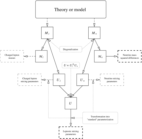
Figure 1: Flow-scheme for computing leptonic mixing parameters and lepton masses from any given charged lepton and neutrino mass matrices.

Note that our study assumes that there are three neutrino flavors, and therefore, three neutrino flavor states $\nu_{\alpha}$ ($\alpha=e,\mu,\tau$) and also three neutrino mass eigenstates $\nu_{a}$ ($a=1,2,3$). Furthermore, it assumes that all $\mathcal{CP}$ violation phases are equal to zero.

The paper is organized as follows: In Sec. 2, we introduce the representation content of our model including U(1) charges and discrete symmetries. The multi-scalar potential of the model is then analyzed in Sec. 3, where we explicitly demonstrate the vacuum alignment mechanism. Next, in Secs. 4 and 5, the Yukawa interactions of the charged leptons and neutrinos, respectively, are investigated and discussed, which lead to the mass matrices of the corresponding particles. In Sec. 6, the lepton mass matrices are diagonalized yielding the charged lepton masses and the neutrino mass squared differences as well as the charged lepton and neutrino mixing angles (see again Fig. 1). In Sec. 7, the total leptonic mixing angles are derived and calculated. Implications for neutrinoless double $\beta$-decay, astrophysics, and cosmology are briefly studied in Sec. 8. Finally, in Sec. 9, we present a summary as well as our conclusions. In addition, we present in the Appendix a scheme for how to transform any given $3\times 3$ unitary matrix to the “standard” parameterization form of the Particle Data Group [28].

2 The representation content

Let us consider an extension of the SM in which the lepton masses are generated by higher-dimensional operators [51, 52] via the Froggatt–Nielsen mechanism [53]. (A classification of effective neutrino mass operators has been given in Ref.[54].) Since we are mainly concerned with the question of whether there is a possible naturally maximal $\nu_{\mu}$-$\nu_{\tau}$-mixing in the MSW LMA solution or not, for which the properties of the quarks are seemingly irrelevant, we will, for simplicity and without loss of generality, omit the quark sector in our further discussion. For a recent related study including also the quark sector, see, e.g., Refs.[55, 56]. In a self-explanatory notation, we will denote the lepton doublets as $L_{\alpha}=(\begin{matrix}\nu_{\alpha L}&e_{\alpha L}\end{matrix})$, where $\alpha=e,\mu,\tau$, and the right-handed charged leptons as $E_{\alpha}=e_{\alpha R}$, where $\alpha=e,\mu,\tau$. The part of the scalar sector, which carries non-zero SM quantum numbers, consists of two Higgs doublets $H_{1}$ and $H_{2}$, where $H_{1}$ couples to the neutrinos and $H_{2}$ to the charged leptons. This can be achieved by assuming, e.g., a discrete ${\mathbb{Z}}_{2}$ symmetry under which $H_{2}$ and $E_{\alpha}$ ($\alpha=e,\mu,\tau$) are odd and $H_{1}$ and the rest of the SM fields are even. The masses of the charged leptons arise through the mixing with additional heavy right-handed charged fermions, which all have masses of the order of magnitude of some characteristic mass scale $M_{1}$. Apart from some general prescriptions of their transformations under the flavor symmetries, which will be introduced below, it is not necessary to explicitly present the fundamental theory of these additional (or extra) charged fermions. This is in contrast to the neutrino sector, which we will extend by five additional heavy SM singlet Dirac neutrinos $N_{e}$, $N_{\mu}$, $N_{\tau}$, $F_{1}$, and $F_{2}$. The neutrinos $F_{1}$ and $F_{2}$ are supposed to have masses of the same order $M_{1}$ as the charged intermediate Froggatt–Nielsen states, whereas $N_{e}$, $N_{\mu}$, and $N_{\tau}$ all have masses of the order of magnitude of some relevant high (unification) mass scale $M_{2}$. While $M_{2}$ takes the role of some seesaw scale [57, 58, 59] (and it is therefore responsible for the smallness of the neutrino masses), $M_{1}$ can be as low as several TeV [60, 61]. In order to obtain the structures of the lepton mass matrices from an underlying symmetry principle in the context of a renormalizable field theory, we will furthermore extend the scalar sector by additional SM singlet scalar fields $\phi_{1},\phi_{2},\ldots,\phi_{10}$, $\phi^{\prime}_{1},\phi^{\prime}_{2},\ldots,\phi^{\prime}_{6}$, and $\theta$ and we will assign these fields gauged horizontal U(1) charges $Q_{1}$, $Q_{2}$, and $Q_{3}$ as follows:

$$(Q_{1},Q_{2},Q_{3})$$

,

,,,

In the rest of the paper, it will always be understood that the Higgs doublets $H_{1}$ and $H_{2}$ are total singlet under transformations of other additional symmetries. Note that the charges $Q_{1}$ and $Q_{2}$ are anomalous. However, it is known that anomalous U(1) charges may arise in effective field theories from strings. Then, the cancellation of the anomalies must be accomplished by the Green–Schwarz mechanism [62].

The first generation of the charged leptons is distinguished from the second and third generations if we require for $P\equiv{\rm e}^{2\pi{\rm i}/n}$, where the integer $n$ obeys $n\geq 5$, invariance of the Lagrangian under transformation of the following ${\mathbb{Z}}_{n}$ symmetry:

$${\mathcal{D}}_{1} : \left\{\begin{matrix}E_{e}\rightarrow P^{-4}E_{e},&E_{\mu}\rightarrow P^{-1}E_{\mu},&E_{\tau}\rightarrow P^{-1}E_{\tau},\\ \phi_{1}\rightarrow P\phi_{1},&\phi_{2}\rightarrow P\phi_{2},\\ \phi_{3}\rightarrow P\phi_{3},&\phi_{4}\rightarrow P\phi_{4},\\ \phi_{5}\rightarrow P\phi_{5},&\phi_{6}\rightarrow P\phi_{6},\end{matrix}\right.$$ (1)

where we assume that the fields $N_{e}$, $N_{\mu}$, $N_{\tau}$, $F_{1}$, and $F_{2}$ are singlets under transformation of the symmetry ${\mathcal{D}}_{1}$. In addition, the symmetry ${\mathcal{D}}_{1}$ forbids the fields $\phi_{1},\phi_{2},\ldots,\phi_{6}$ to participate in the leading order mass terms for the neutrinos. Furthermore, the permutation symmetries

$${\mathcal{D}}_{2} : \left\{\begin{matrix}L_{\mu}\rightarrow-L_{\mu},&E_{\mu}\rightarrow-E_{\mu},\\ N_{\mu}\rightarrow-N_{\mu},&\\ \phi_{1}^{\prime}\leftrightarrow\phi_{2}^{\prime},&\phi_{1}\leftrightarrow\phi_{2},\\ \phi_{7}\rightarrow-\phi_{7},&\end{matrix}\right.$$ (2)

$${\mathcal{D}}_{3} : \left\{\begin{matrix}L_{\mu}\rightarrow-L_{\mu},&N_{\mu}\rightarrow-N_{\mu},\\ \phi_{3}^{\prime}\leftrightarrow\phi_{4}^{\prime},&\phi_{3}\leftrightarrow\phi_{4},\\ \phi_{5}^{\prime}\leftrightarrow\phi_{6}^{\prime},&\phi_{5}\leftrightarrow\phi_{6},\\ \phi_{7}\rightarrow-\phi_{7},\end{matrix}\right.$$ (3)

$${\mathcal{D}}_{4} : \left\{\begin{matrix}L_{\mu}\leftrightarrow L_{\tau},&E_{\mu}\leftrightarrow E_{\tau},\\ N_{\mu}\leftrightarrow N_{\tau},&\\ \phi_{2}\rightarrow-\phi_{2},&\phi_{4}\rightarrow-\phi_{4},&\phi_{6}\rightarrow-\phi_{6},\\ \phi_{7}\leftrightarrow\phi_{8}\end{matrix}\right.$$ (4)

are responsible for generating a naturally maximal atmospheric mixing angle, since they establish exact degeneracies of the Yukawa couplings in the leptonic 2-3-subsector. These permutation symmetries also play a crucial role in the scalar sector in which they restrict some of the couplings in the multi-scalar potential to be exactly degenerate (at tree level), which means that degenerate vacuum expectation values (VEVs) can emerge after spontaneous symmetry breaking (SSB). This so-called vacuum alignment mechanism can work if we assume the discrete symmetries

$${\mathcal{D}}_{5} : \left\{\begin{matrix}\phi_{1}^{\prime}\rightarrow-\phi_{1}^{\prime},&\phi_{1}\rightarrow-\phi_{1},\\ \phi_{3}^{\prime}\rightarrow-\phi_{3}^{\prime},&\phi_{3}\rightarrow-\phi_{3},\\ \phi_{5}^{\prime}\rightarrow-\phi_{5}^{\prime},&\phi_{5}\rightarrow-\phi_{5},\end{matrix}\right.$$ (5)

$${\mathcal{D}}_{6} : \left\{\begin{matrix}E_{e}\rightarrow P^{-(4l+1)}E_{e},&N_{e}\rightarrow PN_{e},\\ \phi_{1}^{\prime}\rightarrow P^{-k}\phi_{1}^{\prime},&\phi_{2}^{\prime}\rightarrow P^{-k}\phi_{2}^{\prime},\\ \phi_{3}^{\prime}\rightarrow P^{-l}\phi_{3}^{\prime},&\phi_{4}^{\prime}\rightarrow P^{-l}\phi_{4}^{\prime},\\ \phi_{5}^{\prime}\rightarrow P^{-m}\phi_{5}^{\prime},&\phi_{6}^{\prime}\rightarrow P^{-m}\phi_{6}^{\prime},\\ \phi_{1}\rightarrow P^{k}\phi_{1},&\phi_{2}\rightarrow P^{k}\phi_{2},\\ \phi_{3}\rightarrow P^{l}\phi_{3},&\phi_{4}\rightarrow P^{l}\phi_{4},\\ \phi_{5}\rightarrow P^{m}\phi_{5},&\phi_{6}\rightarrow P^{m}\phi_{6},\\ \phi_{9}\rightarrow P^{-1}\phi_{9},&\phi_{10}\rightarrow P\phi_{10},\end{matrix}\right.$$ (6)

where $k$, $l$, and $m$ are some integers. For the symmetry ${\mathcal{D}}_{6}$ we additionally require that the Froggatt–Nielsen states with non-zero hypercharge can only be multiplied by factors $P^{n}$, where $n$ is an integer multiple of $k$, $l$, or $m$, and that the differences $|k-l|$, $|k-m|$, and $|l-m|$ are sufficiently large. The only fermion with non-vanishing hypercharge that transforms differently is the right-handed electron $E_{e}$. These symmetries restrict the allowed combinations of the scalar fields in the higher-dimensional lepton mass operators as well as in the renormalizable terms of the multi-scalar potential. Thus, possibly dangerous terms in the multi-scalar potential can be forbidden, which could otherwise spoil the vacuum alignment mechanism.

At this stage, it is appropriate to point out some implications concerning the nature of the discrete symmetries. It has been found that relations between Yukawa couplings established by standard discrete symmetries can only remain unbroken by quantum gravity corrections if the discrete symmetries are gauged [63]. These “discrete gauge symmetries” appear in continuum theories when a gauge symmetry group $G$ is broken to a discrete symmetry subgroup $H$. Since acceptable continuous gauge theories have to be free from chiral anomalies, one obtains discrete anomaly cancellation conditions, which strongly constrain the massless fermion content of the theory [64]. At a more fundamental level, this implies for our model that the permutation symmetries must actually be gauged, since the relations, which are based on them, will prove to be crucial for obtaining essentially strict maximal atmospheric mixing. However, it is interesting to note that in $M$-theory, one expects the discrete symmetries to be always anomaly-free [65].

3 The multi-scalar potential

3.1 The two-Higgs doublet potential

From the most general two-Higgs doublet potential of the fields $H_{1}$ and $H_{2}$ (for an extensive review on electroweak Higgs potentials, see, e.g., Ref.[66]) we conclude that, in presence of the ${\mathbb{Z}}_{2}$ symmetry, which distinguishes between $H_{1}$ and $H_{2}$ (see Sec. 2), each of these fields appears only to the second or fourth power in the multi-scalar potential. Hence, in any renormalizable terms of the multi-scalar potential, which mix $H_{1}$ or $H_{2}$ with the SM singlet scalar fields, the Higgs doublets are only allowed to appear in terms of their absolute squares $|H_{1}|^{2}$ and $|H_{2}|^{2}$. Next, since the Higgs doublets carry zero $Q_{1},Q_{2},$ and $Q_{3}$ charges and are ${\mathcal{D}}_{i}$-singlets, where $i=1,2,\ldots,6$, there exists a range of parameters in the multi-scalar potential for which the standard two-Higgs electroweak symmetry breaking is possible. Furthermore, this implies that we can, without loss of generality, separate the SM singlet scalar part from the Higgs-doublet part in the multi-scalar potential by formally absorbing the absolute squares of the VEVs $|\langle H_{1}\rangle|^{2}$ and $|\langle H_{2}\rangle|^{2}$ into the coupling constants of the mixed terms. Then, since the vacuum alignment mechanism of the SM singlet fields is independent from the details of the Higgs doublet physics, we can in what follows discard the effects of the Higgs doublets and fully concentrate on the properties of the SM singlet scalar fields.

3.2 Interactions of the fields $\phi_{9}$ and $\phi_{10}$

The symmetry ${\mathcal{D}}_{6}$ requires that the fields $\phi_{9}$ and $\phi_{10}$ enter the renormalizable interactions of the scalar fields only in terms of the operators $\phi_{9}\phi_{10},\phi_{9}^{\dagger}\phi_{10}^{\dagger},|\phi_{9}|^{2}$, and $|\phi_{10}|^{2}$. The product $\phi_{9}\phi_{10}$ has the U(1) charge structure $(-2,0,1)$, implying that the only renormalizable interaction in the scalar potential, which involves this product, is actually $\sim|\phi_{9}|^{2}|\phi_{10}|^{2}$. We can assume that both of the fields $\phi_{9}$ and $\phi_{10}$ finally develop non-vanishing VEVs with magnitudes $|\langle\phi_{9}\rangle|$ and $|\langle\phi_{10}\rangle|$ that are not too large. Since the fields $\phi_{9}$ and $\phi_{10}$ are singlets under transformations of all the permutation symmetries ${\mathcal{D}}_{2},{\mathcal{D}}_{3}$, and ${\mathcal{D}}_{4}$, they will have no effect on the relative alignment of the rest of the scalar fields, because they enter the corresponding interactions only in terms of the absolute squares $|\langle\phi_{9}\rangle|^{2}$ and $|\langle\phi_{10}\rangle|^{2}$. For this reason we will, without loss of generality, discard the terms in the scalar potential which involve the fields $\phi_{9}$ and $\phi_{10}$ in our considerations.

From the assignment of the U(1) charges $Q_{1},Q_{2}$, and $Q_{3}$ and the symmetry ${\mathcal{D}}_{6}$ (which does not permute any of the fields) it follows that any renormalizable term in the scalar potential which involves the SM singlet fields $\phi_{1},\phi_{2},\phi_{5},\phi_{6},\phi_{7},\phi_{8}$, or $\theta$ can only be allowed if these fields appear in one of the following combinations:

$$\phi_{1,2}\phi_{1,2}^{\dagger}\>,\quad\phi_{5,6}\phi_{5,6}^{\dagger}\>,\quad\phi_{5,6}\theta\>,\quad\phi_{7,8}\phi_{7,8}^{\dagger}\>,\quad|\theta|^{2}\>,$$ (7)

where “$\phi_{i,j}$” ($i,j=1,2,\dots,8$) denotes some linear combination of the fields $\phi_{i}$ and $\phi_{j}$. Among the products in Eq. (7) only the product $\phi_{5,6}\theta$ transforms non-trivially under the symmetry ${\mathcal{D}}_{1}$. In addition, since the fields $\phi_{1}^{\prime},\phi_{2}^{\prime},\ldots,\phi_{6}^{\prime}$ are ${\mathcal{D}}_{1}$-singlets, we observe that the fields $\phi_{3}$ and $\phi_{4}$, which carry a non-zero ${\mathcal{D}}_{1}$-charge, can only appear either in the combination $\phi_{3,4}\phi_{3,4}^{\dagger}$ or in the combination $\phi_{3,4}^{\dagger}\phi_{5,6}\theta$. However, the latter combination is forbidden by $\mathcal{D}_{6}$-invariance.

3.3 Interactions of the field $\theta$

As in Sec. 3.2, we can assume that the field $\theta$ finally develops a non-vanishing VEV with a magnitude $|\langle\theta\rangle|$ that is not too large. Except for the combination $\phi_{5,6}\theta$ in Eq. (7) all scalar interactions involve an equal number (0, 1, or 2) of the fields $\theta$ and its adjoint $\theta^{\dagger}$, which can then be paired to the absolute square $|\theta|^{2}$. Since the interaction $\phi_{5,6}\theta|\theta|^{2}$ is forbidden by the symmetries ${\mathcal{D}}_{1}$ and ${\mathcal{D}}_{6}$ and $\theta$ is a total singlet under transformations of the discrete symmetries ${\mathcal{D}}_{1},{\mathcal{D}}_{2},\ldots,{\mathcal{D}}_{6}$, all terms which involve the absolute square $|\theta|^{2}$ will have no influence on the relative alignment of the rest of the scalar fields. For this reason we can, without loss of generality, omit the terms in the scalar potential which involve $|\theta|^{2}$ in our considerations.

3.4 Interactions of the fields $\phi_{7}$ and $\phi_{8}$

From the U(1) charge assignment we conclude that only an even number of the fields $\phi_{7}$ and $\phi_{8}$ (or their complex conjugates) can participate in the scalar interactions. Let us now especially consider the operator $\phi_{7}^{\dagger}\phi_{8}$ (or equivalently its complex conjugate). Under application of each of the symmetries ${\mathcal{D}}_{2}$ and ${\mathcal{D}}_{3}$ the operator $\phi_{7}^{\dagger}\phi_{8}$ changes sign. Therefore, the symmetry ${\mathcal{D}}_{2}$ requires this operator to couple to one of the fields taken from the set $\{\phi_{1}^{\prime},\phi_{2}^{\prime},\phi_{1},\phi_{2},\phi_{7}\}$. Simultaneously, the symmetry ${\mathcal{D}}_{3}$ requires this operator to couple only to fields taken from the extended set $\{\phi_{3}^{\prime},\phi_{4}^{\prime},\phi_{5}^{\prime},\phi_{6}^{\prime},\phi_{3},\phi_{4},\phi_{5},\phi_{6},\phi_{7}\}$. Both conditions can only be fulfilled if the operator $\phi_{7}^{\dagger}\phi_{8}$ couples to the field $\phi_{7}$ or its complex conjugate, but not to the operator products $(\phi_{7})^{2},(\phi_{7}^{\dagger})^{2}$, or $|\phi_{7}|^{2}$. Since the product $\phi_{7}^{\dagger}\phi_{8}$ carries the U(1) charges $(0,0,0)$, the operator $\phi_{7}^{\dagger}\phi_{8}$ can only couple to some linear combination of the operators $\phi_{7}\phi_{8}^{\dagger}$ and $\phi_{8}\phi_{7}^{\dagger}$. As a consequence, if a general operator $\phi_{7,8}\phi_{7,8}^{\dagger}$ enters an interaction with scalars, which are different from the fields $\phi_{7}$ and $\phi_{8}$, then this operator $\phi_{7,8}\phi_{7,8}^{\dagger}$ is a linear combination of the absolute squares $|\phi_{7}|^{2}$ and $|\phi_{8}|^{2}$.

Let us denote by $\phi_{i}$ and $\phi_{j}$ two scalar fields, which are different from the fields $\phi_{7}$ and $\phi_{8}$. Taking Eq. (7) and the operator $\phi_{3,4}\phi_{3,4}^{\dagger}$ into account, the operator product $\phi_{i}\phi_{j}$ must be of one of the following types:

$$\phi_{1,2}\phi_{1,2}^{\dagger}\>,\quad\phi_{3,4}\phi_{3,4}^{\dagger}\>,\quad\phi_{5,6}\phi_{5,6}^{\dagger}\>,\quad\phi_{1,2}^{\prime}{\phi^{\prime}}^{\dagger}_{1,2}\>,\quad\phi_{3,4}^{\prime}{\phi^{\prime}}_{3,4}^{\dagger}\>,\quad\phi_{5,6}^{\prime}{\phi^{\prime}}_{5,6}^{\dagger}\>,$$ (8)

where the last three combinations follow from the ${\mathcal{D}}_{6}$-invariance. Next, the symmetry ${\mathcal{D}}_{5}$ implies that $\phi_{j}=\phi_{i}^{\dagger}$ for the combinations in Eq. (8), i.e., the product is the absolute square $\phi_{i}\phi_{j}=|\phi_{i}|^{2}$. Using the result of the previous paragraph, invariance under transformation of the symmetry ${\mathcal{D}}_{4}$ gives for the most general interactions of the fields $\phi_{7}$ and $\phi_{8}$ with the other scalar fields the terms

$$(|\phi_{7}|^{2}+|\phi_{8}|^{2})\sum_{\varphi_{i}\neq\phi_{7},\phi_{8}}c_{i}|\varphi_{i}|^{2},$$ (9)

where $\varphi_{i}$ can be any of the scalar fields, which are not identical with the fields $\phi_{7}$ or $\phi_{8}$ and $c_{i}$ are some real-valued coupling constants. (Dimension-three terms of the types $|\phi_{7}|^{2}\varphi_{i}$ or $|\phi_{8}|^{2}\varphi_{i}$, where $\varphi_{i}\neq\phi_{7},\phi_{8}$, are forbidden by the U(1) charge assignment and the symmetry ${\mathcal{D}}_{6}$, which does not permute any fields.) Taking everything into account, the U(1) charge assignment and the symmetry ${\mathcal{D}}_{4}$ restrict the most general terms in the scalar potential, involving the fields $\phi_{7}$ and $\phi_{8}$, to be

$$V_{7,8} = \mu^{2}(|\phi_{7}|^{2}+|\phi_{8}|^{2})+\kappa(|\phi_{7}|^{2}+|\phi_{8}|^{2})^{2}+(|\phi_{7}|^{2}+|\phi_{8}|^{2})\sum_{\varphi_{i}\neq\phi_{7},\phi_{8}}c_{i}|\varphi_{i}|^{2}$$ (10)

$$+ a\left[(\phi_{7}^{\dagger}\phi_{8})^{2}+(\phi_{8}^{\dagger}\phi_{7})^{2}\right]+b|\phi_{7}|^{2}|\phi_{8}|^{2},$$

where $\mu^{2}$, $\kappa$, $a$, and $b$ are real-valued constants. Parameterizing the VEVs of $\phi_{7}$ and $\phi_{8}$ as

$$\left(\begin{array}[]{c}\langle\phi_{7}\rangle\\ \langle\phi_{8}\rangle\end{array}\right)=v\left(\begin{array}[]{c}{\rm e}^{{\rm i}\beta_{1}}\cos\alpha\\ {\rm e}^{{\rm i}\beta_{2}}\sin\alpha\end{array}\right),$$ (11)

where $v$ is some real-valued number, $\alpha$ is the angle which rotates $\langle\phi_{7}\rangle$ and $\langle\phi_{8}\rangle$, and $\beta_{1}$ and $\beta_{2}$ denote the phases of the VEVs, we observe in Eq. (10) that the first three terms exhibit an accidental ${\rm U(1)}_{\alpha}$ symmetry. This symmetry is broken by the last two terms, which are therefore responsible for the alignment of the VEVs. Note that the scalar potential is symmetric under the exchange $\phi_{7}\leftrightarrow\phi_{8}$ and that the term with coefficient $a$ is $\sim\Re\left[(\phi_{7}^{\dagger}\phi_{8})^{2}\right]$. In Eq. (10), we will choose $\kappa>0$ and assume the rest of the coupling constants to be negative. Then, the lowest energy state is characterized by $\alpha=\tfrac{\pi}{4}$ and $\beta_{1}-\beta_{2}\in\{0,\pi\}$ or equivalently

$$\langle\phi_{7}\rangle=\pm\langle\phi_{8}\rangle,$$ (12)

i.e., the VEVs are degenerate up to a sign. When considering the Yukawa interactions of the neutrinos, it will turn out that the degeneracy of the VEVs is responsible for a nearly maximal atmospheric mixing angle. Thus, we can from now on restrict our discussion of the scalar potential to the fields $\phi_{1},\phi_{2},\ldots,\phi_{6}$, and $\phi_{1}^{\prime},\phi_{2}^{\prime},\ldots,\phi_{6}^{\prime}$. This discussion will follow in the three coming subsections.

3.5 The potential of the fields $\phi_{1},\phi_{2},\ldots,\phi_{6}$

In all two-fold and four-fold products involving only the fields $\phi_{i}$ ($i=1,2,\ldots,6$), the discrete symmetry $\mathcal{D}_{5}$ requires the number of these fields, which are denoted by even (or odd) indices, to be even. In the scalar potential, linear and tri-linear terms of the fields $\phi_{1},\phi_{2},\ldots,\phi_{6}$ are forbidden by the symmetry ${\mathcal{D}}_{6}$. Taking the combinations in Eq. (7) and $\phi_{3,4}\phi_{3,4}^{\dagger}$ into account, the allowed two-fold products of the fields $\phi_{1},\phi_{2},\ldots,\phi_{6}$ can only be of the type $|\phi_{i}|^{2}$, i.e., they must be absolute squares of the fields. Similarly, we obtain that all four-fold products of the fields $\phi_{1},\phi_{2},\ldots,\phi_{6}$ must be of the types

$$(\phi_{1}\phi_{2}^{\dagger})^{2}\>,\quad\phi_{1}\phi_{2}^{\dagger}\phi_{3}\phi_{4}^{\dagger}\>,\quad\phi_{1}\phi_{2}^{\dagger}\phi_{4}\phi_{3}^{\dagger}\>,\quad\phi_{1}\phi_{2}^{\dagger}\phi_{5}\phi_{6}^{\dagger}\>,\quad\phi_{1}\phi_{2}^{\dagger}\phi_{6}\phi_{5}^{\dagger}\>,$$ (13)

$$(\phi_{3}\phi_{4}^{\dagger})^{2}\>,\quad\phi_{3}\phi_{4}^{\dagger}\phi_{5}\phi_{6}^{\dagger}\>,\quad\phi_{3}\phi_{4}^{\dagger}\phi_{6}\phi_{5}^{\dagger}\>,\quad(\phi_{5}\phi_{6}^{\dagger})^{2}\>,\quad|\phi_{i}|^{2}|\phi_{j}|^{2}\>,\quad|\phi_{i}|^{4}\>,$$

and their complex conjugates, where $i,j=1,2,\ldots,6$. A general four-fold product of the types in Eq. (13) can be written as

$$(a\phi_{i}^{\dagger}\phi_{j}+b\phi_{j}^{\dagger}\phi_{i})\phi_{k}^{\dagger}\phi_{l}+(c\phi_{i}^{\dagger}\phi_{j}+d\phi_{j}^{\dagger}\phi_{i})\phi_{l}^{\dagger}\phi_{k}+{\rm h.c.}$$

$$= \left[(a+d^{\ast})\phi_{i}^{\dagger}\phi_{j}+(b+c^{\ast})\phi_{j}^{\dagger}\phi_{i}\right]\phi_{k}^{\dagger}\phi_{l}+\left[(c+b^{\ast})\phi_{i}^{\dagger}\phi_{j}+(d+a^{\ast})\phi_{j}^{\dagger}\phi_{i}\right]\phi_{l}^{\dagger}\phi_{k},$$

where $a,b,c$, and $d$ are complex-valued constants. Assume that $i\neq j$. Then, from Eq. (13) we observe that $k\neq l$ and we can, without loss of generality, assume that the index-pairs $(i,j)$ and $(k,l)$, respectively, combine the fields which are interchanged by the discrete symmetry ${\mathcal{D}}_{2}$ or ${\mathcal{D}}_{3}$. (If $i=j$, then it follows from Eq. (13) that $k=l$, which will be discussed below.) Let, in addition, $\{i,j\}\neq\{k,l\}$. Then, application of the symmetries ${\mathcal{D}}_{2}$ and ${\mathcal{D}}_{3}$ yields $a+d^{\ast}=d+a^{\ast}$ and $b+c^{\ast}=c+b^{\ast}$. We can therefore rename the constants as $a+d^{\ast}\rightarrow a$ and $b+c^{\ast}\rightarrow b$, where now $a$ and $b$ are real constants, and write the term in Eq. (3.5) as

$$(a\phi_{i}^{\dagger}\phi_{j}+b\phi_{j}^{\dagger}\phi_{i})\phi_{k}^{\dagger}\phi_{l}+(b\phi_{i}^{\dagger}\phi_{j}+a\phi_{j}^{\dagger}\phi_{i})\phi_{l}^{\dagger}\phi_{k}$$ (15)

$$= \frac{a+b}{2}(\phi_{i}^{\dagger}\phi_{j}+\phi_{j}^{\dagger}\phi_{i})(\phi_{k}^{\dagger}\phi_{l}+\phi_{l}^{\dagger}\phi_{k})+\frac{a-b}{2}(\phi_{i}^{\dagger}\phi_{j}-\phi_{j}^{\dagger}\phi_{i})(\phi_{k}^{\dagger}\phi_{l}-\phi_{l}^{\dagger}\phi_{k})$$

$$= \frac{a+b}{2}\>\Re(\phi_{i}^{\dagger}\phi_{j})\>\Re(\phi_{k}^{\dagger}\phi_{l})-\frac{a-b}{2}\>\Im(\phi_{i}^{\dagger}\phi_{j})\>\Im(\phi_{k}^{\dagger}\phi_{l}).$$

Since the fields $\phi_{3},\phi_{4},\phi_{5}$, and $\phi_{6}$ are singlets under transformation of the discrete symmetry ${\mathcal{D}}_{2}$, we can have $a\neq b$ in the case that $(\phi_{i},\phi_{j})=(\phi_{3},\phi_{4})$ and $(\phi_{k},\phi_{l})=(\phi_{5},\phi_{6})$. However, if $(i,j)=(1,2)$, then application of the discrete symmetry ${\mathcal{D}}_{2}$ further constrains the constants in the above general form to fulfill $a=b$, and therefore, the last term in Eq. (15) vanishes.

As a cause of the symmetries ${\mathcal{D}}_{2}$ and ${\mathcal{D}}_{3}$, the products $(\phi_{i}\phi_{j}^{\dagger})^{2}$ in Eq. (13), where $(i,j)=(1,2),(3,4),(5,6)$, appear in the potential always as

$$a\left[(\phi_{i}\phi_{j}^{\dagger})^{2}+(\phi_{j}^{\dagger}\phi_{i})^{2}\right]=2a\Re\left[(\phi_{i}\phi_{j}^{\dagger})^{2}\right],$$ (16)

where $a$ is some real-valued constant.

Let us now turn the discussion to the terms $|\phi_{i}|^{2}|\phi_{k}|^{2}$ in Eq. (13), where $i\neq k$. Assume that the fields $\phi_{i}$ and $\phi_{k}$ cannot be combined into one of the pairs $(\phi_{1},\phi_{2}),(\phi_{3},\phi_{4})$, or $(\phi_{5},\phi_{6})$. Then, a general term of this type is on the form

$$(a|\phi_{i}|^{2}+b|\phi_{j}|^{2})|\phi_{k}|^{2}+(c|\phi_{i}|^{2}+d|\phi_{j}|^{2})|\phi_{l}|^{2},$$ (17)

where $a,b,c$, and $d$ are real-valued constants and
$(\phi_{i},\phi_{j}),(\phi_{k},\phi_{l})\in\{(1,2),(3,4),(5,6)\}$. Application of the symmetries ${\mathcal{D}}_{2}$ and ${\mathcal{D}}_{3}$ yields the conditions $a=d$ and $b=c$, and thus, we can rewrite the above part of the potential as

$$\frac{a+b}{2}(|\phi_{i}|^{2}+|\phi_{j}|^{2})(|\phi_{k}|^{2}+|\phi_{l}|^{2})+\frac{a-b}{2}(|\phi_{i}|^{2}-|\phi_{j}|^{2})(|\phi_{k}|^{2}-|\phi_{l}|^{2}).$$ (18)

If $(i,j)=(3,4)$ and $(k,l)=(5,6)$, then in general $a\neq b$, since the fields $\phi_{3},\phi_{4},\phi_{5}$, and $\phi_{6}$ are ${\mathcal{D}}_{2}$-singlets. However, if $(i,j)=(1,2)$, then $a=b$ and the part in Eq. (18) which is proportional to $(a-b)/2$ vanishes.

If in the combination $|\phi_{i}|^{2}|\phi_{j}|^{2}$ in Eq. (13) the fields $(\phi_{i},\phi_{j})$ form one of the pairs $(\phi_{1},\phi_{2}),(\phi_{3},\phi_{4})$, or $(\phi_{5},\phi_{6})$, then the combination $|\phi_{i}|^{2}|\phi_{j}|^{2}$ is a total singlet (on its own) and it can be written directly into the scalar potential as $a|\phi_{i}|^{2}|\phi_{j}|^{2}$, where $a$ is some real-valued constant.

Moreover, the symmetries ${\mathcal{D}}_{2}$ and ${\mathcal{D}}_{3}$ enforce the products $|\phi_{i}|^{2}$ and $|\phi_{i}|^{4}$ [in Eq. (13)] to appear in the scalar potential only as

$$\mu_{1}^{2}\left(|\phi_{1}|^{2}+|\phi_{2}|^{2}\right)+\mu_{2}^{2}\left(|\phi_{3}|^{2}+|\phi_{4}|^{2}\right)+\mu_{3}^{2}\left(|\phi_{5}|^{2}+|\phi_{6}|^{2}\right)$$ (19)

$$+ \kappa_{1}\left(|\phi_{1}|^{4}+|\phi_{2}|^{4}\right)+\kappa_{2}\left(|\phi_{3}|^{4}+|\phi_{4}|^{4}\right)+\kappa_{3}\left(|\phi_{5}|^{4}+|\phi_{6}|^{4}\right),$$

where $\mu_{1}^{2}$, $\mu_{2}^{2}$, $\mu_{3}^{2}$, $\kappa_{1}$, $\kappa_{2}$, and $\kappa_{3}$ are real-valued constants. In total, the most general scalar potential involving only the unprimed fields, but neither the fields $\phi_{7}$, $\phi_{8}$, $\phi_{9}$, and $\phi_{10}$ nor the product $|\theta|^{2}$, reads

$$V_{1} = \mu_{1}^{2}\left(|\phi_{1}|^{2}+|\phi_{2}|^{2}\right)+\mu_{2}^{2}\left(|\phi_{3}|^{2}+|\phi_{4}|^{2}\right)+\mu_{3}^{2}\left(|\phi_{5}|^{2}+|\phi_{6}|^{2}\right)$$

$$+ \kappa_{1}\left(|\phi_{1}|^{2}+|\phi_{2}|^{2}\right)^{2}+\kappa_{2}\left(|\phi_{3}|^{2}+|\phi_{4}|^{2}\right)^{2}+\kappa_{3}\left(|\phi_{5}|^{2}+|\phi_{6}|^{2}\right)^{2}$$

$$+ d_{1}\left(|\phi_{1}|^{2}+|\phi_{2}|^{2}\right)\left(|\phi_{3}|^{2}+|\phi_{4}|^{2}\right)+d_{2}\left(|\phi_{1}|^{2}+|\phi_{2}|^{2}\right)\left(|\phi_{5}|^{2}+|\phi_{6}|^{2}\right)$$

$$+ d_{3}\left(|\phi_{3}|^{2}+|\phi_{4}|^{2}\right)\left(|\phi_{5}|^{2}+|\phi_{6}|^{2}\right)+d_{4}\left(|\phi_{3}|^{2}-|\phi_{4}|^{2}\right)\left(|\phi_{5}|^{2}-|\phi_{6}|^{2}\right)$$

$$+ d_{5}|\phi_{1}^{\dagger}\phi_{2}|^{2}+d_{6}|\phi_{3}^{\dagger}\phi_{4}|^{2}+d_{7}|\phi_{5}^{\dagger}\phi_{6}|^{2}+d_{8}\left[(\phi_{1}^{\dagger}\phi_{2})^{2}+(\phi_{2}^{\dagger}\phi_{1})^{2}\right]$$

$$+ d_{9}\left[(\phi_{3}^{\dagger}\phi_{4})^{2}+(\phi_{4}^{\dagger}\phi_{3})^{2}\right]+d_{10}\left[(\phi_{5}^{\dagger}\phi_{6})^{2}+(\phi_{6}^{\dagger}\phi_{5})^{2}\right]$$

$$+ d_{11}\left(\phi_{1}^{\dagger}\phi_{2}+\phi_{2}^{\dagger}\phi_{1}\right)\left(\phi_{3}^{\dagger}\phi_{4}+\phi_{4}^{\dagger}\phi_{3}\right)$$

$$+ d_{12}\left(\phi_{1}^{\dagger}\phi_{2}+\phi_{2}^{\dagger}\phi_{1}\right)\left(\phi_{5}^{\dagger}\phi_{6}+\phi_{6}^{\dagger}\phi_{5}\right)$$

$$+ d_{13}\left(\phi_{3}^{\dagger}\phi_{4}+\phi_{4}^{\dagger}\phi_{3}\right)\left(\phi_{5}^{\dagger}\phi_{6}+\phi_{6}^{\dagger}\phi_{5}\right)$$

$$+ d_{14}\left(\phi_{3}^{\dagger}\phi_{4}-\phi_{4}^{\dagger}\phi_{3}\right)\left(\phi_{5}^{\dagger}\phi_{6}-\phi_{6}^{\dagger}\phi_{5}\right),$$

where $d_{1},d_{2},\ldots,d_{14}$ are real-valued constants. We will assume that $\kappa_{1},\kappa_{2},\kappa_{3}>0$ and $d_{11},d_{13}>0$ and we will choose all other coupling constants to be negative. Again, we observe that the first nine terms in Eq. (LABEL:eq:V1) exhibit three accidental U(1) symmetries, which act on the pairs of VEVs $(\langle\phi_{1}\rangle,\langle\phi_{2}\rangle)$, $(\langle\phi_{3}\rangle,\langle\phi_{4}\rangle)$, and $(\langle\phi_{5}\rangle,\langle\phi_{6}\rangle)$, respectively. The rest of the terms in the potential $V_{1}$ break these symmetries and will therefore determine the vacuum alignment mechanism of the fields. First, we note that the term with the coefficient $d_{4}$ tends (for large values of $|d_{4}|$) to induce a splitting between $|\langle\phi_{3}\rangle|$ and $|\langle\phi_{4}\rangle|$ as well as between $|\langle\phi_{5}\rangle|$ and $|\langle\phi_{6}\rangle|$. Second, we observe that the term with the coefficient $d_{14}$ has (for large values of $|d_{14}|$) the tendency to trigger relative phases (different from $0$ and $\pi$) between $\langle\phi_{3}\rangle$ and $\langle\phi_{4}\rangle$ as well as between $\langle\phi_{5}\rangle$ and $\langle\phi_{6}\rangle$. However, if we require that

$$d_{6}d_{7}>4d_{4}^{2}\quad\mbox{and}\quad d_{9}d_{10}>4d_{14}^{2},$$ (21)

then the potential $V_{1}$ is minimized by the VEVs of the unprimed fields, which are pairwise degenerate in their magnitudes, i.e., they satisfy

$$|\langle\phi_{1}\rangle|=|\langle\phi_{2}\rangle|,\quad|\langle\phi_{3}\rangle|=|\langle\phi_{4}\rangle|,\quad|\langle\phi_{5}\rangle|=|\langle\phi_{6}\rangle|$$ (22a)

and are also pairwise relatively real, i.e.,

$$\frac{\langle\phi_{1}\rangle}{\langle\phi_{2}\rangle},\frac{\langle\phi_{3}\rangle}{\langle\phi_{4}\rangle},\frac{\langle\phi_{5}\rangle}{\langle\phi_{6}\rangle}\in\{-1,1\},$$ (22b)

where, in addition, the choice $$d_{12}<0 d_{11},d_{13}>0$$ and implies a correlation between the different pairs of VEVs in terms of

$$\frac{\langle\phi_{1}\rangle}{\langle\phi_{2}\rangle}\frac{\langle\phi_{5}\rangle}{\langle\phi_{6}\rangle}=1\quad\mbox{and}\quad\frac{\langle\phi_{1}\rangle}{\langle\phi_{2}\rangle}\frac{\langle\phi_{3}\rangle}{\langle\phi_{4}\rangle}=-1,$$ (22c)

i.e., the relative sign between $\langle\phi_{1}\rangle$ and $\langle\phi_{2}\rangle$ is equal to the relative sign between $\langle\phi_{5}\rangle$ and $\langle\phi_{6}\rangle$ and opposite to the relative sign between $\langle\phi_{3}\rangle$ and $\langle\phi_{4}\rangle$.

3.6 The potential of the fields $\phi_{1}^{\prime},\phi_{2}^{\prime},\ldots,\phi_{6}^{\prime}$

The only two-fold products of the primed fields $\phi_{i}^{\prime}$ ($i=1,2,\ldots,6$) which are allowed by the discrete symmetries ${\mathcal{D}}_{1},{\mathcal{D}}_{5}$, and ${\mathcal{D}}_{6}$ are the absolute squares $|\phi_{i}^{\prime}|^{2}$. Furthermore, the permutation symmetries ${\mathcal{D}}_{2}$ and ${\mathcal{D}}_{3}$ yield for the most general dimension-two terms of the primed fields the expression

$$\mu_{4}^{2}(|\phi_{1}^{\prime}|^{2}+|\phi_{2}^{\prime}|^{2})+\mu_{5}^{2}(|\phi_{3}^{\prime}|^{2}+|\phi_{4}^{\prime}|^{2})+\mu_{6}^{2}(|\phi_{5}^{\prime}|^{2}+|\phi_{6}^{\prime}|^{2}),$$ (23)

where $\mu_{4}^{2}$, $\mu_{5}^{2}$, and $\mu_{6}^{2}$ are real-valued constants. The permutation symmetries ${\mathcal{D}}_{2}$ and ${\mathcal{D}}_{3}$ additionally require the most general products of the absolute squares $|\phi^{\prime}_{i}|^{2}$ to be

$$\kappa_{4}\left(|\phi_{1}^{\prime}|^{2}+|\phi_{2}^{\prime}|^{2}\right)^{2}+\kappa_{5}\left(|\phi_{3}^{\prime}|^{2}+|\phi_{4}^{\prime}|^{2}\right)^{2}+\kappa_{6}\left(|\phi_{5}^{\prime}|^{2}+|\phi_{6}^{\prime}|^{2}\right)^{2}$$ (24)

$$+ a_{1}\left(|\phi_{1}^{\prime}|^{2}+|\phi_{2}^{\prime}|^{2}\right)\left(|\phi_{3}^{\prime}|^{2}+|\phi_{4}^{\prime}|^{2}\right)+a_{2}\left(|\phi_{1}^{\prime}|^{2}+|\phi_{2}^{\prime}|^{2}\right)\left(|\phi_{5}^{\prime}|^{2}+|\phi_{6}^{\prime}|^{2}\right)$$

$$+ a_{3}\left(|\phi_{3}^{\prime}|^{2}+|\phi_{4}^{\prime}|^{2}\right)\left(|\phi_{5}^{\prime}|^{2}+|\phi_{6}^{\prime}|^{2}\right)+a_{4}\left(|\phi_{3}^{\prime}|^{2}-|\phi_{4}^{\prime}|^{2}\right)\left(|\phi_{5}^{\prime}|^{2}-|\phi_{6}^{\prime}|^{2}\right)$$

$$+ a_{5}|{\phi_{1}^{\prime}}^{\dagger}\phi_{2}^{\prime}|^{2}+a_{6}|{\phi_{3}^{\prime}}^{\dagger}\phi_{4}^{\prime}|^{2}+a_{7}|{\phi_{5}^{\prime}}^{\dagger}\phi_{6}^{\prime}|^{2},$$

where $\kappa_{4}$, $\kappa_{5}$, $\kappa_{6}$, and $a_{1},a_{2},\ldots,a_{7}$ are real-valued constants. Note that three-fold products of the primed fields are forbidden by the ${\mathcal{D}}_{6}$-charge assignment. The discrete symmetry ${\mathcal{D}}_{6}$ requires that the remaining interactions of the primed fields can be written as products of the operators ${\phi^{\prime}}_{1}^{\dagger}\phi^{\prime}_{2}$, ${\phi^{\prime}}_{3}^{\dagger}\phi^{\prime}_{4}$, and ${\phi^{\prime}}_{5}^{\dagger}\phi^{\prime}_{6}$ (and their complex conjugates). Hence, the operators which involve the fields of only one of the pairs $(\phi_{1}^{\prime},\phi_{2}^{\prime})$, $(\phi_{3}^{\prime},\phi_{4}^{\prime})$, or $(\phi_{5}^{\prime},\phi_{6}^{\prime})$ are restricted by the symmetries ${\mathcal{D}}_{3}$ and ${\mathcal{D}}_{4}$ to be on the form

$$a_{8}\left[({\phi_{1}^{\prime}}^{\dagger}\phi_{2}^{\prime})^{2}+({\phi_{2}^{\prime}}^{\dagger}{\phi_{1}^{\prime}})^{2}\right]+a_{9}\left[({\phi_{3}^{\prime}}^{\dagger}\phi_{4}^{\prime})^{2}+({\phi_{4}^{\prime}}^{\dagger}\phi_{3}^{\prime})^{2}\right]$$ (25)

$$+ a_{10}\left[({\phi_{5}^{\prime}}^{\dagger}\phi_{6}^{\prime})^{2}+({\phi_{6}^{\prime}}^{\dagger}\phi_{5}^{\prime})^{2}\right]$$

$$= 2a_{8}\Re\left[({\phi_{1}^{\prime}}^{\dagger}{\phi_{2}^{\prime}})^{2}\right]+2a_{9}\Re\left[({\phi_{3}^{\prime}}^{\dagger}\phi_{4}^{\prime})^{2}\right]+2a_{10}\Re\left[({\phi_{5}^{\prime}}^{\dagger}\phi_{6}^{\prime})^{2}\right],$$

where $a_{8}$, $a_{9}$, and $a_{10}$ are real-valued constants. Furthermore, the symmetries ${\mathcal{D}}_{2},{\mathcal{D}}_{3},{\mathcal{D}}_{5}$, and ${\mathcal{D}}_{6}$ restrict the only dimension-four terms involving at least three different primed fields (or their complex conjugates) to be

$$a_{11}\left({\phi_{1}^{\prime}}^{\dagger}\phi^{\prime}_{2}+{\phi_{2}^{\prime}}^{\dagger}\phi_{1}^{\prime}\right)\left({\phi_{3}^{\prime}}^{\dagger}\phi_{4}^{\prime}+{\phi_{4}^{\prime}}^{\dagger}\phi_{3}^{\prime}\right)$$ (26)

$$+ a_{12}\left({\phi_{1}^{\prime}}^{\dagger}\phi_{2}^{\prime}+{\phi_{2}^{\prime}}^{\dagger}{\phi_{1}^{\prime}}\right)\left({\phi_{5}^{\prime}}^{\dagger}{\phi_{6}^{\prime}}+{\phi_{6}^{\prime}}^{\dagger}{\phi_{5}^{\prime}}\right)$$

$$+ a_{13}\left({\phi_{3}^{\prime}}^{\dagger}{\phi_{4}^{\prime}}+{\phi_{4}^{\prime}}^{\dagger}{\phi_{3}^{\prime}}\right)\left({\phi_{5}^{\prime}}^{\dagger}{\phi_{6}^{\prime}}+{\phi_{6}^{\prime}}^{\dagger}{\phi_{5}^{\prime}}\right)$$

$$+ a_{14}\left({\phi_{3}^{\prime}}^{\dagger}{\phi_{4}^{\prime}}-{\phi_{4}^{\prime}}^{\dagger}{\phi_{3}^{\prime}}\right)\left({\phi_{5}^{\prime}}^{\dagger}{\phi_{6}^{\prime}}-{\phi_{6}^{\prime}}^{\dagger}{\phi_{5}^{\prime}}\right)$$

$$= 4a_{11}\Re({\phi_{1}^{\prime}}^{\dagger}\phi_{2}^{\prime})\Re({\phi_{3}^{\prime}}^{\dagger}\phi_{4}^{\prime})+4a_{12}\Re({\phi_{1}^{\prime}}^{\dagger}\phi_{2}^{\prime})\Re({\phi_{5}^{\prime}}^{\dagger}\phi_{6}^{\prime})$$

$$+ 4a_{13}\Re({\phi_{3}^{\prime}}^{\dagger}\phi_{4}^{\prime})\Re({\phi_{5}^{\prime}}^{\dagger}\phi_{6}^{\prime})-4a_{14}\Im({\phi_{3}^{\prime}}^{\dagger}\phi_{4}^{\prime})\Im({\phi_{5}^{\prime}}^{\dagger}\phi_{6}^{\prime}),$$

where $a_{11}$, $a_{12}$, $a_{13}$, and $a_{14}$ are real-valued constants. Taking everything into account, the most general scalar potential involving only the primed fields $\phi_{i}^{\prime}$ reads

$$V_{1}^{\prime} = \mu_{4}^{2}(|\phi_{1}^{\prime}|^{2}+|\phi_{2}^{\prime}|^{2})+\mu_{5}^{2}(|\phi_{3}^{\prime}|^{2}+|\phi_{4}^{\prime}|^{2})+\mu_{6}^{2}(|\phi_{5}^{\prime}|^{2}+|\phi_{6}^{\prime}|^{2})$$ (27)

$$+ \kappa_{4}(|\phi_{1}^{\prime}|^{2}+|\phi_{2}^{\prime}|^{2})^{2}+\kappa_{5}(|\phi_{3}^{\prime}|^{2}+|\phi_{4}^{\prime}|^{2})^{2}+\kappa_{6}(|\phi_{5}^{\prime}|^{2}+|\phi_{6}^{\prime}|^{2})^{2}$$

$$+ a_{1}(|\phi_{1}^{\prime}|^{2}+|\phi_{2}^{\prime}|^{2})(|\phi_{3}^{\prime}|^{2}+|\phi_{4}^{\prime}|^{2})+a_{2}\left(|\phi_{1}^{\prime}|^{2}+|\phi_{2}^{\prime}|^{2}\right)\left(|\phi_{5}^{\prime}|^{2}+|\phi_{6}^{\prime}|^{2}\right)$$

$$+ a_{3}\left(|\phi_{3}^{\prime}|^{2}+|\phi_{4}^{\prime}|^{2}\right)\left(|\phi_{5}^{\prime}|^{2}+|\phi_{6}^{\prime}|^{2}\right)+a_{4}\left(|\phi_{3}^{\prime}|^{2}-|\phi_{4}^{\prime}|^{2}\right)\left(|\phi_{5}^{\prime}|^{2}-|\phi_{6}^{\prime}|^{2}\right)$$

$$+ a_{5}|{\phi_{1}^{\prime}}^{\dagger}\phi_{2}^{\prime}|^{2}+a_{6}|{\phi_{3}^{\prime}}^{\dagger}\phi_{4}^{\prime}|^{2}+a_{7}|{\phi_{5}^{\prime}}^{\dagger}\phi_{6}^{\prime}|^{2}+a_{8}\left[({\phi_{1}^{\prime}}^{\dagger}\phi_{2}^{\prime})^{2}+({\phi_{2}^{\prime}}^{\dagger}{\phi_{1}^{\prime}})^{2}\right]$$

$$+ a_{9}\left[({\phi_{3}^{\prime}}^{\dagger}\phi_{4}^{\prime})^{2}+({\phi_{4}^{\prime}}^{\dagger}\phi_{3}^{\prime})^{2}\right]+a_{10}\left[({\phi_{5}^{\prime}}^{\dagger}\phi_{6}^{\prime})^{2}+({\phi_{6}^{\prime}}^{\dagger}\phi_{5}^{\prime})^{2}\right]$$

$$+ a_{11}\left({\phi_{1}^{\prime}}^{\dagger}\phi^{\prime}_{2}+{\phi_{2}^{\prime}}^{\dagger}\phi_{1}^{\prime}\right)\left({\phi_{3}^{\prime}}^{\dagger}\phi_{4}^{\prime}+{\phi_{4}^{\prime}}^{\dagger}\phi_{3}^{\prime}\right)$$

$$+ a_{12}\left({\phi_{1}^{\prime}}^{\dagger}{\phi_{2}^{\prime}}+{\phi_{2}^{\prime}}^{\dagger}{\phi_{1}^{\prime}}\right)\left({\phi_{5}^{\prime}}^{\dagger}{\phi_{6}^{\prime}}+{\phi_{6}^{\prime}}^{\dagger}{\phi_{5}^{\prime}}\right)$$

$$+ a_{13}\left({\phi_{3}^{\prime}}^{\dagger}{\phi_{4}^{\prime}}+{\phi_{4}^{\prime}}^{\dagger}{\phi_{3}^{\prime}}\right)\left({\phi_{5}^{\prime}}^{\dagger}{\phi_{6}^{\prime}}+{\phi_{6}^{\prime}}^{\dagger}{\phi_{5}^{\prime}}\right)$$

$$+ a_{14}\left({\phi_{3}^{\prime}}^{\dagger}{\phi_{4}^{\prime}}-{\phi_{4}^{\prime}}^{\dagger}{\phi_{3}^{\prime}}\right)\left({\phi_{5}^{\prime}}^{\dagger}{\phi_{6}^{\prime}}-{\phi_{6}^{\prime}}^{\dagger}{\phi_{5}^{\prime}}\right).$$

In Eq. (27), we will assume that $\kappa_{4},\kappa_{5},\kappa_{6}>0$ and we will choose all other coupling constants to be negative. As in the discussion of the potential $V_{1}$, we observe that the first nine terms in Eq. (27) exhibit three accidental U(1) symmetries, which act on the pairs of VEVs $(\langle\phi_{1}^{\prime}\rangle,\langle\phi_{2}^{\prime}\rangle)$, $(\langle\phi_{3}^{\prime}\rangle,\langle\phi_{4}^{\prime}\rangle)$, and $(\langle\phi_{5}^{\prime}\rangle,\langle\phi_{6}^{\prime}\rangle)$, respectively. The rest of the terms in the potential $V_{1}^{\prime}$ break these symmetries and will therefore determine the vacuum alignment mechanism of the fields. If we, in analogy to the potential $V_{1}$, require that

$$a_{6}a_{7}>4a_{4}^{2}\quad\mbox{and}\quad a_{9}a_{10}>4a_{14}^{2},$$ (28)

then the potential $V_{1}^{\prime}$ is minimized by the VEVs of the primed fields, which are pairwise degenerate in their magnitudes, i.e., they satisfy

$$|\langle\phi^{\prime}_{1}\rangle|=|\langle\phi^{\prime}_{2}\rangle|,\quad|\langle\phi^{\prime}_{3}\rangle|=|\langle\phi^{\prime}_{4}\rangle|,\quad|\langle\phi^{\prime}_{5}\rangle|=|\langle\phi^{\prime}_{6}\rangle|$$ (29a)

and are also pairwise relatively real obeying

$$\frac{\langle\phi^{\prime}_{1}\rangle}{\langle\phi^{\prime}_{2}\rangle}=\frac{\langle\phi^{\prime}_{3}\rangle}{\langle\phi^{\prime}_{4}\rangle}=\frac{\langle\phi^{\prime}_{5}\rangle}{\langle\phi^{\prime}_{6}\rangle}\in\{-1,1\}.$$ (29b)

Note that in Eq. (29b) the pairs of the VEVs $(\langle\phi_{1}^{\prime}\rangle,\langle\phi_{2}^{\prime}\rangle)$, $(\langle\phi_{3}^{\prime}\rangle,\langle\phi_{4}^{\prime}\rangle)$, and $(\langle\phi_{5}^{\prime}\rangle,\langle\phi_{6}^{\prime}\rangle)$ have the same relative phase, i.e., the VEVs in the pairs are either all oriented parallel or all oriented antiparallel.

3.7 Mixing among the fields $\phi_{1}^{\prime},\phi_{2}^{\prime},\ldots,\phi_{6}^{\prime}$ and $\phi_{1},\phi_{2},\ldots,\phi_{6}$

The discrete symmetry ${\mathcal{D}}_{6}$ requires all renormalizable terms mixing the primed fields $\phi_{i}^{\prime}$ or ${\phi_{i}^{\prime}}^{\dagger}$ ($i=1,2,\ldots,6$) with the unprimed fields $\phi_{j}$ or $\phi_{j}^{\dagger}$ ($j=1,2,\ldots,6$) to have an even mass dimension. Taking the combinations in Eq. (7) and the product $\phi_{3,4}^{\dagger}\phi_{3,4}$ into account (which are all ${\mathcal{D}}_{6}$-singlets), we obtain that the ${\mathcal{D}}_{1}$-invariant operator products, which mix the fields $\phi_{i}^{\prime}$ and $\phi_{j}$, must be of the types

$${\phi^{\prime}}^{\dagger}_{i_{1}}\phi^{\prime}_{i_{2}}\phi^{\dagger}_{1,2}\phi_{1,2}\>,\quad{\phi^{\prime}}^{\dagger}_{i_{1}}\phi^{\prime}_{i_{2}}\phi^{\dagger}_{3,4}\phi_{3,4}\>,\quad{\phi^{\prime}}^{\dagger}_{i_{1}}\phi^{\prime}_{i_{2}}\phi^{\dagger}_{5,6}\phi_{5,6}\>,$$ (30)

where $i_{1},i_{2}=1,2,\ldots,6$. The symmetry ${\mathcal{D}}_{4}$, which acts only on the unprimed fields, requires the combinations in Eq. (30) to be on the form ${\phi^{\prime}}^{\dagger}_{i_{1}}\phi^{\prime}_{i_{2}}|\phi^{\dagger}_{j}|^{2}$, where $j=1,2,\ldots,6$. Next, the symmetries ${\mathcal{D}}_{5}$ and ${\mathcal{D}}_{6}$ imply that the operators in Eq. (30) are all in fact $\sim|\phi_{i}^{\prime}|^{2}|\phi_{j}|^{2}$. As a result, the most general renormalizable interactions of the fields $\phi_{1}^{\prime},\phi_{2}^{\prime},\ldots,\phi_{6}^{\prime}$ with the fields $\phi_{1},\phi_{2},\ldots,\phi_{6}$ are

$$V_{2} = \left(|\phi_{1}^{\prime}|^{2}+|\phi_{2}^{\prime}|^{2}\right)$$ (31)

$$\times \left[b_{1}\left(|\phi_{1}|^{2}+|\phi_{2}|^{2}\right)+b_{2}\left(|\phi_{3}|^{2}+|\phi_{4}|^{2}\right)+b_{3}\left(|\phi_{5}|^{2}+|\phi_{6}|^{2}\right)\right]$$

$$+ b_{4}\left(|\phi_{1}^{\prime}|^{2}-|\phi_{2}^{\prime}|^{2}\right)\left(|\phi_{1}|^{2}-|\phi_{2}|^{2}\right)$$

$$+ \left(|\phi_{3}^{\prime}|^{2}+|\phi_{4}^{\prime}|^{2}\right)$$

$$\times \left[b_{5}\left(|\phi_{1}|^{2}+|\phi_{2}|^{2}\right)+b_{6}\left(|\phi_{3}|^{2}+|\phi_{4}|^{2}\right)+b_{7}\left(|\phi_{5}|^{2}+|\phi_{6}|^{2}\right)\right]$$

$$+ \left(|\phi_{3}^{\prime}|^{2}-|\phi_{4}^{\prime}|^{2}\right)\left[b_{8}\left(|\phi_{3}|^{2}-|\phi_{4}|^{2}\right)+b_{9}\left(|\phi_{5}|^{2}-|\phi_{6}|^{2}\right)\right]$$

$$+ \left(|\phi_{5}^{\prime}|^{2}+|\phi_{6}^{\prime}|^{2}\right)$$

$$\times \left[b_{10}\left(|\phi_{1}|^{2}+|\phi_{2}|^{2}\right)+b_{11}\left(|\phi_{3}|^{2}+|\phi_{4}|^{2}\right)+b_{12}\left(|\phi_{5}|^{2}+|\phi_{6}|^{2}\right)\right]$$

$$+ \left(|\phi_{5}^{\prime}|^{2}-|\phi_{6}^{\prime}|^{2}\right)\left[b_{13}\left(|\phi_{3}|^{2}-|\phi_{4}|^{2}\right)+b_{14}\left(|\phi_{5}|^{2}-|\phi_{6}|^{2}\right)\right],$$

where $b_{1},b_{2},\ldots,b_{14}$ are real-valued constants. In Eq. (31), we will assume all coupling constants to be negative.

In order to recover the (same) vacuum alignment mechanism that is operative for the potentials $V_{1}$, $V_{1}^{\prime}$, and $V_{7,8}$ also for the full SM singlet scalar potential $V\equiv V_{1}+V_{1}^{\prime}+V_{2}+V_{7,8}$, we will have to ensure that the mixed terms in the potential $V_{2}$ do not induce a splitting between the pairwise degenerate magnitudes of the VEVs. If we require the coupling constants in the potentials $V_{1}$, $V_{1}^{\prime}$, and $V_{2}$ to fulfill

$$a_{5}d_{5}>4b_{4}^{2},\quad a_{6}d_{6}>4b_{8}^{2},\quad a_{6}d_{7}>4b_{9}^{2},\quad a_{7}d_{6}>4b_{13}^{2},\quad a_{7}d_{7}>4b_{14}^{2},$$ (32)

then the total multi-scalar potential $V$ is indeed minimized by the VEVs of Eqs. (12), (22), and (29).

We will suppose that all of the SM singlet scalar fields break the flavor symmetries by acquiring their VEVs at a high mass scale (somewhat below the fundamental mass scale $M_{1}$), and thereby, giving rise to a small expansion parameter

$$\epsilon\simeq\frac{\langle\phi_{i}\rangle}{M_{1}}\simeq\frac{\langle\phi_{j}^{\prime}\rangle}{M_{1}}\simeq\frac{\langle\theta\rangle}{M_{1}}\simeq 10^{-1},$$ (33)

where $i=1,2,\ldots,10$ and $j=1,2,\ldots,6$. Such small hierarchies can arise from large hierarchies in supersymmetric theories when the scalar fields acquire their VEVs along a “D-flat” direction [67, 68].

In the next two sections, Secs. 4 and 5, we will discuss the (effective) Yukawa interactions of the leptons that will lead to the mass matrix textures of the leptons, and eventually, to the masses and mixings of them, which will be discussed in Secs. 6 and 7.

4 Yukawa interactions of the charged leptons

Consider the effective Yukawa coupling operators ${\mathscr{O}}_{\alpha\beta}^{\ell}$ which generate the entries in the charged lepton mass matrix via the mass terms

$$\mathscr{L}_{Y}^{\ell}=\overline{L_{\alpha}}H_{2}{\mathscr{O}}^{\ell}_{\alpha\beta}E_{\beta}+{\rm h.c.},$$ (34)

where $\alpha,\beta=e,\mu,\tau$. (See Fig. 2.)

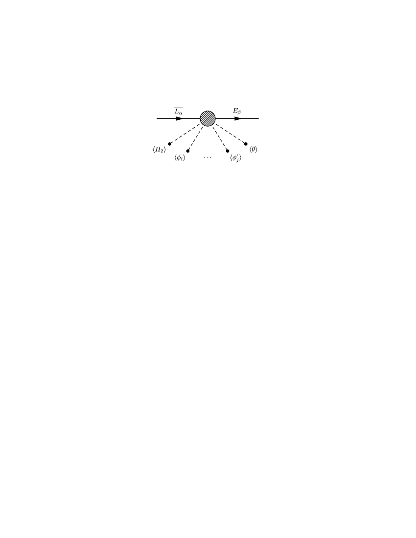
Figure 2: Non-renormalizable terms generating the effective Yukawa couplings in the matrix ${(\mathcal{O}}^{\ell}_{\alpha\beta})$.

We will denote the total number of times that the fields $\phi_{1},\phi_{2},\ldots,\phi_{6}$ appear in the operator ${\mathscr{O}}^{\ell}_{\alpha\beta}$ by $n_{1}$ and the total number of times that their complex conjugates $\phi_{1}^{\dagger},\phi_{2}^{\dagger},\ldots,\phi_{6}^{\dagger}$ appear in the operator ${\mathscr{O}}^{\ell}_{\alpha\beta}$ by $n_{2}$. Now, invariance under transformation of the discrete symmetry ${\mathcal{D}}_{1}$ implies that for the first column of the Yukawa interaction matrix $({\mathscr{O}}^{\ell}_{\alpha\beta})$, i.e., for $\beta=e$, it must hold that $n_{1}-n_{2}=4$. For the second and third column of the Yukawa interaction matrix, i.e., for $\beta=\mu,\tau$, the discrete symmetry ${\mathcal{D}}_{1}$ instead requires that $n_{1}-n_{2}=1$. In addition, we conclude from the transformation properties of the fundamental Froggatt–Nielsen states under the discrete symmetry ${\mathcal{D}}_{6}$ that the operators ${\mathscr{O}}^{\ell}_{\alpha\mu}$ and ${\mathscr{O}}^{\ell}_{\alpha\tau}$, where $\alpha=e,\mu,\tau$, can neither involve the field $\phi_{9}$ nor the field $\phi_{10}$. This is, however, not true for the operators ${\mathscr{O}}^{\ell}_{\alpha e}$ ($\alpha=e,\mu,\tau$) in the first column of the effective Yukawa coupling matrix.

4.1 The first row and column of the charged lepton mass matrix

Invariance under transformations of the U(1) symmetries requires the U(1) charges of the entries ${\mathscr{O}}^{\ell}_{e\mu}$ and ${\mathscr{O}}^{\ell}_{e\tau}$ in the first row of the effective Yukawa coupling matrix $({\mathscr{O}}^{\ell}_{\alpha\beta})$ to be $(1,-1,0)$. Since the fields $\phi_{9}$ and $\phi_{10}$ cannot be involved in the generation of the $e$-$\mu$- and $e$-$\tau$-elements of the charged lepton mass matrix, the U(1) charge assignment immediately implies that any mass operator giving rise to these $e$-$\mu$- and $e$-$\tau$-elements must involve the term $\sim\phi_{1,2}\theta^{2}/(M_{1})^{3}$. Next, the symmetries ${\mathcal{D}}_{5}$ and ${\mathcal{D}}_{6}$ yield to leading order for the operators ${\mathscr{O}}^{\ell}_{e\mu}$ and ${\mathscr{O}}^{\ell}_{e\tau}$ the two possible terms $\sim\phi_{1}\phi_{1}^{\prime}\theta^{2}/(M_{1})^{4}$ and $\sim\phi_{2}\phi_{2}^{\prime}\theta^{2}/(M_{1})^{4}$. In conjuction with the requirement $n_{1}-n_{2}=1$, the symmetry ${\mathcal{D}}_{6}$ implies that any further operators contributing to the operator ${\mathscr{O}}^{\ell}_{e\mu}$ or ${\mathscr{O}}^{\ell}_{e\tau}$ must have at least two powers of mass dimension more than the terms $\phi_{1}\phi_{1}^{\prime}\theta^{2}/(M_{1})^{4}$ and $\phi_{2}\phi_{2}^{\prime}\theta^{2}/(M_{1})^{4}$. We will therefore neglect these additional operators.

From the transformation properties of the right-handed electron $E_{e}$ and the fundamental Froggatt–Nielsen states under transformations of the discrete symmetries ${\mathcal{D}}_{1}$ and ${\mathcal{D}}_{6}$, we conclude that the operators ${\mathscr{O}}^{\ell}_{ee},{\mathscr{O}}^{\ell}_{\mu e}$, and ${\mathscr{O}}^{\ell}_{\tau e}$ in the first column of the effective Yukawa coupling matrix must involve at least a four-fold product of fields taken from the set $\{\phi_{1},\phi_{2},\phi_{3},\phi_{4},\phi_{5},\phi_{6}\}$ times a field taken from the set $\{\phi_{9},\phi_{10}\}$. Possible lowest-dimensional contributions to the operator ${\mathscr{O}}^{\ell}_{ee}$, which are consistent with the symmetries of our model, are, e.g., given by $\sim\phi_{10}\left[(\phi_{3})^{4}+(\phi_{4})^{4}\right]/(M_{1})^{5}$ and $\sim\phi_{10}(\phi_{3})^{2}(\phi_{4})^{2}/(M_{1})^{5}$. For brevity, we will take the operator

$${\mathscr{O}}^{\ell}_{ee}=\frac{\phi_{10}}{(M_{1})^{5}}\left[(\phi_{3})^{4}+(\phi_{4})^{4}\right]$$ (35)

as a representative of these contributions. The remaining operators ${\mathscr{O}}^{\ell}_{\mu e}$ and ${\mathscr{O}}^{\ell}_{\tau e}$ have a mass dimension that is greater than or equal to the mass dimension of the terms in Eq. (35). However, the effects of these terms on the leptonic mixing angles will turn out to be negligible in comparison with the contributions coming from other entries of the charged lepton mass matrix.

In total, the first row of the effective Yukawa coupling matrix of the charged leptons, which is consistent with all of the discrete symmetries, is to leading order

$$({\mathscr{O}}^{\ell}_{e\alpha})=\left(\begin{matrix}A_{1}\left[(\phi_{3})^{4}+(\phi_{4})^{4}\right]\quad&\;B_{1}\left[\phi_{1}\phi_{1}^{\prime}-\phi_{2}\phi_{2}^{\prime}\right]\quad&\;B_{1}\left[\phi_{1}\phi_{1}^{\prime}+\phi_{2}\phi_{2}^{\prime}\right]\end{matrix}\right).$$ (36a)

Here the dimensionful coefficients $$A_{1} B_{1}$$ and are given by

$$A_{1} = Y^{\ell}_{a}\frac{\phi_{10}}{(M_{1})^{5}},$$ (36b)

$$B_{1} = Y^{\ell}_{b}\frac{\theta^{2}}{(M_{1})^{4}},$$ (36c)

where the quantities $Y^{\ell}_{a}$ and $Y^{\ell}_{b}$ are arbitrary order unity coefficients and $M_{1}$ is the high mass scale of the intermediate Froggatt–Nielsen states. Note that at the level of the fundamental theory, the permutation symmetry $\mathcal{D}_{4}$, which interchanges the second and third generations of the leptons, is also propagated to the heavy Froggatt–Nielsen states. This establishes a degeneracy of the associated Yukawa couplings and the explicit masses of these states, which is then translated into a degeneracy of the corresponding effective Yukawa couplings of the low-energy theory.

4.2 The 2-3-submatrix of the charged lepton mass matrix

In the 2-3-submatrix of the charged lepton mass matrix, the U(1) charges of the operators ${\mathscr{O}}^{\ell}_{\alpha\beta}$ ($\alpha,\beta=\mu,\tau$) must be $(0,0,0)$. The lowest dimensional operators which fulfill this condition as well as the constraint $n_{1}-n_{2}=1$ are proportional to $\phi_{3,4}/M_{1}$ or $\phi_{5,6}\theta/(M_{1})^{2}$. Furthermore, invariance under transformation of the discrete symmetries ${\mathcal{D}}_{5}$ and ${\mathcal{D}}_{6}$ implies that the lowest dimensional operators ${\mathscr{O}}_{\alpha\beta}^{\ell}$ in the 2-3-submatrix with $n_{1}-n_{2}=1$ are of the types

$$\frac{\phi_{3}^{\prime}\phi_{3}}{(M_{1})^{2}},\quad\frac{\phi_{4}^{\prime}\phi_{4}}{(M_{1})^{2}},\quad\frac{\phi_{5}^{\prime}\phi_{5}\theta}{(M_{1})^{3}},\quad\frac{\phi_{6}^{\prime}\phi_{6}\theta}{(M_{1})^{3}}.$$ (37)

Thus, the most general 2-3-submatrix of the matrix $({\mathscr{O}}^{\ell}_{\alpha\beta})$, which involves only these combinations and is invariant under transformations of the remaining discrete symmetries, is found to be

$$\left(\begin{matrix}C(\phi_{3}^{\prime}\phi_{3}-\phi_{4}^{\prime}\phi_{4})+D(\phi_{5}^{\prime}\phi_{5}-\phi_{6}^{\prime}\phi_{6})&0\\ 0&C(\phi_{3}^{\prime}\phi_{3}+\phi_{4}^{\prime}\phi_{4})+D(\phi_{5}^{\prime}\phi_{5}+\phi_{6}^{\prime}\phi_{6})\end{matrix}\right).$$ (38a)

Here the dimensionful coefficients $$C D$$ and are given by

$$C = Y^{\ell}_{c}\frac{1}{(M_{1})^{2}},$$ (38b)

$$D = Y^{\ell}_{d}\frac{\theta}{(M_{1})^{3}},$$ (38c)

where the quantities $Y^{\ell}_{c}$ and $Y^{\ell}_{d}$ are arbitrary order unity coefficients. Actually, contributions to the next-leading operators ${\mathscr{O}}^{\ell}_{\mu\tau}$ and ${\mathscr{O}}^{\ell}_{\tau\mu}$ are, e.g., given by

$$\mu \tau : \quad\frac{1}{(M_{1})^{4}}(a_{1}\phi_{7}\phi_{8}^{\dagger}+a_{2}\phi_{8}\phi_{7}^{\dagger})(\phi_{3}+\phi_{4})\phi_{3}^{\prime},$$- (39a)

$$\tau \mu : \quad\frac{1}{(M_{1})^{4}}(a_{2}\phi_{7}\phi_{8}^{\dagger}+a_{1}\phi_{8}\phi_{7}^{\dagger})(\phi_{3}-\phi_{4})\phi_{3}^{\prime},$$- (39b)

where $a_{1}$ and $a_{2}$ are some complex-valued constants. Note that the terms in Eqs. (39) carry only one unit of mass dimension more than, e.g., the term $\phi_{5}^{\prime}\phi_{5}\theta/(M_{1})^{3}$ in Eq. (38a). When diagonalizing the mass matrix, however, it will turn out that the associated corrections to the leptonic mixing parameters and the lepton masses are in fact negligible.

4.3 The charged lepton mass matrix

Combining the results of Secs. 4.1 and 4.2, the leading order effective Yukawa coupling matrix of the charged leptons is

$${\tiny(\mathscr{O}^{\ell}_{\alpha\beta})=\left(\begin{matrix}A_{1}\left[(\phi_{3})^{4}+(\phi_{4})^{4}\right]&B_{1}\left[\phi_{1}\phi_{1}^{\prime}-\phi_{2}\phi_{2}^{\prime}\right]&B_{1}\left[\phi_{1}\phi_{1}^{\prime}+\phi_{2}\phi_{2}^{\prime}\right]\\ 0&C(\phi_{3}^{\prime}\phi_{3}-\phi_{4}^{\prime}\phi_{4})+D(\phi_{5}^{\prime}\phi_{5}-\phi_{6}^{\prime}\phi_{6})&0\\ 0&0&C(\phi_{3}^{\prime}\phi_{3}+\phi_{4}^{\prime}\phi_{4})+D(\phi_{5}^{\prime}\phi_{5}+\phi_{6}^{\prime}\phi_{6})\end{matrix}\right),}$$ (40)

where the dimensionful couplings $A_{1}$, $B_{1}$, $C$, and $D$ are given in Eqs. (36b), (36c), (38b), and (38c), respectively. Inserting the VEVs in Eqs. (29) and (22) into the corresponding operators of the matrix $(\mathscr{O}^{\ell}_{\alpha\beta})$, we observe that, due to the vacuum alignment mechanism of the SM singlet scalar fields, in some of the entries of the matrix $((M_{\ell})_{\alpha\beta}$), the spontaneously generated effective mass terms of a given order exactly cancel, whereas in other entries they do not. Furthermore, the vacuum alignment mechanism correlates these cancellations in the different entries of the matrix $((M_{\ell})_{\alpha\beta})$ in such a way that after SSB the charged lepton mass matrix $M_{\ell}$ can be of the two possible asymmetric forms

$$M_{\ell}\simeq m_{\tau}^{\rm exp}\left(\begin{matrix}\epsilon^{3}&\epsilon^{2}&\epsilon^{4}\\ \epsilon^{3}&\epsilon&\epsilon^{2}\\ \epsilon^{3}&\epsilon^{2}&1\end{matrix}\right)$$ (41)

and

$$M_{\ell}\simeq m_{\tau}^{\rm exp}\left(\begin{matrix}\epsilon^{3}&\epsilon^{4}&\epsilon^{2}\\ \epsilon^{3}&1&\epsilon^{2}\\ \epsilon^{3}&\epsilon^{2}&\epsilon\end{matrix}\right),$$ (42)

where we have also introduced the appropriate orders of magnitude for the matrix elements $(M_{\ell})_{\mu e}$ and $(M_{\ell})_{\tau e}$ as well as for the “phenomenological” (in contrast to exact) texture zeros arising in Eqs. (36a) and (38a). Here $m_{\tau}^{\rm exp}$ is the (experimental) tau mass. Note that a permutation of the second and third generations $L_{\mu}\leftrightarrow L_{\tau},\>E_{\mu}\leftrightarrow E_{\tau}$ leads from one solution to another. Let us consider the first one for our remaining discussion.

5 Yukawa interactions of the neutrinos

Consider the effective Yukawa coupling operators ${\mathscr{O}}_{\alpha\beta}^{\nu}$ which generate the entries in the neutrino mass matrix $M_{\nu}$ via the mass terms

$$\mathscr{L}_{Y}^{\nu}=\overline{L^{c}_{\alpha}}\frac{H_{1}^{2}}{M_{2}}{\mathscr{O}}_{\alpha\beta}^{\nu}L_{\beta}+{\rm h.c.},$$ (43)

where $\alpha,\beta=e,\mu,\tau$ and $M_{2}$ is the relevant high mass scale which is responsible for the smallness of the neutrino masses in comparison with the charged lepton masses. Since the SM singlet neutrinos as well as the Higgs doublets are ${\mathcal{D}}_{1}$-singlets, the presence of the fields $\phi_{1},\phi_{2},\ldots,\phi_{6}$ (which transform non-trivially under the discrete symmetry ${\mathcal{D}}_{1}$) in the operators ${\mathscr{O}}^{\nu}_{\alpha\beta}$ is forbidden. Hence, the only scalar fields that can be involved in the leading order operators ${\mathscr{O}}^{\nu}_{\alpha\beta}$ are $\phi_{7},\phi_{8},\phi_{9},\phi_{10}$, and $\theta$.

5.1 Effective Yukawa interactions of the neutrinos

The operators ${\mathscr{O}}^{\nu}_{\mu\mu},{\mathscr{O}}^{\nu}_{\mu\tau},{\mathscr{O}}^{\nu}_{\tau\mu}$, and ${\mathscr{O}}^{\nu}_{\tau\tau}$ must have the U(1) charge structure $(0,-2,0)$. An example of the lowest dimensional operators which achieve this is

$$\sim\frac{\phi_{9}\phi_{10}\theta}{(M_{1})^{5}}\left[(\phi_{7}^{\dagger})^{2}+(\phi_{8}^{\dagger})^{2}\right].$$ (44)

Since the U(1) charge structure of the entry ${\mathscr{O}}^{\nu}_{ee}$ is $(-2,0,0)$, the operator ${\mathscr{O}}^{\nu}_{ee}$ is to leading order

$${\mathscr{O}}^{\nu}_{ee}=Y_{a}^{\nu}\frac{\phi_{9}\phi_{10}\theta}{(M_{1})^{3}},$$ (45)

where $Y_{a}^{\nu}$ is an arbitrary order unity coefficient. Note that the operators of the type in Eq. (44) carry two units of mass dimension more than the operator ${\mathscr{O}}^{\nu}_{ee}$.

The operators ${\mathscr{O}}^{\nu}_{e\mu}$ and ${\mathscr{O}}^{\nu}_{e\tau}$ (as well as ${\mathscr{O}}^{\nu}_{\mu e}$ and ${\mathscr{O}}^{\nu}_{\tau e}$) must have the U(1) charge structure $(-1,-1,0)$. Therefore, the lowest dimensional terms which contribute to these operators are $\sim\phi_{7}/M_{1}$ and $\sim\phi_{8}/M_{1}$. The symmetries ${\mathcal{D}}_{2},{\mathcal{D}}_{3}$, and ${\mathcal{D}}_{4}$ then yield to leading order ${\mathscr{O}}_{e\mu}^{\nu}=Y_{b}^{\nu}\phi_{7}/M_{1}$ and ${\mathscr{O}}_{e\tau}^{\nu}=Y_{b}^{\nu}\phi_{8}/M_{1}$, where $Y_{b}^{\nu}$ is an arbitrary order unity coefficient. Note that the operator ${\mathscr{O}}^{\nu}_{ee}$ in Eq. (45) carries two units of mass dimension more than the operators ${\mathscr{O}}_{e\mu}^{\nu}\sim\phi_{7}/M_{1}$ and ${\mathscr{O}}_{e\tau}^{\nu}\sim\phi_{8}/M_{1}$. We will therefore not in detail consider the structure of the highly suppressed terms that appear in the 2-3-submatrix of the neutrino mass matrix as the operator given in Eq. (44).

In total, the most general effective Yukawa coupling matrix of the neutrinos $({\mathscr{O}}_{\alpha\beta}^{\nu})$ that is consistent with the symmetries of our model is to leading order given by

$$({\mathscr{O}}^{\nu}_{\alpha\beta})=\left(\begin{matrix}A_{2}&B_{2}&B_{3}\\ B_{2}&0&0\\ B_{3}&0&0\end{matrix}\right).$$ (46)

Here the dimensionful coefficients $A_{2}$, $B_{2}$, and $B_{3}$ are given by

$$A_{2} = Y_{a}^{\nu}\frac{\phi_{9}\phi_{10}\theta}{(M_{1})^{3}},$$ (47a)

$$B_{2} = Y_{b}^{\nu}\frac{\phi_{7}}{M_{1}},$$ (47b)

$$B_{3} = Y_{b}^{\nu}\frac{\phi_{8}}{M_{1}},$$ (47c)

where the quantity $Y^{\nu}_{b}$ is an order unity coefficient. The leading order tree level realizations of the higher-dimensional operators, which generate the neutrino masses, are shown in Figs. 3 and 4.

Figure 3: The dimension six operator for $\alpha=\mu,\tau$ and $\phi_{\mu}\equiv\phi_{7}$, $\phi_{\tau}\equiv\phi_{8}$ generating the $e$-$\mu$- and $e$-$\tau$-elements in the effective neutrino mass matrix.

Figure 4: The dimension eight operators generating the $e$-$e$-element in the effective neutrino mass matrix.

Note that the coefficients $B_{2}$ and $B_{3}$ contain the same Yukawa coupling constant $Y^{\nu}_{b}$. Furthermore, we point out that the texture zeros in the 2-3-submatrix of the effective neutrino Yukawa matrix should be understood as “phenomenological” ones, since they actually represent highly suppressed operators carrying two units of mass dimension more than the entry ${\mathscr{O}}^{\nu}_{ee}$.

5.2 The neutrino mass matrix

Inserting the VEVs in Eq. (12) into the effective operators in Eqs. (47), we obtain from Eq. (46) the effective neutrino mass matrix (to leading order)

$$M_{\nu}=\frac{\langle H_{1}\rangle^{2}}{M_{2}}\left(\begin{matrix}Y_{a}^{\nu}\epsilon^{3}&Y_{b}^{\nu}\epsilon&\pm Y_{b}^{\nu}\epsilon\\ Y_{b}^{\nu}\epsilon&\epsilon^{5}&\epsilon^{5}\\ \pm Y_{b}^{\nu}\epsilon&\epsilon^{5}&\epsilon^{5}\\ \end{matrix}\right),$$ (48)

where we have introduced the actual orders of magnitude of the higher-order corrections to the texture zeros in the 2-3-submatrix of the matrix in Eq. (46). Note that after SSB the symmetries determine the $e$-$\mu$- and $e$-$\tau$-elements to be exactly degenerate (up to a sign), giving rise to an atmospheric mixing angle which is close to maximal (higher-order corrections to exact maximal atmospheric mixing mainly come from the $\mu$-$\tau$- and $\tau$-$\mu$-elements of the charged lepton mass matrix). Introducing an “absolute” neutrino mass scale $m_{\nu}$ and choosing $Y^{\nu}_{a}/Y^{\nu}_{b}\simeq 1$, we can write the neutrino mass matrix in Eq. (48) as

$$M_{\nu}\simeq m_{\nu}\left(\begin{matrix}\epsilon^{2}&1&-1\\ 1&\epsilon^{4}&\epsilon^{4}\\ -1&\epsilon^{4}&\epsilon^{4}\end{matrix}\right),$$ (49)

where

$$m_{\nu}=\frac{\langle H_{1}\rangle^{2}}{M_{2}}Y^{\nu}_{b}\epsilon.$$ (50)

Note that we have chosen the minus signs for the $e$-$\tau$- and $\tau$-$e$-elements due to our freedom of absorbing the corresponding phase into the order unity coefficients in the charged lepton sector. Furthermore, it is important to keep in mind that the entries “1” and “$-1$” of the matrix in Eq. (49) indeed denote matrix elements, which are degenerate to a very high accuracy, whereas the other entries are only known up to their order unity coefficients.

6 Lepton masses and leptonic mixings

From the results of the last two sections we have seen that the lepton mass matrices are given by

$$M_{\ell}\simeq m_{\tau}^{\rm exp}\left(\begin{matrix}\epsilon^{3}&\epsilon^{2}&\epsilon^{4}\\ \epsilon^{3}&\epsilon&\epsilon^{2}\\ \epsilon^{3}&\epsilon^{2}&1\end{matrix}\right)\quad\mbox{and}\quad M_{\nu}\simeq m_{\nu}\left(\begin{matrix}\epsilon^{2}&1&-1\\ 1&\epsilon^{4}&\epsilon^{4}\\ -1&\epsilon^{4}&\epsilon^{4}\end{matrix}\right),$$

where again $m_{\tau}^{\rm exp}$ is the (experimental) tau mass, $m_{\nu}$ is some “absolute” neutrino mass scale, $\epsilon\simeq 0.1$ is the small expansion parameter (defined in Sec. 3), and only the order of magnitude of the matrix elements have been indicated. In the above expression, the first matrix is the charged lepton mass matrix and the second matrix is the neutrino mass matrix. Note that the small expansion parameter $\epsilon$ is the same for both matrices. In order to find the leptonic mixing angles and the lepton masses, we have to perform diagonalizations of the above two displayed mass matrices. Let us begin with the diagonalization of the charged lepton mass matrix. Since this matrix is not symmetric and we want to extract the relevant mass and mixing parameters, we have, in fact, to diagonalize the matrix product $M_{\ell}M_{\ell}^{\dagger}$, which is a symmetric matrix. Biunitary diagonalization of the matrix $M_{\ell}$ implies that $U_{\ell}^{\dagger}M_{\ell}V_{\ell}=\mathcal{M}_{\ell}$, where $\mathcal{M}_{\ell}={\rm diag\,}(m_{e},m_{\mu},m_{\tau})$ is the diagonalized charged lepton mass matrix containing the masses of the charged leptons (i.e., the eigenvalues of the matrix $\sqrt{M_{\ell}M_{\ell}^{\dagger}}$) and $U_{\ell}$ and $V_{\ell}$ are two unitary mixing matrices. Thus, we obtain $\mathcal{M}_{\ell}\mathcal{M}_{\ell}^{\dagger}=U_{\ell}^{\dagger}M_{\ell}M_{\ell}^{\dagger}U_{\ell}$, where $U_{\ell}$ will be the charged lepton mixing matrix. Note that the mixing matrix $V_{\ell}$ does not appear in the diagonalization of the matrix product $M_{\ell}M_{\ell}^{\dagger}$. Actually, since the matrix $M_{\ell}$ is a real matrix, we have $\mathcal{M}_{\ell}\mathcal{M}_{\ell}^{\dagger}=\mathcal{M}_{\ell}\mathcal{M}_{\ell}^{T}=U_{\ell}^{T}M_{\ell}M_{\ell}^{T}U_{\ell}$. Next, straight-forward calculations (using App. A) yield

$$\mathcal{M}_{\ell}\mathcal{M}_{\ell}^{\dagger}=(m_{\tau}^{\rm exp})^{2}\;{\rm diag\,}(\epsilon^{6}-2\epsilon^{7}+\mathcal{O}(\epsilon^{9}),\epsilon^{2}+\epsilon^{4}+\mathcal{O}(\epsilon^{5}),1+2\epsilon^{4}+\mathcal{O}(\epsilon^{5}))$$ (51)

and

$$U_{\ell}\equiv((U_{\ell})_{\alpha a})\simeq\left(\begin{matrix}-0.995&-0.0997&-0.000212\\ 0.0997&-0.995&-0.0111\\ -0.000897&0.0111&-1.000\end{matrix}\right)$$ (52)

such that $U_{\ell}^{\dagger}U_{\ell}\simeq U_{\ell}U_{\ell}^{\dagger}\simeq 1_{3}$, where $\alpha=e,\mu,\tau$ and $a=1,2,3$. Note that the charged lepton mixing matrix $U_{\ell}$ is independent of the absolute charged lepton mass scale $m_{\tau}^{\rm exp}$, i.e., the tau mass. This means that the charged lepton (and, of course, the leptonic) mixing angles will not depend on the tau mass. The charged lepton masses are given as the square roots of (the absolute values of) the eigenvalues of the matrix product $M_{\ell}M_{\ell}^{\dagger}$, i.e., $m_{e}=m_{\tau}^{\rm exp}\epsilon^{3}\left(1-\epsilon+\mathcal{O}(\epsilon^{2})\right)$, $m_{\mu}=m_{\tau}^{\rm exp}\epsilon\left(1+\tfrac{1}{2}\epsilon^{2}+\mathcal{O}(\epsilon^{3})\right)$, and $m_{\tau}=m_{\tau}^{\rm exp}\left(1+\epsilon^{4}+\mathcal{O}(\epsilon^{5})\right)$. Thus, the order-of-magnitude relations for the charged lepton masses are given by

$$m_{e}/m_{\mu}\simeq\epsilon^{2}\simeq 10^{-2}\quad\mbox{and}\quad m_{\mu}/m_{\tau}\simeq\epsilon\simeq 10^{-1},$$ (53)

which approximately fit the experimentally observed values, i.e., $(m_{e}/m_{\mu})_{\rm exp}\simeq 4.8\cdot 10^{-3}$ and $(m_{\mu}/m_{\tau})_{\rm exp}\simeq 5.9\cdot 10^{-2}$ [28]. Furthermore, the charged lepton mixing angles (in the “standard” parameterization) are found to be (using App. A) [69, 70, 49]

$$\theta_{12}^{\ell} \equiv \arctan\left|\frac{(U_{\ell})_{e2}}{(U_{\ell})_{e1}}\right|=\epsilon-\frac{1}{3}\epsilon^{3}+\mathcal{O}(\epsilon^{4}),$$ (54)

$$\theta_{13}^{\ell} \equiv \arcsin|(U_{\ell})_{e3}|=2\epsilon^{2}+\epsilon^{5}+\mathcal{O}(\epsilon^{6}),$$ (55)

$$\theta_{23}^{\ell} \equiv \arctan\left|\frac{(U_{\ell})_{\mu 3}}{(U_{\ell})_{\tau 3}}\right|=\epsilon^{2}+\epsilon^{3}+\mathcal{O}(\epsilon^{4}).$$ (56)

Inserting $\epsilon\simeq 0.1$ into Eqs. (54) - (56), we obtain $\theta_{12}^{\ell}\simeq 5.72^{\circ}\approx 6^{\circ}$, $\theta_{13}^{\ell}\simeq 0.0122^{\circ}\approx 0.01^{\circ}$, and $\theta_{23}^{\ell}\simeq 0.637^{\circ}\approx 0.6^{\circ}$, i.e., the mixing angles in the charged lepton sector are all small. The mixing angle $\theta^{\ell}_{12}$ is the only one that is not negligible. Thus, it will finally yield a non-zero contribution to the leptonic mixing angles [49].

Next, we want to diagonalize the neutrino mass matrix $M_{\nu}$. The diagonalization procedure of the matrix $M_{\nu}$ is easier than the one of the matrix $M_{\ell}$, since the matrix $M_{\nu}$ is a symmetric matrix. Diagonalization of the matrix $M_{\nu}$ directly implies that $U_{\nu}^{T}M_{\nu}U_{\nu}=\mathcal{M}_{\nu}$, where $\mathcal{M}_{\nu}={\rm diag\,}(m_{\nu_{1}},m_{\nu_{2}},m_{\nu_{3}})$ is the diagonalized neutrino mass matrix containing the masses of the neutrino mass eigenstates (i.e., the eigenvalues of the matrix $M_{\nu}$) and $U_{\nu}$ is the unitary neutrino mixing matrix. Straight-forward calculations (using App. A) yield

$$\mathcal{M}_{\nu} = m_{\nu}\;{\rm diag\,}\left(\frac{1}{2}\left(\epsilon^{2}+\sqrt{8+\epsilon^{4}}\right),\frac{1}{2}\left(\epsilon^{2}-\sqrt{8+\epsilon^{4}}\right),2\epsilon^{4}\right)$$

$$= m_{\nu}\;{\rm diag\,}\left(\sqrt{2}+\frac{1}{2}\epsilon^{2}+\frac{1}{8\sqrt{2}}\epsilon^{4}+\mathcal{O}(\epsilon^{8}),-\sqrt{2}+\frac{1}{2}\epsilon^{2}-\frac{1}{8\sqrt{2}}\epsilon^{4}+\mathcal{O}(\epsilon^{8}),2\epsilon^{4}\right)$$

and

$$U_{\nu}\equiv((U_{\nu})_{\alpha a})\simeq\left(\begin{matrix}0.708&0.706&0\\ 0.499&-0.501&\frac{1}{\sqrt{2}}\\ -0.499&0.501&\frac{1}{\sqrt{2}}\end{matrix}\right)$$ (58)

such that $U_{\nu}^{\dagger}U_{\nu}\simeq U_{\nu}U_{\nu}^{\dagger}\simeq 1_{3}$, where $\alpha=e,\mu,\tau$ and $a=1,2,3$. Note that the neutrino mixing matrix $U_{\nu}$ is independent of the absolute neutrino mass scale $m_{\nu}$. This means that the neutrino (and, of course, the leptonic) mixing angles will not depend on this scale. The (physical) neutrino masses are given as (the absolute values of) the eigenvalues of the neutrino mass matrix $M_{\nu}$, i.e., $m_{1}\equiv|m_{\nu_{1}}|\simeq\sqrt{2}m_{\nu}$, $m_{2}\equiv|m_{\nu_{2}}|\simeq\sqrt{2}m_{\nu}$, and $m_{3}\equiv|m_{\nu_{3}}|=2\epsilon^{4}m_{\nu}\approx 0$, which means that we have an inverted neutrino mass hierarchy spectrum (i.e., $m_{3}\ll m_{1}\simeq m_{2}\quad\Rightarrow\quad 0\simeq|\Delta m_{21}^{2}|\ll|\Delta m_{32}^{2}|\simeq|\Delta m_{31}^{2}|$). Naturally, the neutrino mass squared differences $\Delta m_{ab}^{2}\equiv m_{\nu_{a}}^{2}-m_{\nu_{b}}^{2}=m_{a}^{2}-m_{b}^{2}$, where $m_{\nu_{a}}$ is the mass and $m_{a}$ is the physical mass of the $a$th neutrino mass eigenstate, respectively, are given as follows:

$$\Delta m_{21}^{2} = m_{\nu}^{2}\left(-2\sqrt{2}\epsilon^{2}-\frac{1}{4\sqrt{2}}\epsilon^{6}+\mathcal{O}(\epsilon^{10})\right),$$ (59)

$$\Delta m_{32}^{2} = m_{\nu}^{2}\left(-2+\sqrt{2}\epsilon^{2}-\frac{1}{2}\epsilon^{4}+\mathcal{O}(\epsilon^{6})\right),$$ (60)

$$\Delta m_{31}^{2} = m_{\nu}^{2}\left(-2-\sqrt{2}\epsilon^{2}-\frac{1}{2}\epsilon^{4}+\mathcal{O}(\epsilon^{6})\right).$$ (61)

Note that the leading order terms in Eqs. (59) - (61) are all negative, which is natural, since we have an inverted mass hierarchy spectrum for the neutrinos. Hence, the solar and atmospheric neutrino mass squared differences are given by $\Delta m_{\odot}^{2}\equiv|\Delta m_{21}^{2}|\simeq 2\sqrt{2}\epsilon^{2}m_{\nu}^{2}$ and $\Delta m_{\rm atm}^{2}\equiv|\Delta m_{32}^{2}|\simeq|\Delta m_{31}^{2}|\simeq 2m_{\nu}^{2}$, respectively. The “experimental” values of these quantities are $\Delta m_{\odot}^{2}\simeq 5.0\cdot 10^{-5}\,{\rm eV}^{2}$ [23] and $\Delta m_{\rm atm}^{2}\simeq 2.5\cdot 10^{-3}\,{\rm eV}^{2}$ [8]. Thus, we extract that $m_{\nu}\simeq 0.04\,{\rm eV}$ and $\epsilon\simeq 0.1$, which is consistent and agrees perfectly with our used value for the small expansion parameter $\epsilon$. In other words, using $\epsilon\simeq 0.1$ and $m_{\nu}\simeq 0.04\,{\rm eV}$ for the absolute neutrino mass scale (Nobody knows where this value comes from!), we obtain the presently preferred values for the solar and atmospheric neutrino mass squared differences. Furthermore, we have that $m_{1}\simeq m_{2}\simeq 0.05\,{\rm eV}$ and $m_{3}\simeq 1\cdot 10^{-5}\,{\rm eV}\approx 0$. Similarly, as for the charged leptons, the neutrino mixing angles (in the “standard” parameterization) are found to be (using App. A) [69, 70, 49]

$$\theta_{12}^{\nu} \equiv \arctan\left|\frac{(U_{\nu})_{e2}}{(U_{\nu})_{e1}}\right|=\frac{\pi}{4}+\frac{1}{4\sqrt{2}}\epsilon^{2}-\frac{1}{96\sqrt{2}}\epsilon^{6}+\mathcal{O}(\epsilon^{10}),$$ (62)

$$\theta_{13}^{\nu} \equiv \arcsin|(U_{\nu})_{e3}|=0,$$ (63)

$$\theta_{23}^{\nu} \equiv \arctan\left|\frac{(U_{\nu})_{\mu 3}}{(U_{\nu})_{\tau 3}}\right|=\frac{\pi}{4}.$$ (64)

Inserting $\epsilon\simeq 0.1$ into Eqs. (62) - (64), we obtain $\theta_{12}^{\nu}\simeq 45.1^{\circ}\approx 45^{\circ}$, $\theta_{13}^{\nu}=0$, and $\theta_{23}^{\nu}=45^{\circ}$, which means that we have (nearly) bimaximal mixing in the neutrino sector. Note that the values for $\theta_{13}^{\nu}$ and $\theta_{23}^{\nu}$ are exact, since they are only determined from the matrix elements of the third column of the matrix $U_{\nu}$ in Eq. (58).

7 The leptonic mixing angles

The leptonic mixing angles (or parameters if one also includes the $\mathcal{CP}$ violation phase $\delta$) are given by the leptonic mixing matrix. The leptonic mixing matrix $U$ is composed of the charged lepton mixing matrix $U_{\ell}$ and the neutrino mixing matrix $U_{\nu}$ as follows:

$$U\equiv U_{\ell}^{\dagger}U_{\nu}.$$ (65)

The matrix $U_{\ell}$ ($U_{\nu}$) rotates the left-handed charged lepton fields (the neutrino fields) so that the charged lepton mass matrix $M_{\ell}$ (the neutrino mass matrix $M_{\nu}$) becomes diagonal (see Sec. 6), i.e., it relates the flavor state and mass eigenstate bases. Thus, one can look upon the matrix $U$ [$U_{ab}=(U_{\ell}^{\dagger}U_{\nu})_{ab}=\sum_{\alpha=e,\mu,\tau}(U_{\ell}^{\dagger})_{a\alpha}(U_{\nu})_{\alpha b}=\sum_{\alpha=e,\mu,\tau}(U_{\ell})^{\ast}_{\alpha a}(U_{\nu})_{\alpha b}$] as the messenger between the mass eigenstate bases of the charged leptons and the neutrinos. Inserting the matrices in Eqs. (52) and (58) into the definition in Eq. (65), we find that

$$U\equiv(U_{ab})\simeq\left(\begin{matrix}-0.655&-0.753&0.0699\\ -0.573&0.434&-0.696\\ 0.493&-0.495&-0.715\end{matrix}\right),$$ (66)

which fulfill the condition $U^{\dagger}U=UU^{\dagger}=1_{3}$ to a very good accuracy. Now, the leptonic mixing angles (in the “standard” parameterization [see App. A]) can be read off as follows [69, 70, 49]:

$$\theta_{12} \equiv \arctan\left|\frac{U_{12}}{U_{11}}\right|,$$ (67)

$$\theta_{13} \equiv \arcsin|U_{13}|,$$ (68)

$$\theta_{23} \equiv \arctan\left|\frac{U_{23}}{U_{33}}\right|.$$ (69)

Thus, inserting the appropriate matrix elements of the matrix $U$ expressed in terms of the small expansion parameter $\epsilon$ ($\epsilon\ll 1$) in Eq. (65) into Eqs. (67) - (69), we obtain

$$\theta_{12} = \frac{\pi}{4}-\frac{1}{\sqrt{2}}\epsilon+\frac{1}{4\sqrt{2}}\epsilon^{2}+\mathcal{O}(\epsilon^{3}),$$ (70)

$$\theta_{13} = \frac{1}{\sqrt{2}}\epsilon-\frac{17}{12\sqrt{2}}\epsilon^{3}+\mathcal{O}(\epsilon^{4}),$$ (71)

$$\theta_{23} = \frac{\pi}{4}-\frac{5}{4}\epsilon^{2}-\epsilon^{3}+\mathcal{O}(\epsilon^{4}).$$ (72)

Note that the first correction to the atmospheric (neutrino) mixing angle $\theta_{23}$ is of second order in the small expansion parameter $\epsilon$, and it is therefore very small, i.e., the atmospheric mixing angle stays nearly maximal, $\theta_{23}\simeq\tfrac{\pi}{4}$. However, the first corrections to the solar (neutrino) mixing angle $\theta_{12}$ and the reactor (neutrino) mixing angle (the so-called CHOOZ mixing angle) $\theta_{13}$ are both of first order in the small expansion parameter $\epsilon$ and they are of exactly the same size, but with opposite sign. Thus, we have the first order relation $\theta_{12}\simeq\tfrac{\pi}{4}-\theta_{13}$. Finally, inserting $\epsilon\simeq 0.1$ in Eqs. (70) - (72), we find that the leptonic mixing angles are

$$\theta_{12}\simeq 41.0^{\circ}\approx 41^{\circ},\quad\theta_{13}\simeq 4.01^{\circ}\approx 4^{\circ},\quad\mbox{and}\quad\theta_{23}\simeq 44.2^{\circ}\approx 44^{\circ},$$

which means that we have bilarge leptonic mixing. These values of the leptonic mixing angles lie within the ranges preferred by the MSW LMA solution of the solar neutrino problem, atmospheric neutrino data (nearly maximal atmospheric mixing), and CHOOZ reactor neutrino data. The so-called CHOOZ upper bound is $\sin^{2}\theta_{13}\lesssim 0.10$ (i.e., $|\theta_{13}|\lesssim 9.2^{\circ}$) [72, 73, 74]. In particular, the obtained value for the solar mixing angle $\theta_{12}$ implies a significant deviation from maximal solar mixing. However, the solar mixing angle is bounded from below by approximately $41^{\circ}$ and it is therefore still too close to maximal to be in the 90% (or 95% or 99%) confidence level region of the MSW LMA solution [23].

As we have seen the symmetries of our model generate the hierarchical charged lepton mass spectrum as well as an essentially maximal atmospheric mixing angle. However, these symmetries only determine the order of magnitude of the entries $(M_{\ell})_{\alpha\beta}$ in the charged lepton mass matrix $M_{\ell}$. In order to decide whether the model can naturally give the MSW LMA solution or not, we can test the robustness of the above calculated leptonic mixing angles (and charged lepton masses) under variation of the involved order unity coefficients. For example, by changing the ratio of the order unity coefficients $Y_{b}^{\ell}/Y_{d}^{\ell}$ from 1 to 2 leads to

$$\theta_{12}\simeq 37^{\circ},\quad\theta_{13}\simeq 8^{\circ},\quad\mbox{and}\quad\theta_{23}\simeq 44^{\circ},$$

where the new value for $\theta_{12}$ lies within the 90% (and 95% and 99% and 99.73%) confidence level region of the MSW LMA solution [23] and the new value for $\theta_{13}$ is still below the CHOOZ upper bound. Note that the new values for $\theta_{23}$ is, in principle, the same as the old one. At the same time, the exact values of the charged lepton masses can be accommodated by choosing the values $Y^{\ell}_{a}=0.5$, $Y^{\ell}_{c}=1.8$, and $Y^{\ell}_{d}=1.0$ for the order unity coefficients. Hence, our model is in prefect agreement with the MSW LMA solution and it can reproduce the realistic charged lepton mass spectrum.

8 Implications for neutrinoless double $\beta$-decay, astrophysics, and cosmology

Assuming massive Majorana neutrinos, we analyze the implication for the prediction of the effective Majorana mass $|\langle m\rangle|$ in neutrinoless double $\beta$-decay (see, e.g., Refs.[75, 76])

$$|\langle m\rangle|\equiv\left|\sum_{a=1}^{3}U_{1a}^{2}m_{\nu_{a}}\right|,$$ (73)

where the $U_{1a}$’s are first row matrix elements of the leptonic mixing matrix $U$ and the $m_{\nu_{a}}$’s are the masses of the neutrino mass eigenstates. Inserting the expressions for the $U_{1a}$’s and the $m_{\nu_{a}}$’s into Eq. (73), we obtain

$$|\langle m\rangle| = \frac{1}{2}m_{\nu}\left[\left(\sqrt{8+\epsilon^{4}}\cos 2\theta_{12}+\epsilon^{2}\right)\cos^{2}\theta_{13}+4\epsilon^{4}\sin^{2}\theta_{13}\right]$$ (74)

$$= m_{\nu}\bigg{[}\sqrt{2}\cos 2\theta_{12}\cos^{2}\theta_{13}+\frac{1}{2}\cos^{2}\theta_{13}\epsilon^{2}$$

$$+\left(\frac{1}{8\sqrt{2}}\cos 2\theta_{12}\cos^{2}\theta_{13}+2\sin^{2}\theta_{13}\right)\epsilon^{4}+\mathcal{O}(\epsilon^{8})\bigg{]}$$

$$\simeq m_{\nu}\sqrt{2}\cos 2\theta_{12}\cos^{2}\theta_{13}.$$

Note that the quantity $|\langle m\rangle|$ becomes equal to zero when $\theta_{12}=\tfrac{\pi}{4}$, i.e., when we have an exactly maximal solar mixing angle. Using $m_{\nu}\simeq 0.04\,{\rm eV}$, $\theta_{12}\simeq 41^{\circ}$, and $\theta_{13}\simeq 4^{\circ}$, we find that $|\langle m\rangle|\simeq 0.007\,{\rm eV}$, which is consistent with and below the phenomenological upper bound $|\langle m\rangle|<0.080\,{\rm eV}$ [78] for an inverted hierarchical neutrino mass spectrum. Our value for $|\langle m\rangle|$ is also below the experimental upper bound obtained from neutrinoless double $\beta$-decay experiments (${}^{76}{\rm Ge}$ experiments) by the Heidelberg-Moscow collaboration [$|\langle m\rangle|<0.35\,{\rm eV}$ (@ 90% C.L.)] [79] and by the IGEX collaboration [$|\langle m\rangle|<(0.33\div 1.35)\,{\rm eV}$ (@ 90% C.L.)] [80, 81]. It would also be below the sensitivity of the planned neutrinoless double $\beta$-decay experiments GENIUS, EXO, MAJORANA, and MOON, which is $|\langle m\rangle|\sim 0.01\,{\rm eV}$.

Furthermore, the sum of the neutrino masses

$$M\equiv\sum_{a=1}^{3}m_{a},$$ (75)

where the $m_{a}$’s are the physical masses of the neutrino mass eigenstates, is often used in astrophysics and cosmology. Inserting the expressions for the $m_{a}$’s into Eq. (75), we obtain

$$M = m_{\nu}\left(\sqrt{8+\epsilon^{2}}+2\epsilon^{4}\right)$$ (76)

$$= m_{\nu}\left[2\sqrt{2}+\left(2+\frac{1}{4\sqrt{2}}\right)\epsilon^{4}-\frac{1}{128\sqrt{2}}\epsilon^{8}+\mathcal{O}(\epsilon^{10})\right]\simeq 2\sqrt{2}m_{\nu}.$$

Again using $m_{\nu}\simeq 0.04\,{\rm eV}$, we find that $M\simeq 0.1\,{\rm eV}$. There exist several upper bounds for this quantity from several different branches of astrophysics and cosmology. For example, using the presently best available data from cosmic microwave background radiation and large scale structure measurements, we have the upper bound $M<(2.5\div 3)\,{\rm eV}$ (@ 95% C.L.) [82, 83]. Other upper bounds of this quantity come, e.g., from cosmic microwave background radiation, galaxy clustering, and Lyman Alpha Forest measurements $M<4.2\,{\rm eV}$ (@ 95% C.L.) [84] and from the 2dF Galaxy Redshift Survey $M<(1.8\div 2.2)\,{\rm eV}$ (@ 95% C.L.) [85]. Thus, our value for the sum of neutrino masses is well below the upper bounds derived from astrophysics and cosmology. However, it should be possible to combine cosmic microwave background radiation data from the MAP/Planck satellite with Sloan Digital Sky Survey measurements, which could give an upper bound of $M<0.3\,{\rm eV}$ [86]. Then, our obtained value for the sum of the neutrino masses is rather close to this upper bound.

9 Summary and conclusions

In summary, we have presented a model based on flavor symmetries and higher-dimensional mass operators. This model is a modified and extended version of the model given in Ref.[49] and it naturally yields the mass matrix textures

$$\left(\begin{matrix}\epsilon^{3}&\epsilon^{2}&\epsilon^{4}\\ \epsilon^{3}&\epsilon&\epsilon^{2}\\ \epsilon^{3}&\epsilon^{2}&1\end{matrix}\right)\quad\mbox{and}\quad\left(\begin{matrix}\epsilon^{2}&1&-1\\ 1&\epsilon^{4}&\epsilon^{4}\\ -1&\epsilon^{4}&\epsilon^{4}\end{matrix}\right)$$

for the charged leptons and the neutrinos, respectively. Note that these textures involve the same small expansion parameter $\epsilon$. Our old model [49] had a symmetric mass matrix for the charged leptons, whereas the new model has an asymmetric one. Thus, our new model predicts the realistic charged lepton mass spectrum (with the order unity coefficients $Y^{\ell}_{a}=0.5$, $Y^{\ell}_{c}=1.8$, and $Y^{\ell}_{d}=1.0$), an inverted hierarchical neutrino mass spectrum, a large (but not necessarily close to maximal) solar mixing angle $\theta_{12}$, which is in excellent agreement with the MSW LMA solution of the solar neutrino problem, a small reactor mixing angle $\theta_{13}$, and an approximately maximal atmospheric mixing angle $\theta_{23}$ (enforced by the flavor symmetries). Furthermore, these textures yield the MSW LMA solution and it follows from the model that $\theta_{12}\simeq\tfrac{\pi}{4}-\theta_{13}$. The explicitly obtained values for the mixing angles (assuming no $\mathcal{CP}$ violation, i.e., $\delta=0$) are

$$\theta_{12}\simeq 41^{\circ},\quad\theta_{13}\simeq 4^{\circ},\quad\mbox{and}\quad\theta_{23}\simeq 44^{\circ}$$

for the ratio of the order unity coefficients $Y^{\ell}_{b}/Y^{\ell}_{d}=1$ and

$$\theta_{12}\simeq 37^{\circ},\quad\theta_{13}\simeq 8^{\circ},\quad\mbox{and}\quad\theta_{23}\simeq 44^{\circ},$$

for the ratio of the order unity coefficients $Y^{\ell}_{b}/Y^{\ell}_{d}=2$. Both these sets of the leptonic mixing angles are in very good agreement with present experimental data. In addition, our values are not in conflict with limits coming from neutrinoless double $\beta$-decay, astrophysics, and cosmology.

Finally, we have also (in the Appendix) presented a scheme for how to transform any given $3\times 3$ unitary matrix to the “standard” parameterization form of the Particle Data Group.

Appendix A Transformation of any $3\times 3$ unitary matrix to the “standard” parameterization form

The “standard” parameterization form of a $3\times 3$ unitary matrix according to the Particle Data Group [28] reads

$$U=\left(\begin{matrix}C_{2}C_{3}&S_{3}C_{2}&S_{2}{\rm e}^{-{\rm i}\delta}\\ -S_{3}C_{1}-S_{1}S_{2}C_{3}{\rm e}^{{\rm i}\delta}&C_{1}C_{3}-S_{1}S_{2}S_{3}{\rm e}^{{\rm i}\delta}&S_{1}C_{2}\\ S_{1}S_{3}-S_{2}C_{1}C_{3}{\rm e}^{{\rm i}\delta}&-S_{1}C_{3}-S_{2}S_{3}C_{1}{\rm e}^{{\rm i}\delta}&C_{1}C_{2}\end{matrix}\right),$$ (77)

where $S_{a}\equiv\sin\theta_{a}$, $C_{a}\equiv\cos\theta_{a}$ (for $a=1,2,3$), and $\delta$ is the physical $\mathcal{CP}$ violation phase. Here $\theta_{1}\equiv\theta_{23}$, $\theta_{2}\equiv\theta_{13}$, and $\theta_{3}\equiv\theta_{12}$ are the Euler (mixing) angles. Note that four of the entries of the matrix $U$ in Eq. (77) are real, i.e., the 1-1, 1-2, 2-3, and 3-3 entries. Furthermore, the matrix $U$ in Eq. (77) can be decomposed as follows:

$$U = O_{23}(\theta_{23})U_{13}(\theta_{13},\delta)O_{12}(\theta_{12})$$ (78)

$$= \left(\begin{matrix}1&0&0\\ 0&C_{23}&S_{23}\\ 0&-S_{23}&C_{23}\end{matrix}\right)\left(\begin{matrix}C_{13}&0&S_{13}{\rm e}^{-{\rm i}\delta}\\ 0&1&0\\ -S_{13}{\rm e}^{{\rm i}\delta}&0&C_{13}\end{matrix}\right)\left(\begin{matrix}C_{12}&S_{12}&0\\ -S_{12}&C_{12}&0\\ 0&0&1\end{matrix}\right),$$

where $C_{ab}\equiv\cos\theta_{ab}$, $S_{ab}\equiv\sin\theta_{ab}$ (for $a,b=1,2,3$), and $O_{ab}(\theta_{ab})$ is a rotation by an angle $\theta_{ab}$ in the $ab$-plane. If $\delta=0$, then $U_{13}(\theta_{13},0)=O_{13}(\theta_{13})$.

Here we will show how to transform any given $3\times 3$ unitary matrix to the “standard” parameterization form. A $3\times 3$ unitary matrix

$$U\equiv(U_{ab})=\left(\begin{matrix}U_{11}&U_{12}&U_{13}\\ U_{21}&U_{22}&U_{23}\\ U_{31}&U_{32}&U_{33}\end{matrix}\right)$$ (79)

where $a,b=1,2,3$, obeys $U^{\dagger}U=UU^{\dagger}=1_{3}$ (9 unitarity conditions) and is therefore characterized by 9 real parameters, since a general $3\times 3$ complex matrix is characterized by 18 real parameters (9 complex parameters). Out of these 9 parameters, 3 are Euler (mixing) angles and 6 are phase factors (phases). Not all of the 6 phases enter into expressions for physically measurable quantities. Only those phases are physical, which cannot be eliminated by the transformation

$$U\to U^{\prime}=\Phi_{\ell}U\Phi_{\nu}^{\dagger},$$ (80)

where the matrices $\Phi_{\ell}\equiv{\rm diag\,}({\rm e}^{{\rm i}\varphi_{e}},{\rm e}^{{\rm i}\varphi_{\mu}},{\rm e}^{{\rm i}\varphi_{\tau}})$ and $\Phi_{\nu}\equiv{\rm diag\,}({\rm e}^{{\rm i}\varphi_{1}},{\rm e}^{{\rm i}\varphi_{2}},{\rm e}^{{\rm i}\varphi_{3}})$ can always be put on the forms

$$\Phi_{\ell} = {\rm e}^{{\rm i}\varphi_{\ell}}\Phi_{\ell^{\prime}},$$ (81)

$$\Phi_{\nu} = {\rm e}^{{\rm i}\varphi_{\nu}}\Phi_{\nu^{\prime}}$$ (82)

such that $\det\Phi_{\ell^{\prime}}=1$ and $\det\Phi_{\nu^{\prime}}=1$, where $\Phi_{\ell^{\prime}}\equiv{\rm diag\,}({\rm e}^{{\rm i}\varphi_{e^{\prime}}},{\rm e}^{{\rm i}\varphi_{\mu^{\prime}}},{\rm e}^{{\rm i}\varphi_{\tau^{\prime}}})$ and $\Phi_{\nu^{\prime}}\equiv{\rm diag\,}({\rm e}^{{\rm i}\varphi_{1^{\prime}}},{\rm e}^{{\rm i}\varphi_{2^{\prime}}},{\rm e}^{{\rm i}\varphi_{3^{\prime}}})$. This means that $\varphi_{\alpha}=\varphi_{\ell}+\varphi_{\alpha^{\prime}}$ ($\alpha=e,\mu,\tau$) and $\varphi_{a}=\varphi_{\nu}+\varphi_{a^{\prime}}$ ($a=1,2,3$), where $\varphi_{e^{\prime}}+\varphi_{\mu^{\prime}}+\varphi_{\tau^{\prime}}=0$ and $\varphi_{1^{\prime}}+\varphi_{2^{\prime}}+\varphi_{3^{\prime}}=0$. Thus, we have

$$U\to U^{\prime}={\rm e}^{{\rm i}(\varphi_{\ell}-\varphi_{\nu})}\Phi_{\ell^{\prime}}U\Phi_{\nu^{\prime}}={\rm e}^{{\rm i}\varphi}\Phi_{\ell^{\prime}}U\Phi_{\nu^{\prime}},$$ (83)

where $\varphi\equiv\varphi_{\ell}-\varphi_{\nu}$, and on matrix form, we find that

$$U^{\prime}={\rm e}^{{\rm i}\varphi}\left(\begin{matrix}U_{11}{\rm e}^{{\rm i}(\varphi_{e^{\prime}}-\varphi_{1^{\prime}})}&U_{12}{\rm e}^{{\rm i}(\varphi_{e^{\prime}}-\varphi_{2^{\prime}})}&U_{13}{\rm e}^{{\rm i}(\varphi_{e^{\prime}}-\varphi_{3^{\prime}})}\\ U_{21}{\rm e}^{{\rm i}(\varphi_{\mu^{\prime}}-\varphi_{1^{\prime}})}&U_{22}{\rm e}^{{\rm i}(\varphi_{\mu^{\prime}}-\varphi_{2^{\prime}})}&U_{23}{\rm e}^{{\rm i}(\varphi_{\mu^{\prime}}-\varphi_{3^{\prime}})}\\ U_{31}{\rm e}^{{\rm i}(\varphi_{\tau^{\prime}}-\varphi_{1^{\prime}})}&U_{32}{\rm e}^{{\rm i}(\varphi_{\tau^{\prime}}-\varphi_{2^{\prime}})}&U_{33}{\rm e}^{{\rm i}(\varphi_{\tau^{\prime}}-\varphi_{3^{\prime}})}\end{matrix}\right).$$ (84)

Assuming now that the matrix $U^{\prime}$ in Eq. (84) is on the “standard” parameterization form as displayed in Eq. (77), we identify from the 1-1, 1-2, 1-3, 2-3, and 3-3 entries that

$$C_{2}C_{3} = {\rm e}^{{\rm i}\varphi}U_{11}{\rm e}^{{\rm i}(\varphi_{e^{\prime}}-\varphi_{1^{\prime}})}=|U_{11}|{\rm e}^{{\rm i}(\arg U_{11}+\varphi+\varphi_{e^{\prime}}-\varphi_{1^{\prime}})},$$ (85)

$$S_{3}C_{2} = {\rm e}^{{\rm i}\varphi}U_{12}{\rm e}^{{\rm i}(\varphi_{e^{\prime}}-\varphi_{2^{\prime}})}=|U_{12}|{\rm e}^{{\rm i}(\arg U_{12}+\varphi+\varphi_{e^{\prime}}-\varphi_{2^{\prime}})},$$ (86)

$$S_{2}{\rm e}^{-{\rm i}\delta} = {\rm e}^{{\rm i}\varphi}U_{13}{\rm e}^{{\rm i}(\varphi_{e^{\prime}}-\varphi_{3^{\prime}})}=|U_{13}|{\rm e}^{{\rm i}(\arg U_{13}+\varphi+\varphi_{e^{\prime}}-\varphi_{3^{\prime}})},$$ (87)

$$S_{1}C_{2} = {\rm e}^{{\rm i}\varphi}U_{23}{\rm e}^{{\rm i}(\varphi_{\mu^{\prime}}-\varphi_{3^{\prime}})}=|U_{23}|{\rm e}^{{\rm i}(\arg U_{23}+\varphi+\varphi_{\mu^{\prime}}-\varphi_{3^{\prime}})},$$ (88)

$$C_{1}C_{2} = {\rm e}^{{\rm i}\varphi}U_{33}{\rm e}^{{\rm i}(\varphi_{\tau^{\prime}}-\varphi_{3^{\prime}})}=|U_{33}|{\rm e}^{{\rm i}(\arg U_{33}+\varphi+\varphi_{\tau^{\prime}}-\varphi_{3^{\prime}})}.$$ (89)

Taking the imaginary parts of Eqs. (85), (86), (88), and (89), we arrive at

$$0 = \arg U_{11}+\varphi+\varphi_{e^{\prime}}-\varphi_{1^{\prime}},$$ (90)

$$0 = \arg U_{12}+\varphi+\varphi_{e^{\prime}}-\varphi_{2^{\prime}},$$ (91)

$$0 = \arg U_{23}+\varphi+\varphi_{\mu^{\prime}}-\varphi_{3^{\prime}},$$ (92)

$$0 = \arg U_{33}+\varphi+\varphi_{\tau^{\prime}}-\varphi_{3^{\prime}},$$ (93)

which together with the two conditions

$$\varphi_{e^{\prime}}+\varphi_{\mu^{\prime}}+\varphi_{\tau^{\prime}} = 0,$$ (94)

$$\varphi_{1^{\prime}}+\varphi_{2^{\prime}}+\varphi_{3^{\prime}} = 0$$ (95)

make up a system of equations. Note that the overall phase $\varphi$ can be absorbed into the $\arg U_{ab}$’s, i.e., $\arg U_{ab}+\varphi\to\arg U_{ab}$. The system of equations includes six equations and six unknown quantities, i.e., $\varphi_{\alpha^{\prime}}$ ($\alpha=e,\mu,\tau$) and $\varphi_{a^{\prime}}$ ($a=1,2,3$), and thus, it has a unique solution. This solution is

$$\varphi_{e^{\prime}} = \frac{1}{3}\left(-2\arg U_{11}-2\arg U_{12}-\arg U_{23}-\arg U_{33}\right),$$ (96)

$$\varphi_{\mu^{\prime}} = \frac{1}{3}\left(\arg U_{11}+\arg U_{12}-\arg U_{23}+2\arg U_{33}\right),$$ (97)

$$\varphi_{\tau^{\prime}} = -\varphi_{e^{\prime}}-\varphi_{\mu^{\prime}},$$ (98)

$$\varphi_{1^{\prime}} = \frac{1}{3}\left(\arg U_{11}-2\arg U_{12}-\arg U_{23}-\arg U_{33}\right),$$ (99)

$$\varphi_{2^{\prime}} = \frac{1}{3}\left(-2\arg U_{11}+\arg U_{12}-\arg U_{23}-\arg U_{33}\right),$$ (100)

$$\varphi_{3^{\prime}} = -\varphi_{1^{\prime}}-\varphi_{2^{\prime}}.$$ (101)

Inserting the solution into Eqs. (85) - (89), we obtain

$$C_{2}C_{3} = |U_{11}|,$$ (102)

$$S_{3}C_{2} = |U_{12}|,$$ (103)

$$S_{2}{\rm e}^{-{\rm i}\delta} = |U_{13}|{\rm e}^{{\rm i}(\arg U_{13}-\arg U_{11}-\arg U_{12}-\arg U_{23}-\arg U_{33})},$$ (104)

$$S_{1}C_{2} = |U_{23}|,$$ (105)

$$C_{1}C_{2} = |U_{33}|.$$ (106)

Thus, it follows from Eq. (104) by taking the real and imaginary parts, respectively, that

$$S_{2} = |U_{13}|\quad\Rightarrow\quad\theta_{13}\equiv\theta_{2}=\arcsin S_{2}=\arcsin|U_{13}|,$$ (107)

$$-\delta = -\arg U_{11}-\arg U_{12}+\arg U_{13}-\arg U_{23}-\arg U_{33}.$$ (108)

Dividing Eq. (103) by Eq. (102), we find that

$$\frac{S_{3}}{C_{3}}=\left|\frac{U_{12}}{U_{11}}\right|\quad\Rightarrow\quad\theta_{12}\equiv\theta_{3}=\arctan\frac{S_{3}}{C_{3}}=\arctan\left|\frac{U_{12}}{U_{11}}\right|,$$ (109)

and similarly, dividing Eq. (105) by Eq. (106), we find that

$$\frac{S_{1}}{C_{1}}=\left|\frac{U_{23}}{U_{33}}\right|\quad\Rightarrow\quad\theta_{23}\equiv\theta_{1}=\arctan\frac{S_{1}}{C_{1}}=\arctan\left|\frac{U_{23}}{U_{33}}\right|.$$ (110)

In summary, the parameters of the “standard” parameterization form is given as

$$\theta_{12} = \arctan\left|\frac{U_{12}}{U_{11}}\right|,$$ (111)

$$\theta_{13} = \arcsin|U_{13}|,$$ (112)

$$\theta_{23} = \arctan\left|\frac{U_{23}}{U_{33}}\right|,$$ (113)

$$\delta = \arg U_{11}+\arg U_{12}-\arg U_{13}+\arg U_{23}+\arg U_{33}$$ (114)

in terms of the entries of any $3\times 3$ unitary matrix $U=(U_{ab})$. Note that these parameters are uniquely determined by the entries in the first row and third column ($U_{11}$, $U_{12}$, $U_{13}$, $U_{23}$, and $U_{33}$) only as well as the overall phase $\varphi$. The other entries are completely restricted by and follow directly from the unitarity conditions ($U^{\dagger}U=UU^{\dagger}=1_{3}$).

References

- [1] N. Cabibbo, Phys. Rev. Lett. 10 (1963) 531.
- [2] M. Kobayashi and T. Maskawa, Prog. Theor. Phys. 49 (1973) 652.
- [3] R. Dermisek and S. Raby, Phys. Rev. D 62 (2000) 015007, hep-ph/9911275.
- [4] S.F. King and G.G. Ross, Phys. Lett. B 520 (2001) 243, hep-ph/0108112.
- [5] Super-Kamiokande Collaboration, Y. Fukuda et al., Phys. Rev. Lett. 81 (1998) 1562, hep-ex/9807003.
- [6] Super-Kamiokande Collaboration, Y. Fukuda et al., Phys. Rev. Lett. 82 (1999) 2644, hep-ex/9812014.
- [7] Super-Kamiokande Collaboration, S. Fukuda et al., Phys. Rev. Lett. 85 (2000) 3999, hep-ex/0009001.
- [8] Super-Kamiokande Collaboration, T. Toshito, hep-ex/0105023.
- [9] M. Shiozawa, talk given at the XXth International Conference on Neutrino Physics & Astrophysics (Neutrino 2002), Munich, Germany, 2002.
- [10] Super-Kamiokande Collaboration, S. Fukuda et al., Phys. Rev. Lett. 86 (2001) 5651, hep-ex/0103032.
- [11] Super-Kamiokande Collaboration, M.B. Smy, hep-ex/0106064.
- [12] Super-Kamiokande Collaboration, S. Fukuda et al., Phys. Lett. B 539 (2002) 179, hep-ex/0205075.
- [13] M. Smy, talk given at the XXth International Conference on Neutrino Physics & Astrophysics (Neutrino 2002), Munich, Germany, 2002.
- [14] SNO Collaboration, Q.R. Ahmad et al., Phys. Rev. Lett. 87 (2001) 071301, nucl-ex/0106015.
- [15] SNO Collaboration, Q.R. Ahmad et al., Phys. Rev. Lett. 89 (2002) 011301, nucl-ex/0204008.
- [16] SNO Collaboration, Q.R. Ahmad et al., Phys. Rev. Lett. 89 (2002) 011302, nucl-ex/0204009.
- [17] A. Hallin, talk given at the XXth International Conference on Neutrino Physics & Astrophysics (Neutrino 2002), Munich, Germany, 2002.
- [18] S.P. Mikheyev and A.Y. Smirnov, Yad. Fiz. 42 (1985) 1441, [Sov. J. Nucl. Phys. 42 (1985) 913].
- [19] S.P. Mikheyev and A.Y. Smirnov, Nuovo Cimento C 9 (1986) 17.
- [20] L. Wolfenstein, Phys. Rev. D 17 (1978) 2369.
- [21] J.N. Bahcall, M.C. Gonzalez-Garcia and C. Peña-Garay, J. High Energy Phys. 08 (2001) 014, hep-ph/0106258.
- [22] J.N. Bahcall, M.C. Gonzalez-Garcia and C. Peña-Garay, J. High Energy Phys. 04 (2002) 007, hep-ph/0111150.
- [23] J.N. Bahcall, M.C. Gonzalez-Garcia and C. Peña-Garay, J. High Energy Phys. 07 (2002) 054, hep-ph/0204314.
- [24] V. Barger et al., Phys. Lett. B 537 (2002) 179, hep-ph/0204253.
- [25] A. Bandyopadhyay et al., Phys. Lett. B 540 (2002) 14, hep-ph/0204286.
- [26] P. Aliani et al., hep-ph/0205053.
- [27] P.C. de Holanda and A.Y. Smirnov, hep-ph/0205241.
- [28] Particle Data Group, D.E. Groom et al., Eur. Phys. J. C 15 (2000) 1, http://pdg.lbl.gov/.
- [29] L.E. Ibañez and G.G. Ross, Phys. Lett. B 332 (1994) 100, hep-ph/9403338.
- [30] P. Binétruy and P. Ramond, Phys. Lett. B 350 (1995) 49, hep-ph/9412385.
- [31] Q. Shafi and Z. Tavartkiladze, Phys. Lett. B 482 (2000) 145, hep-ph/0002150.
- [32] R.N. Mohapatra and S. Nussinov, Phys. Rev. D 60 (1999) 013002, hep-ph/9809415.
- [33] C. Wetterich, Phys. Lett. B 451 (1999) 397, hep-ph/9812426.
- [34] W. Grimus and L. Lavoura, J. High Energy Phys. 07 (2001) 045, hep-ph/0105212.
- [35] R.N. Mohapatra, A. Pérez-Lorenzana and C.A. de Sousa Pires, Phys. Lett. B 474 (2000) 355, hep-ph/9911395.
- [36] H. Fritzsch and Z.z. Xing, Phys. Lett. B 372 (1996) 265, hep-ph/9509389.
- [37] H. Fritzsch and Z.z. Xing, Phys. Lett. B 440 (1998) 313, hep-ph/9808272.
- [38] H. Fritzsch and Z.z. Xing, Prog. Part. Nucl. Phys. 45 (2000) 1, hep-ph/9912358.
- [39] M. Fukugita, M. Tanimoto and T. Yanagida, Phys. Rev. D 57 (1998) 4429, hep-ph/9709388.
- [40] M. Fukugita, M. Tanimoto and T. Yanagida, Phys. Rev. D 59 (1999) 113016, hep-ph/9809554.
- [41] M. Tanimoto, Phys. Rev. D 59 (1999) 017304, hep-ph/9807283.
- [42] S.K. Kang and C.S. Kim, Phys. Rev. D 59 (1999) 091302, hep-ph/9811379.
- [43] M. Tanimoto, T. Watari and T. Yanagida, Phys. Lett. B 461 (1999) 345, hep-ph/9904338.
- [44] I. Dorsner and S.M. Barr, Nucl. Phys. B 617 (2001) 493, hep-ph/0108168.
- [45] S. King, talk given at the XXth International Conference on Neutrino Physics & Astrophysics (Neutrino 2002), Munich, Germany, 2002.
- [46] H.J. He, D.A. Dicus and J.N. Ng, Phys. Lett. B 536 (2002) 83, hep-ph/0203237.
- [47] M. Lindner and W. Winter, hep-ph/0111263.
- [48] S.F. King, hep-ph/0204360.
- [49] T. Ohlsson and G. Seidl, Phys. Lett. B 537 (2002) 95, hep-ph/0203117.
- [50] V. Barger et al., Phys. Lett. B 437 (1998) 107, hep-ph/9806387.
- [51] S. Weinberg, Phys. Rev. Lett. 43 (1979) 1566.
- [52] F. Wilczek and A. Zee, Phys. Rev. Lett. 43 (1979) 1571.
- [53] C.D. Froggatt and H.B. Nielsen, Nucl. Phys. B 147 (1979) 277.
- [54] K.S. Babu and C.N. Leung, Nucl. Phys. B 619 (2001) 667, hep-ph/0106054.
- [55] C.D. Froggatt, H.B. Nielsen and Y. Takanishi, Nucl. Phys. B 631 (2002) 285, hep-ph/0201152.
- [56] H.B. Nielsen and Y. Takanishi, hep-ph/0205180.
- [57] M. Gell-Mann, P. Ramond and R. Slansky, Complex Spinors and Unified Theories, in Supergravity, Proceedings of the Workshop on Supergravity, Stony Brook, New York, 1979, edited by P. van Nieuwenhuizen and D.Z. Freedman (North-Holland, Amsterdam, 1979), p. 315.
- [58] T. Yanagida, in Proceedings of the Workshop on the Unified Theory and Baryon Number in the Universe, edited by O. Sawada and A. Sugamoto (KEK, Tsukuba, 1979), p. 79.
- [59] R.N. Mohapatra and G. Senjanović, Phys. Rev. Lett. 44 (1980) 912.
- [60] M. Leurer, Y. Nir and N. Seiberg, Nucl. Phys. B 398 (1993) 319, hep-ph/9212278.
- [61] A. Pérez-Lorenzana and C.A. de Sousa Pires, Phys. Lett. B 522 (2001) 297, hep-ph/0108158.
- [62] M.B. Green and J.H. Schwarz, Phys. Lett. B 149 (1984) 117.
- [63] L.M. Krauss and F. Wilczek, Phys. Rev. Lett. 62 (1989) 1221.
- [64] L.E. Ibañez and G.G. Ross, Phys. Lett. B 260 (1991) 291.
- [65] E. Witten, hep-ph/0201018.
- [66] M. Sher, Phys. Rept. 179 (1989) 273.
- [67] E. Witten, Phys. Lett. B 105 (1981) 267.
- [68] M. Leurer, Y. Nir and N. Seiberg, Nucl. Phys. B 420 (1994) 468, hep-ph/9310320.
- [69] T. Ohlsson and H. Snellman, J. Math. Phys. 41 (2000) 2768, hep-ph/9910546, 42 (2001) 2345(E).
- [70] T. Ohlsson, Phys. Scripta T93 (2001) 18.
- [71] Z. Maki, M. Nakagawa and S. Sakata, Prog. Theor. Phys. 28 (1962) 870.
- [72] CHOOZ Collaboration, M. Apollonio et al., Phys. Lett. B 420 (1998) 397, hep-ex/9711002.
- [73] CHOOZ Collaboration, M. Apollonio et al., Phys. Lett. B 466 (1999) 415, hep-ex/9907037.
- [74] CHOOZ Collaboration, C. Bemporad, Nucl. Phys. B (Proc. Suppl.) 77 (1999) 159.
- [75] S.M. Bilenky and S.T. Petcov, Rev. Mod. Phys. 59 (1987) 671, 61 (1989) 169(E).
- [76] S.M. Bilenky, S. Pascoli and S.T. Petcov, Phys. Rev. D 64 (2001) 053010, hep-ph/0102265.
- [77] M. Lindner, T. Ohlsson and G. Seidl, Phys. Rev. D 65 (2002) 053014, hep-ph/0109264.
- [78] S. Pascoli and S.T. Petcov, hep-ph/0205022.
- [79] H.V. Klapdor-Kleingrothaus, Nucl. Phys. B (Proc. Suppl.) 100 (2001) 309, hep-ph/0102276.
- [80] IGEX Collaboration, C.E. Aalseth et al., Phys. Atom. Nucl. 63 (2000) 1225, [Yad. Fiz. 63 (2000) 1299].
- [81] IGEX Collaboration, C.E. Aalseth et al., Phys. Rev. D 65 (2002) 092007, hep-ex/0202026.
- [82] S. Hannestad, astro-ph/0205223.
- [83] S. Hannestad, talk given at the XXth International Conference on Neutrino Physics & Astrophysics (Neutrino 2002), Munich, Germany, 2002.
- [84] X. Wang, M. Tegmark and M. Zaldarriaga, Phys. Rev. D 65 (2002) 123001, astro-ph/0105091.
- [85] Ø. Elgarøy et al., Phys. Rev. Lett. 89 (2002) 061301, astro-ph/0204152.
- [86] W. Hu, D.J. Eisenstein and M. Tegmark, Phys. Rev. Lett. 80 (1998) 5255, astro-ph/9712057.
- [87] S.M. Bilenky, J. Hosek and S.T. Petcov, Phys. Lett. B 94 (1980) 495.
- [88] M. Doi et al., Phys. Lett. B 102 (1981) 323.