Appell Functions and the Scalar One-Loop Three-point Integrals in Feynman Diagrams

Abstract

The scalar three-point function appearing in one-loop Feynman diagrams is compactly expressed in terms of a generalized hypergeometric function of two variables. Use is made of the connection between such Appell function and dilogarithms coming from a previous investigation. Special cases are obtained for particular values of internal masses and external momenta .

1 Introduction

Recent and forthcoming unprecedented high-precision experimental results from $e^{+}e^{-}$ colliders (LEP, B Factories), hadron-hadron colliders (Tevatron, LHC) and electron-proton colliders (HERA) are demanding refined calculations from the theoretical side as stringent tests of the Standard Model for the fundamental constituents and interactions in Nature. Moreover, possible extensions beyond the Standard Model (e.g. Supersymmetry) and new physics (e.g. Extra dimensions) often require high-order calculations where such new effects eventually would manifest.

In fact, much effort has been devoted so far to develop systematic approaches to the evaluation of complicated Feynman diagrams, looking for algorithms (see for example [14, 4] and references therein), or recurrence algorithms [17, 27, 26], to be implemented in computer program packages to cope with the complexity of the calculation. On the other hand, the fact that such algorithms could be based, at least in part, on already defined functions represents a great advantage in many respects, as for example the knowledge of their analytic properties (e.g. branching points and cuts with physical significance), reduction to simpler cases with the subsequent capability of cross-checks and so on. Actually, commonly-used representations for loop integrals involve special functions like polylogarithms, generalized Clausen’s functions, etc.

Furthermore, over this decade the role of generalized hypergeometric functions in several variables to express the result of multi-leg and multi-loop integrals arising in Feynman diagrams has been widely recognized [5, 6, 7, 8, 9, 10, 11, 12, 3, 2]. The special interest in using hypergeometric-type functions is twofold:

• Hypergeometric series are convergent within certain domains of their arguments, physically related to some kinematic regions. This affords numerical calculations, in particular implementations as algorithms in computer programs. Moreover, analytic continuation allows to express hypergeometric series as functions outside those convergence domains.

• The possibility of describing final results by means of known functions instead of ad hoc power series is interesting by itself. This is especially significant for hypergeometric functions because of their deep connection with special functions whose properties are well established in the mathematical literature.

In this paper we mainly focus on the second point, although our aim is much more modest than searching for any master formula or method regarding complex Feynman diagrams. Rather we re-examine the scalar three-point function for massive external and internal lines, already solved in terms of dilogarithms [18]. The novelty of this work consists of solving and expressing the three-point function $C_{0}$, in terms of a set of Appell functions [1] whose arguments are combinations of kinematic quantities. Then, by using a theorem already proved in an earlier publication [20], we end up with sixteen dilogarithms, recovering a well-known result [18]. The elegant relationship shown in [20] between Gauss and dilogarithmic functions might be a hint to look for more general connections that, hopefully, could be helpful for finding compact expressions or algorithms in Feynman calculations.

2 A Simple Connection Between Appel Functions and Dilogarithms

Let us first write the main result published in [20] which shows the relationship between dilogarithms and a special kind of Appell function:

Theorem:

$$\begin{array}[]{c}\displaystyle\frac{1}{2}xy\ F_{3}[1,1,1,1;3;x,y]=Li_{2}(x)+Li_{2}(y)-Li_{2}(x+y-xy)\ ,\\[14.22636pt] \displaystyle{\mid}\arg{(1-x)}{\mid}<\pi,\vspace{0.1in}{\mid}\arg{(1-y)}{\mid}<\pi\ and\ {\mid}\arg{(1-x)(1-y)}{\mid}<\pi.\end{array}$$ (1)

Proof:

This formula can be proved by differentiating both sides with respect to $x$ and $y$ consecutively. Expanding the Appell’s function [1] as a double series, the result of differentiating the l.h.s. reads:

$$\frac{1}{2}\ F_{3}[1,2,2,1;3;x,y]\ ;\ |x|<1\ ,\ |y|<1\ .$$ (2)

Now, invoking the property [13], [16], [24]:

$F_{3}[\alpha,\gamma-\alpha,\beta,\gamma-\beta;\gamma;x,y]=(1-y)^{\alpha+\beta-\gamma}\ _{2}F_{1}(\alpha,\beta;\gamma;x+y-xy)$

which is valid in a suitable small open polydisc centered at the origin, we conclude that (2) can be rewritten as

$$\frac{1}{2}\ _{2}F_{1}(1,2;3;x+y-xy)$$

Next, differentiating twice the r.h.s of Eq. (1) one gets:

$$-\frac{1}{x+y-xy}\ \biggl{[}1+\frac{1}{x+y-xy}\ln{(1-(x+y-xy))}\biggr{]}\ =\ \ \frac{1}{2}\ _{2}F_{1}(1,2;3;x+y-xy)$$

the last step coming from the relation $z_{2}F_{1}(1,2;3;z)=-2[1+\frac{1}{z}\ln{(1-z)}]$. Then both sides in Eq. (1) would differ in $f(x)+g(y)$:

$$\frac{1}{2}xy\ F_{3}[1,1,1,1;3;x,y]=Li_{2}(x)+Li_{2}(y)-Li_{2}(x+y-xy)+f(x)+g(y)$$

where $f(x)$ and $g(y)$ are functions to be determined by taking particular values of the variables. Setting $x=0$ (or $y=0$) it is easy to see that $f(x)=g(y){\equiv}0$.

Now, by analytic continuation we dispense with the restriction on the small polydisc, extending its validity to a suitable domain of $C^{2}$: in order to get a single-valued function, with a well-defined branch for each dilogarithm in Eq. (1), we assume further that ${\mid}\arg{(1-x)}{\mid}<\pi$, ${\mid}\arg{(1-y)}{\mid}<\pi$ and ${\mid}\arg{(1-x)(1-y)}{\mid}<\pi$. (Observe that then each function of one complex variable obtained from (1) by fixing the other variable is analytic in the corresponding subset of $C^{2}$. Then the function of two variables $\frac{1}{2}xyF_{3}$ is analytic according to the theorem of Hartogs-Osgood.)

Let us note that the validity of expression (1) can be extended dropping the restriction ${\mid}\arg{(1-x)(1-y)}{\mid}<\pi$ by slightly modifying Eq. (1):

$$\begin{array}[]{c}\displaystyle\frac{1}{2}xy\ F_{3}[1,1,1,1;3;x,y]=Li_{2}(x)+Li_{2}(y)\\[14.22636pt] \displaystyle-Li_{2}(x+y-xy)-{\eta}(1-x,1-y)\ln{(x+y-xy)}\end{array}$$ (3)

where ${\mid}\arg{(1-x)}{\mid}<\pi$, ${\mid}\arg{(1-y)}{\mid}<\pi$ and ${\eta}(a,b)=\ln{(ab)}-\ln{a}-\ln{b}$. The principal branches of the logarithm and dilogarithm are understood. As a particular but illustrative case one finds

$$x\ F_{3}[1,1,1,1;3;x,y=1]\ =\ 2x\ _{3}F_{2}(1,1,1;2,2;x)\ =\ 2\ Li_{2}(x)$$ (4)

Figure 1: Notation used for external and internal momenta and masses

Corollary 1:

$$x^{2}\ F_{3}[1,1,1,1;3;x,-x]\ =\ Li_{2}(x^{2})$$ (5)

for $x$ real.

Proof:

It follows directly from Eq. (1) using the relation:

$$Li_{2}(x)+Li_{2}(-x)=\frac{1}{2}Li_{2}(x^{2})\ .$$

Corollary 2:

$$x^{2}\ F_{3}[1,1,1,1;3;x,x]=4Li_{2}\biggl{(}\frac{1}{2-x}\biggr{)}+2\ln{}^{2}(2-x)\ -\ \frac{{\pi}^{2}}{3}$$ (6)

for $x$ real and less than unity.

Proof:

It follows directly from Eq. (1) using the relation:

$Li_{2}(2x-x^{2})=2Li_{2}(x)-2Li_{2}\Big{(}\frac{1}{2-x}\Big{)}+\frac{\pi^{2}}{6}-\ln{}^{2}(2-x)$  .

Corollary 3:

$$\lim_{y{\rightarrow}0}\ \frac{xy}{2}\ F_{3}[1,1,1,1;3;x,y]=y\biggl{[}\ 1\ +\ \frac{1-x}{x}\ln{(1-x)}\biggr{]}$$ (7)

Proof:

It follows directly from Eq. (1) using the relation: ${}_{2}F_{1}(1,1;3;x)=(1-x)^{-1}$ ${}_{2}F_{1}(1,2;3;x/(x-1))$. If besides $x{\rightarrow}0$, the limit $xy/2$ is quickly recovered.

Figure 2: Comparation between exactly and aproximate solucions of $C_{0}(q^{2},0,0;0,M_{{\scriptscriptstyle Z}}^{2},M_{{\scriptscriptstyle Z}}^{2})$. The solid (black) line represent the exact solution Eq. (12) valid for all $q^{2}$ and the dashed (grey) line represents the aproximate solution Eq. (18) valid only when $q^{2}\rightarrow 0$.

3 Evaluation of One-Loop Integrals

Below we present an application of the relationship between hypergeometric series and dilogarithms to the evaluation of scalar three-point integrals appearing at one-loop level in Feynman diagrams for field theoretical calculations.

In particular we shall write the scalar three-point function corresponding to the diagram of Figure 1:

$$\begin{array}[]{c}\displaystyle C_{0}(p_{1}^{2},p_{2}^{2},p_{3}^{3};m_{1}^{2},m_{2}^{2},m_{3}^{2})\ =\\[14.22636pt] \displaystyle\frac{1}{(2\pi)^{4}}\ \int\ \frac{d^{4}q}{[q^{2}-m_{2}^{2}][(q+p_{1})^{2}-m_{3}^{3}][(q+p_{1}+p_{2})^{2}-m_{1}^{2}]}\end{array}$$ (8)

After some manipulations [21] the loop integral may be written as

$$\begin{array}[]{c}\displaystyle C_{0}(p_{1}^{2},p_{2}^{2},p_{3}^{3};m_{1}^{2},m_{2}^{2},m_{3}^{2})=-\frac{i}{(4\pi)^{2}}\frac{1}{\lambda^{1/2}(p_{1}^{2},p_{2}^{2},p_{3}^{2})}\ {\times}\\[14.22636pt] \displaystyle\sum_{i=1}^{2}\ \biggl{(}\ [\ R(x_{i},y)-R(x_{i}^{\prime},y)\ ]\ -\ [\alpha{\leftrightarrow}(1-\alpha),1{\leftrightarrow}3\ ]\ \biggr{)}\end{array}$$ (9)

where the notation is the following:

Figure 3: Comparation between exactly and aproximate solucions of $C_{0}(q^{2},0,0;m_{e}^{2},M_{{\scriptscriptstyle Z}}^{2},0)$. The solid (black) line represents the exact solution Eq. (14) valid for all $q^{2}$ and the dashed (grey) line represents the aproximate solution Eq. (19) valid only when $q^{2}\rightarrow 0$.

• $R$ can be written in terms of an Appell’s function according to

  $$R(x,y)\ =\ \frac{1}{2}\ xy\ F_{3}[1,1,1,1;3;x,y]$$

• ${\lambda}$ stands for the Källen function, $\lambda(x,y,z)=(x-y-z)^{2}-4yz$.

• Assuming an (at least) external timelike momentum ${\alpha}$ is given by any of the two solutions: [29]

  $$\alpha_{\pm}\ =\ \frac{p_{1}^{2}+p_{2}^{2}-p_{3}^{2}{\pm}{\lambda}^{1/2}(p_{1}^{2},p_{2}^{2},p_{3}^{2})}{2p_{2}^{2}}$$

• Variables $x_{i}$ and $x_{i}^{\prime}$ are defined as: $x_{i}=1/r_{i}$ and $x_{i}^{\prime}={\alpha}/t_{i}$ where

  $$r_{1,2}\ =\ \frac{p_{1}^{2}+m_{3}^{2}-m_{2}^{2}{\pm}{\lambda}^{1/2}(p_{1}^{2},m_{3}^{2},m_{2}^{2})}{2p_{1}^{2}}$$

  and

  $$t_{1,2}\ =\ \frac{p_{2}^{2}+m_{3}^{2}-m_{1}^{2}{\pm}{\lambda}^{1/2}(p_{2}^{2},m_{3}^{2},m_{1}^{2})}{2p_{2}^{2}}$$

• Variable $y$ is given by

  $$y\ =\ \frac{\alpha\ {\lambda}^{1/2}(p_{1}^{2},p_{2}^{2},p_{3}^{2})}{(1-\alpha)[-p_{1}^{2}+m_{3}^{2}-m_{2}^{2}]+\alpha[-p_{3}^{2}+m_{1}^{2}-m_{2}^{2}]}$$

Let us note the symmetry under the interchange of indices $1{\leftrightarrow}3$ and ${\alpha}_{\pm}{\leftrightarrow}(1-{\alpha}_{\mp})$ (where the subindices $\pm$ refer to the sign of the square root of above) implying the independence of the choice of any of both solutions for $\alpha$ as may be seen from (9), as a consequence of the choice of the external mass made zero in the procedure [21].

Using the expression (1) the one-loop integral can be expressed in terms of sixteen dilogarithms since there is a pairlike cancellation between the eight $Li_{2}(y)$ functions. In Table 1, we present some special but relevant cases for the scalar three-point function ($C_{0}$).

Table 1: Special finite cases for the $C_{0}/i{\pi}^{2}$ three-point function [23].

SOME SPECIAL CASES FOR THE THREE-POINT FUNCTION $C_{0}$
$C_{0}(0,0,0;m_{{\scriptscriptstyle 1}},m_{{\scriptscriptstyle 2}},m_{{\scriptscriptstyle 3}})=-\Big{\{}\frac{m_{{\scriptscriptstyle 1}}^{2}}{(m_{{\scriptscriptstyle 1}}^{2}-m_{{\scriptscriptstyle 2}}^{2})(m_{{\scriptscriptstyle 1}}^{2}-m_{{\scriptscriptstyle 3}}^{2})}\ln\Big{(}\frac{m_{{\scriptscriptstyle 1}}^{2}}{\mu^{2}}\Big{)}$
$+\ \frac{m_{{\scriptscriptstyle 2}}^{2}}{(m_{{\scriptscriptstyle 2}}^{2}-m_{{\scriptscriptstyle 3}}^{2})(m_{{\scriptscriptstyle 2}}^{2}-m_{{\scriptscriptstyle 1}}^{2})}\ln\Big{(}\frac{m_{{\scriptscriptstyle 2}}^{2}}{\mu^{2}}\Big{)}$
$+\ \frac{m_{{\scriptscriptstyle 3}}^{2}}{(m_{{\scriptscriptstyle 3}}^{2}-m_{{\scriptscriptstyle 1}}^{2})(m_{{\scriptscriptstyle 3}}^{2}-m_{{\scriptscriptstyle 2}}^{2})}\ln\Big{(}\frac{m_{{\scriptscriptstyle 3}}^{2}}{\mu^{2}}\Big{)}\Big{\}}$                                (10)
$C_{0}(p^{2},0,0;m^{2},0,0)=-\frac{1}{p^{2}}\Big{\{}Li_{{\scriptscriptstyle 2}}\Big{(}1+\frac{p^{2}}{m^{2}}\Big{)}-\zeta(2)\Big{\}}$                                       (11)
$C_{0}(p^{2},0,0;0,m^{2},m^{2})=-\frac{2}{p^{2}}\Big{\{}Li_{{\scriptscriptstyle 2}}\Big{(}\frac{1}{r_{{\scriptscriptstyle 1}}}\Big{)}+\,Li_{{\scriptscriptstyle 2}}\Big{(}\frac{1}{r_{{\scriptscriptstyle 1}}}\Big{)}\Big{\}}$                                    (12)
$C_{0}(p^{2},0,0;m^{2},m^{2},m^{2})=-\frac{1}{p^{2}}\Big{\{}Li_{{\scriptscriptstyle 2}}\Big{(}\frac{1}{r_{{\scriptscriptstyle 1}}}\Big{)}+\,Li_{{\scriptscriptstyle 2}}\Big{(}\frac{1}{r_{{\scriptscriptstyle 1}}}\Big{)}\Big{\}}$                                 (13)
$C_{0}(p^{2},0,0;m^{2},M^{2},0)=-\frac{1}{p^{2}}\Big{\{}Li_{{\scriptscriptstyle 2}}\Big{(}\frac{p^{2}+m^{2}-M^{2}}{m^{2}}\Big{)}-Li_{{\scriptscriptstyle 2}}\Big{(}\frac{m^{2}-M^{2}}{m^{2}}\Big{)}\Big{\}}$                  (14)
$C_{0}(p^{2},0,0;m^{2},m^{2},0)=-\frac{1}{p^{2}}Li_{{\scriptscriptstyle 2}}\Big{(}\frac{p^{2}}{m^{2}}\Big{)}$                                                      (15)
$C_{0}(p_{{\scriptscriptstyle 1}}^{2},0,p_{{\scriptscriptstyle 3}}^{2};m^{2},0,m^{2})=\frac{1}{p_{{\scriptscriptstyle 1}}^{2}-p_{{\scriptscriptstyle 3}}^{2}}\Big{\{}Li_{{\scriptscriptstyle 2}}\Big{(}\frac{p_{{\scriptscriptstyle 3}}^{2}}{m^{2}}\Big{)}-Li_{{\scriptscriptstyle 2}}\Big{(}\frac{p_{{\scriptscriptstyle 1}}^{2}}{m^{2}}\Big{)}\Big{\}}$                              (16)
$C_{0}(p^{2},0,p^{2};m^{2},0,m^{2})=\frac{1}{p^{2}}\ln\Big{(}1-\frac{p^{2}}{m^{2}}\Big{)}$                                                  (17)
where $\mu^{2}$ is the ’t Hooft scale mass and $r_{{\scriptscriptstyle 1,2}}=\frac{1}{2}\Big{[}1\pm\sqrt{1-\frac{4m^{2}}{p^{2}}}\ \Big{]}$

3.1 An Example of Numerical Evaluation

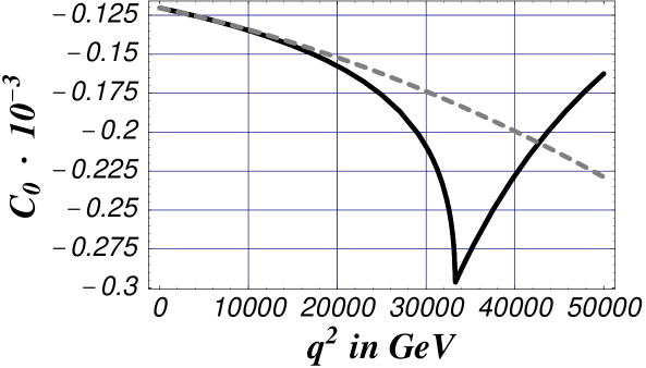
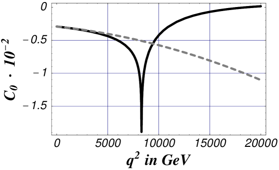
Finally, we compare our exactly analytical solutions with the numerical evaluation of the scalar three point functions $C_{0}$ using the computer program package LoopTools [30], as well as the aproximate analytical expressions found with the Taylor power series near $q^{2}=0$, used in some phenomenological applications in neutrino physics [31], [32].

In this regard, we have analyzed the Passarino-Veltman scalar three-point functions $C_{0}(q^{2},0,0;0,M_{{\scriptscriptstyle Z}}^{2},M_{{\scriptscriptstyle Z}}^{2})$ and $C_{0}(q^{2},0,0;m_{{\scriptscriptstyle e}}^{2},M_{{\scriptscriptstyle Z}}^{2},0)$ respectively, where $q^{2}$ denotes the photon momentum, $m_{{\scriptscriptstyle e}}$ and $M_{{\scriptscriptstyle Z}}$ are the electron and the vectorial boson $Z$ masses. The corresponding plots can be seen in Figures 2 and 3. The solid (black) line, in both graphics, shows the exact solution of Equations (12) and (14), perfectly matching the numerical evaluation using the aforementioned LoopTools package. The dashed (grey) line represents the aproximate solution of the Taylor expansion around $q^{2}=0$ whose expressions, up to ${\cal O}(q^{6})$ order, are

$$C_{0}(q^{2},0,0;0,M_{{\scriptscriptstyle Z}}^{2},M_{{\scriptscriptstyle Z}}^{2})\simeq-\frac{1}{M_{{\scriptscriptstyle Z}}^{2}}-\frac{q^{2}}{12\,M_{{\scriptscriptstyle Z}}^{4}}-\frac{q^{4}}{90\,M_{{\scriptscriptstyle Z}}^{6}}+{\cal O}(q^{6})$$

$$\begin{array}[]{c}\displaystyle C_{0}(q^{2},0,0;m_{{\scriptscriptstyle e}}^{2},M_{{\scriptscriptstyle Z}}^{2},0)\simeq\frac{\ln\Big{(}\frac{m_{{\scriptscriptstyle e}}^{2}}{M_{{\scriptscriptstyle Z}}^{2}}\Big{)}}{M_{{\scriptscriptstyle Z}}^{2}-m_{{\scriptscriptstyle e}}^{2}}+\frac{q^{2}}{2\,(m_{{\scriptscriptstyle e}}^{2}-M_{{\scriptscriptstyle Z}}^{2})^{3}}\Big{\{}(m_{{\scriptscriptstyle e}}^{2}-M_{{\scriptscriptstyle Z}}^{2})\Big{[}2-\ln\Big{(}\frac{m_{{\scriptscriptstyle e}}^{2}}{M_{{\scriptscriptstyle Z}}^{2}}\Big{)}\Big{]}\Big{\}}\\[14.22636pt] \displaystyle+\frac{q^{4}}{3\,(m_{{\scriptscriptstyle e}}^{2}-M_{{\scriptscriptstyle Z}}^{2})^{5}}\Big{\{}3\,(m_{{\scriptscriptstyle e}}^{4}-M_{{\scriptscriptstyle Z}}^{4})-(m_{{\scriptscriptstyle e}}^{4}+4\,m_{{\scriptscriptstyle e}}^{2}\,M_{{\scriptscriptstyle Z}}^{2}+M_{{\scriptscriptstyle Z}}^{4})\,\ln\Big{(}\frac{m_{{\scriptscriptstyle e}}^{2}}{M_{{\scriptscriptstyle Z}}^{2}}\Big{)}\Big{\}}+{\cal O}(q^{6})\end{array}$$

Note that our analytical solutions are valid for all $q^{2}$, in contrast to the aproximate solution, only valid when $q^{2}\rightarrow 0$, which physically means $q^{2}<<M_{Z}^{2}$

4 Summary and last remarks

In this paper, we have shown that the familiar scalar three-point function $C_{0}$ arising in Feynman diagram calculations, can be expressed in terms of eight Appell functions whose arguments are simple combinations of internal and external masses [23]. The extension to complex values of the masses (of concern in several interesting physical cases) can be performed via analytic continuation of the hypergeometric functions. Moreover, by invoking a theorem proved in [20] connecting dilogarithms and generalized hypergeometric functions, we have recovered a well-known formula for the evaluation of $C_{0}$ [18], [19]. Finally, let us stress that this work is on the line of searching for closed expressions of Feynman loop integrals. On the other hand but in a complementary way, such physical requirements should motivate, on the mathematical side, further developments of the still largely unknown field on multiple hypergeometric functions (as compared to one-variable hypergeometric functions) and their connections to generalized polylogarithms [15], [28].

Acknowledgments

M.A.S.L. has been partially supported by CICYT (Spain) under grant AEN-99/0692 and L.G.C.R. has been supported in part by the grants: Programa de Apoyo a Proyectos de Investigación e Innovación Tecnológica (PAPIIT) of the DGAPA-UNAM No. of Project: IN109001 (México) and in part by the Proyecto de Instalación of the CoNaCyT No. of Project: I37307-E (México).

References

• [1] P. Appell and J. Kampé de Fériet, Fonctions Hypergéometriques et Hyperesphériques. Polynomes d’Hermite, Gautiers-Villars, Paris (1926).
• [2] S. Bauberger, F.A. Berends, M. Böhm, M. Buza, Analytical and numerical methods for massive two-loop self-energy diagrams, Nucl. Phys. B 434 (1995) 383-407.
• [3] F.A. Berends, M. Böhm, M. Buza, R. Scharf, Closed expressions for specific massive multiloop self-energy diagrams, Z. Phys. C 63 (1994) 227-234.
• [4] L. Brücher, J. Franzkowski, D. Kreimer, A Program package calculating one-loop integrals, Comput. Phys. Commun. 107 (1997) 281-292.
• [5] A.I. Davydychev, Some exact results for N-point massive Feynman integrals, J. Math. Phys. 32 (1991) 1052-1058.
• [6] A.I. Davydychev, General results for massive N-point Feynman diagrams with different masses, J. Math. Phys. 33 (1992) 258-369.
• [7] A.I. Davydychev, Recursive algorithm for evaluating vertex-type Feynman integrals, J. Phys. A 25 (1992) 5587-5596.
• [8] A.I. Davydychev, Standard and hypergeometric representations for loop diagrams and the photon-photon scattering, hep-ph/9307323.
• [9] A.I. Davydychev and M.Yu. Kalmykov, New results for the $\epsilon$-expansion of certain one-, two- and three-loop Feynman diagrams, Nucl. Phys. B605 266-318 (2001), hep-th/0012189.
• [10] A.I. Davydychev and M.Yu. Kalmykov. Some remarks on the $\epsilon$-expansion of dimensionally regulated Feynman diagrams.Talk given at Zeuthen Workshop on Elementary Particle Theory: Loops and Legs in Quantum Field Theory, Koenigstein-Weissig, Germany, 9-14 Apr 2000. Nucl. Phys. Proc. Suppl. 89, 283-288 (2000), hep-th/0005287.
• [11] A. T. Suzuki and A. G. M. Schmidt, J. Phys. A31, 8023 - 8039 (1998).
• [12] C. Anastasiou, E.W.N. Glover and C. Oleari, Scalar one-loop integrals using the negative-dimension aproach, Nucl. Phys. B572, 307-360 (2000), hep-ph/9907494
• [13] H. Exton, Handbook of Hypergeometric Integrals, Ellis-Horwood, Chicester UK, 1978.
• [14] T. Hahn and M. Pérez-Victoria, Automatized one-loop calculations in four and D dimensions, UG-FT-87/98, hep-ph/9807565.
• [15] K.S. Kölbig, Nielsen’s generalized polylogarithms, SIAM J. Math. Anal. A7 (1987) 1232-1258.
• [16] L. Lewin, Polylogarithms and Associated Functions, North-Holland, New York 1981.
• [17] R. Mertig, R. Scharf, TARCER - A Mathematica program for the reduction of two-loop propagator integrals, hep-ph/9801383.
• [18] G.J. van Oldenborgh and J.A.M. Vermaseren, New algorithms for one-loop integrals, Z. Phys. C 46 (1990) 425-437.
• [19] G. Passarino and M. Veltman, One-Loop corrections for $e^{+}e^{-}$ annihilation into $\mu^{+}\mu^{-}$ in the Weinberg model, Nucl. Phys. B 160 (1979) 151-161.
• [20] M.A. Sanchis-Lozano, Simple connections between generalized hypergeometric series and dilogarithms, J. Comput. Appl. Math. 85 (1997) 325-331.Also available e-print archive:hep-ph/9511322.
• [21] M.A. Sanchis-Lozano, A Calculation of Scalar one-loop Integrals by means of generalized hypergeometric functions, IFIC/91-49.
• [22] M.A. Sanchis-Lozano, in preparation.
• [23] Luis G. Cabral-Rosetti and Miguel A. Sanchis-Lozano, J. Comp. Appl. Math. 115 (2000) 93-99. Also available e-print archive:hep-ph/9809213.
• [24] L.C. Joan Slater, Generalized Hypergeometric Functions, Cambridge University Press (1966).
• [25] H.M. Srivastava, M.C. Daoust, Nederl. Akad. Wetensch. Proc. A 72 (1969) 449-459.
• [26] O.V. Tarasov, A new approach to the momentum expansion of multiloop Feynman diagrams, Nucl. Phys. B 480 (1996) 397-412.
• [27] O.V. Tarasov, Generalized recurrence relations for two-loop propagator integrals with arbitrary mases, Nucl. Phys. B 502 (1997) 455.
• [28] O.V. Tarasov, Application and explicit solution of recurrence relations with respect to sapce-time dimension, Nucl. Phys. Proc. Suppl. 89, 237-245 (2000). Prepared for Zeuthen Workshop on Elementary Particle Theory: Loops and Legs in Quantum Field Theory, Koenigstein-Weissig, Germany, 9-14 Apr 2000. Also in *Bastei 2000, Loops and legs in quantum field theory* 237-245.
• [29] G. ’t Hooft and M. Veltman, Scalar one-loop integrals, Nucl.Phys. B 153 (1979) 365-401.
• [30] LoopTools is a package for evaluation of scalar and tensor one-loop integrals based on the FF package by G. J. van Oldenborgh. It features an easy Fortran, C++, and Mathematica interface to the scalar one-loop functions of FF and in addition provides the 2-, 3-, and 4-point tensor coefficient functions. LoopTools has been published in Comp. Phys. Comm. 118, 153 (1999), aviable e-print archive: hep-ph/9807565. FF has been published in Z. Phys. C46 425 (1990), aviable scanned version from KEK. We use the LoopTools User’s Guie, March 2000 by Thomas Hahn and LoopTools is aviable in:http://www.feynarts.de/looptools/
• [31] L. G. Cabral-Rosetti, J. Bernabèu, J. Vidal and A. Zepeda, Eur. Phys. J. C. 12, 633 (2000).
• [32] L. G. Cabral-Rosetti, Ph. D. Thesis “Factores de Forma del Neutrino e Invariancia Gauge Electrodébil: El Radio de Carga”, Departament de Física Teòrica, Facultad de Fisiques, Universitat de Valencia, Estudi General, 11 de Diciembre de 2000, Valencia, España.