${\tau-\mu}$  Flavor Violation as a Probe of the Scale of New Physics

Abstract

Motivated by the recent strong experimental evidence of large $\nu_{\mu}-\nu_{\tau}$ neutrino mixing, we explore current bounds on the analogous mixing in the charged lepton sector. We present a general formalism for dimension-6 fermionic effective operators involving $\tau-\mu$ mixing with typical Lorentz structure $(\overline{\mu}\,\Gamma\tau)(\overline{q}^{\alpha}\Gamma{q}^{\beta})$, and discuss their relationship to the standard model gauge symmetry and the underlying flavor dynamics. We derive the low-energy constraints on the new physics scale associated with each operator, mostly from current experimental bounds on rare decay processes of $\tau$, hadrons or heavy quarks. For operators involving at least one light quark ($u,d,s$), these constraints typically give a bound on the new physics scale of a few TeV or higher. Those operators with two heavy quarks turn out to be more weakly constrained at the present, giving bounds of a few hundred GeV. A few scalar and pseudo-scalar operators are free from all current experimental constraints.

I Introduction

The mystery of “flavor” poses a major challenge in particle physics. The unpredicted masses and mixings of three families of leptons and quarks in the flavor sector compose thirteen out of nineteen free parameters in the whole Standard Model (SM). Weak scale supersymmetry (SUSY) susy as a leading candidate for new physics beyond the SM provides no further understanding about the origin of flavor. In fact, it extends the mystery of flavor by necessarily adding three families of squarks and sleptons. Without additional assumptions for flavor structure of the soft SUSY breaking, supersymmetric theories often encounter phenomenolgical difficulties, known as the SUSY flavor problem susyf . In dynamical models of electroweak symmetry breaking, the phenomenological constraints on flavor-changing-neutral-currents (FCNC) make it hard for model building to accommodate the observed heavy top quark mass, unless new dynamics associated with the top quark is introduced Hill-Rept . Predicting the full mass spectrum and mixing pattern in the flavor sector may have to invoke new physics scales ranging from the weak scale up to very high scales in a single unified theory. Less ambitious and more practical approaches follow a “bottom-up” path, which effectively parametrize the new physics with flavor in a way not explicitly invoking unknown dynamics at the high scales. For instance, certain ansatze for fermion masses matrices were advocated ansatz , and realizations of horizontal symmetries were proposed FN ; NS to explain the fermion mass hierarchies and Cabibbo-Kobayashi-Maskawa (CKM) mixings CKM at relatively low scales. The FCNC fermionic Yukawa couplings to the Higgs sector can also be constructed in a phenomenologically viable way ansatzhiggs ; hall . When the electroweak symmetry breaking sector is nonlinearly realized CCWZ ; weinberg ; App , new FCNC gauge interactions of fermions can be economically described by effective operators of dimension-4 PZ ; BU ; while for the linearly realized Higgs sector, these couplings arise from dimension-6 effective operators BW .

The recent exciting evidence for neutrino oscillations atm ; sol strongly points to nonzero neutrino masses with large (rather than small) mixings which further discriminate the lepton sector from the quark sector and deepens the mystery of “flavor”. In fact, the atmospheric oscillation data atm favors maximal mixing between the $\mu$ and $\tau$ neutrinos via the Maki-Nakagawa-Sakata (MNS) matrix MNS . This development has led to a great amount of theoretical effort, with the hope of revealing the underlying new physics in the leptonic flavor sector numodel .

In this paper, we systematically explore the low energy constraints on effective operators induced by large $\tau-\mu$ mixing. This is strongly motivated by the neutrino oscillation data, in particular, the favored maximal mixing between the second and third generations via MNS matrix. Note that the large or maximal mixings in the MNS matrix may come from either neutrino mass diagonalization, or lepton mass diagonalization, or from both of them. It is indeed tempting to search for charged lepton flavor violations, in addition to the existing neutrino oscillation experiments. There are two classes of structures that can lead to flavor mixing for charged leptons. The first class is that there is no tree-level flavor mixing for charged leptons after mass diagonalization. This is an analogue to the SM quark sector, where the flavor mixing effects appear at tree level only in the charged current sector via the CKM mixing matrix. For instance, in a SM-like framework with additional mass and mixing parameters in the neutrino sector, $\tau-\mu$ mixing is generated at one-loop level and is generally suppressed by a factor of $m_{\nu}^{2}/M_{W}^{2}$, which would be negligible. The second class yields tree-level mixing effects after the mass diagonalization from the flavor eigenbasis into the mass eigenbasis. Typical theories in this class include extended models with extra $Z^{\prime}$ or Higgs doublets, generic weak-scale SUSY models, and dynamical models with compositeness, which often have rich structures of flavor mixing, leading to testable new phenomena. By contemplating on the large lepton mass hierarchy, dimensional analysis suggests the new physics scale associated with the mass and mixing of the third family leptons to be the lowest one in the lepton sector.

Before experiments can directly access the new physics scale associated with the lepton flavor sector, we use an effective theory formulation, obtained by integrating out the heavy degrees of freedom from a more fundamental theory. In Sec. II, we present our general formalism for the dimension-6 fermionic effective operators involving $\tau-\mu$ flavor mixing with typical Lorentz structures

$$\left(\bar{\mu}\,\Gamma\,\tau\right)(\bar{q}^{\alpha}\,\Gamma\,{q}^{\beta})\,,$$ (I.1)

where $\Gamma$ contains possible Dirac $\gamma$-matrices. This is beyond the simplest flavor-diagonal form of the effective four-Fermi contact interactions Peskin . With the operators in Eq. (I.1), we analyze their relationship to the realizations of the SM gauge symmetry and the underlying flavor dynamics. We further estimate the expected size of their coefficients, for a given cutoff scale at which the effective theory breaks down and new physics sets in. We also comment on to what extent our formalism can be applicable to loop-induced processes. In Sec. III, we systematically explore the constraints on the new physics scale associated with each operator, mostly from current experimental bounds on rare decays of $\tau$, hadrons or heavy quarks. For the operators involving at least one light quark ($u,d,s$), the current low energy constraints typically push the new physics scale to a few TeV or higher. Those operators with two heavy quarks are at the present subject to weaker constraints, only about a few hundred GeV. Some of the scalar and pseudo-scalar operators are free from any experimental constraint so far. We summarize our results in Table I and conclude in Sec. IV. Appendix A analyzes the relationship between our operators introduced in Sec. II and those with explicit SM gauge symmetry in both linear and non-linear realizations. In Appendix B, we further extend the above Eq. (I.1) to include the forms with generic lepton bilinear $\bar{{\ell}}^{\alpha}\,\Gamma\,{{\ell}}^{\beta}$, and derive the corresponding constraints from rare $\tau$ decays.

II Formalism for Effective Operators with $\tau\!-\!\mu$ Flavor Violation

II.1 Constructing the Dimension-6  $\tau\!-\!\mu$  Operators

We consider an effective theory below the new physics scale $\Lambda$, which can be generally defined as

$$\mathcal{L}_{\rm eff}=\mathcal{L}_{\rm SM}+\Delta\mathcal{L}$$ (II.2)

where $\mathcal{L}_{\rm SM}$ is the SM Lagrangian density and $\Delta\mathcal{L}$ denotes the new physics contribution via effective operators. For the current study, we will focus on the dimension-6 operators involving third and second family leptons $(\tau,\,\mu)$,

$$\Delta{\mathcal{L}}=\Delta{\mathcal{L}}^{(6)}_{\tau\mu}=\displaystyle\sum_{j,\alpha,\beta}\frac{~{}\mathcal{C}^{j}_{\alpha\beta}~{}}{\Lambda^{2}}\left(\overline{\mu}~{}\Gamma_{j}\,\tau\right)\left(\overline{q}^{\alpha}\,\Gamma_{j}\,q^{\beta}\right)\,+\,{\rm H.c.}\,,$$ (II.3)

where $\Gamma_{j}\in\left(1,\,\gamma_{5}^{~{}},\,\gamma_{\sigma}^{~{}},\,\gamma_{\sigma}^{~{}}\gamma_{5}^{~{}}\right)$ denotes relevant Dirac matrices, specifying scalar, pseudoscalar, vector and axial vector couplings, respectively. We will not consider the possibility that $\Gamma$ has tensor structure due to the following reasons: (a) there are no two-body decays involving the tau with tensor structure, and thus any bound would be extremely weak; (b) the tensor matrix elements involving quark bilinears are either unknown or known very poorly, and thus bounds would be not only very weak, but also rather uncertain; (c) the tensor structure does not generically appear in most models that we know. Here, we consider $\Gamma_{j}$ to be the same for both $\tau-\mu$ and $q^{\alpha}-q^{\beta}$ bilinears, where $\alpha$ and $\beta$ run over all allowed combinations of quark flavors. Under these considerations, we can show that Eq. (II.3) is the most general form (containing one $\tau-\mu$ bilinear and one quark-bilinear) which respects the unbroken $U(1)_{\rm em}$ gauge symmetry. As shown in the Appendix A, the operator Eq. (II.3) corresponds to a nonlinear realization of the electroweak gauge symmetry under which all fields feel only the unbroken $U(1)_{\rm em}$. For the linearly realized electroweak gauge symmetry where the physical Higgs and would-be Goldstone bosons form the usual Higgs doublet, the dimension-6 $\tau-\mu$ operators have to respect the full electroweak gauge group ${\cal G}_{\rm SM}=SU(2)_{L}\otimes U(1)_{Y}$ and are thus found to have a more restricted form,

$$\Delta{\mathcal{L}}^{\rm linear}=\Delta{\mathcal{L}}^{{\rm linear}}_{\tau\mu(6)}=\displaystyle\sum_{\alpha,\beta,\chi,\zeta}^{j}\frac{~{}\mathcal{C}^{j\chi\zeta}_{\alpha\beta}~{}}{\Lambda^{2}}\left(\overline{\mu_{\chi}}~{}\Gamma_{j}\,\tau_{\chi}\right)\left(\overline{q}_{\zeta}^{\alpha}\,\Gamma_{j}\,q_{\zeta}^{\beta}\right)\,+\,{\rm H.c.}\,,$$ (II.4)

where the chirality indices $\chi,\zeta=L,R$. This restricts $\Gamma\in(\gamma^{~{}}_{\sigma},\,\gamma_{\sigma}^{~{}}\gamma^{~{}}_{5})$, so that Eq. (II.4) only belongs to a sub-set of operators in Eq. (II.3).  At first sight, this is somewhat surprising as the scalar and pseudoscalar operators in Eq. (II.3) are fully absent at dimension-6. However, it is interesting to note that such scalar and pseudoscalar structures reappear in the dimension-8 effective operators,

$$\begin{array}[]{ll}\Delta{\mathcal{L}}^{{\rm linear}}_{\tau\mu(8)}\!\!\!&=\displaystyle\frac{1}{\Lambda^{4}}\!\!\!\displaystyle\sum_{\alpha,\beta,\alpha^{\prime},\beta^{\prime}}^{j}\!\!\!\mathcal{C}^{j(8)}_{\alpha\beta\alpha^{\prime}\beta^{\prime}}\!\left(\overline{L}_{\ell}^{\alpha^{\prime}}\Phi\Gamma_{j}\,\ell_{R}^{\beta^{\prime}}\right)\!\!\left(\overline{L}_{q}^{\alpha}\Phi^{\prime}\Gamma_{j}\,q_{R}^{\beta}\right)\!+\!\widetilde{\mathcal{C}}^{j(8)}_{\alpha\beta\alpha^{\prime}\beta^{\prime}}\!\left(\overline{L}_{\ell}^{\alpha^{\prime}}\Phi\Gamma_{j}\,\ell_{R}^{\beta^{\prime}}\right)\!\!\left(\overline{q_{R}}^{\beta}\Phi^{\prime{\dagger}}\Gamma_{j}\,L_{q}^{\alpha}\right)\!+\!{\rm H.c.}\\[17.07164pt] &\Rightarrow\displaystyle\sum_{\alpha,\beta}^{j}\frac{v^{2}\widehat{\mathcal{C}}^{j(8)}_{\alpha\beta}}{2\Lambda^{4}}\left(\overline{\mu}~{}\Gamma_{j}\,\tau\right)\left(\overline{q}^{\alpha}\,\Gamma_{j}\,q^{\beta}\right)\,+\,{\rm H.c.}\,,~{}~{}~{}~{}~{}\left(\,{\rm for}~{}\Phi=\langle\Phi\rangle\,\right),\end{array}$$ (II.5)

where $\Gamma_{j}\in(1,\,\gamma_{5})$, $L_{\ell}\,(L_{q})$ is the left-handed lepton (quark) doublet, and $\Phi$ is the Higgs doublet with hypercharge $\frac{1}{2}$ and vacuum expectation value (VEV) $\langle\Phi\rangle=v/\sqrt{2}\left(0,\,1\right)^{T}$. We also denote, in Eq. (II.5), $\Phi^{\prime}=\Phi$ for $q_{R}=d_{R}^{~{}}$ and $\Phi^{\prime}=i\tau_{2}\Phi^{\ast}$ for $q_{R}=u_{R}^{~{}}$. Note that when the Higgs doublet takes its VEV, the dimension-8 operators in Eq. (II.5) reduce to the generic dimension-6 form in Eq. (II.4) but with coefficients further suppressed by an extra factor of $v^{2}/(2\Lambda^{2})$. Thus, they can be neglected in comparison with the leading dimension-6 operators Eq. (II.4). This means that for the linear realization of the SM gauge symmetry, only vector and axial-vector operators with $\Gamma_{j}\in(\gamma_{\sigma},\,\gamma_{\sigma}\gamma_{5})$ are relevant at dimension-6 level. For the phenomenological analysis in Sec. III, we will focus on analyzing the bounds for the most general form in Eq. (II.3) since Eq. (II.3) contains the restricted form in Eq. (II.4) as a special case.

Finally, we note that in principle, we could also include purely leptonic dimension-6 operators of the form $\left(\bar{\mu}\,\Gamma\,\tau\right)(\overline{{\ell}}^{a}\,\Gamma\,{\ell}^{\beta})$, which contains an additional lepton bilinear $(\overline{{\ell}}^{a}\,\Gamma\,{\ell}^{\beta})$ instead of quark bilinear $(\overline{q}^{a}\,\Gamma\,q^{\beta})$. They may involve similar flavor dynamics as the effective operators (II.3), but unlike (II.3) they are relevant to only a few low energy constraints. Most nontrivial bounds come from certain three-body rare $\tau$ decays and all appear similar. We will summarize these separately in Appendix B.

II.2 Theoretical Consideration for the Size of Coefficients

The precise value of the dimensionless coefficient $\mathcal{C}^{j}_{\alpha\beta}$ in Eq. (II.3) should be derived from the corresponding underlying theory in principle. In the current effective theory analysis, we will invoke a power counting estimate. As shown in the Appendix A, the operator Eq. (II.3) is formulated under the nonlinear realization of the SM gauge group ${\cal G}_{\rm SM}$, which provides a natural effective description of the strongly coupled electro-weak symmetry breaking (EWSB) sector and/or compositeness. In this scenario, the natural size of $\mathcal{C}^{j}_{\alpha\beta}$ for an effective dimension-6 four-Fermi operator such as (II.3) can be typically estimated as Hill-Rept ,

$$\mathcal{C}^{j}_{\alpha\beta}~{}=~{}4\pi\,\mathcal{O}(1)\,,~{}~{}~{}~{}~{}({\rm default}),$$ (II.6)

which corresponds to an underlying theory with a strong gauge coupling $\alpha_{S}^{~{}}=g_{S}^{2}/4\pi=\mathcal{O}(1)$. Naive dimensional analysis (NDA) georgi1 ; georgi2 provides another way to estimate operators in the nonlinear realization. For the dimension-6 operators in Eq. (II.3), the NDA gives

$$\mathcal{C}_{\alpha\beta}^{j}[{\rm NDA}]~{}\lesssim~{}(4\pi)^{2}\,\mathcal{O}(1)\,.$$ (II.7)

which corresponds to an underlying theory with a strong gauge coupling   $\alpha_{S}=g_{S}^{2}/4\pi\lesssim\mathcal{O}(4\pi)$ . So, in general, for the nonlinearly realized effective theory, we expect $\mathcal{C}^{j}_{\alpha\beta}\gtrsim 4\pi$,  and to be conservative we will choose the estimate Eq. (II.6) as the “default” value of our analysis. With Eq. (II.6), all the phenomenological bounds derived in the next section can be translated into bounds on the new physics scale $\Lambda$. The bounds with a different counting of $\mathcal{C}^{j}_{\alpha\beta}$, such as Eq. (II.7) above and Eq. (II.8) below, can be directly obtained from our default results by simple rescaling.

In the weakly coupled theories, we have

$$\mathcal{C}_{\alpha\beta}^{j}~{}=~{}\mathcal{O}(1)\,,~{}~{}~{}~{}~{}({\rm weakly~{}coupled~{}scenario}).$$ (II.8)

Since the new physics scale of a weakly coupled scenario is likely to be first determined by discovering the light new particles (such as light Higgs boson(s) and a few lower-lying states of superpartners), we may mainly motivate the current analysis by the strongly coupled theories where the estimate in Eq. (II.6) or (II.7) can sensibly apply. However, as will be clear from the Sec. III and IV below, even for the weakly coupled theories with Eq. (II.8), significant bounds on the new physics scale $\Lambda$ can still be derived for the operators with the quark-bilinear $\bar{q}^{\alpha}\,\Gamma\,q^{\beta}$ containing no $t$ quarks, no $c$ quarks and at most one $b$ quark.

The linear realization is more appropriate when there is a Higgs boson with a mass well below the scale $4\pi v\simeq 3.1$ TeV, such as in the typical models with supersymmetry susy or composite Higgs models with Top-color Hill-Rept . Finally, we note that the above estimates for the coefficient are flavor-blind, i.e., we do not worry about the possible suppression from flavor-violation effects. Below we will analyze how the large leptonic $\tau-\mu$ flavor mixing is naturally realized in typical scenarios without further suppression.

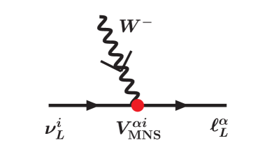
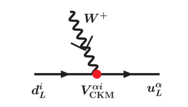
Figure 1: The charged current interactions for lepton sector involving MNS mixings (left plot), and for quark sector involving CKM mixings (right plot).

II.3 Neutrino Oscillations, Large Lepton Mixings and  $\tau\!-\!\mu$  Flavor Violation Operators

Neutrino oscillation experiments can measure the lepton charged current interactions involving (large) MNS mixings (cf. left plot in Fig. 1) analogous to the quark charged current interactions involving (small) CKM mixings (cf. right plot in Fig. 1). Thus we can generally write,

$${\mathcal{L}}^{\ell}_{CC}=\displaystyle-\frac{g}{\sqrt{2}}\sum^{\alpha=e,\mu,\tau}_{i=1,\cdots,N}\overline{\ell_{L}}^{\alpha}\gamma^{\rho}\,V_{\alpha i}\,\nu_{L}^{i}W^{-}_{\rho}\,+\,{\rm H.c.}$$ (II.9)

where $V$ is the $3\times N$ unitary MNS mixing matrix containing a product of two left-handed rotation matrices,

$$V_{\alpha i}=\displaystyle\sum_{\beta=1}^{3}U^{\ell\,\ast}_{L\,\beta\alpha}U^{\nu}_{L\,\beta i}~{},$$ (II.10)

where $U^{\ell}_{L}$ ($3\times 3$) is from the lepton mass diagonalization  $U^{\ell\,{\dagger}}_{L}M_{\ell}U^{\ell}_{R}=M_{\ell}^{\rm diag}$  and  $U^{\nu}_{L}$  ($N\times N$) is from diagonalizing the neutrino mass matrix (of Majorana or Dirac type). Hence, the large or maximal mixings in the MNS matrix $V$ can originate from (i) either $U^{\nu}_{L}$ (neutrino mass diagonalization), (ii) or $U^{\ell}_{L}$ (left-handed lepton mass diagonalization), (iii) or both sources. In the cases (ii) and (iii), we see that large mixings in $U^{\ell}_{L}$ play important roles for neutrino oscillation phenomena. Furthermore, the right-handed lepton rotation $U^{\ell}_{R}$ does not enter the MNS matrix and is thus free from the constraint of oscillation experiments. This means that even in the case (i) large lepton mixings can originate from $U^{\ell}_{R}$ though $U^{\ell}_{L}$ is constrained to have only small mixings. Clearly, the neutrino oscillation data alone could not identify the origin of the MNS mixings (involving only the product of two left-handed rotations), i.e., whether the large or maximal mixings in MNS matrix really originate from the neutrino mass matrix or charged lepton mass matrix or both .  Therefore, to fully understand the flavor dynamics in the lepton and neutrino sector, it is important to directly test lepton rotation matrices $U^{\ell}_{L}$ and $U^{\ell}_{R}$ in other lepton flavor-violation processes. The large or maximal MNS mixings observed in the neutrino oscillation experiments strongly motivate searches for large lepton flavor-violating interactions originating from $U^{\ell}_{L}$ and $U^{\ell}_{R}$ .

The effective dimension-six $\tau-\mu$ operator Eq. (II.3) can arise from exchange of certain heavy particles such as a heavier neutral gauge boson ($Z^{\prime}$), or a heavier Higgs scalar ($S^{0}$). The underlying dynamics for such interactions fall into two distinct classes: (a). flavor universal, or, (b). flavor non-universal. For the Class-(a), we can write a generic lepton-bilinear term $\overline{\psi}\,\Gamma_{j}\,\psi$, where $\psi=\left(e,\,\mu,\,\tau\right)^{T}$. We thus deduce

$$\overline{\psi}\,\Gamma_{j}\,\psi=\left\{\begin{array}[]{l}\displaystyle\sum_{\chi(\neq\zeta)}\overline{\psi_{\chi}}\,\Gamma_{j}\,\psi_{\zeta}\,,~{}~{}~{}~{}~{}(\Gamma_{j}=1,\,\gamma_{5});\\[17.07164pt] \displaystyle\sum_{\chi}\overline{\psi_{\chi}}\,\Gamma_{j}\,\psi_{\chi}\,,~{}~{}~{}~{}~{}(\Gamma_{j}=\gamma_{\sigma},\,\gamma_{\sigma}\gamma_{5});\end{array}\right.$$ (II.11)

where $\chi,\zeta=L,R$. The lepton mass diagonalization $U^{\ell\,{\dagger}}_{L}M_{\ell}U^{\ell}_{R}=M_{\ell}^{\rm diag}$ enables us to transform leptons from flavor-eigenbasis ($\psi$) into mass-eigenbasis ($\psi^{\prime}$) via $\psi_{L}=U^{\ell}_{L}\psi_{L}^{\prime}$ and $\psi_{R}=U^{\ell}_{R}\psi_{R}^{\prime}$. Thus, Eq. (II.11) can be rewritten as, in the mass-eigenbasis,

$$\overline{\psi}\,\Gamma_{j}\,\psi=\left\{\begin{array}[]{l}\displaystyle\sum_{\chi(\neq\zeta)}\overline{\psi_{\chi}^{\prime}}\,\Gamma_{j}\left(U_{\chi}^{\ell\,{\dagger}}U_{\zeta}^{\ell}\right)\psi_{\zeta}^{\prime}~{}\Rightarrow~{}\mathcal{O}(1)\,\overline{\tau^{\prime}}\Gamma_{j}\,\mu^{\prime}+\mathcal{O}(1)\,\overline{\mu^{\prime}}\Gamma_{j}\tau^{\prime},~{}~{}~{}~{}(\Gamma_{j}=1,\,\gamma_{5})\,;\\[17.07164pt] \displaystyle\sum_{\chi}\overline{\psi_{\chi}^{\prime}}\,\Gamma_{j}\,\psi_{\chi}^{\prime}\,,~{}~{}~{}~{}(\Gamma_{j}=\gamma_{\sigma},\,\gamma_{\sigma}\gamma_{5})\,.\end{array}\right.$$ (II.12)

Here, for $\Gamma_{j}=1,\,\gamma_{5}$, the unsuppressed $\tau^{\prime}-\mu^{\prime}$ mixing bilinears can be induced by the large $\mathcal{O}(1)$ “23” or “32” entries in the lepton rotation matrices $U_{L}^{\ell\,{\dagger}}U_{R}^{\ell}$ and $U_{R}^{\ell\,{\dagger}}U_{L}^{\ell}$.  We see that such large flavor-mixings between $\tau^{\prime}$ and $\mu^{\prime}$ occur only for $\Gamma=1,\,\gamma_{5}$, implying that for Class-(a) the $\tau-\mu$ operators arise from exchanging a heavy scalar (pseudoscalar) in the underlying theory (cf. Fig. 2b and 2c). For scalar (pseudoscalar) type couplings to be flavor universal, there should be certain flavor symmetry associated with these couplings in the underlying theory. The quark bilinear $\overline{Q}\Gamma_{j}Q$ can join the same type of flavor universal interactions, where $Q={\cal U},\,{\cal D}$ with ${\cal U}=(u,\,c,\,t)^{T}$ and ${\cal D}=(d,\,s,\,b)^{T}$. But, without fine-tuning the flavor-violations in the quark-bilinear would be relatively small based on the experimental knowledge about the CKM matrix, except that some right-handed mixings may be quite sizable.

We then proceed to consider Class-(b) with flavor non-universal dynamics which is strongly motivated by the observed large mass hierarchies for leptons and quarks. For instance, the induced lepton-bilinear may contain only the third family tau-leptons as happened in the dynamical symmetry breaking models Hill-Rept ; Hill-tc ; Chiv and lepton non-universality models Ma ; EL ; Zhang . Generically, we can write down a tau-lepton bilinear in the flavor eigenbasis,  $\overline{\tau_{\chi}}\,\Gamma_{j}\,\tau_{\zeta}$  where $\chi=\zeta$ corresponds to gauge boson $Z^{\prime}$ exchange and $\chi\neq\zeta$ corresponds to scalar $S^{0}$ exchange. The $Z^{\prime}$ exchange from the strongly interacting theories such as top-color models Hill-tc is particularly interesting for studying the effective dimension-6 operators (II.3) as the $Z^{\prime}$ induces strong couplings for Eq. (II.3) which naturally fit the counting in Eq. (II.6). Because of the flavor non-unversality of such underlying dynamics, the generic tau-lepton bilinear takes the following form after the lepton mass-diagonalization,

$$\overline{\tau_{\chi}}\,\Gamma_{j}\,\tau_{\zeta}=\overline{\ell_{\chi}^{\prime\alpha}}\,\Gamma_{j}\,(U_{\chi}^{\ell\,\ast})_{3\alpha}(U_{\zeta}^{\ell})_{3\beta}\,\ell_{\zeta}^{\prime\beta}~{}\Rightarrow~{}\mathcal{O}(1)\,\overline{\tau^{\prime}}\,\Gamma_{j}\,\mu^{\prime}+\mathcal{O}(1)\,\overline{\mu^{\prime}}\,\Gamma_{j}\,\tau^{\prime}\,,$$ (II.13)

where $\chi\neq\zeta$ for $\Gamma_{j}=1,\,\gamma^{~{}}_{5}$ and $\chi=\zeta$ for $\Gamma_{j}=\gamma^{~{}}_{\sigma},\,\gamma^{~{}}_{\sigma}\gamma^{~{}}_{5}$. We see that, due to the allowed large entry $(U_{L}^{\ell})_{32}$ or $(U_{R}^{\ell})_{32}$, the un-suppressed flavor-violating $\tau-\mu$ bilinear can be generated for $\Gamma_{j}$ being either (axial-)vector or (pseudo-)scalar (cf. Fig. 2a-c), unlike the situation in Eq. (II.12). In most cases, such flavor non-universal dynamics generically invokes the third family quark-bilinears $\overline{t_{\chi}}\,\Gamma_{j}\,t_{\zeta}$ and $\overline{b_{\chi}}\,\Gamma_{j}\,b_{\zeta}$ at the same time, and some sizable right-handed mixings such as $t_{R}^{~{}}\!-\!c_{R}^{~{}}$ mixing (or $b_{R}^{~{}}\!-\!s_{R}^{~{}}$ mixing) can naturally arise HY . To be model-independent, we will include all possible flavor combinations in the quark-bilinear $\overline{q}^{\alpha}\,\Gamma_{j}\,q^{\beta}$ [cf. Eq. (II.3)] for our phenomenological analysis in the next section.

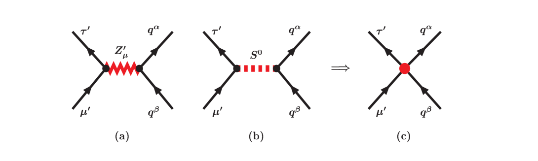
Figure 2: Illustration of typical generations of the effective four-Fermi interactions [cf. Eq. (II.3)] in plot (c) from the exchange of (a) a heavy new gauge boson $Z_{\mu}^{\prime}$, or, (b) a heavy new scalar or pseudoscalar $S^{0}$ in the underlying theories. Here the $\tau^{\prime}-\mu^{\prime}$ flavor-violation couplings solely come from the charged lepton mass-diagonalization matrices $U^{\ell}_{L}$ and/or $U^{\ell}_{R}$.

In summary, a full understanding of leptonic flavor dynamics (for both masses and mixings) requires experimental exploration not only via neutrino oscillations but also via other lepton-flavor-violating processes. The above classification shows that, given the large lepton mixings (especially for the tau and muon leptons) as motivated by the atmospheric neutrino oscillation data, the effective dimension-six flavor-violating $\tau-\mu$ operators (II.3) can be naturally realized without additional suppression (in contrast to the quark sector). Furthermore, particular chirality structures (characterized by $\Gamma_{j}$) can be singled out, depending on whether the underlying leptonic dynamics is universal or non-universal in the flavor space. The systematic phenomenology constraints analyzed in the following Sec. III will demonstrate how the various low energy precision data on lepton flavor-violations can probe the new physics scale associated with the underlying flavor dynamics, complementary to the neutrino oscillation experiments.

II.4 Radiative Corrections versus Leading Logarithmic Term

In our analysis, we will consider two classes of bounds, from contributions at either the tree level or the loop level. Many of these bounds arise from the tree-level operators (II.3) directly and will be derived from various low energy decay channels. In some cases, the significant bounds can only be obtained by relating the operators involving one set of heavy quarks to those involving lighter quarks, through exchange of a $W$ or charged Goldstone boson at the loop level (cf., Fig. 3 in Section 3). How does one handle radiative loop effects in an effective theory? For such calculations, typically, some loop integrals are divergent and must be cut off at a scale $\Lambda$. In the case of $W$ or Goldstone boson exchange, the divergence is logarithmic. We perform the loop integral by retaining the leading logarithmic terms in which the ultraviolet (UV) cutoff $\Lambda$ would reliably represent the scale of new physics BL . In doing the analysis, we assume only one $(\bar{\mu}\Gamma_{j}\tau)(\bar{q}^{\alpha}\Gamma_{j}q^{\beta})$ operator to be non-zero. Other diagrams involving closed fermion loops may have quadratic divergences. Unlike the logarithmic terms, such $\mathcal{O}(\Lambda^{2})$ power corrections are not guaranteed to always represent the real contributions of the lowest heavy physical state of a mass $M_{\rm phys}$, so that to be conservative it is usually suggested BL that one only uses the logarithmic terms ($\sim\ln\Lambda$) computed in the effective theory, for representing the new physics contribution ($\sim\ln M_{\rm phys}$) from an underlying full theory. We will take this approach for the loop analysis in Section 3, though we keep in mind that retaining only leading logarithms may possibly underestimate the new physics loop-contributions if the $\mathcal{O}(M_{\rm phys}^{2})$ terms are not vanishing in a given underlying theory. This exception occurs only when the heavy mass effect in the underlying theory does not obey the usual decoupling theorem DCT . Thus, extracting the possible nonzero $\mathcal{O}(M_{\rm phys}^{2})$ terms is a highly model-dependent issue and is hard to generally handle in an effective theory formalism. The traditional “leading logarithm” approach provides a conservative estimate for the effective theory analysis and is justified for those underlying theories in which the effects of the heavy states (integrated out from the low energy spectrum) exhibit the decoupling behavior.

III Phenomenological Constraints

We consider the general $\tau-\mu$ operators in Eq. (II.3) and take $\Gamma_{j}$ to be the same for both the lepton and quark pieces. There are four types of operators to be considered, $\Gamma_{j}=(S,P,V,A)$, and for each type there are twelve combinations of $q_{\alpha}q_{\beta}$, $(uu,dd,ss,cc,bb,tt,ds,db,sb,uc,ut,ct)$. This gives a total of 48 operators for our analysis. We first consider operators involving two light quarks ($uu,dd,ss,ds$), then the non-diagonal operators involving one or more heavy quarks ($db,sb,uc,ut,ct$), and finally consider the diagonal operators involving two heavy quarks ($cc,bb,tt$). In our analysis, we will consider one operator to be nonzero at a time and derive the corresponding bound on the new physics scale $\Lambda$. This should provide a sensible estimate of the scale $\Lambda$ under the naturalness assumption mentioned in Section II, which states that there is no accidental cancellation among the contributions of different operators.

III.1 Operators with Two Light Quarks

For operators with two light quarks, the neutrinoless decay of the $\tau$ into a $\mu$ and one or more light mesons will provide the best bound. First, we establish our conventions: The PCAC condition for the pseudoscalar octet gives

$$\left<0\left|j_{\mu}^{(5)b}(0)\right|\phi^{a}(p)\right>=i\delta^{ab}\frac{F_{\phi}}{\sqrt{2}}p_{\mu}\,,$$ (III.14)

where $F_{\phi}$ is the meson decay constant and the Cartesian components of the axial vector current are

$${j^{\mu}}^{(5)b}=\bar{q}\gamma^{\mu}\gamma^{5}\frac{\lambda^{b}}{2}q\,.$$ (III.15)

Here $\phi=\phi^{a}\lambda^{a}/{\sqrt{2}}$ with $a=1\cdots 8$ is the $3\times 3$ matrix of pseudoscalar meson fields and $\lambda^{a}$ are the Gell-Mann matrices normalized according to ${\rm Tr}(\lambda^{a}\lambda^{b})=2\delta^{ab}$. For current quark masses, we choose

$$m_{u}=m_{d}=5\ {\rm MeV}\,,\quad{\rm and}\quad m_{s}=120\ {\rm MeV}\,,$$ (III.16)

and the results are not particularly sensitive to these choices. For simplicity, the muon mass (and the pion mass, when applicable) will be neglected relative to the tau mass when calculating kinematics.

Knowing the vacuum transition matrix element, we can readily evaluate the particle decay width. For instance, for a two-body decay $\tau\rightarrow\mu M$ where $M$ is a generic light meson, we have the spin-summed and averaged partial width

$$\Gamma(\tau\rightarrow\mu M)={1\over 2m_{\tau}}{1\over(8\pi)}\overline{\sum}|{\cal M}|^{2},$$ (III.17)

where the transition amplitude $i{\cal M}=<\mu M|i{\cal H}|\tau>$ can be evaluated by vacuum insertion.

$\bullet$ Axial Vector Operators

Bounds on the $uu$ and $dd$ axial operators can be obtained by looking at $\tau\rightarrow\mu\pi^{0}$. Using

$$\left<0\left|\bar{u}\gamma^{\mu}\gamma^{5}u\right|\pi^{0}(p)\right>=\left<0\left|\bar{q}\gamma^{\mu}\gamma^{5}\left(\frac{1}{2}+\frac{\lambda^{3}}{2}\right)q\right|\phi^{3}(p)\right>=i\frac{F_{\pi}}{\sqrt{2}}p_{\mu}$$ (III.18)

with $F_{\pi}=131\ {\rm MeV}$, and noting that for $u\rightarrow d$ the right-hand side is the same except with an opposite sign, we find

$$\Gamma\left(\tau\rightarrow\mu\pi^{0}\right)=\frac{1}{\Lambda^{4}}\frac{\pi}{2}F_{\pi}^{2}m_{\tau}^{2}<0.908\times 10^{-17}~{}{\rm GeV}\,,$$ (III.19)

where the inequality comes from the $90\%$ C.L. experimental bound on this decay mode listed in Ref. pdg . This then implies that, for both the  $\bar{u}\gamma^{\mu}\gamma^{5}u$  and  $\bar{d}\gamma^{\mu}\gamma^{5}d$  operators,

$$\Lambda>11.3~{}{\rm TeV}\,.$$ (III.20)

For the $ss$ axial operator, a bound is obtained from $\tau\rightarrow\mu\eta$. We have

$$\left<0\left|\bar{s}\gamma^{\mu}\gamma^{5}s\right|\eta(p)\right>=i\frac{-2}{\sqrt{3}}\frac{F_{\eta}}{\sqrt{2}}\,p^{\mu}\,,$$ (III.21)

where $\displaystyle F_{\eta}=F_{\eta}^{8}-\displaystyle\frac{1}{\sqrt{2}}F_{\eta}^{0}$ is defined using $\left<0\left|\bar{q}\gamma^{\mu}\gamma^{5}\frac{\lambda^{8,0}}{2}q\right|\eta(p)\right>=i\frac{F_{\eta}^{8,0}}{\sqrt{2}}p_{\mu}$. Here,  $\lambda^{0}=\displaystyle{\sqrt{\frac{2}{3}}}\,$1  and at the next-to-leading order (NLO) of the chiral perturbation theory feldman , $F_{\eta}^{8}=154\ {\rm MeV}$ and $F_{\eta}^{0}=25\ {\rm MeV}$. Using these values we find that $F_{\eta}\approx F_{\pi}$, the value from the ${\mathrm{S}U(3)}$ limit. This gives,

$$\Gamma(\tau\rightarrow\mu\eta)=\frac{2\pi}{3}\frac{{\left(m_{\tau}^{2}-m_{\eta}^{2}\right)}^{2}}{m_{\tau}}\frac{F_{\eta}^{2}}{\Lambda^{4}}<2.179\times 10^{-17}~{}{\rm GeV}\,,$$ (III.22)

implying

$$\Lambda>9.5~{}{\rm TeV}.$$ (III.23)

Note that, for the isospin-invariant effective operator $\displaystyle\frac{4\pi}{\Lambda^{2}}\left(\bar{\mu}A\tau\right)\left(\bar{u}Au+\bar{d}Ad\right)$ with $A=\gamma^{\mu}\gamma^{5}$, the same bound of $\Lambda>9.5$ TeV can be derived from the above process.

For the $sd$ operator, the bound comes from $\tau\rightarrow\mu K^{0}$. Thus, we have

$$\left<0\left|\bar{s}\gamma^{\mu}\gamma^{5}d\right|K^{0}\right>=iF_{K}p^{\mu}\,,$$ (III.24)

where experimentally $F_{K}=160\ {\rm MeV}$. This leads to

$$\Gamma(\tau\rightarrow\mu K^{0})=\pi\frac{{\left(m_{\tau}^{2}-m_{K}^{2}\right)}^{2}}{m_{\tau}}\frac{F_{K}^{2}}{\Lambda^{4}}<2.27\times 10^{-15}~{}{\rm GeV}\,,$$ (III.25)

and thus,

$$\Lambda>3.6~{}{\rm TeV}.$$ (III.26)

$\bullet$ Pseudoscalar Operators

Here, the Dirac equation is used to reduce the axial vector matrix elements to pseudoscalar matrix elements, and then we use the same processes as above.

We find that

$$\left<0\left|\bar{u}\gamma^{5}u\right|\pi^{0}(p)\right>=-\left<0\left|\bar{d}\gamma^{5}d\right|\pi^{0}(p)\right>=\frac{i}{\sqrt{2}}\frac{m_{\pi}^{2}}{~{}m_{u}+m_{d}~{}}F_{\pi}\,,$$ (III.27)

which then yields

$$\Gamma(\tau\rightarrow\mu\pi^{0})=\frac{\pi}{8}\frac{F_{\pi}^{2}m_{\pi}^{4}m_{\tau}}{\Lambda^{4}m_{q}^{2}}<0.908\times 10^{-17}~{}{\rm GeV}\,,$$ (III.28)

so that

$$\Lambda>11.7~{}{\rm TeV}.$$ (III.29)

For the strange quark operator, we find

$$\left<0\left|\bar{s}\gamma^{5}s\right|\eta_{8}(p)\right>=-i{\sqrt{6}}\,F_{\eta}^{8}\frac{m_{\eta_{8}}^{2}}{~{}m_{u}+m_{d}+4m_{s}~{}}$$ (III.30)

which gives (taking $\eta=\eta_{8}$)

$$\Gamma(\tau\rightarrow\mu\eta)=\frac{6\pi}{\Lambda^{4}}\frac{m_{\eta}^{4}{F_{\eta}^{8}}^{2}}{{\left(m_{u}+m_{d}+4m_{s}\right)}^{2}}\frac{{\left(m_{\tau}^{2}-m_{\eta}^{2}\right)}^{2}}{m_{\tau}^{3}}<2.18\times 10^{-17}~{}{\rm GeV}\,,$$ (III.31)

implying

$$\Lambda>9.9~{}{\rm TeV}.$$ (III.32)

For the isospin-invariant effective operator $\displaystyle\frac{4\pi}{\Lambda^{2}}\left(\bar{\mu}P\tau\right)\left(\bar{u}Pu+\bar{d}Pd\right)$ with $\,P=\gamma^{5}$,  the same bound of $\Lambda>9.9$ TeV can be derived from the above process.

Finally, we have

$$\left<0\left|\bar{s}\gamma^{5}d\right|K^{0}\right>=i\frac{m_{K^{0}}^{2}}{m_{d}+m_{s}}F_{K}\,,$$ (III.33)

which gives

$$\Gamma(\tau\rightarrow\mu K^{0})=\frac{\pi}{\Lambda^{4}}\frac{m_{K}^{4}{F_{K}}^{2}}{{\left(m_{d}+m_{s}\right)}^{2}}\frac{{\left(m_{\tau}^{2}-m_{K}^{2}\right)}^{2}}{m_{\tau}^{3}}<2.27\times 10^{-15}~{}{\rm GeV}\,.$$ (III.34)

Thus, we deduce

$$\Lambda>3.7~{}{\rm TeV}.$$ (III.35)

$\bullet$ Vector Operators

We take a simple ${\mathrm{S}U(3)}$ relation:

$$\left<0\left|\bar{q}\gamma^{\mu}\frac{\lambda^{a}}{2}q\right|V^{b}\right>=i\epsilon^{\mu}\delta^{ab}\frac{c}{\sqrt{2}}\,,$$ (III.36)

where $V_{\mu}=\displaystyle V_{\mu}^{a}\frac{\lambda^{a}}{\sqrt{2}}$ is the vector meson octet. Using vector meson dominance sakurai , we determine the dimensionless ratio $g\equiv m^{2}/c$ from $V\rightarrow e^{+}e^{-}$ for each vector $V=\rho,\omega,\phi$, which yields $g_{\rho}=5.1$, $g_{\omega}=17$ and $g_{\phi}=12.9$. These phenomenological values indicate some ${\mathrm{S}U(3)}$(3) breaking, as expected. Assuming ideal mixing, we get

$$\left<0\left|\bar{u}\gamma^{\mu}u\right|\rho^{0}\right> = -\left<0\left|\bar{d}\gamma^{\mu}d\right|\rho^{0}\right>=i\epsilon^{\mu}K_{\rho}\,,$$

$$\left<0\left|\bar{s}\gamma^{\mu}s\right|\phi\right> = i\epsilon^{\mu}K_{\phi}\,,$$

$$\left<0\left|\bar{s}\gamma^{\mu}d\right|{K^{0}}^{*}\right> = i\epsilon^{\mu}K_{K^{*}}\,,$$ (III.37)

where

$$K_{\rho}=\frac{m_{\rho}^{2}}{g_{\rho}}\,,~{}\quad K_{\phi}=\frac{3m_{\phi}^{2}}{g_{\phi}}\,,$$ (III.38)

and in the ${\mathrm{S}U(3)}$ limit, one has  $K_{K^{*}}=K_{\rho}$ . Then, we find

$$\Gamma(\tau\rightarrow\mu V)=\frac{\pi K_{V}^{2}}{\Lambda^{4}}\frac{m_{\tau}}{m_{V}^{2}}\left[m_{\tau}^{2}{\left(1-\frac{m_{V}^{2}}{m_{\tau}^{2}}\right)}^{2}{\left(1+2\frac{m_{V}^{2}}{m_{\tau}^{2}}\right)}-3\frac{m_{\mu}m_{V}^{2}}{m_{\tau}^{3}}\right],$$ (III.39)

which gives bounds as follows:

$$\begin{array}[]{rclclc}\Gamma(\tau\rightarrow\mu\rho)&<&1.43\times 10^{-17}~{}{\rm GeV}&~{}~{}\Rightarrow{}{}&\Lambda>12.4~{}{\rm TeV},{}&~{}({uu,dd})\,,\\ \Gamma(\tau\rightarrow\mu\phi)&<&1.59\times 10^{-17}~{}{\rm GeV}&~{}~{}\Rightarrow{}{}&\Lambda>14.3~{}{\rm TeV},{}&~{}({ss})\,,\\ \Gamma(\tau\rightarrow\mu K^{*})&<&1.7\times 10^{-17}~{}{\rm GeV}&~{}~{}\Rightarrow{}{}&\Lambda>12.8~{}{\rm TeV},{}&~{}({ds})\,.\end{array}$$

$\bullet$ Scalar Operators

Scalar operators will lead to three-body decays of the $\tau$ into a $\mu$ and two mesons. Using the leading order chiral Lagrangian, we obtain the matrix elements of scalar densities at the origin

$$\langle 0|\bar{s}s|K^{+}K^{-}\rangle=\langle 0|\bar{u}u|K^{+}K^{-}\rangle=B_{0}\,,$$

$$\langle 0|\bar{u}u|\pi\pi\rangle=\langle 0|\bar{d}d|\pi\pi\rangle=B_{0}\,,$$

$$3\langle 0|\bar{u}u|\eta_{8}\eta_{8}\rangle=\frac{3}{4}\langle 0|\bar{s}s|\eta_{8}\eta_{8}\rangle=B_{0}\,,$$

$$\langle 0|\bar{d}s|\pi^{+}K^{-}\rangle=B_{0}\,,$$ (III.40)

where $m_{\pi}^{2}=2\hat{m}B_{0}$ and $m_{K^{+}}^{2}=(m_{u}+m_{s})B_{0}$ with $\hat{m}=m_{u}+m_{d}$. We take $m_{u}=m_{d}=5$ MeV, which gives $B_{0}=1.96$ GeV and $m_{s}=120$ MeV. Thus, the differential decay widths are computed as

$$d\Gamma(\tau\rightarrow\mu\pi^{0}\pi^{0}) = \frac{1}{2}d\Gamma(\tau\rightarrow\mu\pi^{+}\pi^{-})=\frac{B_{0}^{2}}{64\pi^{3}{\Lambda_{uu,dd}}^{4}}(E_{1}+m_{\mu})dE_{1}dE_{2}\,,$$

$$d\Gamma(\tau\rightarrow\mu\eta\eta) = \left({\frac{B_{0}}{3}}\right)^{2}\frac{1}{64\pi^{3}\Lambda_{uu,dd}^{4}}(E_{1}+m_{\mu})dE_{1}dE_{2}\,,$$

$$= \left({\frac{4B_{0}}{3}}\right)^{2}\frac{1}{64\pi^{3}\Lambda_{ss}^{4}}(E_{1}+m_{\mu})dE_{1}dE_{2}\,,$$

$$d\Gamma(\tau\rightarrow\mu K^{+}K^{-}) = {B_{0}}^{2}\frac{1}{32\pi^{3}\Lambda_{dd,ss}^{4}}(E_{1}+m_{\mu})dE_{1}dE_{2}\,,$$

$$d\Gamma(\tau\rightarrow\mu K^{+}\pi^{-}) = {B_{0}}^{2}\frac{1}{32\pi^{3}\Lambda_{ds}^{4}}(E_{1}+m_{\mu})dE_{1}dE_{2}\,.$$ (III.41)

The best bounds on the $\bar{u}u$ and $\bar{d}d$ operators come from

$$\Gamma(\tau\rightarrow\mu\pi^{+}\pi^{-})<0.186\times 10^{-16}~{}{\rm GeV},\quad\Rightarrow\quad\Lambda_{uu,dd}>2.6~{}{\rm TeV},$$ (III.42)

the bound on the $\bar{s}s$ operator from

$$\Gamma(\tau\rightarrow\mu K^{+}K^{-})<0.341\times 10^{-16}\quad{\rm GeV},\quad\Rightarrow\quad\Lambda_{uu,ss}>1.5~{}{\rm TeV},$$ (III.43)

and the bound on the $\bar{s}d$ or $\bar{d}s$ operator from

$$\Gamma(\tau\rightarrow\mu K^{+}\pi^{-})<0.168\times 10^{-16}~{}{\rm GeV},\quad\Rightarrow\quad\Lambda_{ds}>2.3~{}{\rm TeV}.$$ (III.44)

In summary of this subsection, we see that the bounds on operators involving two light quarks range from $1.5$ to $14.5$ TeV. Improvement in the experimental limits on the branching ratios, of course, will increase these bounds via the fourth root of the branching ratio. Much better improvement can be obtained from processes involving decays of heavy quarks, which we consider below.

III.2 Non-diagonal operators involving one or more heavy quark

Now, we analyze the operators involving ($uc,ut,ct,db,sb$) quarks. The bounds involving an up quark and a charm quark are problematic since the $D^{0}$ can not (barely) decay into $\mu\tau$ because of kinematics. The bounds on these operators will be discussed at the end of this subsection. We first turn to the $B$ meson decays.

$\bullet$ $B$ meson decays

Using the techniques described in the above subsection, one can bound the pseudoscalar and axial vector operators for $\bar{b}d$ quarks by looking at $B^{0}\rightarrow\mu\tau$. For the axial vector operator, we find that, using the experimental limit of $8.3\times 10^{-4}$ on the branching ratio

$$\Gamma(B\rightarrow\mu\tau)=\frac{\pi f^{2}_{B}m_{B}m^{2}_{\tau}}{\Lambda^{4}}\left(1-\frac{m^{2}_{\tau}}{m^{2}_{B}}\right)^{2},\quad\Rightarrow\quad\Lambda>8.2~{}{\rm TeV},$$ (III.45)

where we take $f_{B}=200$ MeV. For the pseudoscalar operator we find,

$$\Gamma(B\rightarrow\mu\tau)=\frac{8m_{B}^{2}\beta^{3}_{b}}{\sqrt{\pi}\Lambda^{4}}\left(1-\frac{m^{2}_{\tau}}{m^{2}_{B}}\right)^{2},\quad\Rightarrow\quad\Lambda>9.3~{}{\rm TeV}.$$ (III.46)

In this latter case, we have used the result from Sher and Yuan sher91 , $|\langle 0|\bar{d}\gamma^{5}b|B\rangle|^{2}=4m_{B}{\beta_{B}^{3}}/{\pi^{3/2}}$, where $\beta_{B}\approx 300$ MeV is a variational parameter.

In a moment, we will consider the scalar and vector operators, but let us first look at the pseudoscalar and axial vector cases for $\bar{b}s$ quarks. Here, precisely the same analysis as for $B\rightarrow\mu\tau$ can be done for $B_{s}\rightarrow\mu\tau$, with the same result for the width, in the approximation where the masses of the constituent $s$ and $d$ quarks are equal. Alas, there are no published experimental bounds for $B_{s}\rightarrow\mu\tau$. Note that the lifetime of the $B_{s}$ is given by $1.46\pm 0.06$ picoseconds, compared with the $B$ lifetime of $1.54\pm 0.02$ picoseconds. There are consistent, as expected. But, if the rate for $B_{s}\rightarrow\mu\tau$ were too large, then the lifetime would be substantially shorter. A 10 percent branching ratio would shorten the lifetime by about $0.14$ picoseconds, which would lead to a significant discrepancy. Without a detailed analysis, one can just conclude that there is a bound of five to ten percent on the branching ratio for $B_{s}\rightarrow\mu\tau$; we will give bounds assuming it is ten percent.

With a $10\%$ bound, the above results scale as the fourth root of the branching ratio, giving a bound on the axial vector operator of $\Lambda>2.5$ TeV and on the pseudoscalar operator of $\Lambda>2.8$ TeV.

Note that here is a place where an experimental bound on $B_{s}\rightarrow\mu\tau$ would be very useful. This decay is particularly important because all of the quarks involved are second and third generation, and new physics effects might be substantial (especially if related to symmetry breaking); this decay also conserves “generation” number, and is thus particularly interesting.

We now turn to the scalar and vector operators. Here the matrix elements $\langle K|\bar{s}\gamma^{\mu}b|B\rangle$ and $\langle\pi|\bar{d}\gamma^{\mu}b|B\rangle$ are needed, along with their scalar counterparts. The vector matrix elements have been calculated in a quark model by Isgur, Scora, Grinstein and Wise isgur89 . They note that for a light pseudoscalar meson $X$,

$$\left<X(p_{X})|\bar{q}\gamma^{\mu}b|\bar{B}(p_{B})\right>\equiv f_{+}(q^{2})(p_{B}+p_{X})^{\mu}+f_{-}(q^{2})(p_{B}-p_{X})^{\mu}\,,$$ (III.47)

and present expressions (in their Appendix B) for $f_{+}$ and $f_{-}$. Here $q^{2}=(p_{B}-p_{X})^{2}$ and $B$ and $X$ are on-shell with $X\sim\bar{q}d$. The masses in these expressions are constituent quark masses, which we take to be $m_{q}=300$ MeV, and we also take their variational parameters, $\beta$, to be $300$ MeV. For instance, these values give

$$f_{+}(q^{2})\approx-f_{-}(q^{2})\approx\frac{3\sqrt{2}}{8}\sqrt{\frac{m_{b}}{m_{q}}}\exp\left[\frac{m_{X}-E_{X}}{2\kappa^{2}m_{X}}\right],$$ (III.48)

where $\kappa\approx 0.7$ is a relativistic compensation and where $m_{X}\approx 2m_{q}$. As a result of these approximations, the matrix elements should be taken cum grano salis, with an error that could be a factor of $2-4$ (which translates into a factor of $1.2-1.4$ uncertainty in the final results for $\Lambda$). The uncertainty might be somewhat larger for the matrix elements involving the pion, since the relativistic compensation factors are suspect.

The result for the vector couplings is given (illustrating the $B\rightarrow K\mu\tau$ case) by

$$\frac{d\Gamma}{dE_{\mu}dE_{\tau}}=\frac{|{\cal M}^{2}|}{~{}32\pi^{3}m_{B}~{}}\,,$$ (III.49)

where

$$\left|{\cal M}^{2}\right|=\frac{18\pi^{2}m_{B}}{\Lambda^{4}m_{d}}\ (A_{1}A_{2}-A_{3})\ \exp\left[-\displaystyle\frac{m_{B}-E_{\tau}-E_{\mu}-m_{K}}{m_{d}}\right],$$ (III.50)

with $A_{1}=m^{2}_{B}-m^{2}_{K}-m^{2}_{\tau}-2m_{B}E_{\mu},\,A_{2}=m^{2}_{B}-m^{2}_{K}+m^{2}_{\tau}-2m_{B}E_{\tau}$,  and $A_{3}=m^{2}_{K}[-m^{2}_{B}-m^{2}_{\tau}+m^{2}_{K}+2(E_{\mu}+E_{\tau})]$ .

What are the experimental bounds for $B\rightarrow K\mu\tau$ and $B\rightarrow\pi\mu\tau$? None are listed. If the $\tau$ decays semi-hadronically (which occurs 65 percent of the time) then $B\rightarrow K\mu\tau$ will look like $B\rightarrow X_{c}\mu\nu$ urheimfirst . Then measurements of $B\rightarrow X_{c}\mu\nu$ would give a higher rate than for $B\rightarrow X_{c}e\nu$. These have been measured separately, with accuracies better than 0.5%, and thus an excess of $\mu$-like events have not been seen with a sensitivity of 1.5% at 90% confidence level. If one assumes that the probability of classifying $B\rightarrow K\mu\tau$ decays as $B\rightarrow X_{c}\mu\nu$ is smaller by a factor of two, then, folding in the 65% branching fraction into hadrons, one would get a limit of 1.5% divided by $0.5$ for acceptance and $0.65$ for the branching fraction, which is about 5 percent. A very similar argument would apply to $B\rightarrow\pi\mu\tau$. Obviously, a more detailed analysis could yield a substantially better bound. However our result only scales as the fourth root of the branching ratio bound and, with the relatively large uncertainty in the matrix elements, one probably can’t do much better. With a 5 percent branching ratio, we find that the bound on the $(bs)$ vector operator is 2.6 TeV, and the bound on the $(bd)$ vector operator is 2.2 TeV.

For the scalar operator, one must differentiate the vector matrix elements in Eq. (III.47), taking care to properly include the $\exp\left[-i(p_{B}-p_{K})\cdot x\right]$ factors. We find that, for instance,

$$\left<K(p_{K})|\bar{s}b|\bar{B}(p_{B})\right>\approx\frac{1}{m_{b}}\left[f_{+}(q^{2})(m_{B}^{2}-m^{2}_{K})+f_{-}(q^{2})(m^{2}_{B}+m^{2}_{K}-2m_{B}E_{K})\right],$$ (III.51)

where $f_{\pm}(q^{2})$ are given in Eq. (III.48). Using this matrix element, we find the bound on the $(bs)$ scalar operator is $2.6$ TeV, and similarly that for the $(bd)$ scalar operator is $2.2$ TeV. One should keep in mind the relatively large uncertainties in these bounds due to the hadronic uncertainties discussed above.

$\bullet$ Top Quark decays

Due to the very short life-time of a top quark, bound state top mesons do not exist. Bounds on operators involving a top quark can be readily obtained by looking for decays $t\rightarrow c\mu\tau$ and $t\rightarrow u\mu\tau$. Neglecting the final state masses, one finds that the width is

$$\Gamma=\left\{\begin{array}[]{ll}\displaystyle{{m_{t}^{5}}\over{96\pi\Lambda^{4}}},&\mbox{for scalar and pseudo scalar couplings,}\\[14.22636pt] \displaystyle\frac{m_{t}^{5}}{24\pi\Lambda^{4}},&\mbox{for vector and axial vector couplings.}\end{array}\right.$$ (III.54)

CDF CDF measures the ratio,

$${\mathcal{R}}=\displaystyle\frac{~{}{\rm Br}(t\rightarrow Wb)~{}}{{\rm Br}(t\rightarrow Wq)}\,,$$ (III.55)

by counting $b$-tagged top events and all top to $Wq$ events. The result is $\mathcal{R}=1.23^{+0.37}_{-0.31}$, which translates into $\mathcal{R}>0.72$ at $90\%$ C.L. For the $t\rightarrow u\mu\tau$ channel, one considers this to be similar to $Wq$, in that the signature is an isolated muon with some jet activity (clearly, a detailed analysis by CDF/D0 could distinguish between $Wq$ and $u\mu\tau$), and thus one approximately has Br$(t\rightarrow u\mu\tau)<1-0.72=0.28$ at one standard deviation. This leads to a constraint

$$\Lambda>\left\{\begin{array}[]{ll}190\ ${\rm GeV}$,&\mbox{for scalar and pseudoscalar couplings,}\\[5.69054pt] 270\ ${\rm GeV}$,&\mbox{for vector and axial vector couplings.}\end{array}\right.$$ (III.58)

It should be kept in mind that the above bounds on $\Lambda$ are so close to the top quark mass that the use of the effective field theory is not reliable. As discussed in Sec. IIB, for models obeying the Naive Dimensional Analysis (NDA), the corresponding bounds become stronger than the above by about a factor of $\sqrt{4\pi}\simeq 3.5$, and thus in this case the application of effective theory formalism will be more reasonable. One could improve on the above bounds significantly from non-observation of  $t\rightarrow{\rm jet}+\mu\tau$  decay, but this has yet to be done. (We also recall that our final limits on $\Lambda$ only vary as the fourth root of the branching ratio.)

$\bullet$ Loop Contributions

Operators involving heavy quarks are harder to constrain with meson decays. However, one-loop contributions via $W^{\pm}$ exchange may mediate the transition from a heavy quark to a lighter one. This leads to processes with external light quarks and thus results in possibly significant constraints from light mesons. For the vector and axial vector couplings, strong bounds can be obtained by considering the loop contributions with $W^{\pm}$ exchange. Such contributions will also give good bounds on the $(cu),\,(cc),\,(tt)$ operators, as will be discussed below.

Figure 3: Diagrams which relate couplings involving $u$-type quark bilinears to $d$-type quark bilinears. The $\pi^{-}$ is the charged Goldstone boson.

Consider the loops in Fig. 3(a) and (b), where $\pi^{-}$ is the charged Goldstone boson. These loops will relate, for instance, a heavy-quark operator of the form ${\mathcal{C}^{k}_{j_{1}j_{2}}}/{\Lambda^{2}}(\bar{\mu}\Gamma_{k}\tau)(\bar{U}_{j_{1}}\Gamma_{k}U_{j_{2}})$  to a light-quark operator of the form ${\mathcal{C}^{\ell}_{i_{1}i_{2}}}/{\Lambda^{2}}(\bar{\mu}\,\Gamma_{\ell}\,\tau)(\bar{d}_{i_{1}}\,\Gamma_{\ell}\,d_{i_{2}})$ .  Since we have very strong bounds on operators with light $d_{i}$ quarks, this gives a method of deriving bounds on heavy $U_{j}$ quarks, and in many cases will provide the only bounds.

We consider the diagrams of Fig. 3(a) and (b), and derive the quark-bilinear,

$$\delta\mathcal{C}^{ij}_{k}\left(\bar{q}_{i}\,\Gamma_{k}\,q_{j}\right)\,,$$ (III.59)

where $\delta\mathcal{C}^{ij}_{k}$ is the loop-induced form factor computed from the diagrams. It is easy to show that there will be no contribution to the scalar and pseudoscalar operators from the loop, and thus only vector and axial-vector operators are relevant.

For $\Gamma_{k}=\gamma^{\mu}$, labelling the two external quarks with indices $(i_{1},\,i_{2})$ and the two internal quarks with indices $(j_{1},\,j_{2})$, we find that the vector and axial-vector couplings are generated with corresponding induced form factors,

$$\delta\mathcal{C}_{V}^{i_{1},i_{2}}=-\delta\mathcal{C}_{A}^{i_{1},i_{2}}=\frac{g^{2}|V_{i_{1},j_{1}}V_{i_{2},j_{2}}^{*}|}{32\pi^{2}}\left(1-\frac{M_{j_{1}}^{2}M_{j_{2}}^{2}}{2M^{2}_{W}}\right)\ln\frac{\Lambda}{M_{W}}\,,$$ (III.60)

where $V_{ij}$ is the relevant CKM matrix element. We note that if a mass-independent renormalization procedure is used (cf. footnote in Ref. [59]), we would extract the leading logarithmic term as $\ln\left(\Lambda/\mu_{0}\right)$ with $\mu_{0}$ set as the energy scale of the relevant low energy process (e.g., $\mu_{0}=m_{b}$ for $b$-decays). But, for deriving the final bound on $\Lambda$, this does not make much difference as it only goes like $\sqrt{\ln(\Lambda/m_{b})}$ [cf. Eq. (III.62) below]. Such difference would not be a main concern for leading logarithmic estimates since in the leading logarithm approximation, all unknown non-logarithmic terms are dropped by assuming the absence of accidental cancellations.

For $\Gamma_{k}=\gamma^{\mu}\gamma^{5}$, we find the analogue of the above equation,

$$\delta C_{V}^{i_{1},i_{2}}=-\delta C_{A}^{i_{1},i_{2}}=-\frac{g^{2}|V_{i_{1},j_{1}}V_{i_{2},j_{2}}^{*}|}{32\pi^{2}}\left(1+\frac{M_{j_{1}}^{2}M_{j_{2}}^{2}}{2M^{2}_{W}}\right)\ln\frac{\Lambda}{M_{W}}\,.$$ (III.61)

We will ignore small masses of light quarks and the overall signs are also irrelevant. So, the above leading logarithmic contribution is universal except when the internal loop fields are both top quarks. It is useful that a single vector (or axial-vector) coupling induces both vector and axial-vector vertices. This allows us to use either the vector- or axial-vector type of light-quark bounds to constrain both the vector- and axial-vector type of heavy-quark operators. (Note also that in the limit where the muon mass is neglected, our $VV$ and $AA$ bounds from $\tau$ decays give identical bounds on $VA$ and $AV$.)

In particular, the scales $\Lambda$ associated with heavy and light operators, respectively, can then be related. Letting $(X,\,Y)$ be the two internal quarks and $(x,y)$ be the two external quarks, we derive, in a transparent notation,

$$\Lambda^{\pm}_{\mu\tau XY}=\displaystyle\Lambda^{\pm}_{\mu\tau xy}\sqrt{\frac{g^{2}}{32\pi^{2}}|V_{Xx}V_{Yy}^{*}|\left(1\pm\frac{M_{X}M_{Y}}{2M^{2}_{W}}\right)\ln\frac{\Lambda}{M_{W}}\,}~{},$$ (III.62)

where the $+(-)$ sign is for the axial-vector (vector) coupling. Since, as discussed in Section 2, the loop cutoff $\Lambda$ in the leading logarithmic terms can reliably represent the physical cutoff of the effective theory BL , we may set the above logarithmic cutoff $\Lambda$ equal to the light-quark bound $\Lambda^{\pm}_{\mu\tau xy}$. The light-quark bound $\Lambda^{\pm}_{\mu\tau xy}$ varies in the range around $1.5-15$ TeV, and we may typically set it as 10 TeV.

Now, we examine the vector- and axial-vector couplings for the $t-c$ and $t-u$ quark bilinears. With the internal quarks being the $t$ and $c$ (or $u$), the best bound comes from setting the external quarks to be $b$ (which attaches to the internal $t$ line) and $d$ (which attaches to the internal $c$ or $u$ line). We then use the strong axial-vector bound $8.2$ TeV for $b-d$ quark bilinear, to obtain the bounds $310$ GeV for the $t-c$ operator and $650$ GeV for the $t-u$ operator which hold for both axial-vector and vector type of couplings. This bound is much stronger than that from the top decays.

$\bullet$ Charm Quark off-diagonal operators

The relevant charm quark operator is the $c-u$ operator. One can obtain bounds from the loop corrections discussed above for the vector and axial-vector operators. There are several possible choices for the external lines (and corresponding $ss$-vector, $dd$-vector or $sd$-axial-vector bounds); the best comes from the vector $ss$-bound, i.e., from $\tau\rightarrow\mu\phi$ . We find that the bound on both the vector and axial-vector operators is  $550$ GeV.

The loop corrections will not give a significant bound on the scalar or pseudoscalar operators due to the chirality structure of the couplings. We do get contributions from the finite parts of the loop integrals, but the bounds are well below the W mass and thus not useful. For the pseudoscalar operator, one would get a strong bound from $D^{0}\rightarrow\mu\tau$, if it were kinematically accessible, but it falls 20 MeV short. We have also considered virtual $\tau$ decays in $D\rightarrow\mu\tau^{\star}\rightarrow\nu_{\tau}+$hadron, but this width is proportional to $\Gamma_{\tau}$ so that the realistically obtainable experimental bound on $D\rightarrow\nu_{\tau}+$ hadron will not give anything more than a few GeV bound for $\Lambda$. The scalar operator would require an additional pion in the final state, which makes it even more inaccessible. We know of no bounds on the scalar and pseudoscalar operators.

III.3 Diagonal Operators

$\bullet$ $\mathbf{c}-\mathbf{c}$ Operators

The $c-c-\mu-\tau$ vector and axial vector operators can be bounded by the loop contributions (cf. Fig. 3) as discussed in the last subsection, in which the internal quarks are both charm quarks. The bound derived from $\tau\rightarrow\mu\phi$ decays is  $\Lambda<1.1$ TeV,  for both the vector and axial vector operators. We note that there is no experimental bound available yet for the decay  $J/\Psi\rightarrow\mu\tau$ .

One could bound the scalar and pseudoscalar operators by looking at $\mu\tau$ final state of $\chi_{c}$ and $\eta_{c}$ decays, respectively. However, no experimental bounds on these decays are available yet.

$\bullet$ $\mathbf{b}-\mathbf{b}$ Operators

The obvious systems to look at are the $b\bar{b}$ bound states. No experimental bound on $\Upsilon\rightarrow\mu\tau$ has been published. The ratio of the decay $\Upsilon(1s)\rightarrow\mu\tau$ through the vector operator to the decay $\Upsilon(1s)\rightarrow\mu^{+}\mu^{-}$ is independent of the matrix element (if the mass difference between $\mu$ and $\tau$ is neglected) and is given by $144\pi^{2}M_{\Upsilon}^{4}/(e^{4}\Lambda^{4})$. The $\Upsilon(1s)\rightarrow\mu^{+}\mu^{-}$ branching ratio is $2.5\%$ upsilontautau . The upper bound on $\Upsilon(1s)\rightarrow\mu\tau$ can be estimated by using Ref. upsilontautau which measured $\Upsilon\rightarrow\tau\tau$, and by comparing with the measurement of $\Upsilon(1s)\rightarrow\mu^{+}\mu^{-}$. If one assumes universality, these will be equal. One can see that the excess of $\tau\tau$ events must be less than about $0.40\%$ at $95\%$ C.L. One then asks what fraction of $\mu\tau$ events would pass the cuts of the $\tau\tau$ analysis. The $\tau\tau$ analysis selects events with one $\tau$ decaying to $e\nu\bar{\nu}$ and the other decaying to one-prong non-electron final states; this would be satisfied by $\mu\tau$ events depending on the cut on the momentum of the non-$e$ track. A conservative estimate urheimfirst gives an upper bound of $4\%$ on the branching ratio, so that we arrive at  $\Lambda>180$ GeV.  We know of no bound on the scalar, pseudoscalar, or axial vector couplings, since there is very little data on these bound states.

The loop contributions are negligible in this case, primarily because the CKM matrix elements for $b$ to $c,u$ transitions are small.

$\bullet$ $\mathbf{t}-\mathbf{t}$ Operators

The only possible way to bound the $t-t-\mu-\tau$ operators is through the loop discussed above, turning the top quarks into $b,\ s$ or $d$. The best bound comes from the case in which the external quarks are $b$ and $d$, leading to $B^{0}\rightarrow\mu\tau$. Due to the small CKM matrix elements such as $V_{td}$, the bounds are not very strong. For the axial vector operator, we find that $\Lambda>115$ GeV, and for the vector operator, $\Lambda>75$ GeV. These bounds are below the mass of top quark and thus the effective theory description is no longer valid. As discussed below Eq. (III.55) for the constraints from top quark decays, the NDA analysis does increase the bounds by about a factor of $\sqrt{4\pi}\simeq 3.5$, but even in this case the effective theory formalism may not be so reliable. Nevertheless, these weak bounds (if they might be meaningful at all) are the best ones which we could obtain at the present. For the scalar and pseudoscalar operators, we know of no reasonable bounds at all.

$\bullet$ Radiative $\tau$ decays

One might expect that strong bounds on diagonal operators could be obtained from $\tau\rightarrow\mu\gamma$, where the two quarks come together to form a loop. If the photon is attached to the quark loop, the result for an on-shell photon vanishes. But, if the photon is attached to the tau or muon line, the quark loop is quadratically divergent and independent of external momentum. As discussed in Sec. IID, however, quadratically divergent corrections are not guaranteed to represent the real contributions of a heavy physical state, and may be absorbed via renormalization, and thus will not be considered further.

IV Summary

The strong experimental evidence for large $\nu_{\mu}-\nu_{\tau}$ oscillation motivates us to explore the allowed mixings between the second and third generations in the charged lepton sector. We have systematically analyzed bounds on the generic dimension-6 flavor-violation $\tau-\mu$ operators of the form

$$(\bar{\mu}\,\Gamma\,\tau)(\bar{q}^{\alpha}\,\Gamma\,{q}^{\beta})\,,$$

where the Dirac matrices $\Gamma\in(S,P,V,A)$ are the same for both the $\tau-\mu$ and the $q^{\alpha}-q^{\beta}$ bilinears. Such effective operators are interesting as they can naturally arise from various new physics scenarios and reflect the underlying flavor-mixing dynamics which may directly link to the large $\nu_{\mu}-\nu_{\tau}$ neutrino oscillation. Since the neutrino oscillations measure the MNS mixing matrix which is only a product of two rotation matrices from the lepton and neutrino mass-diagonalizations [cf. Eq. (II.10)], it is thus important to fully understand the flavor dynamics and the origin of the neutrino oscillation phenomena by directly testing possible large lepton mixings from additional flavor-violation processes. Given such generic dimension-six $\tau-\mu$ effective operators, we have considered all possible flavor combinations in the quark-bilinear $\bar{q}^{\alpha}\,\Gamma\,{q}^{\beta}$ and analyzed existing experimental data for a variety of processes to establish the best available bounds on the invoked new physics scale $\Lambda$. Our results are summarized in Table 1.

Bound	$1$	$\gamma^{~{}}_{5}$	$\gamma_{\sigma}$	$\gamma_{\sigma}\gamma^{~{}}_{5}$
$\bar{u}u$	2.6 TeV	12 TeV	12 TeV	11 TeV
	($\tau\rightarrow\mu\pi^{+}\pi^{-}$)	$(\tau\rightarrow\mu\pi^{0}$)	($\tau\rightarrow\mu\rho$)	($\tau\rightarrow\mu\pi^{0}$)
$\bar{d}d$	2.6 TeV	12 TeV	12 TeV	11 TeV
	($\tau\rightarrow\mu\pi^{+}\pi^{-}$)	($\tau\rightarrow\mu\pi^{0}$)	($\tau\rightarrow\mu\rho$)	($\tau\rightarrow\mu\pi^{0}$)
$\bar{s}s$	1.5 TeV	9.9 TeV	14 TeV	9.5 TeV
	($\tau\rightarrow\mu K^{+}K-$)	($\tau\rightarrow\mu\eta$)	($\tau\rightarrow\mu\phi$)	($\tau\rightarrow\mu\eta$)
$\bar{s}d$	2.3 TeV	3.7 TeV	13 TeV	3.6 TeV
	($\tau\rightarrow\mu K^{+}\pi^{-}$)	($\tau\rightarrow\mu K^{0}$)	($\tau\rightarrow\mu K^{\star}$)	($\tau\rightarrow\mu K^{0}$)
$\bar{b}d$	2.2 TeV	9.3 TeV	2.2 TeV	8.2 TeV
	($B\rightarrow\pi\mu\tau$)	($B\rightarrow\mu\tau$)	($B\rightarrow\pi\mu\tau$)	($B\rightarrow\mu\tau$)
$\bar{b}s$	2.6 TeV	2.8 TeV	2.6 TeV	2.5 TeV
	($B\rightarrow K\mu\tau$)	($B_{\rm s}\rightarrow\mu\tau$)	($B\rightarrow K\mu\tau$)	($B_{\rm s}\rightarrow\mu\tau$)
$\bar{t}c$	190 GeV	190 GeV	310 GeV	310 GeV
	($t\rightarrow c\mu\tau$)	($t\rightarrow c\mu\tau$)	($B\rightarrow\mu\tau$)	($B\rightarrow\mu\tau$)
$\bar{t}u$	190 GeV	190 GeV	650 GeV	650 GeV
	($t\rightarrow u\mu\tau$)	($t\rightarrow u\mu\tau$)	($B\rightarrow\mu\tau$)	($B\rightarrow\mu\tau$)
$\bar{c}u$	$\star$	$\star$	550 GeV	550 GeV
			($\tau\rightarrow\mu\phi$)	($\tau\rightarrow\mu\phi$)
$\bar{c}c$	$\star$	$\star$	1.1 TeV	1.1 TeV
			($\tau\rightarrow\mu\phi$)	($\tau\rightarrow\mu\phi$)
$\bar{b}b$	$\star$	$\star$	$180$ GeV	$\star$
			($\Upsilon\rightarrow\mu\tau$)
$\bar{t}t$	$\star$	$\star$	75 GeV	120 GeV
			($B\rightarrow\mu\tau$)	($B\rightarrow\mu\tau$)

Table 1: Bounds at 90% C.L. on four-Fermi flavor-violation operators of the form $(\bar{\mu}\,\Gamma_{j}\tau)(\bar{q}^{\alpha}\,\Gamma_{j}\,q^{\beta})$, where $\Gamma_{j}\in({\rm S,P,V,A})$. Combinations for which no bound has been found are marked with an asterisk, otherwise we list the process which gives the strongest bound (cf. text for details).

In Section IIIA, we studied the operators in Eq. (II.3) involving two light quarks. We found quite strong bounds in this case since there are good experimental limits on decays of $\tau$ to $\mu$ and one or two light mesons. For $P$, $V$ and $A$ the bounds on $\Lambda$ are of order $10$ TeV (except for $\bar{s}d$ where the $P$ and $A$ bounds are weaker since the experimental constraint is weaker). Since three-body decays are used for the $S$ case, the bounds obtained are slightly smaller, of order $1.5-2.5$ TeV.

In Sections IIIB and IIIC, we studied operators involving at least one heavy quark. For the case of a charm quark in Eq. (II.3), one might think of using $D$-decays to final states involving $\mu\tau$ but these are ruled out by kinematics. However, it turns out that we obtained good bounds on operators involving the $cu$ and $cc$ combinations for the $V$ and $A$ cases by considering loop contributions (shown in Fig. 3) to $\tau\rightarrow\mu\phi$. Loop contributions involving $c$ quarks are enhanced by the fact that $V_{cs}\approx 1$. For the $S$ and $P$ cases we could not find a bound on $\Lambda$ since the loop diagrams shown in Fig. 3 have vanishing leading logarithmic term and the remaining finite loop terms are numerically negligible. Also there is no bound from pseudoscalar and scalar charmonium decays — these states are rather broad with several MeV uncertainties in their widths at the present, so there is no significant experimental constraint on their branching fractions to $\mu\tau$.

For operators involving one $b$-quark, we used the experimental limits on $B\rightarrow\mu\tau$, $B_{s}\rightarrow\mu\tau$ and estimated bounds on $B\rightarrow\mu\tau M$   to obtain bounds on $\Lambda$ in the $3-9$ TeV range. There is some uncertainty in our approximate HQET hadronic matrix elements which could be improved, but since it is a fourth root which appears in our extraction of $\Lambda$, the final error is not so large. For the $\bar{b}b$ case, we considered the contribution of loop diagrams in Fig. 3 with internal $b$ quarks to processes involving external $u$ quarks. However, these are suppressed by a CKM factor ${\left|V_{ub}\right|}^{2}$ and thus do not lead to a useful bound. The only significant bound for $\bar{b}b$ which we could obtain is for the $V$-type operator and it comes from $\Upsilon$ decay.

For operators involving one top quark (via $tu$ and $tc$), the best bounds for the $S$ and $P$ cases come directly from the top quark decays $t\rightarrow c\mu\tau,u\mu\tau$. Their decay widths scale as  ${m_{t}}^{5}/\Lambda^{4}$  so that the bounds are actually non-trivial. For the $V$ and $A$ types of operators with quark bilinears $tu$, $tc$ and also $\bar{t}t$, the strongest bound comes from the associated contribution to $B\rightarrow\mu\tau$ due to internal $t$ quarks in Fig. 3. We have not found a way to bound the $S$ and $P$ operators for the case with $\bar{t}t$ quark bilinear.

It is important to note that under the linear realization of the Standard Model gauge group, the allowed operators are restricted to $V$ and $A$ types, as discussed in Sec. IIA and Appendix A. In this case, we obtain bounds for all but one of the allowed operators (i.e., except $\Gamma=A$ for the quark-bilinear $\bar{b}\,\Gamma\,b$). We should mention that if the coefficients $\mathcal{C}^{j}_{\alpha\beta}$ of our dimension-6 operators follow the estimate of the NDA analysis in Eq. (II.7) for certain class of strongly coupled theories [instead of the “default” estimate in Eq. (II.7)], the final bounds in Table I would be stronger by a factor of $\lesssim\!\sqrt{4\pi}\simeq 3.5$. On the other hand, if the underlying theory is weakly coupled (such as SUSY-type models), the coefficients $\mathcal{C}^{j}_{\alpha\beta}\sim\mathcal{O}(1)$ [cf. Eq. (II.8)] and thus the final bounds in Table I would be weaker by about a factor of $\sqrt{4\pi}$ . Impressively, even in this weakly coupled scenario, Table I shows that significant bounds of  $\Lambda>0.6-4$ TeV  still hold for all those quark bilinears with no $t$ or $c$ quark and at most one $b$ quark. Also, it will be interesting to further investigate how the present bounds in Table I can explicitly constrain the relevant models classified in Sec. IIC, which will induce specific forms of our $\mu-\tau$ flavor violation operators in the low energy theory.

We note that most bounds listed in Table I are from rare decays of $\tau$ and $B$. Tighter experimental bounds on $\tau$ decays would lead to stronger bounds on almost one half of the operators considered here. Searches for $\mu\tau$ from charmonium decays ($J/\Psi,\chi_{c},\eta_{c}$) would be an important addition to study this class of operators. Also, as emphasized in Section III, it would be particularly significant to have an experimental bound on $B_{s}\rightarrow\mu\tau$ and also $B$ decays to $\mu\tau M$. Since we have not found any way to bound three of the four operators with $\bar{b}b$ bilinears, it would be helpful to have experimental bounds on scalar and pseudoscalar $\bar{b}b$ decay to $\mu\tau$. It is also very interesting to search for the decay $t\rightarrow\mu\tau+{\rm jet}$ at the top-quark factories such as the Tevatron Run-II and the CERN LHC.

Finally, in Appendix B, we also considered an extension of our formalism in Sec. IIA to include purely leptonic $\tau-\mu$ operators at dimension-6 with a lepton-bilinear $(\overline{{\ell}}^{\alpha}\,\Gamma\,{\ell}^{\beta})$ [cf. Eq. (B.74)]. Among the available constraints, we found that the three-body rare decays $\tau\rightarrow 3\mu,\,\mu\mu e,\,\mu ee$ give the best bounds at the order of $10$ TeV or so. For $(\overline{{\ell}}^{\alpha}\,\Gamma\,{\ell}^{\beta})$ being a neutrino pair, the bounds from $\tau\rightarrow\mu\nu\bar{\nu}$ decay are much weaker, around $2-3$ TeV. No significant bound is obtained for $(\overline{{\ell}}^{\alpha}\,\Gamma\,{\ell}^{\beta})$ containing one or two heavy $\tau$ leptons.

Appendix A Nonlinear versus Linear Realization of the Electroweak Gauge Symmetry

We note that in principle the exact form of Eq. (II.3) depends on how the electroweak gauge symmetry is realized in $\mathcal{L}_{\rm SM}$. The general form (II.3) can be derived by using the nonlinear realization of the SM gauge symmetry. Under the nonlinear realization, the SM Higgs-Goldstone fields are parameterized as

$$\Phi={1\over\sqrt{2}}(v+H)U\,,~{}~{}~{}~{}U=\exp[i\pi^{a}\tau^{a}/v]\,,$$ (A.63)

which transforms, under  ${\cal G}_{\rm SM}=SU(2)_{L}\otimes U(1)_{Y}$,  as

$$\begin{array}[]{ll}U\rightarrow U^{\prime}=g_{L}^{~{}}Ug_{Y}^{\dagger}\,,{}{}&~{}~{}H\rightarrow H^{\prime}=H\,,\\[8.5359pt] g_{L}^{~{}}=\exp[-i\theta_{L}^{a}\tau^{a}/2]\,,{}{}&~{}~{}g_{Y}^{~{}}=\exp[-i\theta_{Y}\tau^{3}/2]\,.\end{array}$$ (A.64)

We introduce the following useful notations,

$$\begin{array}[]{l}\displaystyle D_{\mu}U=\partial_{\mu}U+igW^{a}_{\mu}{\tau^{a}\over 2}U-ig^{\prime}UB_{\mu}{\tau^{3}\over 2}\,,\\[8.53581pt] {\cal V}_{\mu}=(D_{\mu}U)U^{\dagger}\,,~{}~{}~{}~{}\overline{\cal V}_{\mu}=U^{\dagger}(D_{\mu}U)=U^{\dagger}{\cal V}_{\mu}U\,,~{}~{}~{}~{}{\cal T}^{a}=U\tau^{a}U^{\dagger}\,,\\[8.53581pt] \displaystyle\mathcal{W}_{\mu}^{\pm}=-{i\over g}{\rm Tr}[\tau^{\pm}U^{\dagger}D_{\mu}U]=-{i\over g}{\rm Tr}[\tau^{\pm}\overline{\cal V}_{\mu}]=-{i\over g}{\rm Tr}[{\cal T}^{\pm}{\cal V}_{\mu}]\,,\\[8.53581pt] \displaystyle\mathcal{Z}_{\mu}^{0}=-{ic_{\rm w}\over g}{\rm Tr}[\tau^{3}U^{\dagger}D_{\mu}U]=-{ic_{\rm w}\over g}{\rm Tr}[\tau^{3}\overline{\cal V}_{\mu}]=-{ic_{\rm w}\over g}{\rm Tr}[{\cal T}^{3}{\cal V}_{\mu}]\,,\end{array}$$ (A.65)

where $~{}c_{\rm w}\equiv\cos\theta_{W}~{}$ and $~{}s_{\rm w}\equiv\sin\theta_{W}\,$.  It can be proven that $\,\overline{\cal V}_{\mu}\,=\,i\displaystyle\frac{g}{2}\left[\mathcal{W}^{+}_{\mu}\tau^{-}+\mathcal{W}^{-}_{\mu}\tau^{+}+c_{\rm w}^{-1}\mathcal{Z}_{\mu}^{0}\tau^{3}\right]$.  Then, we can write the following transformation laws, under ${\cal G}_{\rm SM}$,

$$\begin{array}[]{l}{\cal V}_{\mu}\rightarrow{\cal V}_{\mu}^{\prime}=g_{L}^{~{}}{\cal V}_{\mu}g_{L}^{\dagger}\,,~{}~{}~{}~{}\overline{\cal V}_{\mu}\rightarrow\overline{\cal V}_{\mu}^{\prime}=g_{Y}^{~{}}\overline{\cal V}_{\mu}g_{Y}^{\dagger}\,,{}{}{}{}\\[8.53581pt] \mathcal{W}_{\mu}^{\pm}\rightarrow\mathcal{W}_{\mu}^{\pm\prime}=\exp[\mp i\theta_{Y}^{~{}}]\mathcal{W}_{\mu}^{\pm}\,,~{}~{}~{}~{}\mathcal{Z}_{\mu}^{0}\rightarrow\mathcal{Z}_{\mu}^{0\prime}=\mathcal{Z}_{\mu}^{0}\,.\end{array}$$ (A.66)

Since $~{}(\mathcal{W}^{\pm},\,\mathcal{Z}^{0})$ feel only the unbroken $U(1)_{\rm em}$ gauge interaction, its covariant derivative is

$$D_{\nu}\mathcal{W}^{\pm}_{\mu}=(\partial_{\nu}\pm ieA_{\nu})\mathcal{W}^{\pm}_{\mu}\,,~{}~{}~{}D_{\nu}\mathcal{Z}^{0}_{\mu}=\partial_{\nu}\mathcal{Z}^{0}_{\mu}\,,$$ (A.67)

In general, the non-linear composite fields $~{}(\mathcal{W}^{\pm},\,\mathcal{Z}^{0})~{}$ can be expanded as

$$\begin{array}[]{l}\displaystyle\mathcal{W}^{\pm}_{\mu}=W^{\pm}_{\mu}+\frac{1}{M_{W}}\partial_{\mu}\pi^{\pm}\pm\frac{ig}{M_{W}}\left[\left({\rm c}_{\rm w}Z_{\mu}+{\rm s}_{\rm w}A_{\mu}\right)\pi^{\pm}-W^{\pm}_{\mu}\pi^{0}\right]\pm\frac{ig}{2M_{W}^{2}}\left[\pi^{0}\partial_{\mu}\pi^{\pm}-\pi^{\pm}\partial_{\mu}\pi^{0}\right]+\cdots,\\[11.38109pt] \displaystyle\mathcal{Z}^{0}_{\mu}=Z_{\mu}^{0}+\frac{1}{M_{Z}}\partial_{\mu}\pi^{0}+\frac{ig}{M_{Z}}\left(W^{+}_{\mu}\pi^{-}-W^{-}_{\mu}\pi^{+}\right)+\frac{ig}{2{\rm c}_{\rm w}M_{Z}^{2}}\left(\pi^{+}\partial_{\mu}\pi^{-}-\pi^{-}\partial_{\mu}\pi^{+}\right)+\cdots,\end{array}$$ (A.68)

so that in the unitary gauge,  $(\mathcal{W}_{\mu}^{\pm},\,\mathcal{Z}^{0}_{\mu})=(W_{\mu}^{\pm},\,Z^{0}_{\mu})$,  and

$${\cal V}_{\mu}=\overline{\cal V}_{\mu}=\displaystyle\frac{ig}{2}\left\lgroup\begin{array}[]{ll}c^{-1}_{\rm w}Z_{\mu}&\sqrt{2}W^{+}_{\mu}\\[8.53581pt] \sqrt{2}W^{-}&-c^{-1}_{\rm w}Z_{\mu}\end{array}\right\rgroup.$$ (A.69)

Now, we can rewrite the SM Lagrangian in terms of fields which feel only the unbroken $U(1)_{\rm em}$,

$$\begin{array}[]{rl}{\cal L}_{\rm SM}&={\cal L}^{G}_{\rm SM}+{\cal L}^{H}_{\rm SM}+{\cal L}^{F}_{\rm SM}\\[8.53581pt] \displaystyle{\cal L}^{G}_{\rm SM}&=-{1\over 4}\left[{\mathcal{W}}^{a}_{\mu\nu}{\mathcal{W}}^{a\mu\nu}+B_{\mu\nu}B^{\mu\nu}\right]\\[8.53581pt] \displaystyle{\cal L}^{H}_{\rm SM}&={1\over 2}\partial_{\mu}H\partial^{\mu}H-V_{\rm SM}(H)-{1\over 4}{\rm Tr}\left[{\cal V}^{\mu}{\cal V}_{\mu}\right]\left[v^{2}+2vH+H^{2}\right]\\[8.53581pt] \displaystyle{\cal L}^{F}_{\rm SM}&=\displaystyle-\frac{g}{2}\overline{F_{jL}}\gamma^{\mu}\left(\mathcal{W}_{\mu}^{\pm}\tau^{\mp}+{c_{\rm w}^{-1}}\mathcal{Z}^{0}_{\mu}\tau^{3}\right)F_{jL}+\overline{f_{j}}i\gamma^{\mu}\left[\partial_{\mu}+ieQ_{f_{j}}A^{0}_{\mu}-ig^{\prime}s_{\rm w}Q_{f_{j}}\mathcal{Z}^{0}_{\mu}\right]f_{j}\\[8.53581pt] &\hskip 11.38109pt-\overline{f_{j}}M^{f}_{jj^{\prime}}f_{j^{\prime}}\left(1+{H}/{v}\right)\end{array}$$ (A.70)

where $~{}M^{f}~{}$ is the general fermion mass-matrix and after diagonalization, $~{}M^{f}_{jj^{\prime}}=m_{fj}\delta_{jj^{\prime}}\,$.  The electric charge of the fermion $~{}f_{j}~{}$ is defined by $~{}Q_{f_{j}}=I_{3j}+{Y_{f_{j}}}/{2}\,$,  and $~{}F_{jL}\equiv(f_{1jL},f_{2jL})^{T}~{}$ is the left-handed $SU(2)_{L}$ fermion doublet. For the electroweak interactions in this non-linear realization, Eqs. (A.70) and (A.66) show that the fermions have the $U(1)_{\rm em}$ covariant derivative

$$D_{\mu}f_{j}=\left(\partial_{\mu}+ieQ_{f_{j}}A_{\mu}\right)f_{j}\,.$$ (A.71)

Since the fermion fields only feel an unbroken electromagnetic $U(1)_{\rm em}$ gauge symmetry, we see that under this formalism the dimension-six $\tau-\mu$ operator contained in $\Delta{\cal L}$ indeed takes the most general form as in Eq. (II.3) that involves one $\tau-\mu$ bilinear and one quark bilinear. This nonlinear formalism is particularly motivated when the Higgs sector of $\mathcal{L}_{\rm SM}$ is strongly coupled or the Higgs boson does not exist Hill-Rept ; App . In this case, the electroweak symmetry breaking scale is bounded from the above, i.e., $\Lambda_{\rm EW}\lesssim 4\pi v$ weinberg ; georgi1 ; georgi2 .

If the Higgs boson $H^{0}$ is relatively light, we may choose the linear realization for the $\mathcal{L}_{\rm SM}$ BW , in which we consider $\Lambda\geq\Lambda_{\rm EW}$ so that at the new physics scale $\Lambda$, the effective Lagrangian $\mathcal{L}_{\rm eff}$ should be invariant under SM gauge group ${\cal G}_{\rm SM}=SU(2)_{L}\otimes U(1)_{Y}$. The SM fermion fields in these two formalisms are related PZ ,

$$\begin{array}[]{l}F_{jL}=U^{\dagger}F_{jL}^{\rm linear}\,,~{}~{}~{}~{}f_{jR}=f_{jR}^{\rm linear}\,,\\[8.53581pt] f_{j}\rightarrow f_{j}^{\prime}=\exp[i\theta_{Y}Q_{f_{j}}]f_{j}\,,~{}~{}~{}~{}({\rm under~{}}{\cal G}_{\rm SM})\,,\\[5.69054pt] \end{array}$$ (A.72)

where the linearly realized fermions have the usual covariant derivatives as in the SM,

$$\begin{array}[]{l}\displaystyle D_{\mu}F_{jL}^{\rm linear}=\left(\partial_{\mu}+ig{\tau^{a}\over 2}W^{a}_{\mu}+ig^{\prime}{Y_{jL}\over 2}B_{\mu}\right)F_{jL}^{\rm linear}\,,~{}~{}~{}~{}\displaystyle D_{\mu}f_{jR}^{\rm linear}=\left(\partial_{\mu}+ig^{\prime}{Y_{jR}\over 2}B_{\mu}\right)f_{jR}^{\rm linear}\,.\end{array}$$ (A.73)

This further restricts the form of the dimension-6 operator in Eq. (II.3) because of the requirement of both the isospin and hypercharge conservations. Thus, we arrive at Eqs. (II.4) and (II.5) for the linearly realized effective $\tau-\mu$ operators in Sec. IIA.

Appendix B Bounds on the Purely Leptonic Operators

In principle, we can extend the formalism in Sec. II to include the purely leptonic operators of the form,

$$\Delta{\mathcal{L}}^{(6{\ell})}_{\tau\mu}=\displaystyle\sum_{j,\alpha,\beta}\frac{~{}\mathcal{C}^{\ell}_{j,\alpha\beta}~{}}{\Lambda^{2}}\left(\overline{\mu}~{}\Gamma_{j}\,\tau\right)\left(\overline{{\ell}}^{\alpha}\,\Gamma_{j}\,{\ell}^{\beta}\right)\,+\,{\rm H.c.}\,,$$ (B.74)

which contains an additional lepton bilinear $(\overline{{\ell}}^{a}\,\Gamma\,{\ell}^{\beta})$ instead of quark bilinear $(\overline{q}^{a}\,\Gamma\,q^{\beta})$ in Eq. (II.3).

For both ${\ell}^{a}$ and ${\ell}^{b}$ being light leptons (electrons or muons), the three-body rare $\tau$ decay, $\tau^{-}\rightarrow\mu^{-}l^{\alpha}\overline{l}^{\beta}$, provides the best bounds. There are in total four allowed combinations from Eq. (B.74), $({\ell}^{\alpha},\,\overline{{\ell}}^{\beta})=(\mu^{-},\,\mu^{+}),\,(\mu^{-},\,e^{+}),\,(\mu^{+},\,e^{-}),\,(e^{-},\,e^{+})$, giving the decay channels $\tau^{-}\rightarrow\mu^{-}\mu^{-}\mu^{+},\,\mu^{-}\mu^{-}e^{+},\,\mu^{-}\mu^{+}e^{-},\,\mu^{-}e^{-}e^{+}$. Their partial decay widths are computed as

$$\Gamma_{3{\ell}}=\displaystyle\frac{~{}(\mathcal{C}_{\alpha\beta}^{{\ell},j})^{2}\,\varrho\,\,m_{\tau}^{5}~{}}{768\pi^{3}\Lambda^{4}}\times\left\{\begin{array}[]{ll}\displaystyle 1,&~{}~{}~{}~{}(\Gamma_{j}=S,\,P),\\[5.69054pt] 4,&~{}~{}~{}~{}(\Gamma_{j}=V,\,A),\end{array}\right.$$ (B.75)

where  $\varrho=1$  for  $\tau^{-}\rightarrow\mu^{-}\mu^{-}\mu^{+},\,\mu^{-}\mu^{-}e^{+}$,  and  $\varrho=1/2$  for  $\tau^{-}\rightarrow\mu^{-}\mu^{+}e^{-},\,\mu^{-}e^{-}e^{+}$.

The experimental bounds on the decay branching ratios of these channels are given, at 90% C.L. pdg ,

$$\begin{array}[]{llllll}{\rm Br}[\tau^{-}\rightarrow\mu^{-}\mu^{-}\mu^{+}]\!\!&<&\!\!1.9\times 10^{-6},&~{}~{}~{}{\rm Br}[\tau^{-}\rightarrow\mu^{-}\mu^{-}e^{+}]\!\!&<&\!\!1.5\times 10^{-6},\\[5.69054pt] {\rm Br}[\tau^{-}\rightarrow\mu^{-}\mu^{+}e^{-}]\!\!&<&\!\!1.8\times 10^{-6},&~{}~{}~{}{\rm Br}[\tau^{-}\rightarrow\mu^{-}e^{-}e^{+}]\!\!&<&\!\!1.7\times 10^{-6},\end{array}$$ (B.76)

which are all at $10^{-6}$ level. From these we derive the following bounds on the scale $\Lambda$,

$$\begin{array}[]{lcl}\Lambda&>&\displaystyle\left\{\begin{array}[]{ll}(12.8,\,13.5,\,11.9,\,11.0)\,{\rm TeV},&~{}~{}~{}(\Gamma_{j}=S,\,P),\\[5.69054pt] (18.0,\,19.1,\,15.4,\,15.6)\,{\rm TeV},&~{}~{}~{}(\Gamma_{j}=V,\,A),\end{array}\right.\end{array}$$ (B.77)

for the four rare decay channels, $\tau^{-}\rightarrow\mu^{-}\mu^{-}\mu^{+},\,\mu^{-}\mu^{-}e^{+},\,\mu^{-}\mu^{+}e^{-},\,\mu^{-}e^{-}e^{+}$, respectively. We see that these are quite similar, around $11-14$ TeV for $\Gamma_{j}=S,\,P$ and $15-19$ TeV for $\Gamma_{j}=V,\,A$.

For the case where ${\ell}^{\alpha}$ and ${\ell}^{\beta}$ are neutrinos, $({\ell}^{\alpha},\,{\ell}^{\beta})=(\nu^{\alpha},\,\nu^{\beta})$, then the decay rate for $\tau\rightarrow\mu\nu\bar{\nu}$ will be increased. Given the current data pdg ,  ${\rm Br}[\tau\rightarrow\mu\nu\bar{\nu}]=(17.37\pm 0.07)\%$,  we see that an increase of this branching ratio by an amount of $0.115\%=1.15\times 10^{-3}$ can be tolerated at 90% C.L. Similar to Eq. (B.77), we derive the following bound from the $\tau\rightarrow\mu\nu^{\alpha}\overline{\nu}^{\beta}$ channel,

$$\begin{array}[]{lcl}\Lambda&>&\displaystyle\left\{\begin{array}[]{ll}2.2\,{\rm TeV},{}{}{}&~{}~{}~{}(\Gamma_{j}=S,\,P),\\[5.69054pt] 3.1\,{\rm TeV},{}{}{}&~{}~{}~{}(\Gamma_{j}=V,\,A),\end{array}\right.\end{array}$$ (B.78)

which are weaker than (B.77) by about a factor of  $(1000)^{1/4}\approx 5-6$  due to the different branching ratio.

Finally, one or both of $({\ell}^{a},\,{\ell}^{\beta})$ can be the $\tau$ lepton. In this case, we may use the triangle $W$-loop to relate the heavy $\tau$ lepton operators to the neutrino operators, similar to Fig. 3 and Eq. (III.62). The resulting bounds are around $150$ GeV for the $S$ and $P$ operators, and around $200$ GeV for the $V$ and $A$ operators, which are rather weak and less useful.

References

References

- (1) P. Fayet and S. Ferrara, Phys. Rept. 32, 249 (1977); H. P. Nilles, Phys. Rept. 110, 1 (1984); H. E. Haber and G. L. Kane, Phys. Rept. 117, 75 (1985); for recent reviews, see, e.g., in “Perspectives on Supersymmetry”, ed. G. L. Kane, World Scientific Publishing Co., 1998.
- (2) For a comprehensive analysis, see, e.g., S. Dimopoulos and D. Sutter, Nucl. Phys. B452, 496 (1996); F. Gabbiani, E. Gabrielli, A. Masiero, and L. Silvestrini, Nucl. Phys. B477, 321 (1996); and references therein.
- (3) For an updated review of the dynamical symmetry breaking and compositeness, see: C. T. Hill and E. H. Simmons, hep-ph/0203079, and references therein.
- (4) H. Fritzsch, Phys. Lett. B73, 317 (1978). For a recent review, H. Fritzsch and Z. Z. Xing, Prog. Part. Nucl. Phys. 45, 1 (2000) [hep-ph/9912358].
- (5) C. D. Frogatt and H. B. Nielsen, Nucl. Phys. B147, 277 (1979).
- (6) Y. Nir, M. Leurer, and N. Seiberg, Nucl. Phys. B309, 337 (1993) [hep-ph/9212278]; Nucl. Phys. B420, 468 (1994) [hep-ph/9310320].
-
(7)
N. Cabibbo, Phys. Rev. Lett. 10, 531 (1963);
M. Kobayashi and T. Maskawa, Prog. Theor. Phys. 49, 652 (1973). - (8) T. P. Cheng and M. Sher, Phys. Rev. D35, 3484 (1987).
-
(9)
A. Antaramian, L. J. Hall, and A. Rasin,
Phys. Rev. Lett. 69, 1871 (1992);
L. J. Hall and S. Weinberg, Phys. Rev. D48, 979 (1993) (R). - (10) C. G. Callen, S. Coleman, J. Wess and B. Zumino, Phys. Rev. 177, 2247 (1969).
- (11) S. Weinberg, Physica A96, 327 (1979).
- (12) T. Appelquist and C. Bernard, Phys. Rev. D22, 200 (1980); A. C. Langhitano, Nucl. Phys. B188, 118 (1981).
- (13) R. D. Peccei and X. Zhang, Nucl. Phys. B337, 269 (1990); R. D. Peccei, S. Peris, and X. Zhang, Nucl. Phys. B349, 305 (1991); T. Han, R. D. Peccei, and X. Zhang, Nucl. Phys. B454, 527 (1995).
- (14) C. P. Burgess, S. Godfrey, H. Konig, D. London, and I. Maksymyk, Phys. Rev. D49, 6115 (1994).
- (15) W. Buchmüller and D. Wyler, Nucl. Phys. B268, 621 (1986).
- (16) S. Fukuda, et al., [Super-Kamiokande Collaboration], Phys. Rev. Lett. 85, 3999 (2000); 86, 5656 (2001); 82, 1810 (1999); 81, 1562 (1998); 81, 1158 (1998); and T. Toshito, [Super-Kamiokande Collaboration], hep-ex/0105023.
- (17) S. Fukuda, et al., [Super-Kamiokande Collaboration], Phys. Rev. Lett. 86, 5656 (2001); Q. R. Ahmad, et al., [SNO collaboration], Phys. Rev. Lett. 87, 071301 (2001). Q. R. Ahmad, et al., [SNO Collaboration], Phys. Rev. Lett. (2002), nucl-ex/0204008 and nucl-ex/0204009.
- (18) Z. Maki, M. Nakagawa and S. Sakata, Prog. Theor. Phys. 28, 870 (1962).
- (19) For a recent review, see, e.g., M. C. Gonzalez-Garcia and Y. Nir, hep-ph/0202058.
- (20) E. Eichten, K. D. Lane, and M. E. Peskin, Phys. Rev. Lett. 50, 811 (1983).
- (21) A. Manohar and H. Georgi, Nucl. Phys. B234, 189 (1984).
- (22) H. Georgi, Phys. Lett. B298, 187 (1993) [hep-ph/9207278].
- (23) A. Bazarko, et al., [MiniBooNE Collaboration], Nucl. Phys. Proc. Suppl. 91, 210 (2001).
- (24) M. Gell-Mann, P. Ramond and R. Slansky, in Proceedings of the Workshop on Supergravity, p.315, 1979; T. Yanagida, Proceedings of the Workshop on Unified Theories and Baryon Number in the Universe, p.79, 1979.
- (25) R. N. Mohapatra and G. Senjanovic, Phys. Rev. Lett. 44, 912 (1980).
- (26) A. Zee, Phys. Lett. B93, 389 (1980); Phys. Lett. B161, 141 (1985).
- (27) L. Wolfenstein, Nucl. Phys. B175, 92 (1980); S. T. Petcov, Phys. Lett. B115, 401 (1982).
- (28) T. Appelquist and R. Shrock, [hep-ph/0204141].
- (29) P. Sikivie, L. Susskind, M. Voloshin, and V. Zakharov, Nucl. Phys. B173, 189 (1980); B. Holdom, Phys. Rev. D23, 1637 (1981); Phys. Lett. B246, 169 (1990); T. Appelquist and J. Terning, Phys. Rev. D50, 2116 (1994).
- (30) For a recent review, see, e.g., G. Altarelli and F. Feruglio, Phys. Rept. 320, 295 (2000) [hep-ph/9905536], and [hep-ph/0206077].
- (31) E.g., J. Ellis, M. Raidal, and T. Yanagida, hep-ph/0206300; K. S. Babu and C. Kolda, hep-ph/0206310; I. Hinchliffe and F. Paige, Phys. Rev. D63, 115006 (2001) [hep-ph/0010086]; J. L. Feng, Y. Nir and Y. Shadmi, Phys. Rev. D61, 113005 (2000) [hep-ph/9911370].
- (32) C. T. Hill, Phys. Lett. B345, 483 (1995) [hep-ph/9411426]; Phys. Lett. B266, 419 (1991).
- (33) R. S. Chivukula, E. H. Simmons, and J. Terning, Phys. Lett. B331, 383 (1994) [hep-ph/9404209]; R. S. Chivukula and E. H. Simmons, [hep-ph/0205064].
- (34) X. Li and E. Ma, J. Phys. G19, 1265 (1993) [hep-ph/9208210].
- (35) J. Erler and P. Langacker, Phys. Rev. Lett. 84, 212 (2000) [hep-ph/9910315].
- (36) T. Huang, Z. H. Lin, L. Y. Shan, X. Zhang, Phys. Rev. D64, 071301 (2001) [hep-ph/0102193].
- (37) H.-J. He and C.-P. Yuan, Phys. Rev. Lett. 83, 28 (1999) [hep-ph/9810367].
- (38) C. P. Burgess and D. London, Phys. Rev. Lett. 69, 3428 (1992); Phys. Rev. D48, 4337 (1993) [hep-ph/9203216].
- (39) R. S. Chivukula and C. Hölbling, Phys. Rev. Lett. 85, 511 (2000) [hep-ph/0002022].
- (40) H.-J. He, C. T. Hill, T. Tait, Phys. Rev. D65, 055006 (2002) [hep-ph/0108041].
- (41) T. Appelquist and J. Carrazone, Phys. Rev. D11, 2856 (1975).
- (42) M. J. Veltman, Acta. Phys. Pol. B12, 437 (1981).
- (43) D. G. Groom, et al., The European Physical Journal, C15, 1 (2000); and http://pdg.lbl.gov.
- (44) T. Feldman, Int. J. Mod. Phys. A15, 159 (2000).
- (45) J. J. Sakurai, Currents and Mesons, Chicago University Press, Chicago, 1969.
- (46) M. Sher and Y. Yuan, Phys. Rev. D44, 1461 (1991).
- (47) N. Isgur, et al., Phys. Rev. D39, 799 (1989).
- (48) D. Gerdes (CDF collaboration), FERMILAB-CONF-96-342-E, published in Snowmass 1996, New Directions for High-Energy Physics, pp. 32 [hep-ex/9609013].
- (49) D. Cinabro, et al., CLEO Collaboration, Phys. Lett. B348, 129 (1994).
- (50) Jon Urheim, private communication.