A Step Beyond the Bounce: Bubble Dynamics in Quantum Phase Transitions

Abstract

We study the dynamical evolution of a phase interface or bubble in the context of a $\lambda\phi^{4}+g\phi^{6}$ scalar quantum field theory. We use a self-consistent mean-field approximation derived from a 2PI effective action to construct an initial value problem for the expectation value of the quantum field and two-point function. We solve the equations of motion numerically in (1+1)-dimensions and compare the results to the purely classical evolution. We find that the quantum fluctuations dress the classical profile, affecting both the early time expansion of the bubble and the behavior upon collision with a neighboring interface.

]

I Introduction

During first order phase transitions, bubbles or domains of the lower free energy phase (true vacuum) are nucleated in a metastable, or false vacuum, phase. Even at zero temperature, bubbles are induced by quantum effects, but they may also be thermally activated. The theory of droplet formation, describing the onset of nucleation, is by now venerably old and well established. It stretches back to the work of Becker and Döring [1] and Langer [2] in statistical physics and later to that of Coleman [3] in the context of relativistic quantum fields, among others [4].

The theory of droplet nucleation, although successful, leaves almost all dynamical questions unanswered: what happens to the system once the bubble is nucleated? The general phenomenology of bubble expansion and coalescence must address how a semi-classical field solution (the bubble) propagates in the presence of quantum or thermal fluctuations for long times, i.e. how these fluctuations interact quantum mechanically with the interface, and how the full self-consistent system may be described classically by hydrodynamics, for example of front propagation in media.

All of these questions can be easily posed and are, in principle, answerable in the context of quantum field theory. Tackling them quantitatively however requires a combination of non-perturbative analytical and numerical techniques that are just now beginning to emerge. The aim of the present paper is to take the first steps toward studying the nucleation and dynamical propagation of bubbles together with their self-consistent quantum fluctuations in relativistic quantum field theory.

The theory of droplet nucleation tells us that there are subcritical bubbles which decay away and also supercritical bubbles which feed on the energy released by the phase transition to grow until the true vacuum phase has obliterated the false vacuum entirely. Coleman dubbed this the fate of the false vacuum [3].

Details of the dynamics described heuristically above are notably absent. To address the question of what is the critical bubble size, what is the shape or profile of the bubble as it expands, and whether the bubble wall experiences viscous drag, we need a thorough understanding of the nonequilibrium quantum field dynamics. A classical analysis based on global properties of Lorentz invariance is present in [3], but this of course leaves out fluctuations and hence both virtual or real particles.

The inclusion of (self-consistent) particles or fluctuations leads to a panoply of new phenomena that must be considered for the complete description of the phase transition. Recognizing this, Coleman left a number of open questions concerning the effects of fluctuations (particles) on interfaces and vice-versa [3]. These issues are not manifest in the strict context of the nucleation problem.

The first of Coleman’s questions is, what happens when a bubble encounters particles? This phenomenon is central to scenarios of early Universe baryogenesis and has been addressed in this context to some extent [5]. Baryogenesis remains the most important motivation for the study of bubble wall dynamics in relativistic settings. Several works [6, 7] have recently addressed the problem of computing the asymptotic velocity and shape of Higgs field bubbles at temperatures near the electroweak phase transition. These approaches treat the bubble wall as a classical field background immersed in a bath of thermal fluctuations which obey effective transport equations for their occupation number distributions. This treatment is appropriate if the bubble wall moves sufficiently slowly, contains only “soft gradients”, and if quantum coherence is unimportant. Thus a transport approach will necessarily fail at sufficiently low temperatures and/or under severe supercooling. In these more difficult cases, the direct field theoretical methods developed here become essential. Quantum first order phase transitions in non-relativistic systems [8] may provide an interesting laboratory for testing the non-relativistic analogue of the zero-temperature methods described below.

Coleman’s other questions are concerned with the possibility that bubbles may be induced by fluctuations (and perhaps even created at particle scattering experiments [9]) and with particle production resulting from the collision of two bubble walls. Both phenomena necessitate a dynamical non-perturbative treatment of quantum field theory valid for long times. For this reason they have remained poorly understood.

In recent years, the availability of numerical methods to solve for the time evolution of quantum fields has given rise to a resurgence of interest in such problems. The causal formalism suited to initial value formulations of field theory dynamics has been employed in various approximation schemes in an effort to isolate the relevant features of a quantum kinetic theory from first principles [10, 11, 12, 13, 14].

In this paper we consider a scalar quantum field theory which exhibits a first-order phase transition. Assuming that the field is in the “false vacuum” before the transition and is brought out of equilibrium by the nucleation of bubbles in this “true vacuum” phase, we study the detailed dynamics of bubbles which we impose as initial conditions. Because of the computational effort required in the quantum theory, we restrict our attention to (1+1)-dimensional spacetime.

We consider the purely classical field evolution as well as a self-consistent quantum evolution in the Hartree approximation at zero temperature. The generalization of the formalism to include both higher-order interactions [15] and/or finite temperature is straightforward. Thermal effects lead to qualitatively different physics, and we intend to analyze these physical consequences in detail in a future work.

The main results of this paper are: 1) Whether a true vacuum bubble is critical is determined by the extremization of the energy, not the action. While this should be obvious from the point of view of an initial value problem, there has traditionally been some confusion of the critical (spacetime) radius for the bounce, $R_{B}$ with the critical (purely spatial) radius for growth, which we label $R_{E}$. The two values are related by a constant of proportionality

$${R_{E}\over R_{B}}={(d-1)\over d}$$

in $d$ spatial dimensions; hence for (1+1)-dimensions, any bubble is critical. More precisely, the critical bubble size is constrained in one dimension only by the thickness of the bubble. 2) The bounce determines the correct profile of the bubble wall, but induced, super-critical bubbles with larger or smaller radii still grow and asymptote to shifted light-cones. The bounce solution is unique and identifiable in that it asymptotes to the light cone from the origin. These results are already manifest in the classical description. 3) Including quantum effects at the level of the Hartree approximation does not change the qualitative features–constrained by Lorentz invariance–of bubble growth at zero-temperature. However, in much the same sense that quantum fluctuations render the quantum effective potential different from the classical one, they do affect the detailed shape of the bounce. Hence, 4) The proper description of quantum bubble dynamics necessitates a self-consistent bounce which includes a prescription of the quantum fluctuations at the time of nucleation. 5) The behavior of colliding bubbles does indicate a qualitative difference between the classical and quantum behavior. In our model, the classical bounce appears remarkably stable against bubble coalescence–exhibiting elastic collisions off neighboring expanding bubbles for very long times (possibly forever). The quantum evolution, on the other hand, displays the more expected behavior wherein the bubbles disappear by transferring energy to intermediate frequencies on a time scale of the same order of magnitude as the bubble size.

In Section II we summarize the semiclassical theory and its predictions; we present our model and highlight some of the classical dynamical details which emerge anew due to the consideration of the dynamics as an initial value problem and due to our specialization to (1+1)-dimensions. In Section III, we extend the analysis of the dynamics to a self-consistent Hartree-like approximation and discuss the simplifications it involves. We summarize our results for the propagation and collision of bubble walls in the quantum theory in Section IV. In Section V we discuss the many interesting possibilities for the application of the methods of this paper to related questions as well as the refinements necessary to render the long-time evolution of self-consistent quantum fluctuations more realistic.

II (semi)classical dynamics

Ultimately, we would like to understand the quantum dynamical evolution of a generic bubble of true vacuum (induced perhaps by coupling to other fields or sources). We should naturally do first what we can in the classical regime, where we may apply the literature on semiclassical field theory methods in the bubble nucleation problem [2, 3] and connect to other numerical studies [16]. The relativistic picture was elegantly framed by Coleman in Ref. [3], so we shall parallel that analysis, working out a specific example in full detail.

Coleman set out to compute the decay rate of the false vacuum in a scalar theory described by the Lagrangian

$${\cal L}=\frac{1}{2}(\partial_{\mu}\phi)^{2}-V(\phi)\ .$$ (1)

By analogy with the semiclassical analysis of barrier penetration, he obtained the exponent in the vacuum decay rate in terms of an instanton solution of Euclidean spacetime which he called the bounce. The bounce function is a saddle point of the Euclidean action,

$$S_{E}[\phi]=\int d^{d}x~{}d\tau\left\{\frac{1}{2}\left({d\phi\over d\tau}\right)^{2}+\frac{1}{2}\left({d\phi\over d\vec{x}}\right)^{2}+V(\phi)\right\},$$ (2)

hence it satisfies Euclidean “equations of motion”. The solution is subject to appropriate boundary conditions at the origin and at infinity. It is understood that such a function will always exist and will be $O(D)$ invariant for $D=d+1$ spacetime dimensions, thus depending only on a radial coordinate $\rho=\sqrt{\tau^{2}+x^{2}}$, $\phi_{b}=\phi_{b}(\rho)$. Then the bounce equation and corresponding boundary conditions take the form

$${d^{2}\phi_{b}\over d\rho^{2}}+{D-1\over\rho}{d\phi_{b}\over d\rho}={\delta V(\phi_{b})\over\delta\phi_{b}},$$ (3)

$$\lim_{\rho\rightarrow\infty}\phi(\rho)=\phi_{+}\qquad\mbox{and}\qquad\left.\frac{d\phi}{d\rho}\right|_{\rho=0}=0\ .$$ (4)

A happy consequence of the bounce solution is that the real-time classical equation of motion is just the analytic continuation of the bounce equation to real time and thus is solved by the analytic continuation of the bounce from Euclidean spacetime to Minkowski, i.e. with $\tau\rightarrow it$,

$$\phi_{b}(\rho)\rightarrow\phi_{b}(\sqrt{x^{2}-t^{2}}).$$ (5)

The shape of the bounce becomes the profile of the bubble wall, and this shape remains unaltered as the wall describes a hyperbola in spacetime, reaching the speed of light asymptotically. Lorentz invariance allows us to solve for the bubble profile in all space and time and not as an initial value problem.

A number of features of the spontaneous decay of the false vacuum are severely constrained. The most favorable shape of the bubble is constrained by stationarization of the action. That its asymptotic velocity is $c$ (or 1 in natural units) is enforced by $O(D)$ invariance of the bounce in Euclidean spacetime or $O(D-1,1)$ Lorentz invariance. Thus it is impossible in the absence of Lorentz violating fluctuations for the bubble wall to experience drag. Classically, any drag would have to be put in by hand in the equations of motion.

Let us make the analysis concrete by specializing to a potential of the form

$$V[\phi]={1\over 2}m^{2}\phi^{2}+\lambda\phi^{4}+g\phi^{6}.$$ (6)

For the purposes of comparison with an analytic, thin-wall approximation, it is convenient to have a potential with degenerate minima in a simple parametric limit. We can rewrite the potential in terms of the parameters $\phi_{0}^{2}$ and $\gamma$ such that

$$V[\phi]=g\phi^{2}\left(\phi^{2}-\phi_{0}^{2}\right)^{2}-\gamma\phi^{2}.$$ (7)

where $\phi_{0}^{2}=-\lambda/2g$ and $\gamma=(\lambda^{2}/g-2m^{2})/4$. The thin wall approximation relies on neglecting the term proportional to $\gamma$. In practice the thin wall obtains in the limit where the energy difference between the two minima $\epsilon=V(\phi_{-})-V(\phi_{+})=\gamma\phi_{0}^{2}$ vanishes. As a working example we use the parameters $m^{2}=4,\lambda=-0.8$ and $g=0.07$. Then $\gamma=0.29$. With these choices the potential for the bounce calculation is shown in Fig. 1. Also shown is the degenerate potential ($\gamma=0$).

FIG. 1.: The classical potential (lower curve) for the bounce calculation with minima at $\phi_{-}=0$ and $\phi_{+}=2.46$. The upper curve is the degenerate potential (see Eq. (7)), used to compute in the thin wall approximation. Its second minimum occurs at $\phi=2.39$.

We construct the bounce solution in the thin wall approximation, following Ref. [3], and by direct numerical integration. The thin wall bounce consists of solving for the configuration of $\phi$, piecewise in $\rho$ such that

$$\phi=\phi_{-}=\phi_{0}+O(\gamma),\qquad\rho\ll R$$ (8)

$$\phi=\phi_{\rm wall}(\rho-R),\qquad\rho\simeq R$$ (9)

$$\phi=\phi_{+}=0,\qquad\rho\gg R.$$ (10)

Here $\phi_{\rm wall}$ is computed in the degenerate potential, i.e. by solving

$${d^{2}\phi_{\rm wall}\over d\rho^{2}}=U^{\prime}[\phi_{\rm wall}];$$ (11)

$$U[\phi]=g\phi^{2}\left(\phi^{2}+{\lambda\over 2g}\right)^{2}.$$ (12)

The solution has been obtained previously [18]:

$$\phi^{2}_{\rm wall}(\rho)={\phi^{2}_{0}\over 1+e^{\mu\rho}},$$ (13)

where $\mu=\sqrt{8g}\phi_{0}^{2}=4.21$, and $\mu^{2}$ is the second derivative of the potential $U^{\prime\prime}[\phi_{0}]$ evaluated at $\phi_{0}$. Up to a correction of order $\epsilon$, it is the mass of excitations around the true minimum. To complete the thin wall approximation $R$ is determined variationally, as the value that extremizes the Euclidean action. In the thin wall approximation to the action, the interface itself amounts to a surface term, whereas the contribution from the two piecewise constant parts is proportional to the bubble’s spacetime volume. Hence in (1+1)-dimensions

$$S_{E}=-\pi R^{2}\epsilon+2\pi R\sigma,$$ (14)

where $\sigma$ is a surface tension. The stationary point of (14) is equivalently the zero-energy value of $R$ in configuration space:

$$-R\epsilon+\sigma=0\ ,$$ (15)

so that $R=\sigma/\epsilon$ with

$$\sigma=\int dx\left[{1\over 2}\left({d\phi_{\rm wall}\over dx}\right)^{2}+U[\phi_{\rm wall}]\right]\ .$$ (16)

With our parameters, $\sigma=3.05$, and $R=1.82$. The two solutions, the exact bounce computed numerically and in the thin wall approximation, are shown in Fig. 2.

FIG. 2.: The numerical solution for the bounce profile (points) and the thin wall approximation from Ref. [18]. The thin wall approximation agrees well with the exact numerical computation where it should, i.e. at $\rho\simeq R_{c}=1.82$.

We note that the thin wall bounce is a good approximation to the exact solution in the neighborhood of the inflection point i.e. at $\rho\simeq R_{c}=1.82$. The true condition for the validity of the approximation [3] is that $\mu R\gg 1$. With our parameters, $\mu=\sqrt{8g}\phi_{0}^{2}=4.21$, so that $\mu R=7.66\gg 1$, which is shy of an order of magnitude larger than unity. In fact, as depicted in Fig. 2, the bubble wall does not appear very “thin”.

To confirm the predictions of the Euclidean solution and test our numerical methods we now solve the classical real time equations of motion (i.e. in Minkowksi space) for the field $\phi$ explicitly. As initial conditions, we use a bubble at rest with the profile given by the approximate analytic form (13). By following one point on the bubble wall with time, we observe the predicted trajectory, shown in Fig. 3.

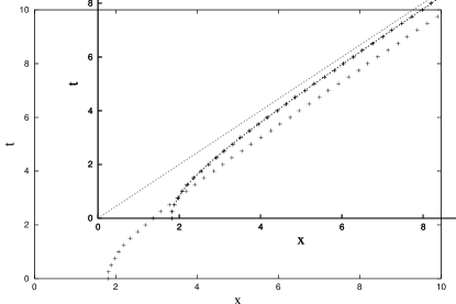
FIG. 3.: Spacetime trajectory for a (1+1)-dimensional bubble started at rest at $t=0$ is well described by the hyperbola $x=\sqrt{R^{2}+t^{2}}$ with $R=1.82$.

We have so far said nothing about induced vacuum decay, in which a bubble may be nucleated with an arbitrary size and shape. As seen in Eq. (15), the spontaneous decay of the vacuum via the bounce costs exactly no energy. However, if the energy of an initial bubble configuration may be accounted for from another source, it need not be zero. We would like to know how such a bubble will evolve given what we know about the bounce. We first consider varying the size of the bubble without changing its interface profile.

Generally the fate of an induced bubble–growth or decay–can be determined by considering the energetics of the corresponding initial value problem. In this case, we do not have a solution for all spacetime, but only a spatial profile at some initial time $t=0$. We will assume that the bubble wall is initially at rest, i.e. that its kinetic energy is zero . The total energy is given by

$$E=\int d^{d}x\ {1\over 2}\left(\partial_{t}\phi_{\rm b}\right)^{2}+{1\over 2}\left(\nabla\phi_{\rm b}\right)^{2}+V(\phi_{\rm b}),$$ (17)

where the static part can again be computed in the thin wall limit. It is $E_{\rm static}=\sigma S_{d}-\epsilon V_{d}$, where $S_{d}$ and $V_{d}$ are the surface and volume of the bubble in $d=D-1$ spatial dimensions. The energy has a local maximum at $R_{E}=(d-1)\sigma/\epsilon$ (recall that the bounce has an action extremum at $R_{B}=d\sigma/\epsilon$). For the interface to move while globally conserving energy it is necessary that it can lower its static energy, so that the difference is converted into kinetic energy. Bubbles with $R>R_{E}$ do so by growing while those with $R<R_{E}$ must shrink. Hence $R_{E}$ defines the critical radius for growth. A particular case is that of the bounce which corresponds to the choice of $R_{B}$ which enforces $E_{\rm static}=0$. The bounce always falls in the class $R>R_{E}$ and therefore always grows. However, it is not the case, as is frequently assumed in the literature, that the bounce radius is the critical radius as defined by the onset of dynamical growth. We plot an example of the energy in 3 spatial dimensions in Fig. 4(a).

(a) $d=3$

(b) $d=1$

FIG. 4.: The dependence of energy and action on the radial coordinate in the thin wall approximation: (a) a “spherical” bubble in 3d. The critical radius for growth $R_{E}$ is the maximum of the energy and is smaller by a factor of $(d-1)/d$ than the radius $R_{B}$ which maximizes that action and corresponds to the zero of energy. (b) In 1d, the critical radius $R_{E}$ goes to zero.

The case of (1+1)-dimensions ($d=1$ above) is special because the interface energy saturates: once the bubble is larger than twice the thickness of the wall, the “surface” term no longer depends on the size of the bubble. Since the bubble can gain kinetic energy by converting false vacuum, a thin wall bubble will always grow in (1+1)-dimensions, i.e. $R_{E}=0$. This is seen clearly in Fig. 4(b), where the thin wall approximation is again assumed. If $\mu$ is a measure of the inverse thickness of the bubble, then the thin wall approximation amounts to $\mu R\gg 1$. In practice, the finite size of the wall profile constrains $\mu$ so that $R_{c}\simeq 1/\mu$ gives a lower limit on the critical bubble size.

We verified this behavior numerically as well as the fact that the thin wall prediction of $R_{E}^{d=2}=R_{B}^{d=1}=1.817$ is an excellent approximation to the real critical value for bubble growth in $d=2$, which occurs between $R=1.810-1.815$. Changing the radius amounts to using $\phi(\rho-R)$ with the analytic form (13) and variable $R$ as an initial condition. We show the trajectories obtained for bubbles with different initial sizes in Fig. 5. Note that the trajectories for bubbles with radii smaller or larger than the bounce asymptote to shifted light cones. Naively, one might have expected all solutions to approach the light cone from the origin.

FIG. 5.: Spacetime trajectories for the motion of several (1+1)-dimensional interfaces started at rest at $t=0$ and with different bubble radii. All trajectories are well described by hyperbolae $x=\pm(x_{0}+\sqrt{R^{2}+t^{2}}$), with origins set at $t=0$. Thus the interface velocity at large times approaches the speed of light as in the case of the bounce, where $x_{0}=0$.

In order to explain these trajectories, we explicitly construct a piecewise solution for all (real) time with an arbitrarily initial size. The real time equations of motion are invariant under a coordinate shift $x\rightarrow x+x_{0}$. Consider cutting the function $\phi_{b}(x,t)$ along $x=0$ at $t=0$ and shifting the positive $x$ piece by a positive amount $x_{0}$ and the negative $x$ piece by $-x_{0}$. In the gap created in the center, extend the value of $\phi(x=0)$ to be constant. This function looks exactly like the bounce at the interfaces but has more true vacuum sandwiched in the middle, see Fig. 6. The boundary conditions on the bounce (4) ensure continuity up to and including first derivates at $\pm x_{0}$. (Excising a homogeneous region in the center, one can similarly generate a smaller bubble.)

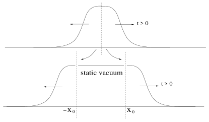
FIG. 6.: Schematic construction at $t=0$ of a solution to the real time equations of motion for all $t>0$.

A constant field in true vacuum is a static solution of the equations of motion, hence the piecewise solution will be static in the region $|x|<x_{0}$ and expand like the bounce outside this region. Moreover, we recall that although $R$ is determined variationally in the thin wall approximation–this freedom is exploited by our initial condition–solving the bounce equation directly (under the assumption of $O(D)$ symmetry) determines $R$ uniquely. The coordinate shift transforms

$$\phi(\sqrt{x^{2}-t^{2}}-R)\rightarrow\phi(\sqrt{(x\mp x_{0})^{2}-t^{2}}-R)\ ,$$ (18)

so the trajectory of the interface is given by $x=\pm(x_{0}+\sqrt{R^{2}+t^{2}})$ in real time, implying that bubbles induced with different sizes will asymptote to different light cones as in Fig. 5.

So far we have altered the bubble size but not its profile. Since to distort the shape would be to perform a variation in function space, it is much more difficult to quantify the difference in the evolution of an arbitrary bubble from that of the bounce. Heuristically, we understand that if a bubble starts out with the wrong profile, it will try to change its shape to the bounce before it expands as described above. The critical size argument can be affected by this: since a small bubble shrinks as it deforms, a slightly supercritical bubble with the wrong shape may still collapse away. A large initial bubble on the other hand will convert the false vacuum energy into kinetic modes which both expand and distort the bubble. We have observed both types of behavior in numerical evolutions.

III Quantum bubbles

Extending the analysis of the previous section to quantum fields introduces a host of new challenges. From the point of view of dynamical equations of motion, we must now consider operator equations, which in fact translate into an infinite Dyson-Schwinger hierarchy of equations for the $n$-point Green’s functions of the theory. For practical purposes, the hierarchy must be truncated somehow, and this truncation introduces an approximation, often in the form of a self-consistent ansatz [19]. Furthermore, even upon keeping a finite number of connected correlation functions the resulting system of coupled equations still describes an infinite number of degrees of freedom with non-linear interactions. Such a system must in general be solved numerically in a finite computer, which can lead to artifactual effects. Thus it is of utmost importance to identify practical approximation schemes that capture the qualitative essence of the dynamical evolution of a quantum field theory as compared with its classical counterpart. This challenge is not devoid of uncertainty since not much is known about the evolution of truly quantum many body systems far away from thermal equilibrium.

The formulation of the problem can be cast into one formalism which has been developed and explored in several works and has resurfaced in recent years with renewed vigor [11, 12, 14]. It is based on a two-particle irreducible (2PI) effective action for the field and the two-point function $\Gamma[\phi,G]$ formalized by Cornwall, Jackiw and Tomboulis (CJT) [11]. The Schwinger-Keldysh closed time path (CTP) is employed to make causality explicit through an appropriate real time prescription in the path integral time contour and associated Green’s functions; hence it is frequently referred to as the CJT or the 2PI-CTP formalism. It is in the evaluation of $\Gamma[\phi,G]$ that some sort of expansion (in loops or in powers of the coupling constant or in powers of $1/N$ for example) is carried out.

In this paper we shall employ the 2PI-CTP formalism at the level of the Hartree approximation, a mean-field approximation which amounts to keeping the 2PI diagrams which are lowest order in coupling constants (bubble diagrams). The Hartree approximation is well understood to be equivalent to a Gaussian variational ansatz in the Schrödinger functional formalism [20] and results in Hamiltonian dynamics [21]. It is also qualitatively similar to the systematic large-$N$ approximation at leading order in $1/N$. For our purposes, $N=1$ and the Hartree approximation is motivated chiefly because it is extremely simplifying. A large $N$ scalar theory is also inappropriate for the description of first order transition dynamics as it results invariably in second order critical phenomena (unless the $O(N)$ symmetry is explicitly broken, whence criticality is erased and the transition becomes an analytical crossover).

Time evolution of spatially inhomogeneous quantum fields, even at this level of approximation has only recently been produced numerically [22, 23, 24]. To our knowledge, the growth of a critical self-consistent quantum field bubble has not been previously demonstrated.

The starting point for the 2PI-CTP formalism is the effective action $\Gamma[\phi,G]$ of [11]:

$$\Gamma[\phi,G]= S[\phi]+\frac{1}{2}i\hbox{Tr}\ln G^{-1}+\frac{1}{2}i\hbox{Tr}D^{-1}(\phi)G$$ (20)

$$+\Gamma_{2}(\phi,G)+\hbox{const.}\ ,$$

where $iD^{-1}(\phi)$ is the classical inverse propagator

$$iD^{-1}(x,y;\phi)=\frac{\delta S[\phi]}{\delta\phi(x)\delta\phi(y)}$$ (21)

and $\Gamma_{2}$ sums the 2PI vacuum to vacuum diagrams with propagators set to $G$ and interaction vertices obtained from the shifted Lagrangian ${\cal L}[\phi\rightarrow\phi+\varphi]$.

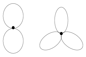
FIG. 7.: Vacuum bubble diagrams in the Hartree approximation for the 2PI effective action of our model. Lines denote the full propagator $G$ in the nontrivial $\phi$ background.

In the Hartree approximation, we consider 2PI diagrams in Fig. 7, hence

$$\Gamma_{2} = -3(\lambda+15g\phi^{2})\int{d^{2}x}\,G(x,x)^{2}$$ (23)

$$\qquad\qquad\qquad-15g\int{d^{2}x}\,G(x,x)^{3}\ .$$

We observe that the two-point function enters into the Hartree approximation only as a local function evaluated at one spacetime point. This is apparent from the diagrams in Fig. 7 which, upon opening a line, become proper self-energy diagrams. The inclusion of any diagram with two or more vertices would introduce non-local kernels in the equations of motion.

The stationarity conditions on the effective action in the absence of sources,

$$\frac{\delta\Gamma[\phi,G]}{\delta\phi}=\frac{\delta\Gamma[\phi,G]}{\delta G}=0,$$ (24)

lead to equations of motion for the field

$$\Bigl{(}\Box+m^{2}+4\lambda\phi^{2}+6g\phi^{4}+12(\lambda+5g\phi^{2})G(x,x)$$ (25)

$$\qquad\qquad\qquad+90g\int{d^{2}x}\,G(x,x)^{2}\Bigr{)}\phi=0\ ,$$ (26)

and for the Wightman two-point function

$$\Bigl{(}\Box+m^{2}+12\lambda\phi^{2}+30g\phi^{4}+12(\lambda+15g\phi^{2})G(x,x)$$ (27)

$$\qquad\qquad\qquad\qquad\qquad+90gG(x,x)^{2}\Bigr{)}G(x,x^{\prime})=0\ .$$ (28)

Let us remark that there are logarithmic and quadratic divergences in the bare theory in the self-energy and energy-momentum tensor respectively. However, any scalar field theory in (1+1)-dimensions is renormalizable using the standard counterterm procedure. For the $\phi^{6}$ interaction, this has been carried out explicitly in an early analysis of the quantum effective potential [25]: the logarithmic divergence from the scalar loop in (1+1)-dimensions affects both the mass and the quartic coupling constant $\lambda$, which need to be renormalized. In practice, even though we solve the equations of motion numerically on a discretized spatial lattice, we introduce time-independent counterterm subtractions as renormalization conditions for the “physical” mass, quartic coupling and energy density in vacuum. We fix the physical (dressed) mass to coincide with the bare mass of the classical theory, i.e. we employ a subtraction (detailed below) which sets the two-point function to zero in the false vacuum. The quadratic divergence in the energy density is just the usual zero-point energy of vacuum, and again we choose to set the energy density in the false vacuum to zero.

In order to solve the system of equations, we need to specify initial data for the field and the two-point function. This is more or less straightforward for the field expectation value, which we identify with the classical field bubble profiles of Section II. Thus, as an ansatz, we initialize the quantum field expectation to have the same shape as the bounce function described in Eq. (13). The initial specification of the two-point function, however, is informed by the full details of the nonequilibrium ensemble. As a starting point, we use the most naive initial conditions possible, which is to ignore the formation of the initial bubble completely. In other words, the two point function is initialized for a zero- or finite-temperature distribution about the false vacuum everywhere in space, including inside the bubble. We are in the process of improving this prescription and comment on this below.

We proceed by decomposing the equal-spacetime propagator in a mode basis. From here on we use $x$ to denote the space coordinate alone instead of spacetime, i.e. $x^{\mu}=(x,t)$ and $G(x^{\mu},x^{\mu})$ can be written as

$$G(x,t)=\sum_{k}|\psi_{k}(x,t)|^{2}(2n_{B}(k)+1)\ ,$$ (29)

where $n_{B}(k)$ is the Bose-Einstein distribution

$$n_{B}=\frac{1}{1-e^{\beta\omega_{k}}}\ .$$ (30)

The mode functions $\psi_{k}$ are initialized in a plane wave basis with the mass of excitations around the false vacuum:

$$\psi_{k}(x)=\frac{e^{ik\cdot x}}{\sqrt{2\omega_{k}}}\ ,$$ (31)

with

$$\omega_{k}=\sqrt{k^{2}+m^{2}}\ .$$ (32)

The mass in the dispersion relation is self-consistently dependent on the values of the mean field and fluctuations. The log-divergent, zero-temperature part of $G$ is renormalized by the subtraction of $G(x,t)$ evaluated at $x=t=0$,

$$G_{R}(x,t)=G(x,t)-G(0,0)\ .$$ (33)

This is equivalent to mass and coupling constant renormalization.

Finally we evolve the field and two-point function according the equations (25) and (27) on a discrete one-dimensional lattice. We employ a variety of lattices corresponding to different physical volumes and lattice spacings and use a fourth order symplectic integrator to step in time. The range in the number of lattice points was between 256 and 2048, with typical lattice spacing of 1/64 to 1/128. Diagnostics performed at regular time intervals give a series of cinematic snapshots of the evolution and measure the components of the energy momentum tensor $\left<T_{\mu\nu}\right>$ as well as the separate components of the energy $\left<T_{00}\right>$, i.e. potential, gradient and kinetic energy.

The results for the evolution of the quantum fields are shown in the next section, where they are also compared to the purely classical field bubbles of Section II.

IV Numerical results

In Section II we have already discussed the paramount importance of Lorentz symmetry in constraining many of the properties of bubble wall propagation. These constraints clearly also apply in the quantum theory at zero temperature.

The first clear difference is that the field profile corresponding to the bubble is no longer purely classical. The quantum modes respond to our (initially) classical background and partially screen it. The result is a dressed bubble, an object with a quasi-classical profile around which the vacuum is disturbed. This self-consistent object is Lorentz invariant and once formed propagates adiabatically, i.e. without further particle creation. Several snapshots of the mean field and 2-point function in Fig. 8 illustrate this behavior, from initial formation to late propagation.

The next important effect of quantum fluctuations is essentially static. Looking at Fig. 8 we also note that while the “height” of the dressed bubble (i.e. the true vacuum expectation value (vev) of the field) is initialized at the classical vev, it will not remain at that value during bubble growth. This is nothing remarkable, only a demonstration of the well known fact that the quantum effective potential differs from the classical potential, and their minima do not coincide. It might make more sense to initialize the field with the true vacuum expectation value given by the quantum effective potential at some loop order. However, given the naive initialization of the two-point function that we employ here, the field will still be perturbed away from this minimum inside the bubble when the two-point function changes. The analyticly computated quantum effective potential treats the mean field as spatially homogeneous. Therefore it cannot be expected to describe accurately the dynamics of the bubble. We discuss this problem and its solution in more detail below and in Section V.

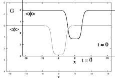
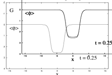
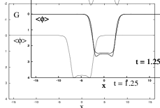
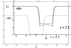
FIG. 8.: Snapshots of the expectation value for classical and quantum field (lower curves) and two-point function $G$ (upper curve) at increasing time intervals. The initial configuration shown in the top left is almost identical in both cases. The evolution shows the quantum bubble relaxing into the minimum energy configuration preferred by the quantum effective potential while being screened by quantum fluctuations. In so doing, it leaves behind excitations inside the bubble and accelerates more rapidly. For presentation, $G$ is shown shifted away from its actual value (equal to zero where $\phi=0$.)

FIG. 9.: The quantum Hartree approximation trajectories for initial bubbles of various sizes are shown as pluses. The lines are interpolations of the classical trajectories shown in Fig. 5. The initial acceleration of the quantum bubble wall is manifestly more rapid, and it approaches its lightcone asymptote more quickly.

At zero temperature, we observe both super- and sub-critical bubbles in the quantum case which grow and decay respectively as in the classical case. We track the position of the bubble wall in time. Despite the fact that the quantum evolution introduces fluctuations absent in the classical case, we see a bubble wall trajectory which is consistent with the classical picture. We observe approximately hyperbolic trajectories which asymptotically approach the speed of light, as shown in Fig. 9. Fig. 8 shows some of the quantitative differences between the classical and the quantum evolution, including the effect of the “roll” down to the minimum of the quantum effective potential. As the field vev changes inside the bubble, it releases potential energy beyond what would happen from the movement of the interface–namely bubble growth–alone. Since this energy is converted into kinetic and gradient energy of the field and fluctuations, this roll can be held responsible for a more rapid acceleration at the initial stage of growth. The energy of the true vacuum in the quantum case is also lower, so the rate of energy release by the bubble growth is larger. Hence, we see the quantum trajectories in Fig. 9 approach their asymptotic value (again unity) more quickly. This is the only significant departure from the particular hyperbolic trajectory predicted by a classical analysis.

We also note that while the classical critical radius for growth was found to be $R_{c}=0.35$, the critical radius in the quantum evolution is around $R_{c}=0.45$. In both cases, the critical radius for growth is a factor of 4 to 5 smaller than the bounce radius $R_{B}$ while relatively close (within a factor of 2) to the lower limit in (1+1)-dimensions for a wall with some thickness $\mu^{-1}$ (i.e. $R_{c}\simeq 1/\mu$). In Section II, we found $\mu^{-1}=0.24$.

It is worth considering whether the accelerated initial growth and the observed change in $R_{c}$ can be understood just from a classical analysis of the bubble using the effective potential instead of the bare potential. Recall that the particular shape of the hyperbolic trajectory is determined in the thin-wall analysis by the shape of the potential through the parameter $R_{B}$. For example, we can compute the effective potential numerically using homogeneous fields and solving a gap equation along the lines of earlier works [26]. From this, we can extract a quasi-classical potential and recalculate $R_{B}$ and $\mu^{-1}$ for this potential. We obtain $R_{B}=0.86$ and $\mu^{-1}=0.25$. We fit the observed value of $R_{B}=1.3$ from the trajectories in Fig. 9. While the classical thin-wall predictions using the quantum effective potential give the correct qualitative changes, they predict the wrong magnitude of the correction. We should also note that parametrically the thin wall approximation ought to be worse in the quantum case since now $\mu R\simeq 3.44$, less than half its classical value.

This rough calculation harkens back to several efforts at applying the bounce analysis to quantum field models with, for example, symmetry breaking due to radiative corrections [27]. The problem in effect stems from the fact that the degrees of freedom which need to be traced over in the calculation of the effective potential cannot be properly integrated out since they participate in the bubble dynamics. We believe that a way out of this dilemma necessitates calculation of a self-consistent bounce, i.e. not only the shape of the mean field but also the full spectrum of interacting fluctuations in its background as prescribed by an effective action. While this is beyond the scope of the present work, we are pursuing it for future publication. Furthermore, with this information in hand, one could hopefully also bring to bear an analysis of the dynamical viscosity experienced by the moving wall at finite temperature, as suggested by other recent results [28, 29].

In the meantime, the observed differences we have described in the shape and trajectory of the purely classical bubble and its dressed quantum counterpart are all that one may expect. At zero temperature, the qualitative characteristics of bubble propagation remain determined by the constraint of Lorentz invariance. Once finite temperature is considered, or alternately in the presence of a Lorentz-violating condensate, bubble propagation can change drastically, and the velocity of domain growth will in general not asymptote to that of light.

Turning now to the last of Coleman’s open questions, we consider the effect of colliding bubbles in the classical and quantum Hartree approximations. Due to the nature of our numerical simulations, we enforce periodic boundary conditions on our one-dimensional lattice at the endpoints. When the bubble interface reaches the end of the lattice, it effectively meets its mirror image or, equivalently, a neighboring bubble wall. Whether the interfaces bounce off of each other or coalesce can then be observed.

We note a surprising result: classically the bubble walls do not coalesce. The collision of the interfaces does temporarily excite wavelengths near the bubble “penetration depth” (the bubble thickness) at low amplitude, but this energy appears to be re-exchanged with the bubble interface. Furthermore, this is a special feature of the bounce profile which is not robust under deformations of the shape of the bubble: other initial bubbles do radiate and decay albeit slowly through collisions, see Fig. 10. We also verified that the stability of the bounce disappears in (2+1)-dimensions where collisions rapidly destroy the spherical symmetry of the bubble.

The (1+1)-dimensional classical bounce solution exhibits truly solitonic behavior in the sense that it is unaltered by scattering off of another (solitonic) bubble. This effect, well known to exist in integrable nonlinear systems [30], is unexpected in our model. In fact, Lohe has considered the linearized perturbations around the static soliton (13) of this model as one example in a parameter family of polynomial potentials (the sine-Gordon model appears as a limiting case); he has shown that there are completely reflected states in one direction from the soliton or bubble wall [31]. This is just a physical consequence of the difference in the mass of elementary excitations about the two vacua: low-lying states in the false vacuum cannot pass through the interface because they have no energy counterpart on the other side. We may take this as suggestive evidence that the two bubble interfaces must repel under these circumstances, although it cannot guarantee the observed almost perfect reflection. If the sign of the $\gamma$-term in the potential (7) is flipped, the initial bubble will collapse and the interfaces will pass through each other, exploiting the $\phi\rightarrow-\phi$ symmetry of the model as they emerge on the other side of the collision region.. We verified this behavior numerically. The classical scattering of our interfaces is thus quite analogous to the scattering of solitons in the sine-Gordon model where both types of behavior (perfect reflection and perfect transmission) obtain even though the vacua are identical [32]. In that case, it is soliton-soliton or soliton-antisoliton solutions which display the two distinct possibilities.

Quantum bubbles by contrast appear to dissipate energy rather efficiently during collisions and especially during the propagation of the interface through the fluctuations created by the collision. Although at the level of our approximation the bubbles still rebound initially from the collision, they quickly lose kinetic energy. By the second or third collision, all semblance of the initial configuration is lost. In order to understand the quantum, or at least semi-classical scattering of the interfaces, one could perform a detailed study along the lines of Ref. [33], adapted for the self-consistent quantum evolution.

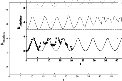
FIG. 10.: Trajectories for bubble interfaces bouncing off of neighboring interfaces. Connected curves show classical trajectories for the bounce (bottom) and distortions thereof (upper curves), while quantum trajectories are shown as data points. The classical bounce and the quantum data are plotted for lattice spacings of 1/64 and 1/128, but the trajectories overlap entirely. The quantum trajectory loses coherence quickly relative even to the distorted classical bubbles.

We present results in Fig. 10, where we plot the classical and quantum trajectories at two different lattice spacings (same physical volume) in order to demonstrate that this effect is not an artifact of the lattice discretization. We also plot classical trajectories of distorted bubbles to show that they decay on a much longer time scale than the quantum bubbles. The trajectories are obtained by following one field value near the true vacuum; in the quantum and classical distorted cases, the apparent loss of periodicity indicates that fluctuations around the true vacuum no longer have a coherent structure. In Fig. 11 we plot a late time snapshot of the field evolution in the classical and quantum cases.

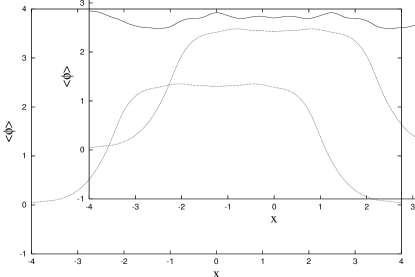
FIG. 11.: Field expectation values for the quantum (upper) and classical (lower) evolution after twelve collisions with neighboring bubbles (effected by means of periodic boundary conditions). The classical bubble still maintains its shape, while the quantum bubble appears to have dissipated its energy into fluctuations around the true vacuum.

V Discussion and conclusions

In this paper we took the first steps towards showing how self-consistent quantum fluctuations can be incorporated in the real time dynamics of bubble interfaces. We have shown that a classical bubble profile becomes dressed by quantum fluctuations, which in turn affect the rate of conversion of the false to true vacuum, i.e. the acceleration of the bubble velocity towards the speed of light. We have also found that the presence of quantum fluctuations promotes substantially more efficient transport of the bubble wall energy into particles at bubble collisions.

There is one inelegant feature of our analysis, namely that the initial conditions for the quantum evolution were informed by the classical bounce calculation in absentia of self-consistent fluctuations. There should exist a solution to the coupled Dyson-Schwinger equations which is analogous to the bounce, the analytic continuation of which amounts to a dressed bubble which expands without radiation (particle creation). Using this configuration as a starting point for an initial value problem would eliminate the unwanted radiation that we observed resulting from the early time response of the vacuum to the nontrivial classical background.

Starting from the 2PI-CTP formalism it is natural to generalize the one-loop computation of the false vacuum decay rate to a self-consistent problem, where fluctuations and the mean-field bubble profile are solved together. The self-consistent nucleation rate and bubble evolution would be accurate to the same level of truncation as the effective action for any approximation, not limited to the Hartree example above. We believe that this intermediate step is necessary before more subtle features of the long time evolution–inevitably entangled with the early time response–can be analyzed quantitatively in detail. We have made progress towards this implementation, which we intend to report in a future work [34].

Knowledge of the spectrum of self-consistent fluctuations will render the inclusion of medium effects such as finite temperature more realistic. It also paves the way for other generalizations of the model and improvements upon the approximation we have employed. A finite temperature analysis in particular may be sensitive to higher loop order interactions which give rise to viscosity effects in linear response around equilibrium. Through analysis of the energy-momentum tensor $\left<T_{\mu\nu}\right>$ we can investigate the emergence of hydrodynamic interface propagation from microscopic physics. We also intend to extend the model to include fermions.

There are many more directions in which a similar analysis may be informative. From numerical solution of a subcritical bubble which decays, we can read the spectrum of asymptotic states. It may be possible that the same states, upon time reversal, would provide the initial conditions necessary to generate a bubble. Such an asymptotic configuration is generically a complicated, correlated many-particle state; however its overlap with a two-body state may hint at the probability of a bubble resonance in a scattering experiment. Stable dynamical solutions such as breathers have long been features of classical field theories. It is unknown whether they are stable upon inclusion of dynamical quantum effects. Finally, there has been a great deal of excitement recently about extended objects such as branes and their dynamics, collisions etc. If there are fields confined to each brane in a homogeneous manner, then the effect of colliding two branes can be cast into a problem very similar to the one explored here with the addition of traces over transverse degrees of freedom.

- [1] R. Becker and W. Döring, Ann. Phys. 24, 719 (1935).
- [2] J. S. Langer, Annals Phys. 41, 108 (1967) [Annals Phys. 281, 941 (1967)].
- [3] S. R. Coleman, Phys. Rev. D 15, 2929 (1977) [Erratum-ibid. D 16, 1248 (1977)]; S. R. Coleman, in C77-07-23.7 HUTP-78/A004 Lecture delivered at 1977 Int. School of Subnuclear Physics, Erice, Italy, Jul 23-Aug 10, 1977.
- [4] See e.g. J. D. Gunton, M. San Miguel and P. S. Sahni, The Dynamics of First Order Phase Transitions, in Phase transitions and Critical Phenomena, Vol. 8, Eds. C. Domb and J.L. Lebowitz (Academic Press, London, 1983).
- [5] For a recent review see e.g. M. Trodden, Rev. Mod. Phys. 71, 1463 (1999) [arXiv:hep-ph/9803479].
- [6] See G. D. Moore and T. Prokopec, Phys. Rev. D 52, 7182 (1995) [arXiv:hep-ph/9506475] for a transport treatment of bubble motion in the standard model at finite temperature and K. Kainulainen, T. Prokopec, M. G. Schmidt and S. Weinstock, [arXiv:hep-ph/0202177] and references therein for a derivation of that transport theory.
- [7] For a hydrodynamic approach to bubble expansion see H. Kurki-Suonio and M. Laine, Phys. Rev. Lett. 77, 3951 (1996) [arXiv:hep-ph/9607382].
- [8] There are many systems in condensed matter where first order transitions are accessible experimentally. The first order transition between the A-B phases of superfluid , presents an example where induced nucleation (presumably by ionizing radiation) is necessary; see P. Schiffer, D. D. Osheroff and A. J. Leggett in Progress in Low Temperature Physics, edited by W.P. Halperin (Elsevier, Amsterdam 1995), Vol. 14; P. Schiffer and D.D. Osheroff, Rev. mod. Phys. 67, 491 (1995) and references therein.
- [9] See V. A. Rubakov and M. E. Shaposhnikov, Usp. Fiz. Nauk 166, 493 (1996) [Phys. Usp. 39, 461 (1996)] [arXiv:hep-ph/9603208], for a review on the possibility of creating sphalerons and other topological field configurations in accelerator experiments.
- [10] J. S. Schwinger, J. Math. Phys. 2, 407 (1961); L. V. Keldysh, Zh. Eksp. Teor. Fiz. 47, 1515 (1964) [Sov. Phys. JETP 20, 1018 (1964)].
- [11] J. M. Cornwall, R. Jackiw and E. Tomboulis, Phys. Rev. D 10, 2428 (1974).
- [12] E. Calzetta and B. L. Hu, Phys. Rev. D 37, 2878 (1988).
- [13] F. Cooper and E. Mottola, Phys. Rev. D 36, 3114 (1987); F. Cooper, S. Habib, Y. Kluger, E. Mottola, J. P. Paz and P. R. Anderson, Phys. Rev. D 50, 2848 (1994) [arXiv:hep-ph/9405352]; D. Boyanovsky, H. J. de Vega, R. Holman, D. S. Lee and A. Singh, Phys. Rev. D 51, 4419 (1995);
- [14] J. Berges, Nucl. Phys. A 699, 847 (2002) [arXiv:hep-ph/0105311]; J. Berges and J. Cox, Phys. Lett. B 517, 369 (2001) [arXiv:hep-ph/0006160].
- [15] G. Aarts, D. Ahrensmeier, R. Baier, J. Berges and J. Serreau, arXiv:hep-ph/0201308.
- [16] A. Ferrera and A. Melfo, Phys. Rev. D 53, 6852 (1996) [arXiv:hep-ph/9512290].
- [17] M. Abney, Phys. Rev. D 55, 582 (1997) [arXiv:hep-ph/9606476]; R. M. Haas, Phys. Rev. D 57, 7422 (1998) [arXiv:hep-ph/9706318]; S. Seunarine and D. W. McKay, Int. J. Mod. Phys. A 16S1A , 354 (2001) [arXiv:hep-th/0011142].
- [18] G. H. Flores, R. O. Ramos and N. F. Svaiter, Int. J. Mod. Phys. A 14, 3715 (1999) [arXiv:hep-th/9903009]; M. Joy and V. C. Kuriakose, arXiv:hep-th/0102177.
- [19] C. D. Roberts and A. G. Williams, Prog. Part. Nucl. Phys. 33, 477 (1994) [arXiv:hep-ph/9403224].
- [20] O. J. Eboli, R. Jackiw and S. Y. Pi, Phys. Rev. D 37, 3557 (1988).
- [21] See e.g. S. Habib, Y. Kluger, E. Mottola and J. P. Paz, Phys. Rev. Lett. 76, 4660 (1996) [arXiv:hep-ph/9509413]; F. Cooper, S. Habib, Y. Kluger and E. Mottola, Phys. Rev. D 55, 6471 (1997) [arXiv:hep-ph/9610345].
- [22] G. Aarts and J. Smit, Phys. Rev. D 61, 025002 (2000) [arXiv:hep-ph/9906538]; M. Salle, J. Smit and J. C. Vink, Phys. Rev. D 64, 025016 (2001) [arXiv:hep-ph/0012346]; M. Salle, J. Smit and J. C. Vink, Nucl. Phys. B 625, 495 (2002) [arXiv:hep-ph/0012362].
- [23] L. M. Bettencourt, K. Pao and J. G. Sanderson, Phys. Rev. D 65, 025015 (2002) [arXiv:hep-ph/0104210]; L. M. Bettencourt, F. Cooper and K. Pao, arXiv:hep-ph/0109108, to appear in Phys. Rev. Lett.
- [24] F. L. Braghin, Phys. Rev. D 64, 125001 (2001) [arXiv:hep-ph/0106338].
- [25] P. K. Townsend, Phys. Rev. D 12, 2269 (1975) [Erratum-ibid. D 16, 533 (1975)].
- [26] L. Dolan and R. Jackiw, Phys. Rev. D 9, 3320 (1974); G. Amelino-Camelia and S. Y. Pi, Phys. Rev. D 47, 2356 (1993) [arXiv:hep-ph/9211211]; N. Petropoulos, J. Phys. G 25, 2225 (1999) [arXiv:hep-ph/9807331]; J. T. Lenaghan and D. H. Rischke, J. Phys. G 26, 431 (2000) [arXiv:nucl-th/9901049].
- [27] E. J. Weinberg, Phys. Rev. D 47, 4614 (1993) [arXiv:hep-ph/9211314]; A. Strumia and N. Tetradis, Nucl. Phys. B 554, 697 (1999) [arXiv:hep-ph/9811438].
- [28] E. A. Calzetta, B. L. Hu and S. A. Ramsey, Phys. Rev. D 61, 125013 (2000) [arXiv:hep-ph/9910334].
- [29] S. Alamoudi, D. G. Barci, D. Boyanovsky, C. A. de Carvalho, E. S. Fraga, S. E. Joras and F. I. Takakura, Phys. Rev. D 60, 125003 (1999) [arXiv:hep-ph/9904390].
- [30] N. J. Zabusky and M. D. Kruskal, Phys. Rev. Lett. 15, 240 (1965); See also K. Lonngren and A. Scott, Solitons In Action. Proceedings Of A Workshop Held At Redstone Arsenal, October 26-27, 1977 Academic Pr.,New York 1978.
- [31] M. A. Lohe, Phys. Rev. D 20, 3120 (1979).
- [32] J. Rubinstein, J. Math. Phys. 11, 258 (1970); For an early review, see A. C. Scott, F. Y. Chu and D. W. McLaughlin, IEEE Proc. 61, 1443 (1973).
- [33] R. Jackiw and G. Woo, Phys. Rev. D 12, 1643 (1975).
- [34] Y. Bergner and L. M. A. Bettencourt, in preparation.