Electromagnetic Polarization Effects due to
Axion Photon Mixing

Pankaj Jain, Sukanta Panda and S. Sarala

Physics Department, I.I.T. Kanpur, India 208016

Abstract: We investigate the effect of axions on the polarization of electromagnetic waves as they propagate through astronomical distances. We analyze the change in the dispersion of the electromagnetic wave due to its mixing with axions. We find that this leads to a shift in polarization and turns out to be the dominant effect for a wide range of frequencies. We analyze whether this effect or the decay of photons into axions can explain the large scale anisotropies which have been observed in the polarizations of quasars and radio galaxies. We also comment on the possibility that the axion-photon mixing can explain the dimming of distant supernovae.

1 Introduction

The mixing of axions with photons and its observable consequences have been analyzed by many authors [1-12]. In the present paper we investigate the changes in the polarization of electromagnetic waves that arise due to its mixing with axions. We are particularly interested in determining if this mixing can explain the polarization anisotropies that have been claimed in Ref. [13, 14, 15].

In Ref. [13, 14] the authors claimed that the observed polarizations from distant radio galaxies and quasars are not isotropically distributed on the dome of the sky. The observable of interest in that study was the angle $\beta=\chi-\psi$, where $\psi$ is the orientation angle of the axis of the radio galaxy and $\chi$ the observed polarization angle after the effect of Faraday rotation is taken out of the data. The authors claimed a dipole anisotropy such that the angle $\beta$ is given by

$$\beta=\vec{\lambda}\cdot\hat{r}$$ (1)

where $\hat{r}$ is a unit vector in the direction of the source. The $\vec{\lambda}$ represent the three parameters of this fit. The magnitude of this vector $|\vec{\lambda}|$ is found to be approximately 0.5 and its direction

$$\hat{\lambda}=[(0\ h,9\ m)\pm(1\ h,0\ m),-1^{o}\pm 15^{o}]\ .$$ (2)

The effect is independent of redshift and was first claimed in Ref. [13] and later verified by a more reliable statistical procedure [17] and by compiling a larger data set [14]. This anisotropy may be a signal of some local effect arising due to the milky way or the local supercluster. However so far it is not known what physical phenomenon could lead to the observed rotation in polarizations. Within the standard model of elementary particles it is difficult to conceive of a physical mechanism which can lead to this effect. The axion field which arises in many extensions of the standard model of particle physics may provide one possible explanation. However so far it is not known whether such a field can consistently explain this effect. This is one of the questions that we study in the present paper.

Another interesting polarization effect in the electromagnetic waves from distant quasars has been claimed in Ref. [15, 16]. It was found that optical polarization are aligned on very large scales. A very striking alignment was found in the region, called A1 in [16], delimited in Right Ascension by $11^{\rm h}15^{\rm m}\leq{\rm RA}\leq 14^{\rm h}29^{\rm m}$ and in redshift by $1.0\leq z\leq 2.3$. The polarizations from quasars in any particular spatial region have a tendency to align with one another. The effect was only seen in patches without any evidence of large scale anisotropy. We point out that the center of the A1 region (see Fig. 1 of Ref. [16]) is exactly opposite to the axis, Eq. 2, of the anisotropy found in Ref. [14]. This might indicate a common origin of these two effects.

Finally we also examine the recent claim [18] that dimming of distant supernovae [19, 20] can be explained in terms of axion photon mixing.

2 Axion-Photon Mixing

The interaction lagrangian of the axions with electromagnetic field can be written as [21]

$${\cal L}_{\rm int}={\alpha N\over 12\pi f_{a}}\phi F_{\mu\nu}\tilde{F}^{\mu\nu}$$ (3)

where $\phi$ is the axion field, $F_{\mu\nu}$ is the electromagnetic field tensor, $f_{a}$ is the scale of PQ [22] symmetry breaking and $N$ is the number of light quark flavors. The current limits on $f_{a}$ are given by

$$f_{a}>10^{10}\ {\rm GeV}$$ (4)

The axion mass is related to the coupling $1/f_{a}$ by

$$m_{a}^{2}=N^{2}{f_{\pi}^{2}m_{\pi}^{2}\over f_{a}^{2}}{m_{u}m_{d}\over(m_{u}+m_{d})^{2}}$$ (5)

where $f_{\pi}$ is the pion decay constant, $m_{\pi}$ the pion mass, and $m_{u}$ and $m_{d}$ the masses of up and down quarks respectively. It is also interesting to consider other pseudoscalar particles which arise in certain extensions of standard model, whose mass is not related to $f_{a}$ by Eq. 5. In most of our discussion below we will take the mass of the pseudoscalar as a free parameter and not given by Eq. 5.

Axions can mix with photons from distant galaxies and lead to rotation of polarization. The basic picture is that the photons emitted by the galaxy can decay into axions as they propagate through the background magnetic field. Since only the photons polarized parallel to the transverse component of the background magnetic field ($\vec{B}_{t}$) decay, this effect can lead to a change in polarization of the electromagnetic wave. Another effect that can also contribute is the mixing of photon with an off-shell axion. This process changes the dispersion relation for the photon polarized parallel to $\vec{B}_{t}$ and hence can lead to changes in polarization. Alternatively the distant galaxies may be emitting axions along with photons. These axions can decay in the presence of magnetic fields into photons which are polarized parallel to $\vec{B}_{t}$. We examine all of these possibilities.

The basic equations can be written as [5, 6],

$$(\omega^{2}+\partial_{z}^{2}-\omega_{p}^{2})A_{\parallel}+gB_{t}\omega\phi=0$$ (6)

$$(\omega^{2}+\partial_{z}^{2}-m_{a}^{2})\phi+gB_{t}\omega A_{\parallel}=0$$ (7)

where $\omega_{p}$ is the plasma frequency, $A_{\parallel}$ is the component of the vector potential parallel $\vec{B}_{t}$, $B_{t}=|\vec{B}_{t}|$ and the coupling $g={\alpha N\over 3\pi f_{a}}$. By making the ansatz,

$$A^{\prime}_{\parallel}=\exp\left(i\omega z-i\int_{0}^{z}{\omega_{p}^{2}(z^{\prime})\over 2\omega}dz^{\prime}\right)A_{\parallel}$$ (8)

$$\phi^{\prime}=\exp\left(i\omega z-i{m_{a}^{2}z\over 2\omega}\right)\phi$$ (9)

and assuming that the frequency $\omega$ is much larger than the mass eigenvalues, the wave equations can be written as,

$$-i\partial_{z}A^{\prime}_{\parallel}+{gB_{t}\over 2}\exp(-i\xi(z)/2\omega)\phi^{\prime}=0$$ (10)

$$-i\partial_{z}\phi^{\prime}+{gB_{t}\over 2}\exp(i\xi(z)/2\omega)A^{\prime}_{\parallel}=0$$ (11)

where

$$\xi(z)=\int_{0}^{z}dz^{\prime}(\omega_{p}^{2}(z^{\prime})-m_{a}^{2})$$ (12)

In arriving at equations 10 and 11 we have ignored second derivatives of $A^{\prime}_{\parallel}$ and $\phi^{\prime}$ since these are slowly varying fields.

We first replace the $\omega_{p}^{2}(z)$ with its mean value ${\overline{\omega}}_{p}^{2}$. In this case, as shown in Ref. [6], the probability for producing the pseudoscalar particles $|\phi(L)|^{2}$ at distance $L$, assuming that $\phi(0)=0$ is equal to

$$P_{\gamma\rightarrow\phi}=|\phi(L)|^{2}=|\phi^{\prime}(L)|^{2}\approx(gB_{t}l)^{2}\sin^{2}\left[{L\over 2l}\right]$$ (13)

where

$$l={2\omega\over\overline{\omega}_{p}^{2}-m_{a}^{2}}\ .$$ (14)

This gives a very small value assuming the current limit for the value of $g$ and the galactic values for $B_{t}$ and $\overline{\omega}_{p}$, independent of the choice of $m_{a}$. The special case where $\overline{\omega}_{p}^{2}$ is accidently equal to $m_{a}^{2}$ is not considered in this paper. The effect is, however, much larger if the variations in the plasma frequency and/or background magnetic field are taken into account [6]. The authors in Ref. [6] assume a Kolmogorov power spectrum, $P_{3N}=C_{N}^{2}k^{-11/3}$ for the electron density fluctuations, where $C_{N}\approx 3\times 10^{-4}$ m^-20/3 for the interstellar medium. The authors then show that for the electromagnetic wave propagating through interstellar medium the probability to produce axions, $P_{\gamma\rightarrow\phi}$, is given by,

$$P_{\gamma\rightarrow\phi} \approx 2.7\times 10^{-5}\left[{g\over 10^{-10}\ {\rm GeV}^{-1}}\right]^{2}\left({\overline{B}_{t}\over\mu{\rm G}}\right)^{2}\left({0.03{\rm cm}^{-3}\over\overline{n}_{e}}\right)^{11/3}$$ (15)

$$\times \left({C_{N}^{2}\over 3\times 10^{-4}\ {\rm m^{-20/3}}}\right)\left({L\over{\rm kpc}}\right)\left({\nu\over 10^{6}\ {\rm GHz}}\right)^{5/3}\left|1-{m_{a}\over\overline{\omega}^{2}_{p}}\right|^{-11/3}$$

In obtaining this result the magnetic field has been assumed to be constant. We have also assumed that the vector potential is approximately constant and kept only the leading order term in the expansion in powers of the fluctuations. Hence this result is valid only if the conversion probability is small. The conversion probability given by this equation is much larger than that implied by Eq. 13. For propagation over galactic distances this probability is still very small compared to unity unless the frequency of the electromagnetic wave is much larger than the optical frequencies. However for supercluster magnetic fields the probability may be equal to unity even at optical frequencies. For example, in the Virgo supercluster of galaxies the magnetic field strength is found to be about 1 $\mu G$ over a very large length scale of 10 Mpc with plasma density of the order of $10^{-6}$ cm^-3 [23]. In order to compute the correlation coefficient $C_{N}$ for the supercluster plasma density we assume, by dimensional analysis, that it scales as $n_{e}^{20/9}$, since $n_{e}$ is the only dimensionful parameter known. This gives $C_{N}^{2}\approx 3.4\times 10^{-14}\ {\rm m}^{-20/3}$. This estimate of $C_{N}$ is not reliable and must be improved in future by direct observations. Using this rough estimate the probability is found to be approximately $8\times 10^{5}$ for $g=10^{-10}$ GeV^-1. This is large enough that it can also significantly affect the CMBR in the direction of the Virgo supercluster. By demanding that $P_{\gamma\rightarrow\phi}<10^{-5}$ for the microwave photons $\nu=50$ GHz we find that $g<0.9\times 10^{-11}$ GeV^-1. This constraint is comparable to the constraint on coupling $g$ obtained from red giants and SN1987A [7, 8, 9] but depends on our assumed extrapolation of $C_{N}$ and hence is not entirely reliable. The constraint imposed by CMBR also implies that

$$P_{\gamma\rightarrow\phi}<6.5\times 10^{3}\left({\nu\over 10^{6}\ {\rm GHz}}\right)^{5/3}$$ (16)

The conversion probability is ofcourse always less than one. The large conversion probability is obtained by using Eq. 15 in the regime where it is not valid. As mentioned above, Eq. 15 is applicable only when the conversion probability is small. In the present case the result, Eq. 16, has to interpreted in the sense that for a considerable range of parameters $P_{\gamma\rightarrow\phi}$ is of order unity for $\nu\geq 10^{6}$ GHz.

We next investigate how the polarization of photons will change due to change in the dispersion of photon because of their mixing with axions. We integrate Eq. 11 by parts, taking $B_{t}$ as constant, to obtain

$$\phi^{\prime}(z)-\phi^{\prime}(0)=-{gB_{t}\over 2}l\left[e^{iz/l}A^{\prime}_{\parallel}(z)-A^{\prime}_{\parallel}(0)-\int_{0}^{z}dz^{\prime}\partial_{z}A^{\prime}_{\parallel}\exp(iz^{\prime}/l)\right]\ .$$ (17)

It is clear that the third term inside the brackets is higher order in $g$ and can be dropped. Substituting this expression for $\phi^{\prime}$ into Eq. 10 we find that

$$\partial_{z}A^{\prime}_{\parallel}(z)=-i{gB\over 2}\phi^{\prime}(0)\exp(-iz/l)+i{g^{2}B_{t}^{2}\over 4}l\left[A^{\prime}_{\parallel}(z)-\exp(-iz/l)A^{\prime}_{\parallel}(0)\right]\ .$$ (18)

The solution to this equation can be written as,

$$A^{\prime}_{\parallel}(L) = A^{\prime}_{\parallel}(0)\exp(i\Gamma(L))-\left({l\over 1+l\Gamma(L)/L}\right)\left[{gB_{t}\over 2}\right]\left(\phi^{\prime}(0)+{gB_{t}\over 2}lA^{\prime}_{\parallel}(0)\right)$$ (19)

$$\times \left[2\sin^{2}\left({L\over 2l}+{\Gamma(L)\over 2}\right)+i\sin\left({L\over l}+\Gamma(L)\right)\right]\exp(i\Gamma(L))$$

where,

$$\Gamma(L)=\left({gB_{t}\over 2}\right)^{2}lL$$ (20)

For large $L$, of the order of galactic or super-galactic scales, the dominant contribution comes from the first term on the right hand side of Eq. 19. This term leads to an additional phase $\Gamma$ for the parallel component of the vector potential in comparison to the perpendicular component. The total photon flux fluctuates due to its conversion into axions.

In the optical frequencies, assuming the galactic values of the magnetic field $B_{t}\approx 1\mu G$ and the plasma density $\overline{n}_{e}\approx 0.03$ cm^-3, we find that $\Gamma(L)$ is of order of $10^{-5}$ for $L\approx 1$ kpc and $g\approx 10^{-10}$ GeV^-1 which is comparable to the probability of conversion of photon into an axion as given by Eq. 15. However for smaller frequencies this gives a much larger result in comparison to Eq. 15. If we assume the Virgo supercluster values of the magnetic field $B_{t}\approx 1\mu G$ and plasma density $\overline{n}_{e}\approx 10^{-6}$ cm^-3 [23] we find that for $m_{a}<<\overline{\omega}_{p}$,

$$l\approx{\nu\over 10^{6}\ {\rm GHz}}\ 0.04\ {\rm Mpc}$$ (21)

and the phase $\Gamma$ can be written as

$$\Gamma(L) = 2.4\times 10^{3}\ \left[{g\over 10^{-10}\ {\rm GeV^{-1}}}\right]^{2}\left({\overline{B}_{t}\over\mu{\rm G}}\right)^{2}\left({10^{-6}{\rm cm}^{-3}\over\overline{n}_{e}}\right)$$ (22)

$$\times \left({L\over 10\ {\rm Mpc}}\right)\left[{\nu\over 10^{6}\ {\rm GHz}}\right]\ .$$

This phase can produce observable changes in the polarization of the electromagnetic wave as we discuss later.

We next compute the contribution to the phase that arises due to fluctuations in the plasma density. We assume, for simplicity, that the background magnetic field is constant. Then solving for $\phi^{\prime}$ in Eq. 11 and substituting into Eq. 10 we find,

$$\partial_{z}A_{\parallel}^{\prime}=-\left({gB_{t}\over 2}\right)^{2}\exp\left(-i{\xi\over 2\omega}\right)\int_{0}^{z}dz^{\prime}\exp\left(i{\xi\over 2\omega}\right)A_{\parallel}^{\prime}$$ (23)

Here we have set $\phi^{\prime}(0)=0$. If $\phi^{\prime}(0)\neq 0$ then we will find another term on the right hand side which can be evaluated easily to leading order in the fluctuations. We discuss this case later. We next write $A_{\parallel}^{\prime}=e^{i\Omega}\approx 1+i\Omega$, where $\Omega$ is in general complex. We set $A_{\parallel}^{\prime}(0)=1$ and hence $\Omega(0)=0$. We assume that $\Omega(L)$ is small and keep only the leading order terms. In order to compute the higher order terms we will require the higher order density correlations functions for the turbulent interstellar (or intergalactic) medium. These correlation functions are, however, unknown and hence it is not possible to go beyond the leading order term. In any case even the leading order calculation is very useful since it can reliably provide us with the parameter ranges where the axion photon mixing effect may be significant. We find that $\Omega(L)$ can be written as

$$\Omega(L)=i\left({gB_{t}\over 2}\right)^{2}\int_{0}^{L}dz\exp\left(-i{\xi\over 2\omega}\right)\int_{0}^{z}dz^{\prime}\exp\left(i{\xi\over 2\omega}\right)$$ (24)

We can now expand $\xi/2\omega$ in terms of the fluctuations in the plasma density to get

$${\xi\over 2\omega}={z\over l}+{1\over 2\omega}{\overline{\omega}_{p}^{2}\over n_{e}}\int_{0}^{z}dz^{\prime}\delta n_{e}$$ (25)

where we have used $\omega_{p}^{2}\propto n_{e}$, $\omega_{p}^{2}=\overline{\omega}_{p}^{2}+\delta\omega_{p}^{2}$ and $n_{e}=\overline{n}_{e}+\delta n_{e}$. Substituting this into Eq. 24 and expanding the right hand side to second order in the fluctuations $\delta n_{e}$ we can write the expectation value $<\Omega>=\Omega_{0}+\delta\Omega$ with

$$\delta\Omega(L)=\left({gB_{t}\over 2}\right)^{2}{2il^{2}\over 8\omega^{2}}\left({\overline{\omega}_{p}^{2}\over\overline{n}_{e}}\right)^{2}e^{-iL/l}I_{1}+\left({gB_{t}\over 2}\right)^{2}{il^{2}\over 4\omega^{2}}\left({\overline{\omega}_{p}^{2}\over\overline{n}_{e}}\right)^{2}(I_{2}-I_{3})$$ (26)

where,

$$I_{1} = \left<\int_{0}^{L}dze^{iz/l}\delta n_{e}\int_{0}^{z}dz_{1}\delta n_{e}\right>$$

$$I_{2} = \left<\int_{0}^{L}dze^{-iz/l}\delta n_{e}\int_{0}^{z}dz_{1}e^{iz_{1}/l}\delta n_{e}\right>$$

$$I_{3} = \left<\int_{0}^{L}dze^{-iz/l}\delta n_{e}\int_{0}^{z}dz_{1}\delta n_{e}\right>$$ (27)

and $\Omega_{0}$ is the contribution obtained by keeping only the mean electron density and can be extracted from Eq. 19.

These integrals can be evaluated by expressing them in terms of the Fourier transform of $\delta n_{e}=\int d^{3}{\bf k}\tilde{n}_{e}({\bf k})e^{i{\bf k}\cdot{\bf x}}$ and using the Kolmogorov power spectrum $\left<\tilde{n}_{e}({\bf k})\tilde{n}_{e}^{*}({\bf k^{\prime}})\right>=P_{3N}(k)\delta^{3}({\bf k}-{\bf k^{\prime}})$, where $k=|{\bf k}|$ and

$$P_{3N}(k)={C_{N}^{2}\over(k^{2}+L_{0}^{-2})^{11/6}}\exp\left(-k^{2}l_{0}^{2}/2\right).$$ (28)

Here $C_{N}^{2}$ is the correlation coefficient, $l_{0}$ is the inner scale and $L_{0}$ the outer scale [24]. In our calculation we set $l_{0}=0$. We have explicitly kept the dependence on the outer scale $L_{0}$ since we find that some of the integrals are infrared divergent which are regulated by this scale. We point out that since $\delta n_{e}$ is real $\tilde{n}_{e}^{*}({\bf k})=\tilde{n}_{e}(-{\bf k})$. We find that $\delta\Omega$ is given by

$$\delta\Omega(L) \approx i{6\over 5}\pi^{2}C_{N}^{2}{l^{2}\over 4\omega^{2}}\left({gB_{t}\overline{\omega}^{2}_{p}\over 2n_{e}}\right)^{2}Ll^{5/3}+{6\over 5}\pi C_{N}^{2}{l^{2}\over 4\omega^{2}}\left({gB_{t}\overline{\omega}^{2}_{p}\over 2n_{e}}\right)^{2}$$ (29)

$$\times \int_{-\infty}^{\infty}dk_{z}{1\over\left(k_{z}^{2}+1/L_{0}^{2}\right)^{5/6}}{1\over{1\over l}-k_{z}}\left[L-{\sin(L/l-k_{z}L)\over{1\over l}-k_{z}}\right]$$

In obtaining this result we have kept only the dominant terms which scale like $L$ in the limit of large $L>>l,L>>L_{0}$. The imaginary part $\Omega_{I}$ of $<\Omega>=\Omega_{R}+i\Omega_{I}$, gives the decay rate of the photons with polarization vectors parallel to the transverse component of background magnetic field. It is related to the production rate of axions by $|\phi^{\prime}(L)|^{2}=2\Omega_{I}$. The real part, $\Omega_{R}$, gives an extra phase factor to the parallel component. The integral in the real part of $\delta\Omega$ can be done numerically. We find,

$$\delta\Omega(L)\approx i{6\over 5}\pi^{2}C_{N}^{2}{l^{2}\over 4\omega^{2}}\left({gB_{t}\overline{\omega}^{2}_{p}\over 2n_{e}}\right)^{2}Ll^{5/3}+{6\over 5}\pi C_{N}^{2}{l^{2}\over 4\omega^{2}}\left({gB_{t}\overline{\omega}^{2}_{p}\over 2n_{e}}\right)^{2}4LlL_{0}^{2/3}$$ (30)

It is clear from Eq. 30 that the $\delta\Omega_{R}/\delta\Omega_{I}\sim(L_{0}/l)^{2/3}$, where $\delta\Omega_{R}$ and $\delta\Omega_{I}$ are defined by $\delta\Omega=\delta\Omega_{R}+i\delta\Omega_{I}$. Hence we find that $\delta\Omega_{R}$ is much larger than $\delta\Omega_{I}$ if the frequency is such that $l<<L$, $l<<L_{0}$ and $L_{0}<<L$. We therefore find that for a wide range of frequencies which satisfy these inequalities the phase factor $\Omega_{R}>>\Omega_{I}$ irrespective of whether the plasma density is uniform or has a fluctuating part. In both cases we find that the contribution to $\Omega_{R}\propto\omega$. For the Virgo supercluster, assuming that $C_{N}^{2}$ scales as $\overline{n}_{e}$ and $L_{0}$ scales as $L$ we find that $\delta\Omega_{R}\approx 9\times 10^{5}$ for optical frequencies $\nu=10^{7}$ GHz and $g=10^{-10}$ GeV^-1. Hence at optical frequencies the real part of $\delta\Omega$ is comparable to the imaginary part. However at lower frequencies the real part is much larger.

We next consider the case when the source is emitting axions along with photons. In this case $\phi^{\prime}(0)\neq 0$. The expression for $A_{\parallel}^{\prime}(L)$ can now be written as

$$A_{\parallel}^{\prime}(L) = A_{\parallel}^{\prime}(0)-i{gB_{t}\over 2}\phi^{\prime}(0)\int_{0}^{L}dz\exp\left(-i{\xi\over 2\omega}\right)$$ (31)

$$- \left({gB_{t}\over 2}\right)^{2}A_{\parallel}^{\prime}(0)\int_{0}^{L}dz\exp\left(-i{\xi\over 2\omega}\right)\int_{0}^{z}dz^{\prime}\exp\left(i{\xi\over 2\omega}\right)$$

In order to compute the polarization properties of the electromagnetic wave after propagation through a large distance $L$ we need to compute the correlations $<A_{\parallel}^{\prime*}(L)A_{\parallel}^{\prime}(L)>$ and $<A_{\perp}(L)A_{\parallel}^{\prime*}(L)>$. We ignore all terms which involve third and higher powers of the coupling $g$. Furthermore we include only those terms which scale like $L$ for very large values of $L>>l$. With these requirements it is clear that only three terms contribute to $<A_{\parallel}^{\prime*}(L)A_{\parallel}^{\prime}(L)>$. These are $|A_{\parallel}^{\prime}(0)|^{2}$,

$$\left<\left|i{gB_{t}\over 2}\phi^{\prime}(0)\int_{0}^{L}dz\exp\left(-i{\xi\over 2\omega}\right)\right|^{2}\right>\ ,$$ (32)

and

$$\left<-A_{\parallel}^{\prime*}(0)\left({gB_{t}\over 2}\right)^{2}A_{\parallel}^{\prime}(0)\int_{0}^{L}dz\exp\left(-i{\xi\over 2\omega}\right)\int_{0}^{z}dz^{\prime}\exp\left(i{\xi\over 2\omega}\right)+c.c.\right>\ .$$ (33)

The second term (Eq. 32) given above is equal to the result given in Eq. 15 upto an overall factor of $|\phi^{\prime}(0)|^{2}$. The third term, given in Eq. 33, is equal to the RHS of Eq. 24 (plus its complex conjugate) up to an overall factor of $iA_{\parallel}^{\prime*}(0)A_{\parallel}^{\prime}(0)$. The fluctuating part of this expression is evaluated in Eq. 30. Similarly the only nontrivial term that contributes to $<A_{\perp}(L)A_{\parallel}^{\prime*}(L)>$ involves the expectation value of the third term on the RHS of Eq. 31 which is already evaluated in Eq. 30. We point out that the expectation value of the second term on the RHS of Eq. 31 does not scale like $L$ in the limit of large $L$. Hence the terms which involve interference of this term with a term independent of fluctuations is neglected. We, therefore, find that the only change introduced due to $\phi^{\prime}(0)\neq 0$ is an extra term in $<A_{\parallel}^{\prime*}(L)A_{\parallel}^{\prime}(L)>$ which arises due to decay of axions. This is the term given in Eq. 32 and upto an overall factor of $|\phi^{\prime}(0)|^{2}$, its expression is given in Eq. 15.

We next compute the changes in polarization induced by the phase $\Omega_{R}$ due to axion photon mixing. We neglect the imaginary part of $\Omega$ in the following discussion. As shown above it is in general much smaller than the real part. Furthermore its effect can be easily included by multiplying the component of vector potential (or the electric field) parallel to $\vec{B}_{t}$ by $e^{-\Omega_{I}}$. If the incident electromagnetic wave is unpolarized then the phase $\Omega_{R}$ does not produce any additional effect. However if the incident beam is already polarized then $\Omega_{R}$ can change also its polarization. Let’s consider the simple case of a monochromatic wave,

$$E_{x} = a_{1}\exp(i\alpha_{1}-i\omega t)$$

$$E_{y} = a_{2}\exp(i\alpha_{2}-i\omega t)$$ (34)

where $E_{x}$ and $E_{y}$ are the two transverse components of the electromagnetic wave. By choosing the coordinate axis such that the y-axis is aligned along the direction of the transverse component of the background magnetic field, we find that after propagation through the medium the y component of the electric field $E_{y}$ acquires an additional phase $\Omega_{R}$. Hence the final values of the Stokes parameters are given by

$$S_{0} = a_{1}^{2}+a_{2}^{2}$$ (35)

$$S_{1} = a_{1}^{2}-a_{2}^{2}$$ (36)

$$S_{2} = 2a_{1}a_{2}\cos(\Delta+\Omega_{R})$$ (37)

$$S_{3} = 2a_{1}a_{2}\sin(\Delta+\Omega_{R})$$ (38)

where $\Delta=\alpha_{2}-\alpha_{1}$. The linear polarization angle $\psi$ is then given by

$$\tan 2\psi={S_{2}\over S_{1}}={2a_{1}a_{2}\cos(\Delta+\Omega_{R})\over a_{1}^{2}-a_{2}^{2}}$$ (39)

The degree of polarization $P=(S_{1}^{2}+S_{2}^{2}+S_{3}^{2})^{1/2}/S_{0}$ remains equal to unity. Similarly the degree of circular polarization defined as $P_{C}=|S_{3}|/S_{0}$ is given by

$$P_{C}=\left|2a_{1}a_{2}\sin(\Delta+\Omega_{R})\right|/(a_{1}^{2}+a_{2}^{2})$$ (40)

and the degree of linear polarization $P_{L}=(S_{1}^{2}+S_{2}^{2})^{1/2}/S_{0}$ is given by

$$P_{L}=[(a_{1}^{2}-a_{2}^{2})^{2}+4a_{1}^{2}a_{2}^{2}\cos^{2}(\Delta+\Omega_{R})]^{1/2}/S_{0}\ .$$ (41)

We see that the linear polarization angle $\psi$, the degree of circular polarization $P_{C}$ and the degree of linear polarization $P_{L}$ all depend in a precise manner on the frequency $\omega$ of the incident wave. If we assume that $\Omega_{R}$ is small then these depend linearly on $\omega$. In general these are oscillatory functions of $\omega$. On the other hand the degree of polarization $P$ is independent of frequency. Hence we can easily check this effect by analyzing spectral data from distant AGNs at optical and higher frequencies.

If the incident beam is quasi-monochromatic the above analysis goes through with minimal modification. The wave now need not be completely polarized. We may write its coherency matrix as

$${\bf J}=\left(\matrix{J_{11}&J_{12}\cr J_{21}&J_{22}}\right)$$ (42)

where $J_{ij}=<E^{*}_{i}(t)E_{j}(t)>$ and $J_{21}=J_{12}^{*}$ [25]. After propagating through the magnetic field which is assumed to be pointing in the $\hat{y}$ direction we find that the y-component $E_{2}$ of the electric field acquires an additional phase $\Omega_{R}$. Hence the coherency matrix changes to

$${\bf J}=\left(\matrix{J_{11}&e^{i\Omega_{R}}J_{12}\cr e^{-i\Omega_{R}}J_{21}&J_{22}}\right)$$ (43)

The Stokes parameters can be written as $S_{0}=J_{11}+J_{22}$, $S_{1}=J_{11}-J_{22}$, $S_{2}=e^{i\Omega_{R}}J_{12}+c.c.$ and $S_{3}=i(e^{-i\Omega_{R}}J_{21}-c.c.)$. Parametrizing $J_{12}=je^{i\delta}$ we find that $S_{2}=2j\cos(\delta+\Omega_{R})$ and $S_{3}=2j\sin(\delta+\Omega_{R})$. We again find that the degree of polarization is independent of $\Omega$ but the orientation of linear polarization as well as the degree of linear and circular polarization ($P_{L}$ and $P_{C}$) become oscillatory functions of $\omega$ due to their dependence on $\Omega_{R}$.

3 Astrophysical Applications

We next examine if the astrophysical effects discussed in the introduction can be explained in terms of axion photon mixing. As we have seen the effect is too small for the interstellar magnetic fields. However the effect can be large and produce observable consequences for the case of Virgo supercluster magnetic fields, especially at optical frequencies. We first consider the polarization alignment effect claimed by Hutsemekers [15]. This effect can be explained by the depletion of the photons polarized parallel to $\vec{B}_{t}$. We point out that the real part of $\Omega$ by itself cannot explain this effect. As explained in the introduction, a very striking alignment was found in the region A1 in ref. [16], which is bounded in Right Ascension by $11^{\rm h}15^{\rm m}\leq{\rm RA}\leq 14^{\rm h}29^{\rm m}$ and in redshift by $1.0\leq z\leq 2.3$. In Ref. [16] it is also shown that the quasar polarization in the region A1 show alignment with the supergalactic plane. By invoking coherent cluster magnetic field it may be possible to explain the existence of large scale correlation. The region A1 turns out to be in the direction of the Virgo supercluster and this appears to be a promising explanation. As pointed out in Ref. [16] the correlation with the supergalactic plane may be evidence in favor of a propagation effect such as axion photon mixing. An alternate possibility, also mentioned in Ref. [16], is extinction due to dust. However this explanation suffers from two drawbacks. The first problem is that the effect is redshift dependent, i.e. the regions which show alignment are bounded in redshift as well as in angular coordinates. Secondly one finds that in general the distribution of the degree of polarization for the radio quiet (RQ) along with optically selected non-broad absorption line quasars (O) differs from the distribution of the broad absorption line (BAL) quasars. Precisely the same difference between these different types of quasars is also seen in the A1 region [16]. If the supercluster magnetic field causes the alignment in polarization due to decay of $A_{\parallel}$ then this difference would not be preserved in the A1 region.

It, therefore, seems that a propagation effect is not likely to provide an explanation for this effect. This would, however, imply that the quasar polarizations are intrinsically aligned with one another over cosmologically large distances. Correlations over cosmological distances violate the basic assumption of isotropy and homogeniety of the Universe. Here we propose an alternate mechanism which explains these observations in terms of a propagation effect related to axion photon mixing. We first notice that there are very few RQ+O quasars in the A1 region which satisfy the cut $p>0.6$ % imposed on the data [15]. Hence these quasars do not contribute significantly to the alignment effect. We next assume that the quasars are emitting axions along with the photons. During propagation the axions decay into photons in the presence of background magnetic field. The decay probability of axions is also given by Eq. 15. The emitted photon is polarized in the direction parallel to the transverse magnetic field. The axion photon coupling is assumed to be such that in the optical frequencies the decay probability of axions, or that of photons, from distant quasars is small, less than about 1 %. The total photon flux generated due to decay of axions is equal to the product of the initial axion flux $\Phi$ and its decay probability $P_{\phi\rightarrow\gamma}$. We further assume that for the BAL quasars the initial axion flux $\Phi$ is large enough at optical frequencies such that it leads to significant change in polarization during propagation. In order to explain the Hutsemekers effect we require that the axion flux is of the same order of magnitude as the photon flux from BAL quasars, if the probability $P_{\phi\rightarrow\gamma}\approx 1$ %. In the current paper we will not address the question of emission rate of axions from quasars since the basic physics of the interior of the quasars is not well understood. For the (RQ+O) quasars we assume that the emitted axion flux is small enough such that it does not affect the optical polarizations. The distribution of the degree of polarization for the (RQ+O) quasars will, therefore, be unaffected due to axion photon mixing. However the degree of polarization for the case of BAL quasars will be determined primarily by the propagation effects. Hence this mechanism explains the observed difference between the BAL and (RQ+O) quasars.

The redshift dependence of the Hutsemekers effect [15, 16] is difficult to explain even with the axion decay mechanism discussed above. However we notice that the dominant contribution to the effect comes from the A1 region which can be explained in terms of the Virgo supercluster magnetic fields. The strong alignment of the polarizations with the supercluster plane, as shown in Fig. 3 of Ref. [16], provides further support for this explanation. Some redshift dependence may be obtained due to the evolution of the quasars with redshift. It is possible that the axion emission rate of quasars is redshift dependent and hence only quasars within a certain redshift interval give dominant contribution, with the remaining quasars dominantly contributing noise. It is also possible that the dominant contribution to the effect comes from a few clusters within our astrophysical neighbourhood which can then also contribute to the observed redshift dependence. This can be studied by collecting a larger data sample and putting appropriate cuts on the redshift.

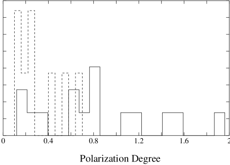
It is interesting to note that the observed difference between the BAL and RQ+O quasars in the direction of the Virgo supercluster allows us to put a very stringent constraint on the pseudoscalar photon coupling $g$ in the limit of $m_{a}<<\overline{\omega}_{p}$ provided we assume our extrapolated value of the correlation coefficient $C_{N}$. We may isolate the influence of the Virgo supercluster by taking only the region in which a large Faraday Rotation Measure is observed. This corresponds to a patch of $20^{o}$ radius around the center of the Virgo supercluster (RA=$12^{\rm h}28^{\rm m}$, DEC=$12^{o}40^{\prime}$) [23]. We find that in this region there are 16 BAL quasars and 9 RQ+O quasars among the objects given in table 2 of Ref. [16]. The difference between these two types of quasars persists in this region also as can be seen in Fig. 1. If the photon to axion conversion probability is large, i.e. $P_{\gamma\rightarrow\phi}>0.1$, then this difference would be completely washed out due to propagation through the Virgo supercluster. This is because the degree of polarization $p$ of RQ+O quasars peaks at very small values ($p\approx 0.2$ %) and we find no quasars in this category with $p>2$ %. This observation implies that the photon decay probability $P_{\gamma\rightarrow\phi}<1$, where the upper limit, unity, is chosen in order to obtain a conservative upper bound on $g$. By using Eq. 15 and the parameters for the Virgo supercluster, given in the discussion following Eq. 15, we find that

$$g<10^{-13}\ {\rm GeV}^{-1}\left[{3.4\times 10^{-14}\ {\rm m}^{-20/3}\over C_{N}^{2}}\right]\left[{1\ \mu{\rm G}\over B_{t}}\right]\left[{\overline{n}_{e}\over 10^{-6}\ {\rm cm}^{-3}}\right]\left[{10\ {\rm Mpc}\over L}\right].$$ (44)

The reliability of this constraint depends on our assumed extrapolation of the correlation coefficient $C_{N}$ for the supercluster. In future it is clearly of interest to obtain this parameter by direct observations which can lead to a more reliable constraint.

Figure 1: The distribution of polarization degree $p$ (in %) for the BAL quasars (solid line) and the RQ+O quasars (dashed line) for a patch of $20^{o}$ radius centered around the Virgo supercluster.

In the radio frequencies ($\sim 1$ GHz) the effect is clearly very small. The dominant contribution is given by $\delta\Omega_{R}$ assuming Virgo supercluster parameters, given in the discussion following Eq. 30. We find that for radio frequencies $\nu=1$ GHz, $\delta\Omega_{R}\approx 0.1$ for $g=10^{-10}$ GeV^-1 with $m_{a}<<\overline{\omega}_{p}$. The appropriate value of $g$ is, however, likely to be much smaller than $g=10^{-10}$ GeV^-1. We next investigate whether the proposed emission of axions due to quasars can explain this effect. Given a large enough flux of axions it is clearly possible to obtain an observable effect on the polarization at radio frequencies. The probability for decay of axions into photons $P_{\phi\rightarrow\gamma}$ in the presence of background magnetic fields is also given by the result given in Eq. 15. Using the CMBR constraint on the coupling $g$ we find that the $P_{\phi\rightarrow\gamma}\leq 6.5\times 10^{-7}$ at radio frequencies $\nu\sim 1$ GHz. Hence in order that axions decay can lead to observable consequences the axion flux has to be roughly $10^{6}$ times larger than the photon flux $F_{\gamma}$ at radio frequencies. The photon flux at radio frequencies is given by $C/\nu^{q}$ where $C$ is a constant and the spectral index $q$ varies roughly between 0.5 to 2 and is in general larger for larger frequencies. Assuming that the axion flux from quasars is indeed $10^{6}$ times larger than the photon flux at radio frequencies and that its spectral dependence is given by $A/\nu^{p}$, where $A$ and $p$ are constants, we find $p\geq q+5/3$ in order that photon spectrum is not in conflict with observations. Assuming that $q\approx 0.8$ at radio frequencies we find that $p\approx 2.5$. The axion luminosity of the quasar is given approximately by $4\pi L^{2}A/[(p-1)\nu_{c}^{p-1}]$, where $\nu_{c}$ is the lower cutoff on the frequency and $L$ is the total distance of propagation. We, therefore, find that the axion luminosity is larger than roughly $10^{6}$ times the radio photon luminosity. For most quasars this is one to two orders of magnitude larger than their total bolometric luminosity. This large luminosity required suggests that this mechanism is disfavored and we do not pursue it further.

Another mechanism that might be relevant for explaining the anisotropy in radio waves involves the presence of background axion field. As shown in Ref. [4] the rotation in the linear polarization angle due to a background magnetic field is equal to $g\Delta\phi/2$ where $\Delta\phi$ is the total change in the background axion field along the trajectory of the electromagnetic wave. If we assume that the axion field in our neighbourhood shows a dipole distribution, $\phi(\vec{r})=\phi_{0}(r)\cos(\Theta)$ where $\Theta$ is the angle with respect to the dipole axis and $\phi_{0}(0)$ is of order $1/g$, then the dipole anisotropy claimed in Ref. [13, 14] can be explained. This explanation requires that the axion field at very large distances, which correspond to the positions of the quasars, is relatively smooth. The random component of the axion field should have a strength smaller than $1/g$. However it is difficult to theoretically justify the existence of such a dipole distribution of the axion field and hence this explanation is also not very compelling.

Finally we examine the recent claim [18] that the observed supernova dimming [19, 20] at large redshifts can be explained in terms of axion photon mixing. It has been pointed out that axion photon mixing is unlikely to provide an explanation because inclusion of the intergalactic plasma density leads to a considerable reduction of the effect [26]. Furthermore it also gives rise to a spectral dependence which is incompatible with observations [26]. The intergalactic parameters used in Ref. [26] are $B=10^{-9}$ Gauss and $\overline{n}_{e}=10^{-7}$ cm^-3. However in Ref. [27] the authors argue that the intergalactic plasma density is likely to be much smaller than this. By using $\overline{n}_{e}=10^{-8}$ cm^-3 it is found that the axion photon mixing can provide an explanation for the dimming effect [27, 28]. Here we examine the magnitude of the effect due to the fluctuating part of the plasma density as given in Eq. 15. Here again if we assume that $L_{c}<<l$ then the $l$, and hence the spectral, dependence goes away. The result in this case can be obtained by calculating $|\phi^{\prime}(L_{c})|^{2}$ which is the probability $P_{\gamma\rightarrow\phi}$ over a single coherence length and then adding all the contributions over the entire propagation distance. The decay probability over a single coherence length is given by [6]

$$P_{\gamma\rightarrow\phi}=\left[{gB_{t}\overline{\omega}_{p}^{2}\over 2\overline{n}_{e}(\overline{\omega}_{p}^{2}-m_{a}^{2})}\right]^{2}<I>$$ (45)

where

$$I=\left|\int_{0}^{L_{c}}dz\delta n_{e}\exp\left(i{\overline{\omega}_{p}^{2}-m_{a}^{2}\over 2\omega}z\right)\right|^{2}\ .$$ (46)

We then find, using $l>>L_{c}$, that

$$<I>=4\pi\int_{-\infty}^{\infty}dk_{z}\int_{0}^{\infty}dk_{T}^{2}{\sin^{2}(k_{z}L_{c}/2)\over k_{z}^{2}}P_{3N}$$ (47)

Here $P_{3N}=C_{N}^{2}/(k_{z}^{2}+k_{T}^{2}+1/L_{c}^{2})^{11/6}$ where the outer length $L_{0}$ has been set equal to the coherence length. We perform the $k_{T}$ integral to find

$$<I>={24\over 5}\pi C_{N}^{2}{L_{c}^{8/3}\over 2^{5/3}}\int_{0}^{\infty}dx{\sin^{2}x\over x^{2}}{1\over(x^{2}+1/4)^{5/6}}$$ (48)

The remaining integral can now be done numerically and is found to be approximately equal to 2. It is clear that the effect is independent of $\nu$. Adding the contributions from the entire propagation distance we need to replace $L_{c}^{8/3}\rightarrow LL_{c}^{5/3}$. Here we have assumed that the total effect is small and the initial axion flux is negligible. We have also ignored the fact that magnetic fields in different domains are aligned in different directions. A more reliable summation over different domains in obtained in Ref. [29]. Here we are only interested in an order of magnitude estimate and hence these additional refinements are unnecessary. In order to estimate the magnitude of the effect we take $L=1$ Gpc, $L_{c}=0.1$ Mpc, $g=10^{-11}$ GeV^-1, $n_{e}=10^{-7}$ cm^-3 and again assume that $C_{N}^{2}$ scales as $n_{e}^{20/9}$. We point out that the parameters $L_{c}$, $g$ and $C_{N}$ are subject to considerable uncertainty. We have chosen a range which is allowed by current observations and for which the effect is significant and independent of $\nu$. With these choice of parameters we find that $P_{\gamma\rightarrow\phi}\approx 1.5$, i.e. the conversion probability is of order unity. It is clear that the range of allowed parameter space is even larger if we use $n_{e}=10^{-8}$ cm^-3. Hence we cannot exclude the possibility that axion photon mixing may be responsible for the dimming of distance supernovae.

4 Conclusions

In conclusion we have analyzed the mixing of axions with photons. We have determined how the dispersion relations of the electromagnetic waves are modified due to the presence of axions. We found that for a wide range of parameters this provides the dominant contribution to the changes in polarization of electromagnetic waves due to mixing with axions. We have also determined whether the existence of axions can explain the large scale anisotropies claimed in References [13, 14, 15]. We find that the Hutsemekers [15] effect may be explained by the supercluster magnetic fields if we assume that quasars emit axions such that their flux is of the order of or larger than the photon flux at optical frequencies. The Birch effect [13, 14] may also be explain by assuming axion emission from radio galaxies and quasars but requires a very large flux at radio frequencies. Its explanation in terms of axions is therefore disfavored. Finally we have estimated the contribution of the fluctuations in the plasma density to the dimming of distant supernovae due to axion photon mixing. We find that this effect can be rather large and for a considerable range of currently allowed parameter space can provide an explanation for the supernova dimming.

Acknowledgements: We thank John Ralston, Ajit Srivastava and Mahendra Verma for very useful comments. This work is supported in part by a grant from Department of Science and Technology, India.

References

- [1] P. Sikivie, Phys. Rev. Lett. 51, 1415 (1983); Phys. Rev. D 32, 2988 (1985).
- [2] L. Maiani, R. Petronzio and E. Zavattini, Phys. Lett. B175, 359 (1986).
- [3] P. Sikivie, Phys. Rev. Lett. 61, 783 (1988).
- [4] D. Harari and P. Sikivie, Phys. Lett. B 289, 67 (1992).
- [5] G. Raffelt and L. Stodolsky, Phys. Rev. D 37, 1237 (1988).
- [6] E. D. Carlson and W. D. Garretson, Phys. Lett. B 336,431 (1994).
- [7] L. J. Rosenberg and K. A. van Bibber, Phys. Rep. 325 1 (2000).
- [8] G. Raffelt, Ann. Rev. Nucl. Part. Sci. 49, 163 (1999), hep-ph/9903472.
- [9] J. W. Brockway, E. D. Carlson and G.G. Raffelt, Phys. Lett. B383, 439 (1996), astro-ph/9605197; J. A. Grifols, E. Masso and R. Toldra, Phys. Rev. Lett. 77, 2372 (1996).
- [10] W.-T. Ni, Phys. Rev. Lett. 38, 301 (1977); M. Sachs, General Relativity and Matter (Reidel, 1982); M. Sachs, Nuovo Cimento 111A, 611 (1997); C. Wolf, Phys. Lett. A132, 151 (1988); ibid A145, 413 (1990); R. B. Mann, J. W. Moffat, and J. H. Palmer, ibid 62, 2765 (1989); R. B. Mann and J. W. Moffat, Can. J. Phys. 59 1730 (1981); D. V. Ahluwalia and T. Goldman, Mod. Phys. Lett. A28, 2623 (1993); C. M. Will, Phys. Rev. Lett. 62, 369 (1989); J. P. Ralston, Phys. Rev. D51, 2018 (1995).
- [11] S. Kar, P. Majumdar, S. Sengupta and A. Sinha, gr-qc/0006097; P. Majumdar and S. Sengupta, Class. Quant. Grav. 16, L89 (1999); P. Das, P. Jain and S. Mukherjee, hep-ph/0011279, Int. Jour. of Mod. Phys. A16, 4011 (2001).
- [12] S. M. Carroll, G. B. Field and R. Jackiw, Phys. Rev. D 41, 1231 (1990).
- [13] P. Birch, Nature, 298, 451 (1982)
- [14] P. Jain and J. P. Ralston, Mod. Phys. Lett. A14, 417 (1999).
- [15] D. Hutsemekers, Astronomy and Astrophysics, 332, 410 (1998).
- [16] D. Hutsemekers and H. Lamy, Astronomy and Astrophysics, 367, 381 (2001).
- [17] D. G. Kendall and A. G. Young, MNRAS, 207, 637 (1984).
- [18] C. Csaki, N. Kaloper, J. Terning, Phys. Rev. Lett. 88, 161302, (2002); hep-ph/0112212.
- [19] S. Perlmutter et al, ApJ 517, 565 (1999).
- [20] A. G. Riess et al, ApJ 116, 1009 (1998); A. G. Riess et al, astro-ph/0104455.
- [21] L. M. Krauss, in the Proceedings of the Yale Theoretical Advanced Study Institute, High Energy Physics (1985), edited by Mark J. Bowick and Feza Gursey.
- [22] R. D. Peccei and H. Quinn, Phys. Rev. Lett. 38, 1440 (1977); Phys. Rev. D16, 1791 (1977).
- [23] J. P. Vallee, The Astronomical Journal 99, 459 (1990).
- [24] J. W. Armstrong, B. J. Rickett and S. R. Spangler, ApJ 443, 209 (1995).
- [25] L. Mandel and E. Wolf, Optical Coherence and Quantum Optics (1995), Cambridge University Press.
- [26] C. Deffayet, D. Harari, J. P. Uzan, M. Zaldarriaga, hep-ph/0112118.
- [27] C. Csaki, N. Kaloper, J. Terning, hep-ph/0112212.
- [28] E. Mörtsell, L. Bergström, A. Goobar, astro-ph/0202153
- [29] Y. Grossman, S. Roy and J. Zupan, hep-ph/0204216.